Heavy Particle Signatures in Cosmological Correlation Functions with Tensor Modes

Abstract

We explore the possibility to make use of cosmological data to look for signatures of unknown heavy particles whose masses are on the order of the Hubble parameter during the time of inflation. To be more specific we take up the quasi-single field inflation model, in which the isocurvaton $\sigma$ is supposed to be the heavy particle. We study correlation functions involving both scalar ($\zeta$) and tensor ($\gamma$) perturbations and search for imprints of the $\sigma$-particle effects. We make use of the technique of the effective field theory for inflation to derive the $\zeta\sigma$ and $\gamma\zeta\sigma$ couplings. With these couplings we compute the effects due to $\sigma$ to the power spectrum $\langle\zeta\zeta\rangle$ and correlations $\langle\gamma^{s}\zeta\zeta\rangle$ and $\langle\gamma^{s_{1}}\gamma^{s_{2}}\zeta\zeta\rangle$, where $s$, $s_{1}$ and $s_{2}$ are the polarization indices of gravitons. Numerical analyses of the $\sigma$-mass effects to these correlations are presented. It is argued that future precise observations of these correlations could make it possible to measure the $\sigma$-mass and the strength of the $\zeta\sigma$ and $\gamma\zeta\sigma$ couplings. As an extension to the $N$-graviton case we also compute the correlations $\langle\gamma^{s_{1}}\cdots\gamma^{s_{N}}\zeta\zeta\rangle$ and $\langle\gamma^{s_{1}}\cdots\cdots\gamma^{s_{2N}}\zeta\zeta\rangle$ and their $\sigma$-mass effects. It is suggested that larger $N$ correlation functions are useful to probe larger $\sigma$-mass .

1 Introduction

It has been by now well accepted that the inflationary expansion in the early Universe is the key to solve various problems in the Big Bang cosmology. The methods to obtain the information during inflation have been developed in various ways. One of the far-sighted theoretical bases has been laid down by Maldacena [1], who applied standard quantum field theories to single-field inflation cosmology and computed the three-point functions involving primordial fluctuations, $\zeta$ (scalar fluctuation) and $\gamma_{ij}$ (tensor fluctuation or ‘graviton’). A special attention was paid to the three-point function of $\zeta$, because it tells us much about the deviation from the Gaussian features of the cosmic state, often referred to as ‘non-Gaussianity’ [2].

Another intriguing and closely related approach was put forward by Cheung et al. [3], who constructed the ‘Effective Field Theory (EFT) of Inflation’ (see also Refs. [4] and [5]). In this theory, the scalar fluctuation $\zeta$ is interpreted as the Nambu-Goldstone mode associated with the spontaneous breaking of the time diffeomorphism invariance. A symmetry argument allows us to consider a more general framework than Maldacena’s by using a technique analogous to the low-energy pion physics.

Although general single field inflationary models have been explored to a considerable extent, there exists another avenue of investigation in inflationary models that contain multiple fields [6, 7, 8, 9]. A class of models is such that, in the space of multi-fields, there is a flat slow-roll direction and all others are isocurvature directions associated with isocurvatons whose masses are on the order of the Hubble parameter $H$. This class of models is called ‘quasi-single field inflation’ and Chen and Wang [10] have pointed out that the massive isocurvaton, which they denoted by $\sigma$, may have important observable effects on cosmological perturbation. The magnitude of the Hubble parameter during inflation may be inferred by the formula

$$H\approx 2.5\times 10^{13}\>\left(\frac{r}{0.01}\right)^{1/2}\quad{\rm GeV}\>,$$ (1.1)

where $r$ is the so-called tensor-to-scalar ratio. If quasi-single field inflation models were realized in Nature and if $r\sim 0.01$, then we would be able to get information of unknown particles whose masses are on the order of $10^{13}-10^{14}\>\>{\rm GeV}$, which is far beyond the energy scale to be reached by terrestrial accelerators in the immediate future.

In their recent seminal paper, Noumi, Yamaguchi and Yokoyama [11] investigated the effects due to the heavy particle $\sigma$ applying the EFT method to the quasi-single field inflation. (See also Ref. [12].) They studied the three-point function $\langle\zeta\zeta\zeta\rangle$ and in particular its so-called squeezed limit, exploring the possibility of reading off the existence of the heavy particle $\sigma$. Imprints of new particles on the primordial cosmological fluctuations were also investigated in Ref. [13], emphasizing the role of symmetries. Possible existence of higher spin states with masses of the order of the Hubble parameter was investigated in Ref. [14] with the help of the EFT. In search for heavy particle signature in the cosmic microwave background (CMB) data, it is prerequisite to know the standard model signals, which have been studied in Ref. [15].

Motivated by these and related developments [16, 17, 18, 19, 20, 21, 22, 23, 24], we apply in the present paper, the EFT method to the quasi-single field inflation model along the line similar to Noumi et al’s [11], but paying more attention to tensor fluctuation $\gamma_{ij}$. Besides the coupling between $\zeta$ and $\sigma$ introduced in Ref. [11], we study additionally the graviton coupling : ‘$\gamma\zeta\sigma$ coupling’. We compute the correlation functions

$$\langle\zeta\zeta\rangle,\qquad\langle\gamma^{s}\zeta\zeta\rangle,\qquad\langle\gamma^{s_{1}}\gamma^{s_{2}}\zeta\zeta\rangle$$ (1.2)

due to this new coupling for the case of the soft-graviton. Here, superscripts $s$, $s_{1}$ and $s_{2}$ in $\gamma$’s denote polarization of the gravitons. These correlations will be expressed as functions of $c_{1}$, $c_{4}$ and $m$, where $c_{1}$ and $c_{4}$ are some constants that are introduced in the EFT, and $m$ is the mass of $\sigma$. (The explicit forms of correlations due to these couplings will be shown in Section 3 from (3.7) through (3.20)). If the future observation could tell us something about these three correlation functions, then we can determine the three unknowns, i.e., $c_{1}$, $c_{4}$ and $m$. It could be possible hopefully that the mass $m$ would turn out to be on the order of $10^{13}-10^{14}$ GeV.

We then go on to generalize our calculation of the zero- , one- and two-graviton correlation functions in (1.2) to general $N$-graviton correlations. Namely we construct the coupling of $\zeta$, $\sigma$ and $N$ soft-gravitons and compute correlation functions

$$\langle\gamma^{s_{1}}\cdots\gamma^{s_{N}}\zeta\zeta\rangle,\qquad\langle\gamma^{s_{1}}\cdots\cdots\gamma^{s_{2N}}\zeta\zeta\rangle$$ (1.3)

by taking into account of this coupling once and twice, respectively. Here we are assuming tacitly that this new $\zeta$, $\sigma$, $N$-graviton coupling is most dominant. By plotting these correlations as functions of $m$ for several $N$’s, we examine how the number of soft-gravitons affects the correlation function.

This paper is organized as follows. In Section 2, after the quasi-single field inflation is reviewed, we extend it by applying the EFT method, and thereby introducing the $\zeta\sigma$ and $\gamma\zeta\sigma$ couplings. In Section 3 we compute the effects due to these new couplings on the correlation functions (1.2) and examine their $m$ dependence. Although the $m$-effects on the correlations go down quickly as $m\to\infty$, the ratios of the correlation functions are shown in Section 4 to approach some definite numbers. The generalization to the $N$ graviton correlations (1.3) is given in Section 5. Section 6 is devoted to summary of the present work. Derivations of most of the integration formulae are relegated to Appendices. Main results of the present paper have been reported by one of the authors in Ref. [25]. Throughout the present work, we set $c=\hbar=8\pi G=1$.

2 Preliminaries

In the following we will use the Einstein-Hilbert action for the gravitational part of the action and consider the Friedmann-Lemaitre-Robertson-Walker (FLRW) metric

$$ds^{2} = -dt^{2}+a^{2}(t)d\mbox{\boldmath$x$}^{2}=a^{2}(t)(-d\eta^{2}+d\mbox{\boldmath$x$}^{2}).$$ (2.1)

as the classical background. Note that $a(t)$ is the scale factor and $\eta$ is the conformal time connected with the coordinate time $t$ by $d\eta\equiv dt/a(t)$. The Hubble and slow-roll parameters are defined as usual by

$$H\equiv\frac{{\dot{a}}(t)}{a(t)}\>,\qquad\epsilon\equiv-\frac{\dot{H}}{H^{2}}.$$ (2.2)

2.1 Quasi-single field inflation

In the quasi-single field inflation [10], one introduces two kinds of scalar fields, namely, inflaton and massive isocurvaton fields. The inflaton field moves along the tangential direction of the turning trajectories in the space of scalar fields, and the isocurvaton field goes in the orthogonal direction. The Lagrangian we deal with is

$$\begin{split}S_{m}=\int d^{4}x\sqrt{-g}\>{\cal L}_{m}\\ =\int d^{4}x\sqrt{-g}\biggl{[}-\frac{1}{2}&(\tilde{R}+\chi)^{2}g^{\mu\nu}\partial_{\mu}\theta\partial_{\nu}\theta-\frac{1}{2}g^{\mu\nu}\partial_{\mu}\chi\partial_{\nu}\chi-V_{\textrm{sr}}(\theta)-V(\chi)\biggl{]},\end{split}$$ (2.3)

where $\theta$ and $\chi$ describe tangential and radial directions, respectively and ${\tilde{R}}$ is a constant. The usual slow-roll inflaton potential is denoted by $V_{\textrm{sr}}(\theta)$ and $V(\chi)$ is a potential of the other scalar field $\chi$ and traps $\chi$ around some point. Our metric signature is $(-1,+1,+1,+1)$ for the flat Minkowski case.

First of all, since we are working with FLRW classical background, we look for homogeneous and isotropic classical solutions for the scalar fields. Setting $\theta=\theta_{0}(t)$ and $\chi=\chi_{0}$ (constant), and using the action (2.3) to find the energy-momentum tensor in the Einstein’s equations, we obtain

$$3H^{2} = \frac{1}{2}R^{2}\dot{\theta}_{0}^{2}+V(\chi_{0})+V_{\textrm{sr}}(\theta_{0}),$$ (2.4)

$$-2\dot{H} = R^{2}\dot{\theta}_{0}^{2},$$ (2.5)

where $R\equiv\tilde{R}+\chi_{0}$. Then by using the action (2.3) to derive the equations of motion (EOM) for $\theta=\theta_{0}(t)$ and $\chi=\chi_{0}$, we arrive at

$$R^{2}\ddot{\theta}_{0}+3HR^{2}\dot{\theta}_{0}+V^{\prime}_{\textrm{sr}}(\theta_{0}) = 0,$$ (2.6)

$$R\dot{\theta}_{0}^{2}-V^{\prime}(\chi_{0}) = 0.$$ (2.7)

Secondly, let us consider the fluctuations around the classical solutions of $\chi$ and the inflaton field $\theta$. In so doing, we use ‘the uniform inflaton gauge’:

$$\begin{split}&\theta=\theta_{0}(t),\quad\chi=\chi_{0}+\sigma(t,\mbox{\boldmath$x$}),\end{split}$$ (2.8)

where the quantum fluctuation of $\theta$ is absent. The geometrical picture of $R$, $\theta$ and $\sigma(t,\mbox{\boldmath$x$})$ is illustrated in Figure 1.

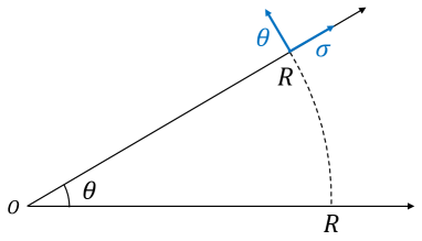
Figure 1: The polar coordinates in the field-space of the quasi-single field inflation.

Let us now decompose the metric through the ADM formalism [26] as

$$ds^{2}=-N^{2}dt^{2}+h_{ij}(dx^{i}+N^{i}dt)(dx^{j}+N^{j}dt).$$ (2.9)

Note that $h_{ij}$ is the spatial metric

$$\begin{split}&h_{ij}=a^{2}(t)e^{2\zeta}\left[\delta_{ij}+\gamma_{ij}+\frac{1}{2}\gamma_{il}\gamma_{lj}+\cdots\right],\end{split}$$ (2.10)

and that $N$ and $N^{i}$ are called ‘lapse’ and ‘shift’, respectively. The tensor fluctuation $\gamma_{ij}$ in (2.10) obeys transverse and traceless conditions, i.e., $\partial_{i}\gamma_{ij}=0,\gamma_{ii}=0$. The Einstein-Hilbert action together with the matter part (2.3) in this ADM language turns out to be

$$S=\frac{1}{2}\int d^{4}x\sqrt{h}\left[N\left(R^{(3)}+2\mathcal{L}_{m}\right)+N^{-1}\left(E_{ij}E^{ij}-E^{2}\right)\right],$$ (2.11)

where $R^{(3)}$ is the spatial scalar curvature and

$$E_{ij} \equiv \frac{1}{2}(\dot{h}_{ij}-\nabla_{i}N_{j}-\nabla_{j}N_{i}),$$ (2.12)

$$E \equiv E^{i}_{i}.$$ (2.13)

Note that ${\cal L}_{m}$ has been defined in (2.3). Then, setting $N=:1+N_{1}$ and solving the constraint equations

$$\frac{\delta S}{\delta N}=0,\quad\frac{\delta S}{\delta N^{j}}=0,$$ (2.14)

to the first order, we obtain

$$N_{1} = \frac{\dot{\zeta}}{H},$$ (2.15)

$$\partial_{i}N^{i} = -a^{-2}\frac{1}{H}\partial^{2}\zeta+\epsilon\left(\dot{\zeta}-\frac{2H}{R}\sigma\right).$$ (2.16)

The slow-roll parameter $\epsilon$ becomes $\epsilon\equiv-\dot{H}/H^{2}=R^{2}\dot{\theta}_{0}^{2}/2H^{2}$, according to (2.5).

Substituting (2.15) and (2.16) into the action (2.11) and performing some integrations by parts, we arrive at

$$S_{2} \equiv S_{\zeta\zeta}+S_{\gamma\gamma}+S_{\sigma\sigma}+\int d^{4}x\biggl{[}-2a^{3}(t)\frac{R\dot{\theta}_{0}^{2}}{H}\dot{\zeta}\,\sigma\biggl{]}.$$ (2.17)

for the quadratic part of the action, where

$$S_{\zeta\zeta} = \int d^{4}x\epsilon\left[a^{3}(t)\dot{\zeta}^{2}-a(t)(\partial\zeta)^{2}\right],$$ (2.18)

$$S_{\gamma\gamma} = \frac{1}{8}\int d^{4}x\left[a^{3}(t)\dot{\gamma}_{ij}\dot{\gamma}_{ij}-a(t)\partial_{l}\gamma_{ij}\partial_{l}\gamma_{ij}\right],$$ (2.19)

$$S_{\sigma\sigma} = \int d^{4}x\biggl{[}\frac{1}{2}a^{3}(t)(\dot{\sigma})^{2}-\frac{1}{2}a(t)(\partial\sigma)^{2}-\frac{1}{2}a^{3}(t)\left(V^{\prime\prime}(\chi_{0})-\dot{\theta}_{0}^{2}\right)(\sigma)^{2}\biggr{]}.$$ (2.20)

The third term in (2.20) is identified as the mass term of $\sigma$, i.e.,

$$m^{2}\equiv V^{\prime\prime}(\chi_{0})-\dot{\theta}_{0}^{2}\>.$$ (2.21)

The fourth term in (2.17) is a mixing interaction between $\zeta$ and $\sigma$, giving rise to corrections to the power spectrum of $\zeta$. Eqs. (2.18) and (2.19) indicate that the propagation velocities of scalar and tensor perturbations are both unity in the current treatment.

2.2 Effective field theory approach

Now that we have explained the quasi-single field inflation of Ref. [10], we would like to deal with it in a more general way by applying ideas of the EFT. Following the method of Ref. [3], we start from the unitary gauge and then employ the Stückelberg trick, i.e., translation in time direction,

$$t\to{\tilde{t}},\qquad\qquad t={\tilde{t}}+\pi({\tilde{t}},\mbox{\boldmath$x$}),$$ (2.22)

while the spatial coordinates $x^{i}$ are unchanged. The contravariant components of the metric transform under (2.22) as

$$g^{\rho\sigma} = \frac{\partial x^{\rho}}{\partial\tilde{x}^{\mu}}\frac{\partial x^{\sigma}}{\partial\tilde{x}^{\nu}}\tilde{g}^{\mu\nu}\>,$$ (2.23)

or more explicitly

$$g^{00} = (1+\dot{\pi})^{2}\tilde{g}^{00}+2(1+\dot{\pi})(\partial_{i}\pi)\tilde{g}^{0i}+(\partial_{i}\pi)(\partial_{j}\pi)\tilde{g}^{ij}\>,$$ (2.24)

$$g^{0i} = {\tilde{g}}^{0i}+{\dot{\pi}}{\tilde{g}}^{0i}+(\partial_{j}\pi){\tilde{g}}^{ji}\>,$$

$$g^{ij} = {\tilde{g}}^{ij}\>,$$

where the dot means $d/d{\tilde{t}}$. In the EFT, the $\pi$ field is regarded as the Nambu-Goldstone mode and one can go over to the spatially flat gauge by this transformation.

The action that we are going to work with in the unitary gauge is given by

$$S=S_{0}+S_{\sigma}+S_{I},$$ (2.25)

where

$$S_{0} = \int d^{4}x\sqrt{-g}\left[\frac{1}{2}R+\dot{H}(t)g^{00}-\left(3H^{2}(t)+\dot{H}(t)\right)\right],$$ (2.26)

$$S_{\sigma} = \int d^{4}x\sqrt{-g}\left[-\frac{1}{2}g^{\mu\nu}\partial_{\mu}\sigma\partial_{\nu}\sigma-\frac{1}{2}m^{2}\sigma^{2}+\cdots\right],$$ (2.27)

$$S_{I} = \int d^{4}x\sqrt{-g}\left[c_{1}\delta g^{00}\sigma+c_{2}(\delta g^{00})^{2}\sigma+c_{3}\delta g^{00}\sigma^{2}+c_{4}\delta g^{00}g^{\mu\nu}\partial_{\mu}\partial_{\nu}\sigma\right].$$ (2.28)

Note that $S_{0}$ is the standard part in the EFT action. (The reader should not confuse the scalar curvature $R$ in (2.26) with the radius $R={\tilde{R}}+\chi_{0}$ introduced previously.) In principle we can think of terms containing

$$\delta g^{00}\equiv g^{00}+1$$ (2.29)

and higher powers thereof without $\sigma$ field in (2.26). We are, however, interested in effects due to the heavy fields $\sigma$ in the present work, and so we do not include them in (2.26). In (2.27) the mass of $\sigma$ is denoted by $m$ and the ellipses $\cdots$ correspond to terms coming from $\sigma$’s potential $V(\sigma)$. The last one, $S_{I}$, shows the interaction of $\delta g^{00}$ and $\sigma$. The first three terms inside the pair of square brackets in (2.28) will be seen to produce terms which contain only $\zeta$ and $\sigma$ to the third order. In the unitary gauge, we could consider many more terms such as $\delta g^{00}\partial_{\mu}\sigma\partial^{\mu}\sigma$, $(\delta g^{00})^{2}\partial^{0}\sigma$ and so on so forth, but we will neglect these terms because they would contribute to the correlation functions (1.2) only at the loop level. The fourth term inside the pair of square brackets in (2.28) will be playing an important role in the present work because it produces a $\gamma\zeta\sigma$ coupling with the graviton coming from $g^{\mu\nu}$. We assume that all of the coefficients $c_{1}$, $c_{2}$, $c_{3}$ and $c_{4}$ are position-independent constants but may in principle be time-dependent. In later calculations, however, we understand that these coefficients are those at the time of horizon crossing. We could have included variations of the extrinsic curvature $K_{\mu\nu}$ in the most general setting. We, however, do not take those terms into account in the present work in order to avoid too much complication.

We are now in a position to perform the time diffeomorphism (2.22). Namely let us substitute $t=:\tilde{t}+\pi(\tilde{t},\mbox{\boldmath$x$})$ and use (2.24) for $g^{00}$ and (2.29) for $\delta g^{00}$. We then solve the constraint equations as we did in (2.14). To the first order, we can easily solve them and get (dropping all tildes):

$$N_{1} = -\epsilon\left(-H\pi\right),$$ (2.30)

$$\partial_{i}N^{i} = \epsilon\frac{d}{dt}\left(-H\pi\right)+c_{1}\frac{\sigma}{H}.$$ (2.31)

We now see a $\sigma$-dependent term in (2.31). Then, substituting these solutions into the action (2.25), and rewriting $\pi$ as

$$\pi=-\frac{\zeta}{H}\>,$$ (2.32)

we can finally obtain the action in terms of $\gamma$, $\zeta$ and $\sigma$. The action for the part of $\zeta$ and $\gamma$ is the same as Maldacena’s and the quadratic terms of the action, in particular, are given by $S_{\zeta\zeta}$ as in (2.18) and $S_{\gamma\gamma}$ as in (2.19), respectively. Note that the velocities of scalar and tensor fluctuations both turn out to be unity in the present work. The quadratic part of the $\sigma$ field is also the same as (2.20) under the relation (2.21), i.e.,

$$S_{\sigma\sigma} = \int d^{4}x\left[\frac{1}{2}a^{3}(t)\dot{\sigma}^{2}-\frac{1}{2}a(t)(\partial\sigma)^{2}-\frac{1}{2}a^{3}(t)m^{2}\sigma^{2}\right].$$ (2.33)

The new term including both $\zeta$ and $\sigma$ is

$$S_{\zeta\sigma} = \int d^{4}x\left[2\frac{c_{1}}{H}a^{3}(t)\dot{\zeta}\sigma\right].$$ (2.34)

As for the cubic action, the expansion gives rise to a lot of terms involving combinations of $\zeta$ and $\sigma$ such as $\zeta\sigma\sigma$ or $\zeta\zeta\sigma$, but as mentioned before, we will just examine a $\gamma\zeta\sigma$ coupling which is produced from the fourth term in (2.28):

$$S_{\gamma\zeta\sigma}=\int d^{4}x\left[-2\frac{c_{4}}{H}a(t)\dot{\zeta}\gamma_{ij}\partial_{i}\partial_{j}\sigma\right].$$ (2.35)

2.3 Quasi-single field inflation versus EFT

Let us check quickly how the set-up in the EFT is related to the quasi-single field inflation. We use again the uniform inflaton gauge (LABEL:uniforminflaton) in which the action (2.3) becomes

$$\begin{split}S_{m}=\int d^{4}x\sqrt{-g}\biggl{[}-\frac{1}{2}&\left(R+\sigma\right)^{2}g^{00}\,\dot{\theta}_{0}^{2}\\ &-\frac{1}{2}g^{\mu\nu}\partial_{\mu}\sigma\partial_{\nu}\sigma-V_{\textrm{sr}}(\theta_{0})-V(\chi_{0}+\sigma)\biggl{]}.\end{split}$$ (2.36)

Expanding the potential $V(\chi)$ as

$$V(\chi_{0}+\sigma)=V(\chi_{0})+V^{\prime}(\chi_{0})\sigma+\frac{1}{2}V^{\prime\prime}(\chi_{0})\sigma^{2}+\frac{1}{6}V^{\prime\prime\prime}(\chi_{0})\sigma^{3}+\cdots,$$ (2.37)

and substituting (2.4), (2.5) and (2.7) into (2.36), we arrive at

$$\begin{split}S_{m}=\int&d^{4}x\sqrt{-g}\biggl{[}\dot{H}(t)g^{00}-\left(3H^{2}(t)+\dot{H}(t)\right)\\ &-\frac{1}{2}g^{\mu\nu}\partial_{\mu}\sigma\partial_{\nu}\sigma-\frac{1}{2}\left(V^{\prime\prime}(\chi_{0})-\dot{\theta}_{0}^{2}\right)\sigma^{2}-\frac{1}{6}V^{\prime\prime\prime}(\chi_{0})\sigma^{3}-\cdots\\ &\qquad\qquad-R\dot{\theta}_{0}^{2}\left(g^{00}+1\right)\sigma-\frac{1}{2}\dot{\theta}_{0}^{2}\left(g^{00}+1\right)\sigma^{2}\biggl{]}.\end{split}$$ (2.38)

The first line corresponds to $S_{0}$ (2.26) except for the gravity term. The second line corresponds to $S_{\sigma}$ (2.27), where $m^{2}\equiv V^{\prime\prime}(\chi_{0})-\dot{\theta}_{0}^{2}$. Finally the third line corresponds to $S_{I}$, i.e., (2.28), and in order to go back to the quasi-single field inflation we are led to set

$$c_{1}=-R\dot{\theta}_{0}^{2},\quad c_{2}=0,\quad c_{3}=-\frac{1}{2}\dot{\theta}_{0}^{2},\quad c_{4}=0.$$ (2.39)

It follows therefore that the quasi-single field inflation belongs to the general class of inflationary models offered by the EFT method.

In the present paper we would like to generalize the quasi-single field inflation model with the help of the EFT method by taking into account the $c_{1}$ and $c_{4}$ terms. The effects due to the $c_{2}$ terms on the other hand are assumed to be small and are simply neglected, which is in accordance with the original quasi-single field inflation. This implies that the diagram with $\zeta\zeta\sigma$ and $\gamma\gamma\sigma$ vertices is considered as subdominant. With this assumption the scope of our analyses is kept within a reasonable size. The $c_{3}$ term gives rise to $\zeta\sigma\sigma$ type interactions and would contribute to the correlations (1.2) and (1.3) only at higher orders containing $\sigma$-loops. For this reason the $c_{3}$ interactions are not considered in our work.

2.4 Quantization of the $\zeta$, $\gamma$ and $\sigma$ fields

Now we would like to quantize scalar and tensor fluctuations, $\zeta$ and $\gamma$ together with the $\sigma$ field. In the quantization procedure we will use the conformal time $\eta$ defined by $d\eta\equiv dt/a(t)$. If we assume that $\eta$ moves from $-\infty$ to $0$ when $t$ moves from $-\infty$ to $\infty$, it follows that

$$\eta=-\frac{1}{aH},$$ (2.40)

where we have ignored terms involving the slow-roll parameters. The vacuum is always assumed to be the Bunch-Davies vacuum.

Quantization of the $\zeta$ field

The equation of motion for $\zeta$ is seen from the action (2.18) as

$$\frac{d^{2}\zeta}{d\eta^{2}}-\frac{2}{\eta}\frac{d\zeta}{d\eta}-\partial^{2}\zeta=0.$$ (2.41)

Note that we are taking the de Sitter limit, in which $H$ is almost constant and $\epsilon\ll 1$. The way to quantize $\zeta$ is the same as the usual quantum field theoretical method [27]. First of all, we represent $\zeta$ using the Fourier transformation,

$$\color[rgb]{0,0,0}\zeta(\eta,\boldsymbol{x})=\int\frac{d^{3}k}{(2\pi)^{3}}\bigg{[}u_{k}(\eta)a_{\boldsymbol{k}}e^{i\boldsymbol{k}\cdot\boldsymbol{x}}+u_{k}^{*}(\eta)a_{\boldsymbol{k}}^{\dagger}e^{-i\boldsymbol{k}\cdot\boldsymbol{x}}\bigg{]}$$ (2.42)

where $u_{k}$ and $u_{k}^{*}$ are the solutions of EOM, (2.41) and $a_{\boldsymbol{k}}$ and $a_{\boldsymbol{k}}^{\dagger}$ are respectively the annihilation and creation operators. They satisfy the commutation relation:

$$\left[a_{\boldsymbol{k}},a_{\boldsymbol{k}^{\prime}}^{\dagger}\right]=(2\pi)^{3}\delta^{3}(\boldsymbol{k}-\boldsymbol{k}^{\prime}).$$ (2.43)

This equation together with the canonical commutation relation imposes the normalization conditions on $u_{k}$ and $u_{k}^{*}$, which turn out to be

$$u_{k}(\eta) = \frac{H}{\sqrt{4\epsilon k^{3}}}(1+ik\eta)e^{-ik\eta},$$ (2.44)

$$u_{k}^{*}(\eta) = \frac{H}{\sqrt{4\epsilon k^{3}}}(1-ik\eta)e^{ik\eta}.$$ (2.45)

It is straightforward to derive two-point function formulae,

$$\langle 0|\zeta(t,\mbox{\boldmath$x$})\zeta(t^{\prime},\mbox{\boldmath$x$}^{\prime})|0\rangle = \int\frac{d^{3}k}{(2\pi)^{3}}e^{i{\boldsymbol{k}}\cdot(\boldsymbol{x}-\boldsymbol{x}^{\prime})}\left[\frac{H^{2}}{4\epsilon k^{3}}(1+ik\eta)(1-ik\eta^{\prime})e^{ik(\eta^{\prime}-\eta)}\right],$$ (2.46)

$$\langle 0|\zeta(t,\mbox{\boldmath$x$})\dot{\zeta}(t^{\prime},\mbox{\boldmath$x$}^{\prime})|0\rangle = \int\frac{d^{3}k}{(2\pi)^{3}}e^{i\boldsymbol{k}\cdot(\boldsymbol{x}-\boldsymbol{x}^{\prime})}\left[-\frac{H^{3}}{4\epsilon k}(1+ik\eta)\eta^{\prime 2}e^{ik(\eta^{\prime}-\eta)}\right],$$ (2.47)

which will be useful in our later computation. Here $|0\rangle$ denotes the Bunch-Davis vacuum.

Quantization of the $\gamma$ field

We can quantize the graviton field $\gamma_{ij}$ in a similar way. Let us recall that the quadratic action of $\gamma_{ij}$ is given by (2.19) and the EOM for $\gamma_{ij}$ turns out to be of the same form as (2.41), i.e.,

$$\frac{d^{2}\gamma_{ij}}{d\eta^{2}}-\frac{2}{\eta}\frac{d\gamma_{ij}}{d\eta}-\partial^{2}\gamma_{ij}=0.$$ (2.48)

We now represent $\gamma_{ij}$ in the Fourier transform as

$$\gamma_{ij}(\eta,\mbox{\boldmath$x$})=\sum_{s=+,\times}\int\frac{d^{3}k}{(2\pi)^{3}}\epsilon_{ij}^{s}(k)\left[U_{k}(\eta)b^{s}_{\boldsymbol{k}}e^{i\boldsymbol{k}\cdot\boldsymbol{x}}+U_{k}^{*}(\eta)b_{\boldsymbol{k}}^{s\dagger}e^{-i\boldsymbol{k}\cdot\boldsymbol{x}}\right],$$ (2.49)

where $U_{k}$ and $U_{k}^{*}$ are the solutions of EOM (2.48) and are given by

$$U_{k}(\eta) = \frac{H}{\sqrt{k^{3}}}(1+ik\eta)e^{-ik\eta},$$ (2.50)

$$U_{k}^{*}(\eta) = \frac{H}{\sqrt{k^{3}}}(1-ik\eta)e^{ik\eta},$$ (2.51)

and $\epsilon_{ij}^{s}$ is the polarization tensor satisfying the transverse and traceless condition, $k^{i}\epsilon_{ij}=\epsilon_{ii}=0$. The orthonormality condition is set as $\epsilon_{ij}^{s}(k)\epsilon_{ij}^{s^{\prime}}(k)=2\delta_{ss^{\prime}}$. Also $b_{\boldsymbol{k}}^{s}$ and $b_{\boldsymbol{k}}^{s{\dagger}}$are the annihilation and creation operators of graviton, respectively and satisfy the commutation relation

$$\left[b_{\boldsymbol{k}}^{s},b_{\boldsymbol{k}^{\prime}}^{s^{\prime}\dagger}\right]=(2\pi)^{3}\delta^{3}(\boldsymbol{k}-\boldsymbol{k}^{\prime})\delta_{ss^{\prime}}.$$ (2.52)

The two-point functions are easily worked out as

$$\langle 0|\gamma_{ij}(t,\mbox{\boldmath$x$})\gamma_{\alpha\beta}(t^{\prime},\mbox{\boldmath$x$}^{\prime})|0\rangle = \sum_{s}\int\frac{d^{3}q}{(2\pi)^{3}}e^{i\boldsymbol{q}\cdot(\boldsymbol{x}-\boldsymbol{x}^{\prime})}\epsilon_{ij}^{s}\epsilon_{\alpha\beta}^{s}\left[\frac{H^{2}}{q^{3}}(1+iq\eta)(1-iq\eta^{\prime})e^{iq(\eta^{\prime}-\eta)}\right],$$

$$\langle 0|\gamma_{ij}(t,\mbox{\boldmath$x$})\dot{\gamma}_{\alpha\beta}(t^{\prime},\mbox{\boldmath$x$}^{\prime})|0\rangle = \sum_{s}\int\frac{d^{3}q}{(2\pi)^{3}}e^{i\boldsymbol{q}\cdot(\boldsymbol{x}-\boldsymbol{x}^{\prime})}\epsilon_{ij}^{s}\epsilon_{\alpha\beta}^{s}\left[-\frac{H^{3}}{q}(1+iq\eta)\eta^{\prime 2}e^{iq(\eta^{\prime}-\eta)}\right].$$

Quantization of the $\sigma$ field

The quantization of $\sigma$ goes in the same way as $\zeta$. Firstly, we rewrite the quadratic action of $\sigma$ given in (2.33) by using the conformal time (2.40), and derive EOM

$$\frac{d^{2}\sigma}{d\eta^{2}}-\frac{2}{\eta}\frac{d\sigma}{d\eta}-\partial^{2}\sigma+\frac{m^{2}}{\eta^{2}H^{2}}\sigma=0.$$ (2.55)

Then we express $\sigma$ in the Fourier transform as

$$\sigma(\eta,\mbox{\boldmath$x$})=\int\frac{d^{3}{k}}{(2\pi)^{3}}\left[v_{k}(\eta)c_{\scriptsize{\mbox{\boldmath$k$}}}e^{i\boldsymbol{k}\cdot\boldsymbol{x}}+v_{k}^{*}(\eta)c_{\scriptsize{\mbox{\boldmath$k$}}}^{\dagger}e^{-i\boldsymbol{k}\cdot\boldsymbol{x}}\right],$$ (2.56)

where $v_{k}$ and $v_{k}^{*}$ are the solutions of EOM (2.55), and $c_{\boldsymbol{k}}$ and $c_{\boldsymbol{k}}^{\dagger}$ are the annihilation and creation operators respectively that satisfy the commutation relation given by

$$\left[c_{\boldsymbol{k}},c_{\boldsymbol{k}^{\prime}}^{\dagger}\right]=(2\pi)^{3}\delta^{3}(\boldsymbol{k}-\boldsymbol{k}^{\prime}).$$ (2.57)

The solutions to (2.55) are already known (the reader is referred to Ref. [28] for example) to be

$$v_{k}(\eta) = -ie^{i(\nu+\frac{1}{2})\frac{\pi}{2}}\frac{\sqrt{\pi}}{2}H(-\eta)^{3/2}H_{\nu}^{(1)}(-k\eta),$$ (2.58)

$$v_{k}^{*}(\eta) = ie^{-i(\nu^{*}+\frac{1}{2})\frac{\pi}{2}}\frac{\sqrt{\pi}}{2}H(-\eta)^{3/2}H_{\nu}^{(1)*}(-k\eta),$$ (2.59)

where

$$\nu\equiv\sqrt{\frac{9}{4}-\frac{m^{2}}{H^{2}}},$$ (2.60)

and $H_{\nu}^{(1)}$ is the Hankel function of the first kind. Using (2.56) with (2.58) and (2.59), we can compute the two point function of $\sigma$:

$$\langle 0|\sigma(\eta,\mbox{\boldmath$x$})\sigma(\eta^{\prime},\mbox{\boldmath$x$}^{\prime})|0\rangle$$

$$\qquad=\int\frac{d^{3}k}{(2\pi)^{3}}e^{i\boldsymbol{k}\cdot(\boldsymbol{x}-\boldsymbol{x}^{\prime})}\left[e^{-\pi\textrm{Im}(\nu)}\frac{\pi}{4}H^{2}(\eta\eta^{\prime})^{\frac{3}{2}}H_{\nu}^{(1)}(-k\eta)H_{\nu}^{(1)*}(-k\eta^{\prime})\right]$$ (2.61)

3 Computation of $\langle\zeta\zeta\rangle$, $\langle\gamma\zeta\zeta\rangle$, and $\langle\gamma\gamma\zeta\zeta\rangle$

We are now interested in the effects due to the interaction (2.28), in particular due to the terms of $c_{1}$ and $c_{4}$. Obviously these terms affect the power spectrum $\langle\zeta\zeta\rangle$ and the correlations $\langle\gamma\zeta\zeta\rangle$, $\langle\gamma\gamma\zeta\zeta\rangle$. The relevant Feynman diagrams are shown in Figure 2.

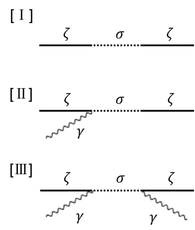
Figure 2: Effects due to the heavy field $\sigma$ on [I]  $\langle\zeta\zeta\rangle$, [II]   $\langle\gamma\zeta\zeta\rangle$ and [III]  $\langle\gamma\gamma\zeta\zeta\rangle$

The effect due to Figure 2 [I] has already been considered by Chen and Wang in their quasi-single field model [29]. In the following, we would like to generalize their method to compute also Figure 2 [II] and Figure 2 [III]. For this purpose we will use the in-in formalism [30, 31, 32], in which the expectation value of a certain operator $\mathcal{O}(t,\mbox{\boldmath$x$})$ can be computed by the formula

$$\langle\mathcal{O}(t,\mbox{\boldmath$x$})\rangle = \langle 0|\overline{T}\left[\textrm{exp}\left[i\int_{-\infty}^{\infty}dt^{\prime}H_{I}^{-}(t^{\prime})\right]\right]T\left[\mathcal{O}^{+}(t,\mbox{\boldmath$x$})\textrm{exp}\left[-i\int_{-\infty}^{\infty}dt^{\prime}H_{I}^{+}(t^{\prime})\right]\right]|0\rangle\>.$$

(3.1)

Here we label the interaction Hamiltonian $H_{I}$ and the operator $\mathcal{O}$ with ‘$+$’ or ‘$-$’ according to whether these operators are on the ‘$+$ path’ or ‘$-$ path’ as shown in Figure 3. Notice that on the $+$ path, operators are put in the usual time-ordering $(T)$, but on the $-$ path, operators are put in the anti-time ordering ($\overline{T}$). By shuffling Eq. (3.1), we are led to a more concise formula in the second order

$$\begin{split}&\langle\mathcal{O}(t,\mbox{\boldmath$x$})\rangle\Big{|}_{{\rm 2nd.\;order}}\\ &\qquad=\int_{-\infty}^{t}dt_{1}\int_{-\infty}^{t}dt_{2}\langle 0|H_{I}(t_{1})\mathcal{O}(t,\mbox{\boldmath$x$})H_{I}(t_{2})|0\rangle\\ &\qquad\qquad-2\textrm{Re}\left[\int_{-\infty}^{t}dt_{1}\int_{-\infty}^{t_{1}}dt_{2}\langle 0|\mathcal{O}(t,\mbox{\boldmath$x$})H_{I}(t_{1})H_{I}(t_{2})|0\rangle\right].\end{split}$$ (3.2)

Here $\mathcal{O}(t,\mbox{\boldmath$x$})$ is supposed to be either $\zeta\zeta$, $\gamma\zeta\zeta$ or $\gamma\gamma\zeta\zeta$.

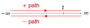
Figure 3: Time path in the in-in formalism.

3.1 Computation of $\langle\zeta\zeta\rangle$

The interaction Hamiltonian $H_{I}(t)=-L_{I}(t)$ relevant to Figure 2 [I] is given by the action (2.34):

$$H_{I}(t)\Big{|}_{{\rm Fig.}\>\ref{diagrams}\>[{\rm I}]}=-2\frac{c_{1}}{H}a^{3}(t)\int d^{3}x\,\dot{\zeta}\sigma.$$ (3.3)

Upon employing the two point functions (2.46), (2.47) and (2.61), we find for (3.2) with ${\cal O}=\zeta\zeta$

$$\begin{split}&\langle\zeta(\mbox{\boldmath$k$}_{1})\zeta(\mbox{\boldmath$k$}_{2})\rangle\Big{|}_{{\rm Fig.}\>\ref{diagrams}\>[\rm{I}]}\\ &=(2\pi)^{3}\delta^{3}(\mbox{\boldmath$k$}_{1}+\mbox{\boldmath$k$}_{2})\\ &\qquad\times\left(-2\frac{c_{1}}{H}\right)^{2}\left(-\frac{H^{3}}{4\epsilon k_{1}}\right)\left(-\frac{H^{3}}{4\epsilon k_{2}}\right)e^{-\pi\textrm{Im}(\nu)}\frac{\pi}{4}H^{2}\,\times\,2!\\ &\qquad\times\Biggl{[}\int_{-\infty}^{0}\frac{d\eta_{1}}{\eta_{1}^{4}H^{4}}\int_{-\infty}^{0}\frac{d\eta_{2}}{\eta_{2}^{4}H^{4}}\eta_{1}^{2}e^{-ik_{1}\eta_{1}}\eta_{2}^{2}e^{ik_{2}\eta_{2}}(\eta_{1}\eta_{2})^{\frac{3}{2}}H_{\nu}^{(1)}(-k_{2}\eta_{1})H_{\nu}^{(1)*}(-k_{2}\eta_{2})\\ &\qquad-2\textrm{Re}\left[\int_{-\infty}^{0}\frac{d\eta_{1}}{\eta_{1}^{4}H^{4}}\int_{-\infty}^{\eta_{1}}\frac{d\eta_{2}}{\eta_{2}^{4}H^{4}}\eta_{1}^{2}e^{ik_{1}\eta_{1}}\eta_{2}^{2}e^{ik_{2}\eta_{2}}(\eta_{1}\eta_{2})^{\frac{3}{2}}H_{\nu}^{(1)}(-k_{2}\eta_{1})H_{\nu}^{(1)*}(-k_{2}\eta_{2})\right]\Biggl{]}.\end{split}$$ (3.4)

The factor ‘$\times\,2!$’ in the third line in (3.4) is a combinatorial factor.

We now evaluate (3.4) at $t\to\infty$, which corresponds to $\eta\to 0$. If we set $x\equiv-k_{2}\eta_{1}$ and $y\equiv-k_{2}\eta_{2}$, then (3.4) becomes

$$\begin{split}&\langle\zeta(\mbox{\boldmath$k$}_{1})\zeta(\mbox{\boldmath$k$}_{2})\rangle\Big{|}_{{\rm Fig.}\>\ref{diagrams}\>[\rm{I}]}\\ &=(2\pi)^{3}\delta^{3}(\mbox{\boldmath$k$}_{1}+\mbox{\boldmath$k$}_{2})\ P_{\zeta}(k_{2})\ \frac{\pi c_{1}^{2}}{2\epsilon H^{4}}e^{-\pi\textrm{Im}(\nu)}\\ &\qquad\times\Biggl{[}\left|\int_{0}^{\infty}dx\ x^{-\frac{1}{2}}e^{ix}H_{\nu}^{(1)}(x)\right|^{2}\\ &\qquad\quad-2\textrm{Re}\left[\int_{0}^{\infty}dx\ x^{-\frac{1}{2}}e^{-ix}H_{\nu}^{(1)}(x)\int_{x}^{\infty}dy\ y^{-\frac{1}{2}}e^{-iy}H_{\nu}^{(1)*}(y)\right]\Biggl{]},\end{split}$$ (3.5)

where

$$P_{\zeta}(k)=\frac{H^{2}}{4\epsilon k^{3}}\>.$$ (3.6)

would be the power spectrum of the scalar perturbation in the absence of the heavy field $\sigma$.

The integrations in (3.5) are worked out in Appendices A and B and in fact by putting (A.6) and (B.17) in (3.5) we arrive at the following formula

$$\begin{split}\langle&\zeta(\mbox{\boldmath$k$}_{1})\zeta(\mbox{\boldmath$k$}_{2})\rangle\Big{|}_{{\rm Fig.\>\ref{diagrams}\>(I)}}=(2\pi)^{3}\delta^{3}(\mbox{\boldmath$k$}_{1}+\mbox{\boldmath$k$}_{2})\,P_{\zeta}(k_{2})\,\frac{c_{1}^{2}}{\epsilon H^{4}}F_{1}(m),\end{split}$$ (3.7)

where

$$F_{1}(m) \equiv \frac{\pi^{2}}{\textrm{cosh}^{2}(\pi\mu)}-\frac{1}{\textrm{sinh}(\pi\mu)}\textrm{Re}\left[\sum_{n=0}^{\infty}(-1)^{n}\Biggl{\{}\frac{e^{\pi\mu}}{(\frac{1}{2}+n+i\mu)^{2}}-\frac{e^{-\pi\mu}}{(\frac{1}{2}+n-i\mu)^{2}}\Biggl{\}}\right],$$

(3.8)

with

$$\mu\equiv\sqrt{\frac{m^{2}}{H^{2}}-\frac{9}{4}}=-i\nu\>.$$ (3.9)

In the course of deriving the formula (3.8), we assumed that $\mu$ is real, namely, $m/H>3/2$. The function $F_{1}(m)$, however, can be continued to the region $m/H<3/2$ smoothly and its shape is as depicted in Figure 4.

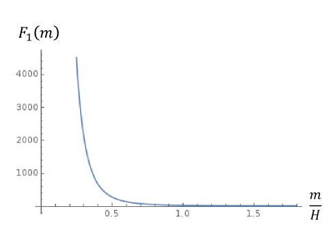
Figure 4: The plot for $F_{1}(m)$ with $m>0$

Note that the function $F_{1}(m)$ has previously been evaluated numerically by Chen and Wang [29] and our calculation is in good agreement with theirs. An approximate analytic formula for $F_{1}(m)$ has also been studied in Ref. [17].

3.2 Computation of $\langle\gamma\zeta\zeta\rangle$ in the soft graviton limit

The interaction Hamiltonian relevant to Figure 2 [II] consists of two terms, namely, one from (2.34) and the other from (2.35):

$$H_{I}(t)\Big{|}_{{\rm Fig.}\>\ref{diagrams}\>[{\rm II}]}=-2\frac{c_{1}}{H}a^{3}(t)\int d^{3}x\,\dot{\zeta}\sigma+2\frac{c_{4}}{H}a(t)\int d^{3}x\,\dot{\zeta}\gamma_{ij}\partial_{i}\partial_{j}\sigma.$$ (3.10)

Using the two point functions (2.46), (2.47) and (2.61), we find the formula (3.2) with $\mathcal{O}=\gamma\zeta\zeta$ turns out to be

$$\begin{split}&\langle\gamma^{s}(\mbox{\boldmath$q$})\zeta(\mbox{\boldmath$k$}_{1})\zeta(\mbox{\boldmath$k$}_{2})\rangle\Big{|}_{{\rm Fig.\>\ref{diagrams}\>[II]}}\\ &=(2\pi)^{3}\delta^{3}(\mbox{\boldmath$q$}+\mbox{\boldmath$k$}_{1}+\mbox{\boldmath$k$}_{2})\ \epsilon_{ij}^{s}(\mbox{\boldmath$q$})(-i)^{2}(k_{2})_{i}(k_{2})_{j}\\ &\qquad\times\left(-4\frac{c_{1}c_{4}}{H^{2}}\right)\frac{H^{2}}{q^{3}}\left(-\frac{H^{3}}{4\epsilon k_{1}}\right)\left(-\frac{H^{3}}{4\epsilon k_{2}}\right)e^{-\pi\textrm{Im}(\nu)}\frac{\pi}{4}H^{2}\,\times\,2!\\ &\qquad\times\Biggl{[}2\textrm{Re}\left[\int_{-\infty}^{0}\frac{d\eta_{1}}{\eta_{1}^{4}H^{4}}\int_{-\infty}^{0}\frac{d\eta_{2}}{\eta_{2}^{2}H^{2}}\eta_{1}^{2}e^{-ik_{1}\eta_{1}}\eta_{2}^{2}e^{ik_{2}\eta_{2}}(\eta_{1}\eta_{2})^{\frac{3}{2}}H_{\nu}^{(1)}(-k_{2}\eta_{1})H_{\nu}^{(1)*}(-k_{2}\eta_{2})\right]\\ &\quad\qquad-2\textrm{Re}\left[\int_{-\infty}^{0}\frac{d\eta_{1}}{\eta_{1}^{4}H^{4}}\int_{-\infty}^{\eta_{1}}\frac{d\eta_{2}}{\eta_{2}^{2}H^{2}}\eta_{1}^{2}e^{ik_{1}\eta_{1}}\eta_{2}^{2}e^{ik_{2}\eta_{2}}(\eta_{1}\eta_{2})^{\frac{3}{2}}H_{\nu}^{(1)}(-k_{2}\eta_{1})H_{\nu}^{(1)*}(-k_{2}\eta_{2})\right]\\ &\quad\qquad-2\textrm{Re}\left[\int_{-\infty}^{0}\frac{d\eta_{1}}{\eta_{1}^{2}H^{2}}\int_{-\infty}^{\eta_{1}}\frac{d\eta_{2}}{\eta_{2}^{4}H^{4}}\eta_{1}^{2}e^{ik_{1}\eta_{1}}\eta_{2}^{2}e^{ik_{2}\eta_{2}}(\eta_{1}\eta_{2})^{\frac{3}{2}}H_{\nu}^{(1)}(-k_{2}\eta_{1})H_{\nu}^{(1)*}(-k_{2}\eta_{2})\right]\Biggl{]}.\end{split}$$ (3.11)

Note that we have already taken the $\mbox{\boldmath$q$}\to 0$ limit to simplify our mathematical manipulation, and so $q$ does not appear in the above integrals. The factor ‘$\times\,2!$’ in the third line of (3.11) is again a combinatorial factor.

By setting $x\equiv-k_{2}\eta_{1}$ and $y\equiv-k_{2}\eta_{2}$, (3.11) may be transformed into

$$\begin{split}&\langle\gamma^{s}(\mbox{\boldmath$q$})\zeta(\mbox{\boldmath$k$}_{1})\zeta(\mbox{\boldmath$k$}_{2})\rangle\Big{|}_{{\rm Fig.\>\ref{diagrams}\>[II]}}\\ &=(2\pi)^{3}\delta^{3}(\mbox{\boldmath$q$}+\mbox{\boldmath$k$}_{1}+\mbox{\boldmath$k$}_{2})\ \epsilon_{ij}^{s}(\mbox{\boldmath$q$})\frac{(k_{2})_{i}(k_{2})_{j}}{(k_{2})^{2}}P_{\gamma}(q)P_{\zeta}(k_{2})\frac{\pi c_{1}c_{4}}{\epsilon H^{2}}e^{-\pi\textrm{Im}(\nu)}\\ &\qquad\times\Biggl{[}\textrm{Re}\left[\int_{0}^{\infty}dx\ x^{-\frac{1}{2}}e^{ix}H_{\nu}^{(1)}(x)\int_{0}^{\infty}dy\ y^{\frac{3}{2}}e^{-iy}H_{\nu}^{(1)*}(y)\right]\\ &\qquad\qquad-\textrm{Re}\left[\int_{0}^{\infty}dx\ x^{-\frac{1}{2}}e^{-ix}H_{\nu}^{(1)}(x)\int_{x}^{\infty}dy\ y^{\frac{3}{2}}e^{-iy}H_{\nu}^{(1)*}(y)\right]\\ &\qquad\qquad-\textrm{Re}\left[\int_{0}^{\infty}dx\ x^{\frac{3}{2}}e^{-ix}H_{\nu}^{(1)}(x)\int_{x}^{\infty}dy\ y^{-\frac{1}{2}}e^{-iy}H_{\nu}^{(1)*}(y)\right]\Biggl{]},\end{split}$$ (3.12)

where

$$P_{\gamma}(q)=\frac{H^{2}}{q^{3}}\>.$$ (3.13)

would be the power spectrum of the tensor perturbation in the absence of $\sigma$. (Note in passing that this may differ from the formula often found in literatures by factor four.)

The reader is referred to Appendices A and B for the integration formulas for (3.12). By combining (A.6), (A.8), (B.19), and (B.18) altogether in (3.12) one can easily find a formula

$$\begin{split}\langle\gamma^{s}&(\mbox{\boldmath$q$})\zeta(\mbox{\boldmath$k$}_{1})\zeta(\mbox{\boldmath$k$}_{2})\rangle\Big{|}_{{\rm Fig.\>\ref{diagrams}\>[II]}}\\ &=(2\pi)^{3}\delta^{3}(\mbox{\boldmath$q$}+\mbox{\boldmath$k$}_{1}+\mbox{\boldmath$k$}_{2})\ \epsilon_{ij}^{s}(\mbox{\boldmath$q$})\frac{(k_{2})_{i}(k_{2})_{j}}{(k_{2})^{2}}P_{\gamma}(q)P_{\zeta}(k_{2})\frac{c_{1}c_{4}}{\epsilon H^{2}}\,F_{2}(m),\end{split}$$ (3.14)

where we have introduced the following function

$$\begin{split}F_{2}(m)\equiv&-\frac{1}{4}\left(\frac{1}{4}+\mu^{2}\right)\left(\frac{9}{4}+\mu^{2}\right)\frac{\pi^{2}}{\textrm{cosh}^{2}(\pi\mu)}\\ &\quad\quad+\frac{1}{2\,\textrm{sinh}(\pi\mu)}\,\textrm{Re}\Biggl{[}\,\sum_{n=0}^{\infty}(-1)^{n}(n+1)(n+2)\\ &\qquad\qquad\qquad\qquad\qquad\times\Biggl{\{}e^{\pi\mu}\frac{(1+n+2i\mu)(2+n+2i\mu)}{(\frac{1}{2}+n+i\mu)^{2}(\frac{5}{2}+n+i\mu)^{2}}\\ &\qquad\qquad\qquad\qquad\qquad\qquad-e^{-\pi\mu}\frac{(1+n-2i\mu)(2+n-2i\mu)}{(\frac{1}{2}+n-i\mu)^{2}(\frac{5}{2}+n-i\mu)^{2}}\Biggl{\}}\Biggl{]},\end{split}$$ (3.15)

Recall that the quantity $\mu$ has been introduced in (3.9).

We have to pay a careful attention to the summation over $n$ in (3.15). Because of the factor $(-1)^{n}$, it is an alternating sum, but the large $n$ behavior of each term is not mild enough to confirm the convergence. The source of this indefinite nature of the summation may be traced back to the oscillatory behavior of the Hankel functions in (3.12) for large $x$ and large $y$ and the factor $x^{3/2}$ and/or $y^{3/2}$. We may regularize the integrals in (3.12) by deforming the integration paths slightly away from the real axis on the complex $x$ and $y$ planes so that the integrals should converge. This type of regularization would lead us eventually to the regularization of the indefinite sum in (3.15), such as zeta-function regularization. In the actual numerical calculation of $F_{2}(m)$, we assume that we are allowed to make use of the zeta-function regularization method in the summation in (3.15). We will also employ the zeta-function regularization in subsequent calculations in the present paper. The function $F_{2}(m)$ thus regularizaed is shown in Figure 5, which looks as if it were decreasing monotonically as the mass $m$ becomes large. This is, however, not the case. In fact $F_{2}(m)$ has a local minimum at $m/H\sim$ 2.3, which is outside in Figure 5. We will come to this point later, when we illustrate $F_{2}(m)$ in a different region of $m/H$ in Figure 7.

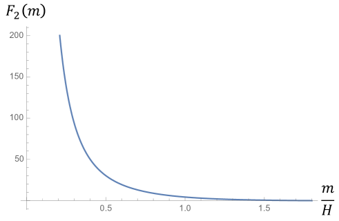
Figure 5: The plot for $F_{2}(m)$ with $m>0$

3.3 Computation of $\langle\gamma\gamma\zeta\zeta\rangle$ in the soft graviton limit

The interaction Hamiltonian that is necessary to evaluate Figure 2 [III] is given simply by (2.35):

$$H_{I}(t)\Big{|}_{{\rm Fig.}\>\ref{diagrams}\>[{\rm III}]}=2\frac{c_{4}}{H}a(t)\int d^{3}x\,\dot{\zeta}\gamma_{ij}\partial_{i}\partial_{j}\sigma.$$ (3.16)

A straightforward application of the two-point functions given previously provides us with the formula (3.2) with $\mathcal{O}=\gamma\gamma\zeta\zeta$ in the following way,

$$\begin{split}&\langle\gamma^{s_{1}}(\mbox{\boldmath$q$}_{1})\gamma^{s_{2}}(\mbox{\boldmath$q$}_{2})\zeta(\mbox{\boldmath$k$}_{1})\zeta(\mbox{\boldmath$k$}_{2})\rangle\Big{|}_{{\rm Fig.\>\ref{diagrams}\>[III]}}\\ &=(2\pi)^{3}\delta^{3}(\mbox{\boldmath$q$}_{1}+\mbox{\boldmath$q$}_{2}+\mbox{\boldmath$k$}_{1}+\mbox{\boldmath$k$}_{2})\ \epsilon_{ij}^{s_{1}}(\mbox{\boldmath$q$}_{1})(-i)^{2}(k_{1})_{i}(k_{1})_{j}\ \epsilon_{\alpha\beta}^{s_{2}}(\mbox{\boldmath$q$}_{2})(-i)^{2}(k_{2})_{\alpha}(k_{2})_{\beta}\\ &\qquad\times\left(2\frac{c_{4}}{H}\right)^{2}\frac{H^{2}}{(q_{1})^{3}}\frac{H^{2}}{(q_{2})^{3}}\left(-\frac{H^{3}}{4\epsilon k_{1}}\right)\left(-\frac{H^{3}}{4\epsilon k_{2}}\right)e^{-\pi\textrm{Im}(\nu)}\frac{\pi}{4}H^{2}\,\times\,2!\times 2!\\ &\qquad\times\Biggl{[}\int_{-\infty}^{0}\frac{d\eta_{1}}{\eta_{1}^{2}H^{2}}\int_{-\infty}^{0}\frac{d\eta_{2}}{\eta_{2}^{2}H^{2}}\eta_{1}^{2}e^{-ik_{1}\eta_{1}}\eta_{2}^{2}e^{ik_{2}\eta_{2}}(\eta_{1}\eta_{2})^{\frac{3}{2}}H_{\nu}^{(1)}(-k_{2}\eta_{1})H_{\nu}^{(1)*}(-k_{2}\eta_{2})\\ &\qquad-2\textrm{Re}\left[\int_{-\infty}^{0}\frac{d\eta_{1}}{\eta_{1}^{2}H^{2}}\int_{-\infty}^{\eta_{1}}\frac{d\eta_{2}}{\eta_{2}^{2}H^{2}}\eta_{1}^{2}e^{ik_{1}\eta_{1}}\eta_{2}^{2}e^{ik_{2}\eta_{2}}(\eta_{1}\eta_{2})^{\frac{3}{2}}H_{\nu}^{(1)}(-k_{2}\eta_{1})H_{\nu}^{(1)*}(-k_{2}\eta_{2})\right]\Biggl{]}.\end{split}$$ (3.17)

Note that we have already taken the double-soft limit $\mbox{\boldmath$q$}_{1},\mbox{\boldmath$q$}_{2}\to 0$ for the sake of calculational simplicity. The factor ‘$\times\,2!\times 2!$’ in the third line of (3.17) is, as before, a combinatorial factor for Figure 2 [III] .

If we change the integration variables from $\eta_{1}$ and $\eta_{2}$ into $x\equiv-k_{2}\eta_{1}$ and $y\equiv-k_{2}\eta_{2}$ respectively, then the correlation function (3.17) becomes

$$\begin{split}&\langle\gamma^{s_{1}}(\mbox{\boldmath$q$}_{1})\gamma^{s_{2}}(\mbox{\boldmath$q$}_{2})\zeta(\mbox{\boldmath$k$}_{1})\zeta(\mbox{\boldmath$k$}_{2})\rangle\Big{|}_{{\rm Fig.\>\ref{diagrams}\>[III]}}\\ &=(2\pi)^{3}\delta^{3}(\mbox{\boldmath$q$}_{1}+\mbox{\boldmath$q$}_{2}+\mbox{\boldmath$k$}_{1}+\mbox{\boldmath$k$}_{2})\\ &\qquad\times\epsilon_{ij}^{s_{1}}(\mbox{\boldmath$q$}_{1})\frac{(k_{2})_{i}(k_{2})_{j}}{(k_{2})^{2}}\epsilon_{\alpha\beta}^{s_{2}}(\mbox{\boldmath$q$}_{2})\frac{(k_{2})_{\alpha}(k_{2})_{\beta}}{(k_{2})^{2}}P_{\gamma}(q_{1})P_{\gamma}(q_{2})P_{\zeta}(k_{2})\frac{\pi c_{4}^{2}}{\epsilon}e^{-\pi\textrm{Im}(\nu)}\\ &\qquad\times\Biggl{[}\left|\int_{0}^{\infty}dx\ x^{\frac{3}{2}}e^{ix}H_{\nu}^{(1)}(x)\right|^{2}\\ &\qquad\qquad-2\textrm{Re}\left[\int_{0}^{\infty}dx\ x^{\frac{3}{2}}e^{-ix}H_{\nu}^{(1)}(x)\int_{x}^{\infty}dy\ y^{\frac{3}{2}}e^{-iy}H_{\nu}^{(1)*}(y)\right]\Biggl{]}.\end{split}$$ (3.18)

In order to look at the $m$-dependence of (3.18) more closely, we may put the integration formulae in (A.6) and (B.20) and then we end up with

$$\begin{split}&\langle\gamma^{s_{1}}(\mbox{\boldmath$q$}_{1})\gamma^{s_{2}}(\mbox{\boldmath$q$}_{2})\zeta(\mbox{\boldmath$k$}_{1})\zeta(\mbox{\boldmath$k$}_{2})\rangle\Big{|}_{{\rm Fig.\>\ref{diagrams}\>[III]}}\\ &\quad=(2\pi)^{3}\delta^{3}(\mbox{\boldmath$q$}_{1}+\mbox{\boldmath$q$}_{2}+\mbox{\boldmath$k$}_{1}+\mbox{\boldmath$k$}_{2})\\ &\qquad\quad\times\epsilon_{ij}^{s_{1}}(\mbox{\boldmath$q$}_{1})\frac{(k_{2})_{i}(k_{2})_{j}}{(k_{2})^{2}}\epsilon_{\alpha\beta}^{s_{2}}(\mbox{\boldmath$q$}_{2})\frac{(k_{2})_{\alpha}(k_{2})_{\beta}}{(k_{2})^{2}}P_{\gamma}(q_{1})P_{\gamma}(q_{2})P_{\zeta}(k_{2})\frac{c_{4}^{2}}{\epsilon}\,F_{3}(m),\end{split}$$ (3.19)

where the function $F_{3}(m)$ defined by

$$\begin{split}F_{3}&(m)\equiv\\ &\frac{1}{32}\left(\frac{1}{4}+\mu^{2}\right)^{2}\left(\frac{9}{4}+\mu^{2}\right)^{2}\frac{\pi^{2}}{\textrm{cosh}^{2}(\pi\mu)}\\ &-\frac{1}{8\,\textrm{sinh}(\pi\mu)}\\ &\quad\quad\times\textrm{Re}\Biggl{[}\,\sum_{n=0}^{\infty}(-1)^{n}(n+1)(n+2)(n+3)(n+4)\\ &\qquad\times\Biggl{\{}e^{\pi\mu}\frac{(1+n+2i\mu)(2+n+2i\mu)(3+n+2i\mu)(4+n+2i\mu)}{(\frac{1}{2}+n+i\mu)(\frac{3}{2}+n+i\mu)(\frac{5}{2}+n+i\mu)^{2}(\frac{7}{2}+n+i\mu)(\frac{9}{2}+n+i\mu)}\\ &\quad\qquad-e^{-\pi\mu}\frac{(1+n-2i\mu)(2+n-2i\mu)(3+n-2i\mu)(4+n-2i\mu)}{(\frac{1}{2}+n-i\mu)(\frac{3}{2}+n-i\mu)(\frac{5}{2}+n-i\mu)^{2}(\frac{7}{2}+n-i\mu)(\frac{9}{2}+n-i\mu)}\Biggl{\}}\Biggl{]}.\end{split}$$ (3.20)

has a peculiar behavior as is shown in Figure 6.

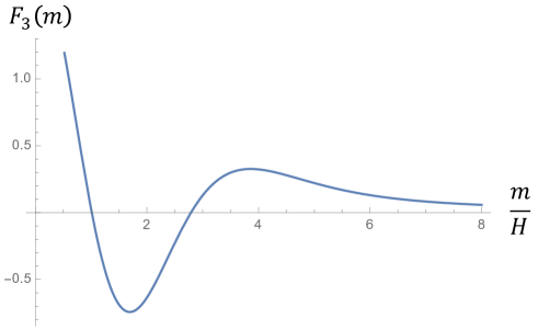
Figure 6: The plot for $F_{3}(m)$ in $m>0$

4 The large mass limit $m\to\infty$

Since we are interested in the signature of the heavy field $\sigma$ in the correlation functions, we would like to scrutinize the $m$-dependence of the three characteristic functions $F_{i}(m)\>\>\>(i=1,2,3)$ which are drawn together in Figure 7. Note that $F_{2}(m)$ has a local minimum around $m/H\sim 2.3$, which was not seen in Figure 5. While we can see local maxima and local minima in Figure 7, the three functions approach all to zero as $m\to\infty$. This is natural because heavy particle effects are in general expected to disappear at lower energy, which is in the present case the Hubble parameter $H$.

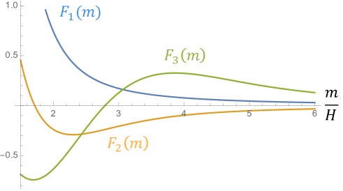
Figure 7: The plots for $F_{1}(m)$, $F_{2}(m)$ and $F_{3}(m)$ in $m\geq 1.5H$

Curiously, the rate by which $F_{1}(m)$, $F_{2}(m)$ and $F_{3}(m)$ approach the horizontal axis as $m\to\infty$ seems to be shared commonly by these three functions. In order to examine this point further, let us consider the ratios

$$G_{12}(m)\equiv\frac{F_{1}(m)}{F_{2}(m)},\quad G_{23}(m)\equiv\frac{F_{2}(m)}{F_{3}(m)}.$$ (4.1)

We have performed numerical analyses of these ratios by Mathematica 11, the result of which is given in Table 1 below:

Table 1: The numerical analysis of $G_{12}(m)$ and $G_{23}(m)$

$\displaystyle m/H$	$\displaystyle 5.0$	$\displaystyle 10.0$	$\displaystyle 15.0$	$\displaystyle 20.0$	$\displaystyle 25.0$	$\displaystyle 30.0$
$\displaystyle G_{12}(m)$	$\displaystyle-0.88031$	$\displaystyle-0.978412$	$\displaystyle-0.99082$	$\displaystyle-0.99491$	$\displaystyle-0.996764$	$\displaystyle-0.99776$
$\displaystyle G_{23}(m)$	$\displaystyle-0.233967$	$\displaystyle-0.310469$	$\displaystyle-0.323965$	$\displaystyle-0.328174$	$\displaystyle-0.330123$	$\displaystyle-0.331035$

This result suggests the limiting behavior

$$\lim_{m\to\infty}G_{12}(m)\to-1,\qquad\lim_{m\to\infty}G_{23}(m)\to-\frac{1}{3}.$$ (4.2)

Looking at the expressions (3.9), (3.15) and (3.20), we do not find it easy to work out explicitly the asymptotic behaviors of $F_{i}(m)\>(i=1,2,3)$ as $m\to\infty$. We are, however, able to determine the asymptotic values (4.2) by employing an alternative method.

Suppose that the mass of $\sigma$ is extremely large and the $\sigma$ field is integrated out. Then the interaction Hamiltonians relevant to the three diagrams in Figure 2 are reduced, by using (2.34) and (2.35), to

$$H_{I}(t)\Big{|}_{{\rm Fig.}\>\ref{effectivefigure}\>[{\rm I}]} = \left(-2\frac{c_{1}}{H}\right)^{2}a^{3}(t)f(m)\int d^{3}x\ \dot{\zeta}^{2},$$ (4.3)

$$H_{I}(t)\Big{|}_{{\rm Fig.}\>\ref{effectivefigure}\>[{\rm II}]} = \left(-2\frac{c_{1}}{H}\right)\left(2\frac{c_{4}}{H}\right)a(t)f(m)\int d^{3}x\ \dot{\zeta}\,\gamma_{ij}\partial_{i}\partial_{j}\dot{\zeta}\ \times 2,$$ (4.4)

$$H_{I}(t)\Big{|}_{{\rm Fig.}\>\ref{effectivefigure}\>[{\rm III}]} = \left(2\frac{c_{4}}{H}\right)^{2}a^{-1}(t)f(m)\int d^{3}x\ \gamma_{ij}\partial_{i}\partial_{j}\dot{\zeta}\,\gamma_{\alpha\beta}\partial_{\alpha}\partial_{\beta}\dot{\zeta}.$$ (4.5)

This simplification is illustrated in Figure 8. Note that $f(m)$ in (4.3), (4.4) and (4.5) is a certain common function of $m$. Incidentally we have to be careful about the power of $a(t)$ in (4.3), (4.4) and (4.5). The volume element of the integration of course gives us $\sqrt{-g}=a^{3}(t)$ in the action. In addition, the tensor perturbation $\gamma_{ij}$ is always accompanied by $a^{-2}(t)$ since $\gamma$ comes from the inverse spatial metric $h^{ij}$, which has $a^{-2}(t)$. This explains the power of $a(t)$ in (4.3), (4.4) and (4.5). Also note that we are allowed to impose $\partial_{i}\partial_{j}$, which operated on $\sigma$ in (2.35), on $\dot{\zeta}$ because in the soft-graviton limit, $\sigma$ and $\dot{\zeta}$ have the same momentum in the momentum space. Finally, notice that there is a factor ‘$2$’ in the last in (4.4) because there are two diagrams originally as Figure 8 [II] shows.

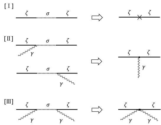
Figure 8: The original Feynman diagrams (left) are simplified into the right diagrams as $m\to\infty$

Since the simplified diagrams (those on the right hand side in Figure 8 ) have only one vertex, the computation is much easier than the original ones (left ones in Figure 8). Using the in-in formalism (3.1), the correlation function of $\mathcal{O}(t,\mbox{\boldmath$x$})$ ($=\zeta\zeta$, $\gamma\zeta\zeta$ and $\gamma\gamma\zeta\zeta$) in this case is given in the first order by

$$\langle 0(t)|\mathcal{O}(t,\mbox{\boldmath$x$})|0(t)\rangle\Big{|}_{{\rm 1st.\>order}}=2\,\textrm{Im}\left[\int_{-\infty}^{t}dt^{\prime}\ \langle 0|\mathcal{O}(t,\mbox{\boldmath$x$})H_{I}(t^{\prime})|0\rangle\right].$$ (4.6)

Putting the interaction Hamiltonian (4.3),(4.4) and (4.5) into (4.6) , and also using the two point functions discussed previously, we can reach the following simplified formulae:

$$\langle\zeta(\mbox{\boldmath$k$}_{1})\zeta(\mbox{\boldmath$k$}_{2})\rangle\Big{|}_{{\rm Fig.\>\ref{effectivefigure}\>[I]}} \Rightarrow \quad(2\pi)^{3}\delta^{3}(\mbox{\boldmath$k$}_{1}+\mbox{\boldmath$k$}_{2})$$ (4.7)

$$\qquad\times f(m)\left(-2\frac{c_{1}}{H}\right)^{2}\left(-\frac{H^{3}}{4\epsilon k_{1}}\right)\left(-\frac{H^{3}}{4\epsilon k_{2}}\right)\times\,2!$$

$$\qquad\qquad\times 2\,\textrm{Im}\left[\int_{-\infty}^{0}\frac{d\eta}{\eta^{4}H^{4}}\eta^{2}e^{ik_{1}\eta}\eta^{2}e^{ik_{2}\eta}\right]$$

$$= \quad(2\pi)^{3}\delta^{3}(\mbox{\boldmath$k$}_{1}+\mbox{\boldmath$k$}_{2})\,P_{\zeta}(k_{2})\,\frac{c_{1}^{2}}{\epsilon H^{4}}\tilde{F}_{1}(m),$$

$$\langle\gamma^{s}(\mbox{\boldmath$q$})\zeta(\mbox{\boldmath$k$}_{1})\zeta(\mbox{\boldmath$k$}_{2})\rangle\Big{|}_{{\rm Fig.\>\ref{effectivefigure}\>[II]}} \Rightarrow \quad(2\pi)^{3}\delta^{3}(\mbox{\boldmath$q$}+\mbox{\boldmath$k$}_{1}+\mbox{\boldmath$k$}_{2})\ \epsilon_{ij}^{s}(\mbox{\boldmath$q$})(-i)^{2}(k_{2})_{i}(k_{2})_{j}$$ (4.8)

$$\qquad\times f(m)\left(-4\frac{c_{1}c_{4}}{H^{2}}\right)\frac{H^{2}}{q^{3}}\left(-\frac{H^{3}}{4\epsilon k_{1}}\right)\left(-\frac{H^{3}}{4\epsilon k_{2}}\right)\times 2\,\times\,2!$$

$$\qquad\qquad\times 2\,\textrm{Im}\left[\int_{-\infty}^{0}\frac{d\eta}{\eta^{2}H^{2}}\eta^{2}e^{ik_{1}\eta}\eta^{2}e^{ik_{2}\eta}\right]$$

$$= \quad(2\pi)^{3}\delta^{3}(\mbox{\boldmath$q$}+\mbox{\boldmath$k$}_{1}+\mbox{\boldmath$k$}_{2})\ \epsilon_{ij}^{s}(\mbox{\boldmath$q$})\frac{(k_{2})_{i}(k_{2})_{j}}{(k_{2})^{2}}$$

$$\times P_{\gamma}(q)P_{\zeta}(k_{2})\frac{c_{1}c_{4}}{\epsilon H^{2}}\,\tilde{F}_{2}(m),$$

$$\langle\gamma^{s_{1}}(\mbox{\boldmath$q$}_{1})\gamma^{s_{2}}(\mbox{\boldmath$q$}_{2})\zeta(\mbox{\boldmath$k$}_{1})\zeta(\mbox{\boldmath$k$}_{2})\rangle\Big{|}_{{\rm Fig.\>\ref{effectivefigure}\>[III]}} \Rightarrow \quad(2\pi)^{3}\delta^{3}(\mbox{\boldmath$q$}_{1}+\mbox{\boldmath$q$}_{2}+\mbox{\boldmath$k$}_{1}+\mbox{\boldmath$k$}_{2})$$ (4.9)

$$\times\epsilon_{ij}^{s_{1}}(\mbox{\boldmath$q$}_{1})(-i)^{2}(k_{1})_{i}(k_{1})_{j}\ \epsilon_{\alpha\beta}^{s_{2}}(\mbox{\boldmath$q$}_{2})(-i)^{2}(k_{2})_{\alpha}(k_{2})_{\beta}$$

$$\times f(m)\left(2\frac{c_{4}}{H}\right)^{2}\frac{H^{2}}{(q_{1})^{3}}\frac{H^{2}}{(q_{2})^{3}}\left(-\frac{H^{3}}{4\epsilon k_{1}}\right)\left(-\frac{H^{3}}{4\epsilon k_{2}}\right)$$

$$\quad\times\,2!\times 2!\times 2\,\textrm{Im}\left[\int_{-\infty}^{0}d\eta\ \eta^{2}e^{ik_{1}\eta}\eta^{2}e^{ik_{2}\eta}\right]$$

$$= \quad(2\pi)^{3}\delta^{3}(\mbox{\boldmath$q$}_{1}+\mbox{\boldmath$q$}_{2}+\mbox{\boldmath$k$}_{1}+\mbox{\boldmath$k$}_{2})$$

$$\quad\times\epsilon_{ij}^{s_{1}}(\mbox{\boldmath$q$}_{1})\frac{(k_{2})_{i}(k_{2})_{j}}{(k_{2})^{2}}\epsilon_{\alpha\beta}^{s_{2}}(\mbox{\boldmath$q$}_{2})\frac{(k_{2})_{\alpha}(k_{2})_{\beta}}{(k_{2})^{2}}$$

$$\qquad\times P_{\gamma}(q_{1})P_{\gamma}(q_{2})P_{\zeta}(k_{2})\frac{c_{4}^{2}}{\epsilon}\,\tilde{F}_{3}(m),$$

where

$${\tilde{F}}_{1}(m)=-2H^{2}f(m),\qquad{\tilde{F}}_{2}(m)=2H^{2}f(m),\qquad{\tilde{F}}_{3}(m)=-6H^{2}f(m)\>.$$ (4.10)

Note that we have used the $i\epsilon$ prescription when we compute the integrals above (see Appendix C ).

Comparing (4.7), (4.8) and (4.9) with (3.7), (3.14) and (3.19), it follows that $\tilde{F}_{1}(m)$, $\tilde{F}_{2}(m)$ and $\tilde{F}_{3}(m)$ correspond to $F_{1}(m)$, $F_{2}(m)$ and $F_{3}(m)$, respectively in the $m\to\infty$ limit. On looking at (4.10), we can immediately see simple relations

$$\tilde{G}_{12}(m) \equiv \frac{\tilde{F}_{1}(m)}{\tilde{F}_{2}(m)}\quad=\quad-1,$$ (4.11)

$$\tilde{G}_{23}(m) \equiv \frac{\tilde{F}_{2}(m)}{\tilde{F}_{3}(m)}\quad=\quad-\frac{1}{3}.$$ (4.12)

These results are consistent with the numerical analysis of the original diagrams shown in Table 1 and agree with (4.2). The relations in (4.2) may be useful in order to search for particles whose masses are much greater than $H\sim 10^{13}-10^{14}$ GeV; although each function $F_{1}(m)$, $F_{2}(m)$ and $F_{3}(m)$ approaches zero as Figures 4, 5 and 6 show, we may get a hint of unknown particles by measuring the ratios of correlation functions.

5 The generalization to the correlations with $N$-gravitons

We have seen in the previous section that the contributions due to the new coupling (2.35) to the correlation functions

$$\langle\gamma^{s}\zeta\zeta\rangle\sim c_{1\>}c_{4}\>F_{2}(m),\qquad\langle\gamma^{s_{1}}\gamma^{s_{2}}\zeta\zeta\rangle\sim(c_{4})^{2}\>F_{3}(m)$$ (5.1)

are closely connected with each other for large $m$ by virtue of the relation $G_{23}(m)=F_{2}(m)/F_{3}(m)\to-1/3$ as $m\to\infty$. In the present section we would like to point out that we can generalize this curious connection to that of the following correlation functions

$$\langle\gamma^{s_{1}}\cdots\gamma^{s_{N}}\zeta\zeta\rangle,\qquad\langle\gamma^{s_{1}}\cdots\cdots\gamma^{s_{2N}}\zeta\zeta\rangle.$$ (5.2)

In order to compute the correlation functions involving an arbitrary number $N$ soft-graviton vertex, let us consider the action below containing more $g^{\mu\nu}$’s than in (2.28):

$$\begin{split}S_{I}=\int d^{4}x\sqrt{-g}\,\delta g^{00}\biggl{[}C_{0}\sigma&+C_{1}g^{\mu\nu}\partial_{\mu}\partial_{\nu}\sigma+C_{2}g^{\mu\nu}g^{\rho\tau}\partial_{\mu}\partial_{\nu}\partial_{\rho}\partial_{\tau}\sigma+\cdots\biggl{]}.\end{split}$$ (5.3)

Note that $C_{0}$ and $C_{1}$ correspond to $c_{1}$ and $c_{4}$ in (2.28), respectively. If we consider just one graviton for each $g^{\mu\nu}$, it follows that the term involving $C_{N}$ produces a coupling of $\zeta$, $\sigma$ and $N$ soft-gravitons. Therefore, using $\delta g^{00}=2\dot{\zeta}/H$ and $h^{ij}=-a^{-2}(t)\gamma_{ij}$ to the first order, the interaction Hamiltonian $H_{I}(t)=-L_{I}(t)$ becomes

$$\begin{split}H_{I}(t)=&-2\frac{C_{0}}{H}a^{3}(t)\int d^{3}x\,\dot{\zeta}\sigma\\ &+2\frac{C_{1}}{H}a(t)\int d^{3}x\,\dot{\zeta}\gamma_{ij}\partial_{i}\partial_{j}\sigma\\ &-2\frac{C_{2}}{H}a^{-1}(t)\int d^{3}x\,\dot{\zeta}\gamma_{ij}\gamma_{\alpha\beta}\partial_{i}\partial_{j}\partial_{\alpha}\partial_{\beta}\sigma\\ &+\cdots\\ &+(-1)^{N+1}2\frac{C_{N}}{H}a^{3-2N}(t)\int d^{3}x\,\dot{\zeta}\gamma_{ij}\cdots\gamma_{\alpha\beta}\partial_{i}\partial_{j}\cdots\partial_{\alpha}\partial_{\beta}\sigma\\ &+\cdots.\end{split}$$ (5.4)

Using the interaction Hamiltonian associated with $N$-gravitons once and twice, we will compute two types of the correlation functions shown in Figure 9. The diagrams [I] and [II] in Figure 9 will be called ‘$(N,0)$ and $(N,N)$ soft-graviton diagrams’, respectively. They are the generalization of [II] and [III] in Figure 2.

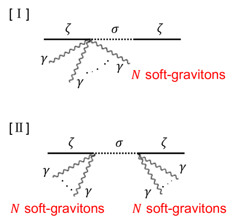
Figure 9: [I] ‘$(N,0)$ soft-gravitons’ diagram  and [II] ‘$(N,N)$ soft-gravitons’ diagram

5.1 General Considerations

[I] Computation of the ‘$(N,0)$ soft-gravitons’ diagram

The strategy for the computation of the ‘$(N,0)$ soft-graviton diagram’ is the same as in (3.11), and the calculation goes as follows:

$$\begin{split}&\langle\gamma^{s_{1}}(\mbox{\boldmath$q$}_{1})\cdots\gamma^{s_{N}}(\mbox{\boldmath$q$}_{N})\zeta(\mbox{\boldmath$k$}_{1})\zeta(\mbox{\boldmath$k$}_{2})\rangle\Big{|}_{{\rm Fig}.\>\ref{General}\>[{\rm I}]}\\ &=(2\pi)^{3}\delta^{3}(\mbox{\boldmath$q$}_{1}+\cdots+\mbox{\boldmath$q$}_{N}+\mbox{\boldmath$k$}_{1}+\mbox{\boldmath$k$}_{2})\\ &\qquad\times\epsilon_{ij}^{s_{1}}(\mbox{\boldmath$q$}_{1})\cdots\epsilon_{\alpha\beta}^{s_{N}}(\mbox{\boldmath$q$}_{N})(-i)^{2}\cdots(-i)^{2}(k_{2})_{i}(k_{2})_{j}\cdots(k_{2})_{\alpha}(k_{2})_{\beta}\\ &\qquad\times(-1)^{N}4\frac{C_{0}C_{N}}{H^{2}}\frac{H^{2}}{q_{1}^{3}}\cdots\frac{H^{2}}{q_{N}^{3}}\left(-\frac{H^{3}}{4\epsilon k_{1}}\right)\left(-\frac{H^{3}}{4\epsilon k_{2}}\right)\\ &\qquad\times e^{-\pi\textrm{Im}(\nu)}\frac{\pi}{4}H^{2}\,\times\,2!\times N!\\ &\times\Biggl{[}2\textrm{Re}\left[\int_{-\infty}^{0}\frac{d\eta_{1}}{\eta_{1}^{4}H^{4}}\int_{-\infty}^{0}\frac{d\eta_{2}}{(\eta_{2}H)^{4-2N}}\eta_{1}^{2}e^{-ik_{1}\eta_{1}}\eta_{2}^{2}e^{ik_{2}\eta_{2}}(\eta_{1}\eta_{2})^{\frac{3}{2}}H_{\nu}^{(1)}(-k_{2}\eta_{1})H_{\nu}^{(1)*}(-k_{2}\eta_{2})\right]\\ &\quad-2\textrm{Re}\left[\int_{-\infty}^{0}\frac{d\eta_{1}}{\eta_{1}^{4}H^{4}}\int_{-\infty}^{\eta_{1}}\frac{d\eta_{2}}{(\eta_{2}H)^{4-2N}}\eta_{1}^{2}e^{ik_{1}\eta_{1}}\eta_{2}^{2}e^{ik_{2}\eta_{2}}(\eta_{1}\eta_{2})^{\frac{3}{2}}H_{\nu}^{(1)}(-k_{2}\eta_{1})H_{\nu}^{(1)*}(-k_{2}\eta_{2})\right]\\ &\quad-2\textrm{Re}\left[\int_{-\infty}^{0}\frac{d\eta_{1}}{(\eta_{1}H)^{4-2N}}\int_{-\infty}^{\eta_{1}}\frac{d\eta_{2}}{\eta_{2}^{4}H^{4}}\eta_{1}^{2}e^{ik_{1}\eta_{1}}\eta_{2}^{2}e^{ik_{2}\eta_{2}}(\eta_{1}\eta_{2})^{\frac{3}{2}}H_{\nu}^{(1)}(-k_{2}\eta_{1})H_{\nu}^{(1)*}(-k_{2}\eta_{2})\right]\Biggl{]}.\end{split}$$ (5.5)

The factor $2!\times N!$ in the fifth line is a combinatorial factor for the diagram [I] in Figure 9. We then set $x\equiv-k_{2}\eta_{1}$ and $y\equiv-k_{2}\eta_{2}$ to find

$$\begin{split}&\langle\gamma^{s_{1}}(\mbox{\boldmath$q$}_{1})\cdots\gamma^{s_{N}}(\mbox{\boldmath$q$}_{N})\zeta(\mbox{\boldmath$k$}_{1})\zeta(\mbox{\boldmath$k$}_{2})\rangle\Big{|}_{{\rm Fig}.\>\ref{General}\>[{\rm I}]}\\ &=(2\pi)^{3}\delta^{3}(\mbox{\boldmath$q$}_{1}+\cdots+\mbox{\boldmath$q$}_{N}+\mbox{\boldmath$k$}_{1}+\mbox{\boldmath$k$}_{2})\\ &\qquad\times\epsilon_{ij}^{s_{1}}(\mbox{\boldmath$q$}_{1})\cdots\epsilon_{\alpha\beta}^{s_{N}}(\mbox{\boldmath$q$}_{N})\frac{(k_{2})_{i}(k_{2})_{j}}{(k_{2})^{2}}\cdots\frac{(k_{2})_{\alpha}(k_{2})_{\beta}}{(k_{2})^{2}}\\ &\qquad\times P_{\gamma}(q_{1})\cdots P_{\gamma}(q_{N})\ P_{\zeta}(k_{2})\frac{\pi C_{0}C_{N}}{\epsilon H^{4-2N}}N!\,e^{-\pi\textrm{Im}(\nu)}\\ &\qquad\times\Biggl{[}\textrm{Re}\left[\int_{0}^{\infty}dx\,x^{-\frac{1}{2}}e^{ix}H_{\nu}^{(1)}(x)\int_{0}^{\infty}dy\,y^{2N-\frac{1}{2}}e^{-iy}H_{\nu}^{(1)*}(y)\right]\\ &\qquad\quad-\textrm{Re}\left[\int_{0}^{\infty}dx\,x^{-\frac{1}{2}}e^{-ix}H_{\nu}^{(1)}(x)\int_{x}^{\infty}dy\,y^{2N-\frac{1}{2}}e^{-iy}H_{\nu}^{(1)*}(y)\right]\\ &\qquad\quad-\textrm{Re}\left[\int_{0}^{\infty}dx\,x^{2N-\frac{1}{2}}e^{-ix}H_{\nu}^{(1)}(x)\int_{x}^{\infty}dy\,y^{-\frac{1}{2}}e^{-iy}H_{\nu}^{(1)*}(y)\right]\Biggl{]}.\end{split}$$ (5.6)

We can compute these integrals just by using the formulae (A.6) and (B.16) in Appendices A and B and we obtain finally

$$\begin{split}\langle\gamma^{s_{1}}(\mbox{\boldmath$q$}_{1})&\cdots\gamma^{s_{N}}(\mbox{\boldmath$q$}_{N})\zeta(\mbox{\boldmath$k$}_{1})\zeta(\mbox{\boldmath$k$}_{2})\rangle\Big{|}_{{\rm Fig}.\>\ref{General}\>[{\rm I}]}\\ &=(2\pi)^{3}\delta^{3}(\mbox{\boldmath$q$}_{1}+\cdots+\mbox{\boldmath$q$}_{N}+\mbox{\boldmath$k$}_{1}+\mbox{\boldmath$k$}_{2})\\ &\qquad\times\epsilon_{ij}^{s_{1}}(\mbox{\boldmath$q$}_{1})\cdots\epsilon_{\alpha\beta}^{s_{N}}(\mbox{\boldmath$q$}_{N})\frac{(k_{2})_{i}(k_{2})_{j}}{(k_{2})^{2}}\cdots\frac{(k_{2})_{\alpha}(k_{2})_{\beta}}{(k_{2})^{2}}\\ &\qquad\times P_{\gamma}(q_{1})\cdots P_{\gamma}(q_{N})\ P_{\zeta}(k_{2})\frac{C_{0}C_{N}}{\epsilon H^{4-2N}}\,R_{N}(m),\end{split}$$ (5.7)

where we have introduced a function

$$\begin{split}&R_{N}(m)\equiv\\ &\,2^{1-2N}(-1)^{N}N!\\ &\times\Biggl{[}\frac{\pi^{2}}{\textrm{cosh}^{2}(\pi\mu)}\frac{1}{(2N)!}\left\{\left(2N-\frac{1}{2}\right)^{2}+\mu^{2}\right\}\cdots\left\{\left(\frac{3}{2}\right)^{2}+\mu^{2}\right\}\left\{\left(\frac{1}{2}\right)^{2}+\mu^{2}\right\}\\ &\quad-\frac{1}{\textrm{sinh}(\pi\mu)}\,\textrm{Re}\Biggl{[}\,\sum_{n=0}^{\infty}(-1)^{n}(n+1)(n+2)\cdots(n+2N)\\ &\qquad\times\Biggl{\{}e^{\pi\mu}\frac{(1+n+2i\mu)(2+n+2i\mu)\cdots(2N+n+2i\mu)\times(N+\frac{1}{2}+n+i\mu)}{(\frac{1}{2}+n+i\mu)^{2}(\frac{3}{2}+n+i\mu)\cdots(2N-\frac{1}{2}+n+i\mu)(2N+\frac{1}{2}+n+i\mu)^{2}}\\ &\qquad-e^{-\pi\mu}\frac{(1+n-2i\mu)(2+n-2i\mu)\cdots(2N+n-2i\mu)\times(N+\frac{1}{2}+n-i\mu)}{(\frac{1}{2}+n-i\mu)^{2}(\frac{3}{2}+n-i\mu)\cdots(2N-\frac{1}{2}+n-i\mu)(2N+\frac{1}{2}+n-i\mu)^{2}}\Biggl{\}}\Biggl{]}\Biggl{]}.\end{split}$$ (5.8)

This result is consistent with (3.15) for the $N=1$ case. Actually we can confirm that the function $R_{1}(m)$ coincides with $F_{2}(m)$ of (3.15).

[II] Computation of the ‘$(N,N)$ soft-gravitons’ diagram

This computation of the ‘$(N,N)$ soft-gravitons’ diagram goes along the same line as for (3.17) and we get

$$\begin{split}&\langle\gamma^{s_{1}}(\mbox{\boldmath$q$}_{1})\cdots\gamma^{s_{2N}}(\mbox{\boldmath$q$}_{2N})\zeta(\mbox{\boldmath$k$}_{1})\zeta(\mbox{\boldmath$k$}_{2})\rangle\Big{|}_{{\rm Fig}.\>\ref{General}\>[{\rm II}]}\\ &=(2\pi)^{3}\delta^{3}(\mbox{\boldmath$q$}_{1}+\cdots+\mbox{\boldmath$q$}_{2N}+\mbox{\boldmath$k$}_{1}+\mbox{\boldmath$k$}_{2})\\ &\qquad\times\epsilon_{ij}^{s_{1}}(\mbox{\boldmath$q$}_{1})\cdots\epsilon_{\alpha\beta}^{s_{2N}}(\mbox{\boldmath$q$}_{2N})(-i)^{2}\cdots(-i)^{2}(k_{2})_{i}(k_{2})_{j}\cdots(k_{2})_{\alpha}(k_{2})_{\beta}\\ &\qquad\times 4\frac{C_{N}^{2}}{H^{2}}\frac{H^{2}}{q_{1}^{3}}\cdots\frac{H^{2}}{q_{2N}^{3}}\left(-\frac{H^{3}}{4\epsilon k_{1}}\right)\left(-\frac{H^{3}}{4\epsilon k_{2}}\right)\\ &\qquad\times e^{-\pi\textrm{Im}(\nu)}\frac{\pi}{4}H^{2}\,\times\,2!\times(2N)!\\ &\times\Biggl{[}\int_{-\infty}^{0}\frac{d\eta_{1}}{(\eta_{1}H)^{4-2N}}\int_{-\infty}^{0}\frac{d\eta_{2}}{(\eta_{2}H)^{4-2N}}\eta_{1}^{2}e^{-ik_{1}\eta_{1}}\eta_{2}^{2}e^{ik_{2}\eta_{2}}(\eta_{1}\eta_{2})^{\frac{3}{2}}H_{\nu}^{(1)}(-k_{2}\eta_{1})H_{\nu}^{(1)*}(-k_{2}\eta_{2})\\ &-2\textrm{Re}\left[\int_{-\infty}^{0}\frac{d\eta_{1}}{(\eta_{1}H)^{4-2N}}\int_{-\infty}^{\eta_{1}}\frac{d\eta_{2}}{(\eta_{2}H)^{4-2N}}\eta_{1}^{2}e^{ik_{1}\eta_{1}}\eta_{2}^{2}e^{ik_{2}\eta_{2}}(\eta_{1}\eta_{2})^{\frac{3}{2}}H_{\nu}^{(1)}(-k_{2}\eta_{1})H_{\nu}^{(1)*}(-k_{2}\eta_{2})\right]\Biggl{]}.\end{split}$$ (5.9)

As before, the factor $2!\times(2N)!$ in the fifth line is a combinatorial factor for the diagram [II] in Figure 9. By setting $x\equiv-k_{2}\eta_{1}$ and $y\equiv-k_{2}\eta_{2}$, we can put (5.9) into the following form,

$$\begin{split}&\langle\gamma^{s_{1}}(\mbox{\boldmath$q$}_{1})\cdots\gamma^{s_{2N}}(\mbox{\boldmath$q$}_{2N})\zeta(\mbox{\boldmath$k$}_{1})\zeta(\mbox{\boldmath$k$}_{2})\rangle\Big{|}_{{\rm Fig}.\>\ref{General}\>[{\rm II}]}\\ &=(2\pi)^{3}\delta^{3}(\mbox{\boldmath$q$}_{1}+\cdots+\mbox{\boldmath$q$}_{2N}+\mbox{\boldmath$k$}_{1}+\mbox{\boldmath$k$}_{2})\\ &\qquad\times\epsilon_{ij}^{s_{1}}(\mbox{\boldmath$q$}_{1})\cdots\epsilon_{\alpha\beta}^{s_{2N}}(\mbox{\boldmath$q$}_{2N})\frac{(k_{2})_{i}(k_{2})_{j}}{(k_{2})^{2}}\cdots\frac{(k_{2})_{\alpha}(k_{2})_{\beta}}{(k_{2})^{2}}\\ &\qquad\times P_{\gamma}(q_{1})\cdots P_{\gamma}(q_{2N})\ P_{\zeta}(k_{2})\frac{\pi C_{N}^{2}}{\epsilon H^{4(1-N)}}(2N)!\,e^{-\pi\textrm{Im}(\nu)}\\ &\qquad\times\Biggl{[}\frac{1}{2}\left|\int_{0}^{\infty}dx\,x^{2N-\frac{1}{2}}e^{ix}H_{\nu}^{(1)}(x)\right|^{2}\\ &\qquad\quad-\textrm{Re}\left[\int_{0}^{\infty}dx\,x^{2N-\frac{1}{2}}e^{-ix}H_{\nu}^{(1)}(x)\int_{x}^{\infty}dy\,y^{2N-\frac{1}{2}}e^{-iy}H_{\nu}^{(1)*}(y)\right]\Biggl{]}.\end{split}$$ (5.10)

Finally we make use of the integration formulae (A.6) and (B.16) in Appendices A and B and this correlation function turns out to be

$$\begin{split}\langle\gamma^{s_{1}}(\mbox{\boldmath$q$}_{1})&\cdots\gamma^{s_{2N}}(\mbox{\boldmath$q$}_{2N})\zeta(\mbox{\boldmath$k$}_{1})\zeta(\mbox{\boldmath$k$}_{2})\rangle\Big{|}_{{\rm Fig}.\>\ref{General}\>[{\rm II}]}\\ &=(2\pi)^{3}\delta^{3}(\mbox{\boldmath$q$}_{1}+\cdots+\mbox{\boldmath$q$}_{2N}+\mbox{\boldmath$k$}_{1}+\mbox{\boldmath$k$}_{2})\\ &\qquad\times\epsilon_{ij}^{s_{1}}(\mbox{\boldmath$q$}_{1})\cdots\epsilon_{\alpha\beta}^{s_{2N}}(\mbox{\boldmath$q$}_{2N})\frac{(k_{2})_{i}(k_{2})_{j}}{(k_{2})^{2}}\cdots\frac{(k_{2})_{\alpha}(k_{2})_{\beta}}{(k_{2})^{2}}\\ &\qquad\times P_{\gamma}(q_{1})\cdots P_{\gamma}(q_{2N})\ P_{\zeta}(k_{2})\frac{C_{N}^{2}}{\epsilon H^{4(1-N)}}\,S_{N}(m),\end{split}$$ (5.11)

where we have defined a function

$$\begin{split}&S_{N}(m)\equiv\\ &2^{-4N}\Biggl{[}\frac{\pi^{2}}{\textrm{cosh}^{2}(\pi\mu)}\frac{1}{(2N)!}\left\{\left(2N-\frac{1}{2}\right)^{2}+\mu^{2}\right\}^{2}\cdots\left\{\left(\frac{3}{2}\right)^{2}+\mu^{2}\right\}^{2}\left\{\left(\frac{1}{2}\right)^{2}+\mu^{2}\right\}^{2}\\ &\quad-\frac{(2N)!}{\textrm{sinh}(\pi\mu)}\,\textrm{Re}\Biggl{[}\,\sum_{n=0}^{\infty}(-1)^{n}(n+1)(n+2)\cdots(n+4N)\\ &\qquad\times\Biggl{\{}e^{\pi\mu}\frac{(1+n+2i\mu)(2+n+2i\mu)\cdots(4N+n+2i\mu)}{(\frac{1}{2}+n+i\mu)(\frac{3}{2}+n+i\mu)\cdots(2N+\frac{1}{2}+n+i\mu)^{2}\cdots(4N+\frac{1}{2}+n+i\mu)}\\ &\qquad-e^{-\pi\mu}\frac{(1+n-2i\mu)(2+n-2i\mu)\cdots(4N+n-2i\mu)}{(\frac{1}{2}+n-i\mu)(\frac{3}{2}+n-i\mu)\cdots(2N+\frac{1}{2}+n-i\mu)^{2}\cdots(4N+\frac{1}{2}+n-i\mu)}\Biggl{\}}\Biggl{]}\Biggl{]}.\end{split}$$ (5.12)

This result is consistent with (3.20) for the $N=1$ case. In fact we can confirm that the function $S_{1}(m)$ coincides with $F_{3}(m)$ of (3.20).

5.2 Evaluation of the functions $R_{N}(m)$ and $S_{N}(m)$

To have an insight into the sensitivity of the correlation $\langle\gamma^{s_{1}}\cdots\gamma^{s_{N}}\zeta\zeta\rangle$ to the mass $m$, let us consider the functions $R_{N}(m)$ for $N=1,2,3$ and $4$, whose $m$-dependence are illustrated in Figure 10. As we can see easily in Figure 10 , the peak of the correlation function is shifted to larger values of the mass $m$ of $\sigma$ as the number of the soft-gravitons increases.

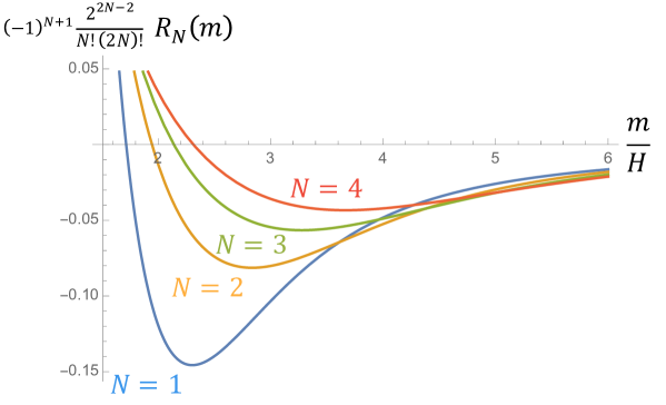
Figure 10: The plots for $(-1)^{N+1}\frac{2^{2N-2}}{N!(2N)!}R_{N}(m)$ when $N=1,2,3$ and $4$ in $m\geq 1.5H$. The factor $(-1)^{N+1}\frac{2^{2N-2}}{N!(2N)!}$ is introduced for the functions to converge to the same value when $m\to\infty$; we will discuss this in the subsection 5.3, and this factor is shown in (5.17).

Similarly we also plot the behavior of the function of $S_{N}(m)$ for $N=1$ and $2$ in Figure 11. Although we were able to study only two cases $N=1$ and $N=2$, because of the limited computational power, it is likely that the positions of the peaks are shifted to larger values of the mass $m$ of $\sigma$ as $N$ becomes large. We may safely say that correlation functions involving larger number of gravitons would be useful for probing larger values of $m$.

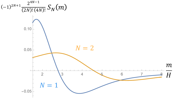
Figure 11: The plots for $(-1)^{2N+1}\frac{2^{4N-1}}{(2N)!(4N)!}S_{N}(m)$ when $N=1$ and $2$ in $m\geq 1.5H$. The factor $(-1)^{2N+1}\frac{2^{4N-1}}{(2N)!(4N)!}$ is introduced for the same reason as Figure 10, and it is shown in (5.18).

We are able to see from Figures 10 and 11 that the functions $R_{N}(m)$ and $S_{N}(m)$ both go down quickly for large $m$, and that the speed of the decrease seems to be shared among them. As one may surmise from (5.8) and (5.12), a numerical check of the speed of their decrease is not easy to do for large $N$. Therefore, here we examine only the ratios of $R_{1}(m)$, $R_{2}(m)$, $R_{3}(m)$ and $S_{1}(m)$ for $m\gg H$ and some of the results are listed in Tables 2 and 3. We can safely conclude from the numbers listed in Table 2 that the limiting behavior is $R_{2}(m)/R_{1}(m)\to-6$ and $R_{2}(m)/S_{1}(m)\to 2$ as $m/H\to\infty$. In the next subsection we will develop a method to explain these limits, thereby the limiting value suggested in Table 3 will also be explained.

Table 2: The numerical analysis of $R_{2}(m)/R_{1}(m)$ and $R_{2}(m)/S_{1}(m)$

$\displaystyle m/H$	$\displaystyle 5.0$	$\displaystyle 10.0$	$\displaystyle 15.0$	$\displaystyle 20.0$	$\displaystyle 25.0$	$\displaystyle 30.0$
$\displaystyle R_{2}(m)/R_{1}(m)$	$\displaystyle-6.88167$	$\displaystyle-6.14334$	$\displaystyle-6.05725$	$\displaystyle-6.03114$	$\displaystyle-6.02061$	$\displaystyle-6.01494$
$\displaystyle R_{2}(m)/S_{1}(m)$	$\displaystyle 1.61009$	$\displaystyle 1.90731$	$\displaystyle 1.96234$	$\displaystyle 1.97926$	$\displaystyle 1.98754$	$\displaystyle 1.99115$

Table 3: The numerical analysis of $R_{3}(m)/R_{2}(m)$

$\displaystyle m/H$	$\displaystyle 5.0$	$\displaystyle 7.0$	$\displaystyle 9.0$	$\displaystyle 11.0$	$\displaystyle 13.0$	$\displaystyle 15.0$
$\displaystyle R_{3}(m)/R_{2}(m)$	$\displaystyle-24.137$	$\displaystyle-24.242$	$\displaystyle-23.3081$	$\displaystyle-22.9589$	$\displaystyle-22.7956$	$\displaystyle-22.7469$

5.3 The large mass behavior

The strategy to study the asymptotic behaviors of $R_{N}(m)$ and $S_{N}(m)$ for large $m$ is almost the same as in Section 4. We suppose that the dynamical degrees of freedom of $\sigma$ are integrated out in Figure 9 and we introduce effective interaction Hamiltonian as illustrated in Figure 12. Starting from the interaction Hamiltonian (5.4), we are able to read off effective interactions corresponding to diagrams on the right hand side in Figure 12. Namely we get

$$H_{I}(t)\Bigg{|}_{{\rm Fig.}\ref{simplifiedgene}\>[{\rm I}]}=(-1)^{N}4\frac{C_{0}C_{N}}{H^{2}}a^{3-2N}(t)f(m)\int d^{3}x\ \dot{\zeta}\gamma_{ij}\cdots\gamma_{\alpha\beta}\partial_{i}\partial_{j}\cdots\partial_{\alpha}\partial_{\beta}\dot{\zeta}\ \times 2,$$ (5.13)

$$\begin{split}H_{I}(t)\Bigg{|}_{{\rm Fig.}\ref{simplifiedgene}\>[{\rm II}]}=4\frac{C_{N}^{2}}{H^{2}}a^{3-4N}(t)f(m)\int d^{3}x\ \gamma_{ij}&\cdots\gamma_{\alpha\beta}\partial_{i}\partial_{j}\cdots\partial_{\alpha}\partial_{\beta}\dot{\zeta}\\ &\times\gamma_{i^{\prime}j^{\prime}}\cdots\gamma_{\alpha^{\prime}\beta^{\prime}}\partial_{i^{\prime}}\partial_{j^{\prime}}\cdots\partial_{\alpha^{\prime}}\partial_{\beta^{\prime}}\dot{\zeta}.\end{split}$$ (5.14)

for [I] and [II] in Figure 12, respectively. Note that the function $f(m)$, whose explicit form is not specified here, is common both in (5.13) and (5.14).

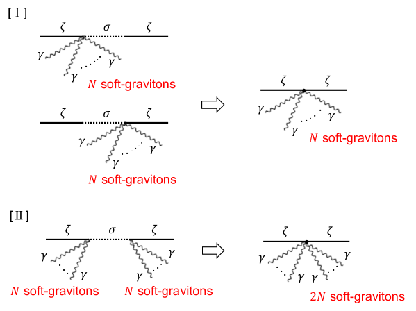
Figure 12: The simplified diagrams when $m\to\infty$

Once we have the effective interactions (5.13) and (5.14), it is almost straightforward to work out the correlation functions, which turn out to be

$$\begin{split}\langle\gamma^{s_{1}}(\mbox{\boldmath$q$}_{1})\cdots&\gamma^{s_{N}}(\mbox{\boldmath$q$}_{N})\zeta(\mbox{\boldmath$k$}_{1})\zeta(\mbox{\boldmath$k$}_{2})\rangle\bigg{|}_{{\rm Fig.}\>\ref{simplifiedgene}\>[{\rm I}]}\\ &=(2\pi)^{3}\delta^{3}(\mbox{\boldmath$q$}_{1}+\cdots+\mbox{\boldmath$q$}_{N}+\mbox{\boldmath$k$}_{1}+\mbox{\boldmath$k$}_{2})\\ &\qquad\times\epsilon_{ij}^{s_{1}}(\mbox{\boldmath$q$}_{1})\cdots\epsilon_{\alpha\beta}^{s_{N}}(\mbox{\boldmath$q$}_{N})(-i)^{2}\cdots(-i)^{2}(k_{2})_{i}(k_{2})_{j}\cdots(k_{2})_{\alpha}(k_{2})_{\beta}\\ &\qquad\times f(m)(-1)^{N}4\frac{C_{0}C_{N}}{H^{2}}\frac{H^{2}}{q_{1}^{3}}\cdots\frac{H^{2}}{q_{N}^{3}}\left(-\frac{H^{3}}{4\epsilon k_{1}}\right)\left(-\frac{H^{3}}{4\epsilon k_{2}}\right)\times 2\\ &\qquad\quad\times\,2!\times N!\\ &\qquad\quad\times 2\,\textrm{Im}\left[\int_{-\infty}^{0}\frac{d\eta}{(\eta H)^{4-2N}}\eta^{2}e^{ik_{1}\eta}\eta^{2}e^{ik_{2}\eta}\right]\end{split}$$

$$\begin{split}&=(2\pi)^{3}\delta^{3}(\mbox{\boldmath$q$}_{1}+\cdots+\mbox{\boldmath$q$}_{N}+\mbox{\boldmath$k$}_{1}+\mbox{\boldmath$k$}_{2})\\ &\qquad\times\epsilon_{ij}^{s_{1}}(\mbox{\boldmath$q$}_{1})\cdots\epsilon_{\alpha\beta}^{s_{N}}(\mbox{\boldmath$q$}_{N})\frac{(k_{2})_{i}(k_{2})_{j}}{(k_{2})^{2}}\cdots\frac{(k_{2})_{\alpha}(k_{2})_{\beta}}{(k_{2})^{2}}\\ &\qquad\times P_{\gamma}(q_{1})\cdots P_{\gamma}(q_{N})\ P_{\zeta}(k_{2})\frac{C_{0}C_{N}}{\epsilon H^{4-2N}}\,\tilde{R}_{N}(m),\end{split}$$ (5.15)

$$\begin{split}\langle\gamma^{s_{1}}(\mbox{\boldmath$q$}_{1})\cdots&\gamma^{s_{2N}}(\mbox{\boldmath$q$}_{2N})\zeta(\mbox{\boldmath$k$}_{1})\zeta(\mbox{\boldmath$k$}_{2})\rangle\bigg{|}_{{\rm Fig.}\>\ref{simplifiedgene}\>[{\rm II}]}\\ &=(2\pi)^{3}\delta^{3}(\mbox{\boldmath$q$}_{1}+\cdots+\mbox{\boldmath$q$}_{2N}+\mbox{\boldmath$k$}_{1}+\mbox{\boldmath$k$}_{2})\\ &\qquad\times\epsilon_{ij}^{s_{1}}(\mbox{\boldmath$q$}_{1})\cdots\epsilon_{\alpha\beta}^{s_{2N}}(\mbox{\boldmath$q$}_{2N})(-i)^{2}\cdots(-i)^{2}(k_{2})_{i}(k_{2})_{j}\cdots(k_{2})_{\alpha}(k_{2})_{\beta}\\ &\qquad\times f(m)\,4\frac{C_{N}^{2}}{H^{2}}\frac{H^{2}}{q_{1}^{3}}\cdots\frac{H^{2}}{q_{N}^{3}}\left(-\frac{H^{3}}{4\epsilon k_{1}}\right)\left(-\frac{H^{3}}{4\epsilon k_{2}}\right)\,\times\,2!\times(2N)!\\ &\qquad\times 2\,\textrm{Im}\left[\int_{-\infty}^{0}\frac{d\eta}{(\eta H)^{4(1-N)}}\eta^{2}e^{ik_{1}\eta}\eta^{2}e^{ik_{2}\eta}\right]\end{split}$$

$$\begin{split}&=(2\pi)^{3}\delta^{3}(\mbox{\boldmath$q$}_{1}+\cdots+\mbox{\boldmath$q$}_{2N}+\mbox{\boldmath$k$}_{1}+\mbox{\boldmath$k$}_{2})\\ &\qquad\times\epsilon_{ij}^{s_{1}}(\mbox{\boldmath$q$}_{1})\cdots\epsilon_{\alpha\beta}^{s_{2N}}(\mbox{\boldmath$q$}_{2N})\frac{(k_{2})_{i}(k_{2})_{j}}{(k_{2})^{2}}\cdots\frac{(k_{2})_{\alpha}(k_{2})_{\beta}}{(k_{2})^{2}}\\ &\qquad\times P_{\gamma}(q_{1})\cdots P_{\gamma}(q_{2N})\ P_{\zeta}(k_{2})\frac{C_{N}^{2}}{\epsilon H^{4(1-N)}}\,\tilde{S}_{N}(m).\end{split}$$ (5.16)

Here we have introduced two notations

$$\tilde{R}_{N}(m)\equiv H^{2}f(m)\times(-1)^{N+1}\frac{N!(2N)!}{2^{2N-2}}\>,$$ (5.17)

$$\tilde{S}_{N}(m)\equiv H^{2}f(m)\times(-1)^{2N+1}\frac{(2N)!(4N)!}{2^{4N-1}}\>.$$ (5.18)

Comparison of these results with (5.7) and (5.11) tells us immediately that $\tilde{R}_{N}(m)$ and $\tilde{S}_{N}(m)$ correspond respectively to $R_{N}(m)$ and $S_{N}(m)$ in the $m\to\infty$ limit. Using (5.17) and (5.18), we can find the relations:

$$\frac{\tilde{R}_{N+1}(m)}{\tilde{R}_{N}(m)} = -\frac{(N+1)^{2}(2N+1)}{2},$$ (5.19)

$$\frac{\tilde{R}_{2N}(m)}{\tilde{S}_{N}(m)} = 2.$$ (5.20)

Note that the relation (5.20) is trivial because this ‘2’ is produced by the fact that there are two original diagrams in [I] of Figure 12. On the other hand, the relation (5.19) is important in the sense that it serves as a consistency relation relating $\langle\gamma^{s_{1}}\cdots\gamma^{s_{N+1}}\zeta\zeta\rangle$ to $\langle\gamma^{s_{1}}\cdots\gamma^{s_{N}}\zeta\zeta\rangle$ in the $m\to\infty$ limit in this model. This relation could be useful when searching for new particles whose masses are much greater than $10^{14}$ GeV.

Finally we would like to check the numerical analysis done before. When $N=1$, (5.19) and (5.20) become

$$\frac{\tilde{R}_{2}(m)}{\tilde{R}_{1}(m)}=-6,\quad\frac{\tilde{R}_{2}(m)}{\tilde{S}_{1}(m)}=2,$$ (5.21)

which are consistent with Table 2. Note that as a consequence of (5.21) we get $\tilde{R}_{1}(m)/\tilde{S}_{1}(m)=-1/3$ which is nothing but the relation (4.12). If we put $N=2$ in (5.19), it becomes

$$\frac{\tilde{R}_{3}(m)}{\tilde{R}_{2}(m)}=-\frac{45}{2}.$$ (5.22)

This is also consistent with Table 3.

6 Summary

In the present paper we have searched for the possibility that the cosmological data could be useful to get hold of unknown heavy particles whose masses are on the order of the Hubble parameter $H$ during inflation. To be more specific we considered the quasi-single field inflation model [10] and tried to develop the methodology of getting signatures of the isocurvaton $\sigma$ in the CMB data. In contrast with previous similar attempts [11], we have paid more attention to correlation functions containing tensor perturbation $\gamma$ than those of scalar perturbation $\zeta$ only. To keep our investigation as general as possible, we made use of the EFT technique for inflation [3, 4, 5].

The EFT method tells us that there would exist couplings of the type $\zeta\sigma$ and $\gamma\zeta\sigma$ and these couplings could produce potentially observable effects on the power spectrum of $\zeta$ and some of the correlation functions. We have therefore launched into detailed study of these effects on $\langle\zeta\zeta\rangle$, $\langle\gamma\zeta\zeta\rangle$ and $\langle\gamma\gamma\zeta\zeta\rangle$. Being particularly interested in their dependence on the mass of $\sigma$, we have derived concise formulae of these correlation functions in the form amenable to numerical analyses as given in (3.7), (3.14) and (3.19). The $m$-dependences of the correlation functions are illustrated in Figures 4, 5 and 6. The effects due to $\sigma$ to these correlation functions go down to zero quickly as $m\to\infty$, but we have noticed that the large $m$ behavior of these effects has some common nature. We gave a simple explanation of the asymptotic behavior by introducing a short-cut method as illustrated in Figure 8. If we could measure the correlation functions $\langle\gamma\zeta\zeta\rangle$ and $\langle\gamma\gamma\zeta\zeta\rangle$, precise enough in future observation, then we could determine the strength of couplings $\zeta\sigma$ and $\gamma\zeta\sigma$ together with the mass $m$ .

We then went one step further to generalize the above consideration to an aribitrary number of gravitons. Namely by exploiting the EFT method we constructed a coupling of $\zeta$, $\sigma$ and $N$-gravitons, and computed $\langle\gamma^{s_{1}}\cdots\gamma^{s_{N}}\zeta\zeta\rangle$ and $\langle\gamma^{s_{1}}\cdots\cdots\gamma^{s_{2N}}\zeta\zeta\rangle$ by using this coupling once and twice, respectively as shown in Figure 9. Formulae of these correlations are summarized in (5.7) and (5.11), and their $m$ dependence has been studied numerically. The asymptotic behaviors of the correlations for $m\to\infty$ were also studied by a short-cut method as in the $N=1$ case. From these analyses we have seen that the peaks of these correlations move to a larger value of $m$ as $N$ increases. Therefore multiple-graviton correlation functions are more appropriate tools to probe larger values of the mass $m$.

In the present paper we have taken up a particular model, i.e., the quasi-single field inflation model in order to make our analyses as definite as possible. In this case, therefore, the heavy particle is $\sigma$ and is necessarily spinless. From the standpoint of developing a technique to probe unknown heavy particles in the cosmological data, however, it is more desirable to be able to handle higher-spin particles as generally as possible. At present we do not have much to say about higher-spin case, but hopefully our present analyses could offer a clue for such an extension.

Appendix A The integration formulae (I)

We now perform the integration of the following type

$$\int_{0}^{\infty}dx\ x^{l}e^{ix}H_{i\mu}^{(1)}(x),$$ (A.1)

which appears in (3.5), (3.12) and (3.18)。 Note that $l$ is either $-1/2$ or $3/2$, and

$$\nu=i\mu=i\sqrt{\frac{m^{2}}{H^{2}}-\frac{9}{4}}\>.$$ (A.2)

From here, we assume that $\mu$ is real, which means $m\geq 3H/2$.

Firstly, we perform the indefinite integration by employing Mathematica 11:

$$\begin{split}\int&dx\ x^{l}e^{ix}H_{i\mu}^{(1)}(x)\\ &=x^{1+l-i\mu}\frac{-2^{i\mu}\textrm{csch}(\pi\mu)}{(1+l-i\mu)\Gamma(1-i\mu)}\,{}_{2}F_{2}(a_{1},a_{1}+\frac{1}{2}+l;2a_{1},a_{1}+\frac{3}{2}+l;z)\\ &+x^{1+l+i\mu}\frac{2^{-i\mu}(1+\textrm{coth}(\pi\mu))}{(1+l+i\mu)\Gamma(1+i\mu)}\,{}_{2}F_{2}(a_{2},a_{2}+\frac{1}{2}+l;2a_{2},a_{2}+\frac{3}{2}+l;z),\end{split}$$ (A.3)

where $a_{1}\equiv 1/2-i\mu$, $a_{2}\equiv 1/2+i\mu$ and $z\equiv 2ix$. Note that ${}_{p}F_{q}$ is the generalized hypergeometric function

$${}_{p}F_{q}(a_{1},\cdots,a_{p};b_{1},\cdots,b_{q};z)=\sum_{n=0}^{\infty}\frac{(a_{1})_{n}\cdots(a_{p})_{n}}{(b_{1})_{n}\cdots(b_{q})_{n}}\frac{z^{n}}{n!},$$ (A.4)

in which $(a)_{n}\equiv a(a+1)\cdots(a+n-1)$ for $n\geq 1$ and $(a)_{0}=1$, and that (A.3) vanishes when $x=0$. In Eq. (A.3) we used the notaion $\textrm{csch}(\pi\mu)=1/\textrm{sinh}(\pi\mu)$. In order to know the large $x$ behavior of (A.3) , we have to examine the asymptotic behavior of ${}_{2}F_{2}$. The leading terms can be obtained by Mathematica 11:

$$\begin{split}&\lim_{z\to\infty}{}_{2}F_{2}(a,a+\frac{1}{2}+l;2a,a+\frac{3}{2}+l;z)\\ &=z^{-\frac{1}{2}-a-l}(-1)^{\frac{3}{2}-a-l}2^{-2+2a}\frac{(1+2a+2l)}{\sqrt{\pi}}\frac{\Gamma(\frac{1}{2}+a)\Gamma(-\frac{1}{2}-l)\Gamma(\frac{1}{2}+a+l)}{\Gamma(-\frac{1}{2}+a-l)}\\ &\qquad+e^{z}z^{-1-a}(\cdots)+z^{-a}(\cdots).\end{split}$$ (A.5)

Here both of the ellipses $(\cdots)$ are functions of $a$ and $l$. The term $e^{z}z^{-1-a}(\cdots)$ can be eliminated using the $i\epsilon$ prescription. In addition, the terms $z^{-a_{1}}(\cdots)$ and $z^{-a_{2}}(\cdots)$ are canceled by each other in (A.3) . Therefore, we need to consider only the first term in (A.5). Substituting it into (A.3) and performing some calculations, we obtain the following result:

$$\int_{0}^{\infty}dx\ x^{l}e^{ix}H_{i\mu}^{(1)}(x)=e^{\frac{\pi\mu}{2}}\frac{(i/2)^{l}}{\sqrt{\pi}}\frac{\Gamma(1+l-i\mu)\Gamma(1+l+i\mu)}{\Gamma(l+\frac{3}{2})}.$$ (A.6)

For $l=-1/2$ and $l=3/2$, (A.6) turns out to be

$$\int_{0}^{\infty}dx\ x^{-\frac{1}{2}}e^{ix}H_{i\mu}^{(1)}(x)=\frac{\sqrt{\pi}\,e^{\frac{\pi\mu}{2}}}{\textrm{cosh}(\pi\mu)}(1-i)$$ (A.7)

and

$$\begin{split}\int_{0}^{\infty}dx&\ x^{\frac{3}{2}}e^{ix}H_{i\mu}^{(1)}(x)\\ &=\frac{\sqrt{\pi}\,e^{\frac{\pi\mu}{2}}}{\textrm{cosh}(\pi\mu)}(-1+i)\times\frac{1}{8}\left(\frac{1}{4}+\mu^{2}\right)\left(\frac{9}{4}+\mu^{2}\right),\end{split}$$ (A.8)

respectively.

Appendix B The integration formulae (II)

We now turn to the evaluation of the integral

$$\int_{0}^{\infty}dx\ x^{m}e^{-ix}H_{i\mu}^{(1)}(x)\int_{x}^{\infty}dy\ y^{l}e^{-iy}H_{i\mu}^{(1)*}(y).$$ (B.1)

which also appears in (3.5), (3.12) and (3.18). Note that $(l,m)$ is either $(-1/2,-1/2)$, $(3/2,-1/2)$, $(-1/2,3/2)$ or $(3/2,3/2)$, and $\nu$ is given by (A.2). As before we assume that $\mu$ is real, or equivalently $m\geq 3H/2$.

We use the ‘resummation’ trick [29]. Firstly, we rewrite (B.1) using the definition of the Hankel function as

$$\begin{split}\int_{0}^{\infty}dx\ &x^{m}e^{-ix}H_{i\mu}^{(1)}(x)\,\mathcal{I}(x)\\ &=\left[1+\textrm{coth}(\pi\mu)\right]\int_{0}^{\infty}dx\ x^{m}e^{-ix}J_{i\mu}(x)\,\mathcal{I}(x)\\ &\qquad-\textrm{csch}(\pi\mu)\int_{0}^{\infty}dx\ x^{m}e^{-ix}J_{-i\mu}(x)\,\mathcal{I}(x),\end{split}$$ (B.2)

where we have defined

$$\mathcal{I}(x)\equiv\int_{x}^{\infty}dy\ y^{l}e^{-iy}H_{i\mu}^{(1)*}(y).$$ (B.3)

Then, using the series expansions

$$J_{i\mu}(x)=\sum_{n=0}^{\infty}a_{2n}x^{2n},\qquad\quad a_{2n}=x^{i\mu}\,2^{-i\mu}\frac{(-1)^{n}\,2^{-2n}}{n!\,\Gamma(1+n+i\mu)},$$ (B.4)

$$e^{-ix}=\sum_{n=0}^{\infty}b_{n}x^{n},\qquad\quad b_{n}=\frac{(-i)^{n}}{n!},$$ (B.5)

we rewrite the integrand in (B.2) also in power series

$$x^{m}e^{-ix}J_{i\mu}(x) = \sum_{n=0}^{\infty}\left(\sum_{k=0}^{n}a_{2k}b_{n-2k}\right)x^{n+m}$$

$$= \sum_{n=0}^{\infty}\frac{(-i)^{n}\,2^{n+i\mu}\Gamma(\frac{1}{2}+n+i\mu)}{\sqrt{\pi}\,n!\,\Gamma(1+n+2i\mu)}x^{n+m+i\mu}$$

$$=: \sum_{n=0}^{\infty}\ c_{n}^{+}\ x^{n+m+i\mu}.$$

The coefficient $c_{n}^{+}$ is defined by the last equality. Note that the summation in the first line above is performed by Mathematica 11. Similarly, we are able to derive

$$x^{m}e^{-ix}J_{-i\mu}(x) = \sum_{n=0}^{\infty}\frac{(-i)^{n}\,2^{n-i\mu}\Gamma(\frac{1}{2}+n-i\mu)}{\sqrt{\pi}\,n!\,\Gamma(1+n-2i\mu)}x^{n+m-i\mu}$$

$$=: \sum_{n=0}^{\infty}\ c_{n}^{-}\ x^{n+m-i\mu}.$$

Here again $c_{n}^{-}$ is defined by the last equality. Substituting (B) and (B) into (B.2), we end up with

$$\begin{split}\int_{0}^{\infty}dx\ x^{m}e^{-ix}&H_{i\mu}^{(1)}(x)\,\mathcal{I}(x)\\ &=\left[1+\textrm{coth}(\pi\mu)\right]\sum_{n=0}^{\infty}c_{n}^{+}\int_{0}^{\infty}dx\ x^{n+m+i\mu}\ \mathcal{I}(x)\\ &\qquad-\textrm{csch}(\pi\mu)\sum_{n=0}^{\infty}c_{n}^{-}\int_{0}^{\infty}dx\ x^{n+m-i\mu}\ \mathcal{I}(x).\end{split}$$ (B.8)

Next, we evaluate the definite integral $\mathcal{I}(x)$ by taking the complex conjugate of the results in (A.6) and (A.3):

$$\begin{split}\mathcal{I}(x)&\equiv\int_{x}^{\infty}dy\ y^{l}e^{-iy}H_{i\mu}^{(1)*}(y)\\ &=e^{\frac{\pi\mu}{2}}\frac{(-i/2)^{l}}{\sqrt{\pi}}\frac{\Gamma(1+l+i\mu)\Gamma(1+l-i\mu)}{\Gamma(l+\frac{3}{2})}\\ &\quad+x^{1+l+i\mu}\frac{2^{-i\mu}\,\textrm{csch}(\pi\mu)}{(1+l+i\mu)\Gamma(1+i\mu)}\,{}_{2}F_{2}(a_{2},a_{2}+\frac{1}{2}+l;2a_{2},a_{2}+\frac{3}{2}+l;-2ix)\\ &\quad-x^{1+l-i\mu}\frac{2^{i\mu}(1+\textrm{coth}(\pi\mu))}{(1+l-i\mu)\Gamma(1-i\mu)}\,{}_{2}F_{2}(a_{1},a_{1}+\frac{1}{2}+l;2a_{1},a_{1}+\frac{3}{2}+l;-2ix).\end{split}$$ (B.9)

Using the expression (B.9), the integration over $x$ gives us formally the following

$$\begin{split}\int_{0}^{\infty}&dx\ x^{n+m+i\mu}\ \mathcal{I}(x)\\ &=e^{\frac{\pi\mu}{2}}\frac{(-i/2)^{l}}{\sqrt{\pi}}\frac{\Gamma(1+l+i\mu)\Gamma(1+l-i\mu)}{\Gamma(l+\frac{3}{2})}\left.\frac{x^{1+m+n+i\mu}}{1+m+n+i\mu}\right|_{x\to\infty}\\ &\quad+\frac{2^{-i\mu}\,\textrm{csch}(\pi\mu)}{(1+l+i\mu)\Gamma(1+i\mu)}\int_{0}^{\infty}dx\ x^{1+l+m+n+2i\mu}{}_{2}F_{2}(a_{2},\cdots;-2ix)\\ &\quad-\frac{2^{i\mu}(1+\textrm{coth}(\pi\mu))}{(1+l-i\mu)\Gamma(1-i\mu)}\int_{0}^{\infty}dx\ x^{1+l+m+n}{}_{2}F_{2}(a_{1},\cdots;-2ix).\end{split}$$ (B.10)

The first term on the right hand side of (B.10) is divergent, but this term is actually cancelled by the remaining terms. In order to confirm this, we have to evaluate the integrals in (B.10).

The indefinite integral is known to be

$$\begin{split}\int dx\ &x^{p+n}{}_{2}F_{2}(a,a+\frac{1}{2}+l;2a,a+\frac{3}{2}+l;-2ix)\\ &=\frac{(1+2a+2l)\,x^{1+p+n}\,{}_{2}F_{2}(a,1+p+n;2a,2+p+n;-2ix)}{(1+p+n)(-1+2a-2p+2l-2n)}\\ &\quad+\frac{2x^{1+p+n}\,{}_{2}F_{2}(a,a+\frac{1}{2}+l;2a,a+\frac{3}{2}+l;-2ix)}{1-2a+2p-2l+2n},\end{split}$$ (B.11)

where $p$ is set $p\equiv 1+l+m+2i\mu$ for the second term in (B.10) while $p\equiv 1+l+m$ for the third term in (B.10). Note that when $x=0$, the right hand side of (B.11) vanishes. When $x\to\infty$ on the other hand, we have to know the asymptotic behavior of the hypergeometric functions as before. We can use (A.5) for the second term in (B.11), and after some calulations, we are able to confirm that the second term in (B.11) eliminates the divergent first term in (B.10). As for the first term in (B.11), the asymptotic behavior is given by

$$\begin{split}&\lim_{z\to\infty}{}_{2}F_{2}(a,1+p+n;2a,2+p+n;z)\\ &=z^{-1-p-n}(-1)^{1-p-n}2^{-1+2a}\frac{(1+p+n)}{\sqrt{\pi}}\frac{\Gamma(\frac{1}{2}+a)\Gamma(-1+a-p-n)\Gamma(1+p+n)}{\Gamma(-1+2a-p-n)}\\ &\qquad+e^{z}z^{-1-a}(\cdots)+z^{-a}(\cdots),\end{split}$$ (B.12)

and we are allowed to neglect the second and the third terms of (B.12) for the same reason as (A.5).

When substituting (B.12) into (B.11), and then substituting (B.11) into (B.10), the second term in (B.10) vanishes. This is because the denominator of (B.12) becomes

$$\Gamma(-1+2a_{2}-p-n)=\Gamma(-(1+l+m+n)),$$ (B.13)

which is divergent since $1+l+m+n$ is an integer greater than or equal to zero (recall that $l$ and $m$ are $-1/2$ or $3/2$). Finally, only the third term in (B.10) remains, and just by using (B.12), we obtain

$$\begin{split}c_{n}^{+}&\int_{0}^{\infty}dx\ x^{n+m+i\mu}\ \mathcal{I}(x)\\ &=\frac{(-1)^{-2(l+m)}(2i)^{-2-l-m}}{\pi\,\textrm{sinh}(\pi\mu)}\frac{e^{\pi\mu}}{1+m+n+i\mu}\\ &\qquad\quad\times(-1)^{n}\frac{\Gamma(2+l+m+n)}{\Gamma(n+1)}\frac{\Gamma(\frac{1}{2}+n+i\mu)\Gamma(-\frac{3}{2}-l-m-n-i\mu)}{\Gamma(1+n+2i\mu)\Gamma(-1-l-m-n-2i\mu)}.\end{split}$$ (B.14)

Similarly, we are able to show the formula

$$\begin{split}c_{n}^{-}&\int_{0}^{\infty}dx\ x^{n+m-i\mu}\ \mathcal{I}(x)\\ &=\frac{(-1)^{-2(l+m)}(2i)^{-2-l-m}}{\pi\,\textrm{sinh}(\pi\mu)}\frac{-1}{1+m+n-i\mu}\\ &\qquad\quad\times(-1)^{n}\frac{\Gamma(2+l+m+n)}{\Gamma(n+1)}\frac{\Gamma(\frac{1}{2}+n-i\mu)\Gamma(-\frac{3}{2}-l-m-n+i\mu)}{\Gamma(1+n-2i\mu)\Gamma(-1-l-m-n+2i\mu)}.\end{split}$$ (B.15)

Using (B.14) and (B.15) into (B.8), we get the following result:

$$\begin{split}&\displaystyle\int_{0}^{\infty}dx\ x^{m}e^{-ix}H_{i\mu}^{(1)}(x)\int_{x}^{\infty}dy\ y^{l}e^{-iy}H_{i\mu}^{(1)*}(y)\\ &\displaystyle\qquad=\frac{(-1)^{-2(l+m)}(2i)^{-2-l-m}}{\pi\,\textrm{sinh}^{2}(\pi\mu)}\\ &\displaystyle\qquad\qquad\times\sum_{n=0}^{\infty}(-1)^{n}\frac{\Gamma(2+l+m+n)}{\Gamma(n+1)}\\ &\displaystyle\qquad\qquad\qquad\times\Biggl{[}\frac{e^{2\pi\mu}}{1+m+n+i\mu}\frac{\Gamma(\frac{1}{2}+n+i\mu)\Gamma(-\frac{3}{2}-l-m-n-i\mu)}{\Gamma(1+n+2i\mu)\Gamma(-1-l-m-n-2i\mu)}\\ &\displaystyle\qquad\qquad\qquad\quad+\frac{1}{1+m+n-i\mu}\frac{\Gamma(\frac{1}{2}+n-i\mu)\Gamma(-\frac{3}{2}-l-m-n+i\mu)}{\Gamma(1+n-2i\mu)\Gamma(-1-l-m-n+2i\mu)}\Biggl{]}\end{split}$$ (B.16)

Note that in the course of deriving this formula, we assumed that $l+m$ is an integer greater than or equal to $-1$. By putting $(l,m)=(-1/2,-1/2)$, $(3/2,-1/2))$, $(-1/2,3/2)$ and $(3/2,3/2)$ in (B.16), we arrive at the following set of formulae:

$(l,m)=(-1/2,-1/2)$

$$\begin{split}\int_{0}^{\infty}&dx\ x^{-\frac{1}{2}}e^{-ix}H_{i\mu}^{(1)}(x)\int_{x}^{\infty}dy\ y^{-\frac{1}{2}}e^{-iy}H_{i\mu}^{(1)*}(y)\\ &=\frac{1}{\pi\,\textrm{sinh}(\pi\mu)}\sum_{n=0}^{\infty}(-1)^{n}\Biggl{\{}\frac{e^{2\pi\mu}}{(\frac{1}{2}+n+i\mu)^{2}}-\frac{1}{(\frac{1}{2}+n-i\mu)^{2}}\Biggl{\}},\end{split}$$ (B.17)

$(l,m)=(3/2,-1/2)$

$$\begin{split}\int_{0}^{\infty}&dx\ x^{-\frac{1}{2}}e^{-ix}H_{i\mu}^{(1)}(x)\int_{x}^{\infty}dy\ y^{\frac{3}{2}}e^{-iy}H_{i\mu}^{(1)*}(y)\\ &=-\frac{1}{4\pi\,\textrm{sinh}(\pi\mu)}\,\sum_{n=0}^{\infty}(-1)^{n}(n+1)(n+2)\\ &\qquad\qquad\qquad\qquad\times\Biggl{\{}e^{2\pi\mu}\frac{(1+n+2i\mu)(2+n+2i\mu)}{(\frac{1}{2}+n+i\mu)^{2}(\frac{3}{2}+n+i\mu)(\frac{5}{2}+n+i\mu)}\\ &\qquad\qquad\qquad\qquad\qquad\qquad-\frac{(1+n-2i\mu)(2+n-2i\mu)}{(\frac{1}{2}+n-i\mu)^{2}(\frac{3}{2}+n-i\mu)(\frac{5}{2}+n-i\mu)}\Biggl{\}},\end{split}$$ (B.18)

$(l,m)=(-1/2,\,3/2)$

$$\begin{split}\int_{0}^{\infty}&dx\ x^{\frac{3}{2}}e^{-ix}H_{i\mu}^{(1)}(x)\int_{x}^{\infty}dy\ y^{-\frac{1}{2}}e^{-iy}H_{i\mu}^{(1)*}(y)\\ &=-\frac{1}{4\pi\,\textrm{sinh}(\pi\mu)}\,\sum_{n=0}^{\infty}(-1)^{n}(n+1)(n+2)\\ &\qquad\qquad\qquad\qquad\times\Biggl{\{}e^{2\pi\mu}\frac{(1+n+2i\mu)(2+n+2i\mu)}{(\frac{1}{2}+n+i\mu)(\frac{3}{2}+n+i\mu)(\frac{5}{2}+n+i\mu)^{2}}\\ &\qquad\qquad\qquad\qquad\qquad\qquad-\frac{(1+n-2i\mu)(2+n-2i\mu)}{(\frac{1}{2}+n-i\mu)(\frac{3}{2}+n-i\mu)(\frac{5}{2}+n-i\mu)^{2}}\Biggl{\}},\end{split}$$ (B.19)

$(l,m)=(3/2,\,3/2)$

$$\begin{split}\int_{0}^{\infty}&dx\ x^{\frac{3}{2}}e^{-ix}H_{i\mu}^{(1)}(x)\int_{x}^{\infty}dy\ y^{\frac{3}{2}}e^{-iy}H_{i\mu}^{(1)*}(y)\\ &=\frac{1}{16\pi\,\textrm{sinh}(\pi\mu)}\\ &\quad\quad\,\times\sum_{n=0}^{\infty}(-1)^{n}(n+1)(n+2)(n+3)(n+4)\\ &\qquad\times\Biggl{\{}e^{2\pi\mu}\frac{(1+n+2i\mu)(2+n+2i\mu)(3+n+2i\mu)(4+n+2i\mu)}{(\frac{1}{2}+n+i\mu)(\frac{3}{2}+n+i\mu)(\frac{5}{2}+n+i\mu)^{2}(\frac{7}{2}+n+i\mu)(\frac{9}{2}+n+i\mu)}\\ &\qquad\qquad-\frac{(1+n-2i\mu)(2+n-2i\mu)(3+n-2i\mu)(4+n-2i\mu)}{(\frac{1}{2}+n-i\mu)(\frac{3}{2}+n-i\mu)(\frac{5}{2}+n-i\mu)^{2}(\frac{7}{2}+n-i\mu)(\frac{9}{2}+n-i\mu)}\Biggl{\}}.\end{split}$$ (B.20)

Appendix C The integration formulae (III)

In the course of deriving Eqs. (4.7), (4.8) and (4.9), we encounter the integration of the following type

$$\int_{-\infty}^{0}d\eta\>\eta^{2N}e^{2ik\eta}=-\left(\frac{-1}{2k}\right)^{1+2N}\int_{0}^{+\infty}dx\>x^{2N}e^{-ix}.$$ (C.1)

Here we have changed the integration variable from $\eta$ to $x=-2k\eta$. For large $x$, the integrand is oscillating and we employ the “$i\varepsilon$ prescription” to render the integration well-defined, i.e.,

$$\int_{0}^{+\infty}dx\>x^{2N}e^{-ix}\Rightarrow\lim_{\varepsilon\to+0}\int_{0}^{+\infty}dx\>x^{2N}e^{-i(1-i\varepsilon)x}$$ (C.2)

The $x$-integration is easily evaluated by the following formula

$$\int_{0}^{+\infty}dx\>x^{2N}e^{-i(1-i\varepsilon)x} = \left(i\frac{d}{dt}\right)^{2N}\int_{0}^{+\infty}dx\>e^{-itx}\Bigg{|}_{t=1-i\varepsilon}$$ (C.3)

$$= \left(i\frac{d}{dt}\right)^{2N}\frac{1}{it}\Bigg{|}_{t=1-i\varepsilon}$$

$$= i(-1)^{N+1}\frac{(2N)!}{(1-i\varepsilon)^{2N+1}}$$

In this way we arrive at the integration formula

$$\int_{-\infty}^{0}d\eta\>\eta^{2N}e^{2ik\eta} = i(-1)^{N+1}\left(\frac{1}{2k}\right)^{2N+1}(2N)!.$$ (C.4)

This formula is also useful to derive Eq. (5.15) and (5.16).

References

[1]J. Maldacena, “Non-Gaussian features of primordial fluctuations in single field inflationary models,” JHEP 0305, 013 (2003), arXiv:astro-ph/0210603.
[2]N. Bartolo, E. Komatsu, S. Matarrese and A. Riotto, “Non-Gaussianity from Inflation: Theory and Observations,” Phys. Rep. 402, 103-266 (2004), arXiv:astro-ph/0406398.
[3]C. Cheung, P. Creminelli, A. L. Fitzpatrick, J. Kaplan and L. Senatore, “The Effective Field Theory of Inflation,” JHEP 03, 014 (2008), arXiv:0709.0293 [hep-th].
[4]
S. Weinberg,
“Effective Field Theory for Inflation, ” Phys. Rev D 77, 123541 (2008), arXiv:0804.4291 [hep-th].
[5]
L. Senatore and Zaldarriaga, “The Effective Field Theory of Multifield Inflation,”
JHEP 1204, 024 (2012), arXiv:1009.2093 [hep-th].
[6]
M. Sasaki and T. Tanaka, “Super-Horizon Scale Dynamics of Multi-Scalar Inflation”,
Prog. Theor. Phys. 99, 763-782 (1998), arXiv:gr-qc/9801017.
[7]
F. Bernardeau and J. Uzan, “Non-Gaussianity in multi-field inflation”, Phys. Rev. D66 ,
103506 (2002), arXiv:hep-ph/0207295.
[8]
D. Langlois, S. Renaux-Petel, D. Steer and T. Tanaka, “Primordial perturbations and
non-Gaussianities in DBI and general multi-field inflation”, Phys. Rev. D78, 063523 (2008),
arXiv:0806.0336 [hep-th].
[9]
J. Gong, “Multi-field inflation and cosmological perturbations”, Int. J. Mod. Phys. D26, 1740003 (2016) ,
arXiv:1606.06971 [gr-qc].
[10]X. Chen and Y. Wang, “Quasi-Single-Field Inflation and Non-Gaussianities,” JCAP 1004, 027 (2010), arXiv:0911.3380 [hep-th].
[11]T. Noumi, M. Yamaguchi, and D. Yokoyama, “EFT Approach to Quasi-Single-Field Inflation and Effects of Heavy Fields,” JHEP 06, 051 (2013),
arXiv:1211.1624 [hep-th].
[12]
X. Tong, Y. Wang and S. Zhou, “On the Effective Field Theory for Quasi-Single Field Inflation”, JCAP
1711, 045 (2017), arXiv:1708.01709 [astro-ph.CO].
[13]N. Arkani-Hamed and J. Maldacena, “Cosmological Collider Physics,”
arXiv:1503.08043 [hep-th].
[14]H. Lee, D. Baumann, G. L. Pimentel, “Non-Gaussianity as a Particle Detector,” JHEP 1612, 040 (2016), arXiv:1607.03735 [hep-th].
[15]X. Chen, Y. Wang and Z. Xianyu, “Standard Model Background of the Cosmological Collider,” Phys. Rev. Lett. 118, 261302 (2017), arXiv:1610.06597 [hep-th].
[16]
A. Achucarro, J. Gong, S. Hardeman, G.A. Palma and S.P. Patil, “Effective theories of single field inflation
when heavy fields matter”, JHEP 1205, 066 (2012), arXiv:1201.6342 [hep-th].
[17]
S. Pi and M. Sasaki, “Curvature Perturbation Spectrum in Two-field
Inflation with a Turning Trajectory”
JCAP 1210 (2012) 051, arXiv:1205.0161 [hep-th].
[18]
R. Gwyn, G.A. Palma, M. Sakellariadou and S. Sypsas,
“Effective field theory of weakly coupled inflationary models”
JCAP 04 (2013) 004,
arXiv:1210.3020 [hep-th].
[19]
J-O. Gong, S. Pi and M. Sasaki, “Equilateral non-Gaussianity from heavy fields”,
JCAP 1301, 043 (2013); arXiv:1306.3691 [hep-th].
[20]
R. Gwyn, G.A. Palma, M. Sakellariadou and S. Sypsas, “On degenerate models of cosmic
inflation”
JCAP 10 (2014) 005,
arXiv:1406.1947 [hep-th].
[21]
A. Kehagias and A. Riotto, “High Energy Physics Signatures from Inflation and Conformal Symmetry
of de Sitter” Fortsch. Phys. 63, 531 (2015).
[22]
E. Dimastrogiovanni, M. Fasiello and M. Kamionkowski, “Imprints of Massive Primordial Fields on
Large-Acale Structure”, JCAP 1602, 017 (2016), arXiv:1504.05993 [astro-ph.CO].
[23]
X. Chen, M.H. Namjoo and Y. Wang, “Probing the Primordial Universe using Massive Fields”
Int. J. Mod. Phys. D26, 1740004 (2017); arXiv:1601.06228 [hep-th].
[24]
P.D. Meerburg, M. Münchmeyer, J. Muoz and X. Chen,
“Prospects for Cosmological Collider Physics”
JCAP 1703, 050 (2017); arXiv:1610.06559 [astro-ph.CO].
[25]
R. Saito,
“Cosmological correlation functions including a massive scalar field and an arbitrary number of soft-gravitons”
(Master’s Thesis submitted to Osaka University, March, 2018); arXiv:1803.01287 [hep-th].
[26]R. L. Arnowitt, S. Deser and C. W. Misner, “The Dynamics
of General Relativity,” (1962), arXiv:gr-qc/0405109.
[27]N. D. Birrell and P. C. W. Davies, “Quantum Fields in Curved Space,”
(Cambridge University Press, 1982).
[28]A. Higuchi, “Forbidden Mass Range for Spin-2 Field Theory
in De Sitter Spacetime,” Nucl. Phys.
B282, 397 (1987).
[29]X. Chen and Y. Wang, “Quasi-Single-Field Inflation with Large Mass,”
JCAP 1209, 021 (2012), arXiv:1205.0160 [hep-th].
[30]J. S. Schwinger, “Brownian Motion of a Quantum Oscillator,”
J. Math. Phys. 2, 407 (1961).
[31]
L. V. Keldysh, “Diagram technique for nonequilibrium processes,” Zh. Eksp. Teor. Fiz. 47, 1515 (1964) [Sov. Phys. JETP 20, 1018 (1965)].
[32]
S. Weinberg, “Quantum contributions to cosmological correlations”,
Phys. Rev. D72 043514 (2005), arXiv:hep-th/0506236;
“Quantum contributions to cosmological correlations II, Can these corrections become large?”,
Phys. Rev. D74 023508 (2006), arXiv:hep-th/0605244.