Accounting for Errors in Quantum Algorithms via Individual Error Reduction

Abstract

We discuss a surprisingly simple scheme for accounting (and removal) of error in observables determined from quantum algorithms. A correction to the value of the observable is calculated by first measuring the observable with all error sources active and subsequently measuring the observable with each error source removed separately. We apply this scheme to the variational quantum eigensolver, simulating the calculation of the ground state energy of equilibrium H₂ and LiH in the presence of several noise sources, including amplitude damping, dephasing, thermal noise, and correlated noise. We show that this scheme provides a decrease in the needed quality of the qubits by up to two orders of magnitude. In near-term quantum computers, where full fault-tolerant error correction is too expensive, this scheme provides a route to significantly more accurate calculations.

I Introduction

Quantum computing, though in its infancy, is beginning to show promising proof-of-principle calculations, especially in quantum chemistry. Calculations of the binding energy curve for molecules such as H₂ O’Malley et al. (2016) and BeH₂ Kandala et al. have been done using small, noisy quantum computers. Quantum computing is entering what some are calling the noisy intermediate-scale quantum era Preskill (2018). Full fault-tolerant error correction is still many years away; near-term quantum computers will have a limited number of qubits, and each qubit will be noisy. Methods that reduce noise and correct errors without doing full error correction on every qubit will help extend the range of interesting problems that can be solved in the near-term.

In this work, we describe and demonstrate a simple scheme for reducing the effects of a wide variety of noise sources by removing each source separately and summing the resulting corrections. These noise sources could be removed by any process, but we imagine that they are removed by quantum error correction. Simple quantum error correction schemes have already been shown in systems including superconducting circuits Reed et al. (2012); Kelly et al. (2015) and such systems have been shown to be below the threshold for even more complicated error correction schemes Barends et al. (2014), such as the surface code Fowler et al. (2012). Quantum computing architectures are nearing the quality and size where a single qubit could be error corrected, but we are far from the realm where every qubit can be corrected. The scheme we present can make use of this limited error correction, by correcting each qubit separately. We demonstrate this scheme with the variational quantum eigensolver (VQE) Peruzzo et al. (2014); McClean et al. (2016), by simulating the calculation of the ground state energy of H₂ and LiH. We assume that a single qubit is error corrected, while the other qubits retain all of their error. Our results show that it reduces the needed quality of each qubit drastically; for ‘chemical accuracy’, error rates can be up to two orders of magnitude larger. We apply this scheme to two wavefunction ansatzes and multiple noise sources, including amplitude decay, dephasing, thermal noise, and correlated noise. We stress that the scheme can be used to reduce the environmental error from any measured observable, not just those used in the VQE algorithm.

II Theoretical Methods

II.1 Time Evolution and Noise Modeling

Consider a system of $n$ qubits characterized by a time-dependent density matrix $\rho(t)$. These qubits are subject to a sequence of $k$ = 1, 2, …, $G$ gate operations, each described by a unitary transformation $U_{k}$ that corresponds to an instantaeous ‘jump’ on $\rho$:

$$\rho\rightarrow U_{k}\rho U_{k}^{\dagger}.$$ (1)

We assume a time $\tau$ lapses between each gate operation, and during these times $\rho$ evolves under a Lindblad master equation

$$\frac{\mathrm{d}\rho}{\mathrm{d}t}=L(\rho)=\sum_{i=1}^{m}L_{i}(\rho),$$ (2)

where $m$ represents the number of Lindblad terms (alternatively, the number of error sources); this can be equal to or an integer multiple of the number of qubits, $n$, but does not need to be. In our calculations, we simulate four different types of Lindblad operators, representing varying noise sources: amplitude damping ($L^{1}$), dephasing ($L^{2}$), thermal ($L^{th}$), and a correlated noise term ($L^{c}$):

$$\begin{split}L^{1}(\rho)&=\gamma_{1}\mathcal{D}[\sigma](\rho),\\ L^{2}(\rho)&=\gamma_{2}\mathcal{D}[\sigma^{\dagger}\sigma](\rho),\\ L^{th}(\rho)&=\gamma_{th}(n_{th}+1)\mathcal{D}[\sigma]+\gamma_{th}n_{th}\mathcal{D}[\sigma^{\dagger}],\\ L^{c}(\rho)&=\gamma_{c}\mathcal{D}[\sigma_{1}^{\dagger}\sigma_{2}]+\gamma_{c}\mathcal{D}[\sigma_{1}\sigma_{2}^{\dagger}],\end{split}$$ (3)

where $\mathcal{D}[C](\rho)=C\rho C^{\dagger}-\frac{1}{2}(C^{\dagger}C\rho+\rho C^{\dagger}C)$. These Lindblad terms are applied to each qubit or to various combinations of qubits. The parameters in Eq. (3) are $\gamma_{1}=\frac{1}{T_{1}}$, the decay rate associated with the amplitude damping noise; $\gamma_{2}=\frac{1}{T_{2}}$, the decay rate associated with dephasing noise; $\gamma_{th}$, the thermalization rate; $n_{th}$, the thermal occupation (taken to be 0.5 in this work); and $\gamma_{c}$, the correlated noise rate. This is the same formalism we have used in previous work MacQuarrie et al. (2017); Otten et al. (2016, 2015). For many of the results, we assume that the Lindblad terms for a single qubit $i$ have been removed, $\gamma^{i}<<\gamma$. In practice, this could be done via quantum error correction Nielsen and Chuang (2010), or by some active engineering which greatly reduces the noise rate. In this work, gates are separated by one time unit and the error rates are given in inverse time units.

II.2 Variational Quantum Eigensolver

Here, we provide a brief overview of the variational quantum eigensolver (VQE). VQE solves for an approximate, variational, ground state by optimizing, using a classical computer, the energy of a parameterized wavefunction ansatz, $|\psi(\theta)\rangle$, which is evaluated on a quantum computer. The variational principle ensures that

$$E_{0}\leq\frac{\langle\psi(\theta)|H|\psi(\theta)\rangle}{\langle\psi(\theta)|\psi(\theta)\rangle},$$ (4)

where $E_{0}$ is the true ground state energy of the Hamiltonian, $H$. $E$, the energy of the parameterized wavefunction ansatz, is evaluated on the quantum computer, and the parameters $\theta$ are optimized using a classical computer. Classical computing methods such as variational quantum Monte Carlo Nightingale and Umrigar (1998) also make use of the same variational principle; the hope of a quantum realization is that quantum computers can efficiently prepare non-trivial states that would be much more difficult to prepare on a classical computer. Though methods like quantum phase estimation Kitaev (1995) can give generally more accurate energies, VQE requires shorter circuits and has a natural robustness to noise Sawaya et al. (2016); Peruzzo et al. (2014); Kandala et al. . When using VQE to solve for quantum chemistry problems, as this work does, the second quantized quantum chemistry Hamiltonian is transformed into a Hamiltonian acting on qubits using a transformation such as Jordan-Wigner Whitfield et al. (2011). We use the open source package OpenFermion McClean et al. (2017) to generate the qubit Hamiltonian, starting first from the quantum chemistry integrals, generated via Psi4 Parrish et al. (2017). We use the unitary coupled cluster singles doubles (UCCSD) ansatz, which is described in detail in Ref. Peruzzo et al. (2014). We use OpenFermion McClean et al. (2017) and ProjectQ Steiger et al. (2018) to generate the circuit for the UCCSD ansatz. We evolve the system using the high-performance density matrix evolution program QuaC: Open Quantum Systems in C Otten (2017). We optimize the parameters of the wavefunctions using both Nelder-Mead Nelder and Mead (1965) and COBYLA Powell (1994).

III Results

Consider an initial density matrix $\rho(0)$ and let $\rho(T)$ be the density matrix obtained after $G$ gate evaluations and no error removal, i.e. between each gate application we allow Lindblad time evolution for a time $\tau$ as described above in order to mimic the effects of environmental noise on the qubits. If time $t$ = 0 corresponds to the first gate application and time $t$ = $T$ to the last gate application, then $T$ = $(G-1)\tau$. Let $\rho_{a}(T)$ be the corresponding density matrix if there were perfect error correction or, equivalently in our formalism, there was no Lindblad evolution between gate applications. Finally, consider the density matrices $\rho_{i}(T)$, with $i$ = 1,2,…, $m$, corresponding to a calculation where Lindblad superoperator $i$ is removed, but all the others are still active. We can define corresponding observables

$$\begin{split}\langle A\rangle&=\operatorname{Tr}(\rho(T)A),\\ \langle A_{a}\rangle&=\operatorname{Tr}(\rho_{a}(T)A),\\ \{\langle A_{i}\rangle&=\operatorname{Tr}(\rho_{i}(T)A),i=1,m\}.\end{split}$$ (5)

We propose that the observable $\langle A\rangle$ can be corrected to yield a more accurate value; i.e., one closer to the value with no noise sources, $\langle A_{a}\rangle$, according to:

$$\tilde{A}=\langle A\rangle-\sum_{i=1}^{m}(\langle A\rangle-\langle A_{i}\rangle).$$ (6)

Suppose, for example, that $m$ = $n$, the number of qubits, and each qubit is noisy. The strength of Eq. (6) is that, for near-term quantum computing without the possibility of perfect error correction of all $n$ qubits, only $\mathcal{O}(n)$ computations involving just one qubit being error corrected (to yield the $\langle A_{i}\rangle$) are required, along with the original calculation with no error correction to yield $\langle A\rangle$. Intuitively, the difference $\langle A\rangle-\langle A_{i}\rangle$ isolates a subset of the contributions caused by the noise terms; these are then subtracted away from the noisy expectation value, leaving a result with much less noise. This cancellation relies on the expectation value being built up from many measurements. Each expectation value ($\langle A\rangle$ and $\langle A_{i}\rangle$) contains contributions from measurements with no error, as well as measurements with errors. Our correction scheme cancels out some of the measurements with error, while leaving the result with no error, leading to a better calculation of the observable. The Appendix shows that $\tilde{A}$ approximates $\langle A_{a}\rangle$ with no errors in first order $\tau$, the time interval between gate applications, whereas the uncorrected result $\langle A\rangle$ approximates $\langle A_{a}\rangle$ with errors already appearing in the first order of $\tau$. Our simulations of the application of this scheme to VQE indicate that Eq. (6) does indeed yield a substantial improvement for real algorithms. Eq. (6) lends itself naturally to use on a quantum computer, where calculations can be repeated and quantum error correction offers a natural way to remove errors, but it is not restricted to just that. Any quantum system which in which an observable can be repeatedly measured and each noise source can be removed separately can make use of the scheme to obtain a more accurate result.

In VQE, the measured observable in question is the energy, $E$, of the wavefunction ansatz. We first optimize the parameters of the wavefunction; this can be done either with no error correction or potentially error correcting a single qubit. Once a set of optimal parameters is found, the expectation value of the energy is evaluated on the quantum computer with no error correction, and then error correcting each qubit separately. For an $n$ qubit problem, this involves only an additional $\mathcal{O}(n)$ evaluations of the energy on the quantum computer with error correction on one of the qubits each time. Once all of the energies are measured, Eq. (6) is used to obtain $\tilde{E}$.

III.1 H₂

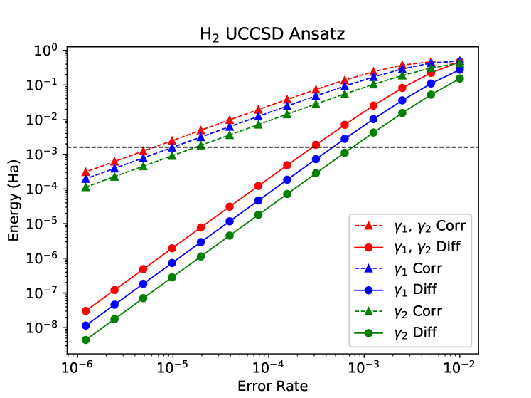
Figure 1: Error cancellation for H₂ at bond length 0.74 Å using the unitary coupled cluster singles doubles (UCCSD) ansatz, under amplitude damping ($\gamma_{1}$), dephasing ($\gamma_{2}$), and both amplitude damping and dephasing ($\gamma_{1},\gamma_{2}$) noise sources. The horizontal line represents ‘chemical accuracy’, 1.6 mHa. The dashed lines with triangle markers represent the amount of correction applied by our scheme. The solid lines with circle markers represent the difference between the corrected energy and the energy evaluated with no noise. Corrections of up to 70 mHa are applied to get to chemical accuracy and error rates can be up to 50$\times$ larger. (Error rates in this and all subsequent figures are in units of the inverse time interval between gate applications.)

Our first example is the hydrogen dimer, H₂, at equilibrium geometry (bond length 0.74 Å). We use the sto-3g basis, resulting in a four qubit circuit. We use the UCCSD ansatz (166 gates) and note that each gate is applied sequentially with one time unit between each gate; we made no effort to apply gates in parallel. The parameters of the wavefunction ansatz were optimized with noise on every qubit. We then sweep through the qubits, removing the noise from one qubit at a time, simulating the effect of error correction on just that qubit. The final energy is then calculated by using our correction scheme, Eq. (6). We plot the results for typical amplitude damping ($\gamma_{1}$) and dephasing ($\gamma_{2}$) type noises in figure 1, representing three different environmental regimes. $\gamma_{1}=\gamma_{2}$ is similar to a superconducting qubit quantum computer Kandala et al. , whereas the noise on spin Watson et al. (2018) and trapped ion Kielpinski et al. (2002) quantum computers is dominated by $\gamma_{2}$. The dashed lines with triangle markers represent the magnitude of the correction used in our correction scheme, Eq. (6). The solid lines with circle markers represent the difference between the corrected energy and the energy if every qubit were perfectly error corrected. We see that chemical accuracy (1.6 mHa, represented by the horizontal black line) can be obtained with error rates almost two orders of magnitude higher; on average, the error rates can be 45$\times$ larger. To get to chemical accuracy, corrections of 60-70 mHa are applied. Furthermore, the corrections at all error rates, even the smallest, get the answer continually closer to the fully error corrected answer. Though it has not been proved in this paper, this gives evidence that this scheme may be variational for VQE. The Appendix provides results for a different wavefunction ansatz, one similar to the entangling ansatz of Ref. Kandala et al. . The results are consistent when using this separate ansatz. The ordering of the results provides a limited sensitivity analysis for different quantum computing architectures. Similar to Ref. Sawaya et al. (2016), we note that VQE is more sensitive to amplitude damping noise than to dephasing noise.

Even though the wavefunction parameters were optimized in the presence of noise, the final energy evaluated at the different parameter sets for the fully error corrected circuit differ very little. The optimal parameters from the largest error rates only gave a difference of 1.7mHa compared to the optimal parameters from the error free optimal parameters, when both were evaluated with no noise; this is much less than the remaining error (due to noise), even after correction, for the largest error rates. Because of this, we optimize the parameters once with no noise and use those parameters for evaluation at all noise rates in the following examples.

The correction scheme presented in this work is not limited to environmental noise sources, such as those modeled by $\gamma_{1}$ and $\gamma_{2}$, and removal via error correction. The scheme is general; systems with any noise source, describable by a Lindblad superoperator, can benefit, as long as each noise source can be isolated and removed independently of all other noise sources. To demonstrate this, we applied a thermal type noise source with rate $\gamma_{th}$ and a correlated noise source with rate $\gamma_{c}$ to the H₂ UCCSD example. The results are shown in figure 2. The trends are similar to those for amplitude damping and dephasing; corrections of around 70 mHa bring the energy to within chemical accuracy at error rates almost 50 times larger than otherwise needed. Though it might be experimentally difficult, thermal noise could be reduced by selectively cooling each qubit, one at a time. The correction scheme applied to our correlated noise term reveals some subtleties of the method. Our correlated noise Lindblad, $L^{c}(\rho)=\gamma_{c}\mathcal{D}[\sigma_{1}^{\dagger}\sigma_{2}]+\gamma_{c}\mathcal{D}[\sigma_{1}\sigma_{2}^{\dagger}]$, naturally has terms from two qubits. When we sweep through the qubits, we remove all terms which involve a single qubit; this leads to the removal of each $L^{c}$ term twice, once for each qubit in each $L^{c}$. This double counting can be simply corrected by taking half of the calculated correction from each qubit. Our scheme relies on the fact that each term is removed once (and only once); as long as the noise sources of interest and their controlled removal are well understood, the scheme can be applied. If a noise source is removed twice, accounting for that allows for a good correction. In our correlated noise term, $L^{c}$, every term is removed exactly twice and the calculated correction can be simply halved. Conversely, it is also true that if exactly half the noise is removed, the correction as if all of the noise is removed can be calculated by doubling the correction. Though it might be hard to imagine that something as specific as ‘half the noise’ can be removed, this idea can be used when the noise is controllable. If the noise is increased by a controlled, known amount (say, doubled, or even just fractionally increased), for each qubit separately, the correction scheme can be applied. The ‘correction’ would be the difference between the inflated noise run and the normal noise run, scaled by the appropriate factor. This is similar in spirit to Ref. Li and Benjamin (2017), where the total noise of the system is artificially increased and the results are subsequently extrapolated to the zero noise limit.

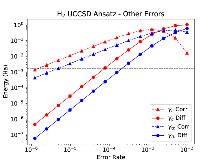
Figure 2: Error cancellation for H₂ at bond length 0.74 Å using the unitary coupled cluster singles doubles (UCCSD) ansatz under thermal noise ($\gamma_{th}$) and correlated noise ($\gamma_{c}$). The horizontal line represents ‘chemical accuracy’, 1.6 mHa. The dashed lines with triangle markers represent the amount of correction applied by our scheme. The solid lines with circle markers represent the difference between the corrected energy and the energy evaluated with no noise. Just as in amplitude damping and dephasing noise sources, corrections are as large as 70 mHa and error rates can be nearly 50$\times$ larger for chemical accuracy.

III.2 LiH

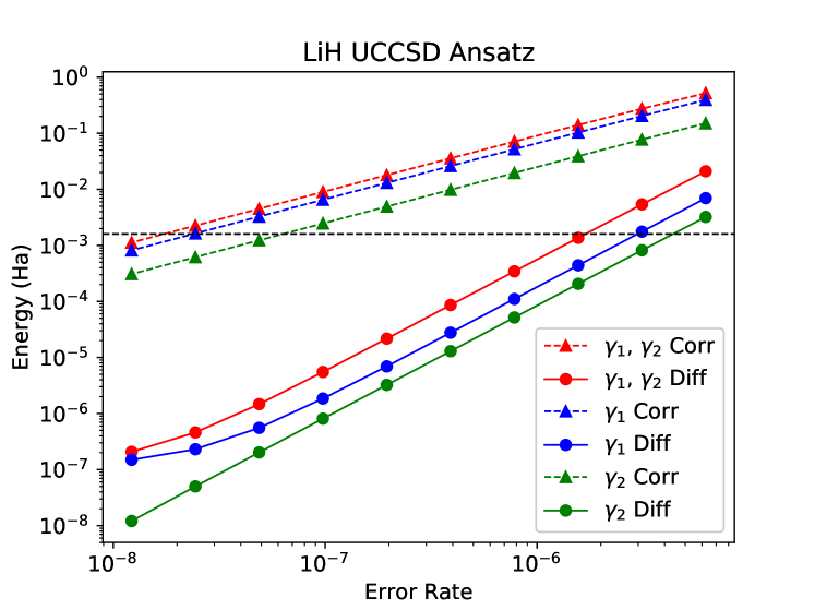
Figure 3: Error cancellation using the unitary coupled cluster singles doubles (UCCSD) ansatz for LiH, under amplitude damping ($\gamma_{1}$), dephasing ($\gamma_{2}$), and both amplitude damping and dephasing ($\gamma_{1},\gamma_{2}$) noise sources. The horizontal line represents ‘chemical accuracy’, 1.6 mHa. The dashed lines with triangle markers represent the amount of correction applied by our scheme. The solid lines with circle markers represent the difference between the corrected energy and the energy evaluated with no noise. Corrections are between 100-200 mHa and error rates can be over 100$\times$ larger for chemical accuracy.

We also studied LiH in the sto-3g basis at bond length 1.74 Å, using 12 qubits, with over 12,000 gates. We plot the results for the UCCSD ansatz in figure 3. Due to the increased number of qubits and circuit depth, the error rates are, overall, much smaller. The correction for LiH is even more dramatic than for H₂. Corrections of 100-200 mHa bring the answer to within chemical accuracy, and error rates can be over two orders of magnitude higher, ranging from 68 for with only $\gamma_{1}$ noise to 128 with only $\gamma_{2}$ noise. This example provides confidence that the correction scheme will work for larger circuits; in fact, it works even better, in this case, than for the smaller circuits of H₂. It is reasonable to believe that this will be true for ever larger circuits; the number of first order errors increases with increasing number of qubits, and these are all approximately corrected. Though the number of second order errors also increases, the second order errors go as $\gamma^{2}$ and $\tau^{2}$, and will generally be small.

IV Conclusion

We provide a simple scheme to greatly reduce the error in quantum algorithms and apply this scheme to simulations of the variational quantum eigensolver. Error correcting each qubit, one at a time, and summing the difference from the result with no error correction provides a large correction to the energy. This correction greatly reduces the coherence requirements to obtain chemical accuracy; error rates can be up to two orders of magnitude larger, without the need for full error correction. This is at a relatively low overhead; for example, just an additional $\mathcal{O}(n_{qubits})$ evaluations on the quantum computer with only single qubit error correction. This correction relies on cancellation of error between expectation values; each expectation value calculated needs a sufficient number of measurements to allow for this cancellation. On future quantum devices, either no error correction (or possibly limited error correction) on all qubits and sweeping through full error correction on each qubit can allow much larger systems to be computed, compared to full error correction on each qubit. Though we show results only for VQE, the method can reduce the error in any measured observable, and thus has application to a wide range of quantum algorithms. Further study on other algorithms, such as quantum phase estimation Kitaev (1995) and quantum approximate optimization algorithm Farhi et al. (2014), should be done to understand the impact of this scheme on other algorithms. The magnitude of the correction can also be used as a metric for measuring how close to the true answer one is, without knowing the true answer; as the correction gets smaller, the effect of the environmental noise is smaller. Furthermore, the magnitude of the correction can be used to compare different architectures, without need for knowledge of the true answer. Whichever architecture gives a smaller correction is likely closer to the true answer, and can be considered a better architecture for that problem.

V Appendix

*

Appendix A Derivation of the Observable Correction Formula

First consider the Lindbland master equation, Eq. (2). A formal solution for a density matrix evolving from time $t$ to $t+\tau$ and satisfying this equation is

$$\rho(t+\tau)=V_{\tau}(\rho(t)),$$ (7)

where

$$V_{\tau}()=\exp[\tau L()].$$ (8)

We use $()$ above to indicate that $L$ and $V$ are superoperators that take in an operator with the brackets to generate a new one. To first order in $\tau$ and taking $L()$ to be the sum over Lindblad operators of Eq. (2),

$$V_{\tau}()\approx 1+\tau\sum_{i=1}^{m}L_{i}(),$$ (9)

The sequence: apply gate 1, evolve under $V_{\tau}$, apply gate 2, etc., up to gate G corresponds exactly to a final density matrix given by

$$\rho(T)=U_{G}V_{\tau}\bigg{(}~{}U_{G-1}\cdots~{}V_{\tau}\big{(}~{}U_{2}(~{}V_{\tau}(~{}U_{1}\rho(0)U_{1}^{\dagger}~{})U_{2}^{\dagger}~{}\big{)}\cdots\\ U_{G-1}^{\dagger}~{}\bigg{)}U_{G}^{\dagger}.$$ (10)

Notice that Eq. (10) is not symmetric, with the $V_{\tau}$ operators always acting on the right side.

Equation (10) is $\rho(T)$ for the case of all $m$ error sources present. The corresponding $\rho_{a}(T)$ for perfect error correction or no error terms present is simply:

$$\rho_{a}(T)=U_{G}U_{G-1}\cdots~{}U_{2}U_{1}\rho(0)U_{1}^{\dagger}U_{2}^{\dagger}\cdots U_{G-1}^{\dagger}U_{G}^{\dagger}.$$ (11)

The density matrices resulting from removing error sources $i$ = 1,2,…, $m$ separately are

$$\rho_{i}(T)=U_{G}V_{\tau}^{i}\bigg{(}~{}U_{G-1}\cdots~{}V_{\tau}^{i}\big{(}~{}U_{2}(~{}V_{\tau}^{i}(~{}U_{1}\rho(0)U_{1}^{\dagger}~{})U_{2}^{\dagger}~{}\big{)}\cdots\\ U_{G-1}^{\dagger}~{}\bigg{)}U_{G}^{\dagger}.$$ (12)

$V_{\tau}^{i}$ is the corresponding Lindblad evolution operator that does not contain $L_{i}$ but has all other terms, e.g. to first order in $\tau$,

$$V_{\tau}^{i}()\approx 1+\tau\sum_{j\neq i}^{m}L_{j}(),$$ (13)

Now we consider the new density matrix defined as

$$\tilde{\rho}(T)=\rho(T)-\sum_{i=1}^{m}(\rho(T)-\rho_{i}(T)).$$ (14)

Insertion of the Eqs. (9) and (13) into Eq. (14) leads, after some tedious but straightforward algebraic manipulations, to

$$\tilde{\rho}(T)\approx\rho_{a}(T)$$ (15)

being correct to first order in $\tau$, i.e. all first order error terms exactly cancel, with remaining error terms on the order of $\tau^{2}$ and higher. In contrast, the uncorrected density matrix $\rho(T)$ contains first-order error terms.

Equation (14) immediately leads to the observable correction formula of the text, Eq. (6), when traced with the observable, A:

$$\begin{split}\tilde{A}&=\operatorname{Tr}(\tilde{\rho}(T)A)\\ &=\operatorname{Tr}(\rho(T)A)-\sum_{i=1}^{m}[\operatorname{Tr}(\rho(T)A)-\operatorname{Tr}(\rho_{i}(T)A)]\\ &=\langle A\rangle-\sum_{i=1}^{m}(\langle A\rangle-\langle A_{i}\rangle),\end{split}$$ (16)

which will also be accurate to order $\tau$ whereas the uncorrected observable, $\langle A\rangle$, has first order error terms.

Appendix B Entangling Ansatz for H₂

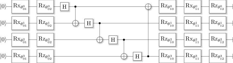
Figure 4: Single layer entangling ansatz example for four qubits.

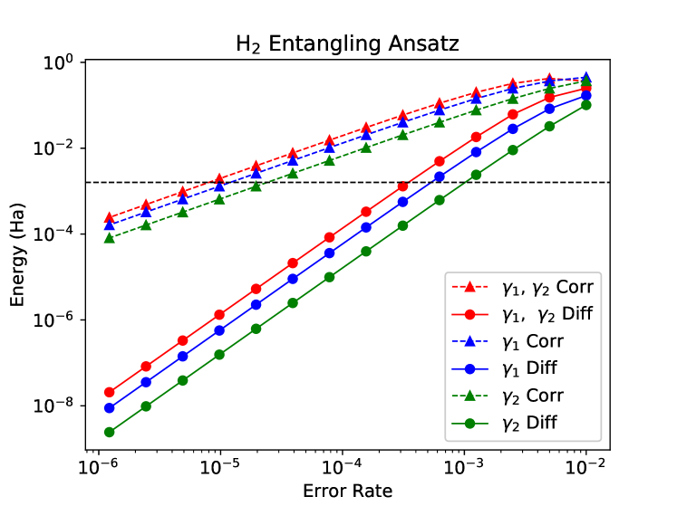
Figure 5: Error cancellation for H₂ at bond length 0.74 Å for an ‘entangling’ ansatz with 4 layers (described in the appendix), under amplitude damping ($\gamma_{1}$), dephasing ($\gamma_{2}$), and both amplitude damping and dephasing ($\gamma_{1},\gamma_{2}$) noise sources. The horizontal line represents ‘chemical accuracy’, 1.6 mHa. The dashed lines with triangle markers represent the amount of correction applied by our scheme. The solid lines with circle markers represent the difference between the corrected energy and the energy evaluated with no noise. The results are nearly the same as the unitary coupled cluster singles doubles ansatz, with corrections of up to 70 mHa applied to get to chemical accuracy and error rates which can be up to 50$\times$ larger.

We also applied our correction scheme to a different wavefunction ansatz, which we call the entangling ansatz, similar to that described in Kandala et al. . For the entangling ansatz, we parameterize the wavefunction by first applying parameterized rotations $Rx(\theta^{q}_{01})Rz(\theta^{q}_{02})$, and then alternating between entangling all the qubits in ring by applying a Hadamard gate to qubit $q$ and then a CNOT gate between qubits $q$ and $(q+1)\%n_{qubits}$ for all qubits $q$, where $\%$ is the modulo operator, followed by parameterized rotations $Rz(\theta^{q}_{i0})$, $Rx(\theta^{q}_{i1})$, and $Rz(\theta^{q}_{i2})$ for each qubit $q$ and layer $i$. This is done for a number of layers $d$. This circuit is equivalent to that described in Ref. Kandala et al. , except the entangling circuit is replaced with the ring of Hadamard - CNOTs. Figure 4 gives an example of this circuit with $d=1$. The results are shown in figure 5 for a circuit of $d=4$, and are almost indistinguishable from the UCCSD results. Corrections of up to 70 mHa are applied to get to chemical accuracy; error rates can be 50$\times$ larger to get to chemical accuracy.

References

- O’Malley et al. (2016) P. O’Malley, R. Babbush, I. Kivlichan, J. Romero, J. McClean, R. Barends, J. Kelly, P. Roushan, A. Tranter, N. Ding, et al., Physical Review X 6, 031007 (2016).
- (2) A. Kandala, A. Mezzacapo, K. Temme, M. Takita, M. Brink, J. M. Chow, and J. M. Gambetta, Nature 549, 242.
- Preskill (2018) J. Preskill, arXiv preprint arXiv:1801.00862 (2018).
- Reed et al. (2012) M. D. Reed, L. DiCarlo, S. E. Nigg, L. Sun, L. Frunzio, S. M. Girvin, and R. J. Schoelkopf, Nature 482, 382 (2012).
- Kelly et al. (2015) J. Kelly, R. Barends, A. Fowler, A. Megrant, E. Jeffrey, T. White, D. Sank, J. Mutus, B. Campbell, Y. Chen, et al., Nature 519, 66 (2015).
- Barends et al. (2014) R. Barends, J. Kelly, A. Megrant, A. Veitia, D. Sank, E. Jeffrey, T. C. White, J. Mutus, A. G. Fowler, B. Campbell, et al., Nature 508, 500 (2014).
- Fowler et al. (2012) A. G. Fowler, M. Mariantoni, J. M. Martinis, and A. N. Cleland, Physical Review A 86, 032324 (2012).
- Peruzzo et al. (2014) A. Peruzzo, J. McClean, P. Shadbolt, M.-H. Yung, X.-Q. Zhou, P. J. Love, A. Aspuru-Guzik, and J. L. O’brien, Nature communications 5, 4213 (2014).
- McClean et al. (2016) J. R. McClean, J. Romero, R. Babbush, and A. Aspuru-Guzik, New Journal of Physics 18, 023023 (2016).
- MacQuarrie et al. (2017) E. R. MacQuarrie, M. Otten, S. K. Gray, and G. D. Fuchs, Nature Communications 8, 14358 (2017).
- Otten et al. (2016) M. Otten, J. Larson, M. Min, S. M. Wild, M. Pelton, and S. K. Gray, Physical Review A 94, 022312 (2016).
- Otten et al. (2015) M. Otten, R. A. Shah, N. F. Scherer, M. Min, M. Pelton, and S. K. Gray, Physical Review B 92, 125432 (2015).
- Nielsen and Chuang (2010) M. A. Nielsen and I. L. Chuang, Quantum computation and quantum information (Cambridge university press, 2010).
- Nightingale and Umrigar (1998) M. P. Nightingale and C. J. Umrigar, Quantum Monte Carlo methods in physics and chemistry, 525 (Springer Science & Business Media, 1998).
- Kitaev (1995) A. Y. Kitaev, arXiv preprint quant-ph/9511026 (1995).
- Sawaya et al. (2016) N. P. Sawaya, M. Smelyanskiy, J. R. McClean, and A. Aspuru-Guzik, Journal of chemical theory and computation 12, 3097 (2016).
- Whitfield et al. (2011) J. D. Whitfield, J. Biamonte, and A. Aspuru-Guzik, Molecular Physics 109, 735 (2011).
- McClean et al. (2017) J. R. McClean, I. D. Kivlichan, D. S. Steiger, Y. Cao, E. S. Fried, C. Gidney, T. Häner, V. Havlíček, Z. Jiang, M. Neeley, et al., arXiv preprint arXiv:1710.07629 (2017).
- Parrish et al. (2017) R. M. Parrish, L. A. Burns, D. G. Smith, A. C. Simmonett, A. E. DePrince III, E. G. Hohenstein, U. Bozkaya, A. Y. Sokolov, R. Di Remigio, R. M. Richard, et al., Journal of chemical theory and computation 13, 3185 (2017).
- Steiger et al. (2018) D. S. Steiger, T. Häner, and M. Troyer, Quantum 2, 49 (2018).
- Otten (2017) M. Otten, “Quac: Open quantum systems in C, a time-dependent open quantum systems solver,” https://github.com/0tt3r/QuaC (2017).
- Nelder and Mead (1965) J. A. Nelder and R. Mead, The computer journal 7, 308 (1965).
- Powell (1994) M. J. Powell, in Advances in optimization and numerical analysis (Springer, 1994) pp. 51–67.
- Watson et al. (2018) T. Watson, S. Philips, E. Kawakami, D. Ward, P. Scarlino, M. Veldhorst, D. Savage, M. Lagally, M. Friesen, S. Coppersmith, et al., Nature (2018).
- Kielpinski et al. (2002) D. Kielpinski, C. Monroe, and D. J. Wineland, Nature 417, 709 (2002).
- Li and Benjamin (2017) Y. Li and S. C. Benjamin, Physical Review X 7, 021050 (2017).
- Farhi et al. (2014) E. Farhi, J. Goldstone, and S. Gutmann, arXiv preprint arXiv:1411.4028 (2014).