Chiral surface and edge plasmons in ferromagnetic conductors

Abstract

The recently introduced concept of “surface Berry plasmons” is studied in the concrete instance of a ferromagnetic conductor in which the Berry curvature, generated by spin-orbit (SO) interaction, has opposite signs for carriers parallel or antiparallel to the magnetization. By using collisionless hydrodynamic equations with appropriate boundary conditions, we study both the surface plasmons of a three-dimensional ferromagnetic conductor and the edge plasmons of a two-dimensional one. The anomalous velocity and the broken inversion symmetry at the surface or the edge of the conductor create a “handedness”, whereby the plasmon frequency depends not only on the angle between the wave vector and the magnetization, but also on the direction of propagation along a given line. In particular, we find that the frequency of the edge plasmon depends on the direction of propagation along the edge. These Berry curvature effects are compared and contrasted with similar effects induced in the plasmon dispersion by an external magnetic field in the absence of Berry curvature. We argue that Berry curvature effects may be used to control the direction of propagation of the surface plasmons via coupling with the magnetization of ferromagnetic conductors, and thus create a link between plasmonics and spintronics.

I Introduction

The discovery of collective oscillations of electrons in quantum solid-state plasmas in the 1950s was a major milestone in the evolution of condensed matter physics Pines and Nozières (1999). It exposed the fundamental dichotomy in the character of electronic elementary excitations, which can be either individual quasiparticles or organized collective oscillations (plasmons), and spawned a variety of theoretical treatments of the electron gas (the RPA Pines and Nozières (1999); Giuliani and Vignale (2005) being one of the earliest and most successful), effectively igniting the field of many-electron physics Mahan (1990). By the end of the 20th century the interest began to shift to the possible technological applications of plasmons, as it was realized that the wavelengths of these oscillations, being much shorter then the wavelength of light at the same frequency, could be used to compress electromagnetic energy to a nanometric scale – the scale of integrated circuits and devices. A thriving area of research, known as “plasmonics” Maier (2003); Stockman (2011), was born.

At about the time that plasmonics was taking off, major advances were made in the band theory of solids Ashcroft and Mermin (1976); Landau and Pitaevskii (1980). It was realized that, under quite common conditions, the Bloch wave functions of electrons in a periodic solid, regarded as functions of the Bloch wave vector $\mathbf{k}$ in the Brillouin zone, have non-trivial geometric properties. When the $n$-th eigenstate $|u_{n}(\mathbf{k})\rangle$ of the periodic Hamiltonian $H(\mathbf{k})$ is adiabatically transported around a closed loop in the Brillouin zone the final state differs from the initial one by a gauge invariant “Berry phase” $\Delta\phi$, which equals the flux of “Berry curvature” through the area enclosed by the loop Berry (1984). The mathematical expression for the Berry curvature

$$\bm{\Omega}_{n}\left(\mathbf{k}\right)=i\left\langle\nabla_{\mathbf{k}}u_{n}\left(\mathbf{k}\right)\right|\times\left|\nabla_{\mathbf{k}}u_{n}\left(\mathbf{k}\right)\right\rangle$$ (1)

is one of the most important properties of a solid-state system, its integral over the Brillouin zone being connected to topological quantum numbers and quantized conductivities Xiao et al. (2010).

A question that naturally arises at this point is: how does the Berry curvature of a band affect, if at all, the properties of the plasmons of the carriers in that band? One of the simplest ways to address the question is to set up the collisioness hydrodynamic equations for the collective motion of the electron fluid Giuliani and Vignale (2005). These will in turn be based on the quasiclassical equations of motion for wave packets in the band: Sundaram and Niu (1999); Xiao et al. (2010)

$$\mathbf{\dot{r}}=\hbar^{-1}\nabla_{\mathbf{k}}E_{n}\left(\mathbf{k}\right)+\bm{\Omega}_{n}\left(\mathbf{k}\right)\times\mathbf{\dot{k}}$$ (2a)

$$\mathbf{\dot{k}=-}\hbar^{-1}\nabla_{\mathbf{r}}V\left(\mathbf{r}\right)\,,$$ (2b)

where $$\mathbf{r} \hbar \mathbf{k} E_{n}\left(\mathbf{k}\right) V\left(\mathbf{r}\right) \mathbf{\dot{r}}$$ and   are the position and the momentum of the wave packets, is the energy of the Bloch state, and is the potential energy arising from the self-consistent electric field. The Berry curvature enters the equations of motion through the second term in the expression for . This is often referred to as the “anomalous velocity”:

$$\mathbf{v}_{a}\left(\mathbf{k}\right)\equiv\bm{\Omega}_{n}\left(\mathbf{k}\right)\times\mathbf{\dot{k}=-}\hbar^{-1}\bm{\Omega}_{n}\left(\mathbf{k}\right)\times\nabla_{\mathbf{r}}V\left(\mathbf{r}\right)\,.$$ (3)

Physically, the anomalous velocity reflects the non-conservation of the Bloch momentum. As the Bloch momentum changes under the action of a force according to Eq. (2b), the quantum state of the electron no longer coincides with the instantaneous eigenstate $\left|u_{n}\left(\mathbf{k}\left(t\right)\right)\right\rangle$.  The difference between the actual state $\left|u_{n}\left(t\right)\right\rangle$ and the instantaneous eigenstate $\left|u_{n}\left(\mathbf{k}\left(t\right)\right)\right\rangle$ is reflected in the expectation value of velocity operator $\mathbf{\hat{v}}\left(\mathbf{k}\right)\equiv\hbar^{-1}\nabla_{\mathbf{k}}\hat{H}\left(\mathbf{k}\right)$, where $\hat{H}\left(\mathbf{k}\right)$ is the Hamiltonian at wave vector $\mathbf{k}$. It is easily seen that the expectation value of $\mathbf{\hat{v}}\left(\mathbf{k}\right)$ in the instantaneous eigenstate equals $\hbar^{-1}\nabla_{\mathbf{k}}E_{n}\left(\mathbf{k}\right)$. The anomalous velocity is the correction to that result, arising from the fact that, in a dynamical situation, $\left|u_{n}\left(t\right)\right\rangle\neq\left|u_{n}\left(\mathbf{k}\left(t\right)\right)\right\rangle$.

The study of the effect of the anomalous velocity on the dynamics of the plasmons has been pioneered in a recent paper by Song and Rudner (SR) Song and Rudner (2016). Working within the framework of collisionless hydrodynamics (see Section II) they first showed that the anomalous velocity has no effect on the bulk modes of a homogeneous electron liquid. This is because the anomalous velocity enters the bulk hydrodynamics only in the continuity equation, and only through its divergence, which is zero due to $\nabla_{r}\cdot\left[\bm{\Omega}_{n}\left(\mathbf{k}\right)\times\nabla_{\mathbf{r}}V(\mathbf{r})\right]=0$.

The situation changes when one considers surface or edge plasmons Stern and Ferrell (1960). These collective oscillations are exponentially localized near the surface or the edge of the system, with a localization length of the order of $v_{F}/\omega_{p}$, where $v_{F}$ is the Fermi velocity and $\omega_{p}$ is the plasmon frequency. These are also the modes that are of greatest interest in plasmonic applications, because they hybridize with electromagnetic waves to produces surface plasmon polaritons Barnes et al. (2003); Hutter and Fendler (2004); Ebbesen et al. (2008); Pitarke et al. (2007). In the hydrodynamic approach, surface plasmons are derived by imposing a boundary condition on the current density at the surface or edge of the system. The boundary condition states that there is no electron flux through the boundary of the system,

$$j_{z}(z=0)=0\,,$$

where $z$ is the direction perpendicular to the boundary and $j_{z}$ is the $z$-component of the particle current. Notice that the imposition of the boundary condition is the way hydrodynamics - a long wavelength theory - handles the sharp variation of the electronic density across the boundary. It is precisely through the boundary condition that the anomalous velocity enters the solution for the plasmon. This point was clearly demonstrated by SR Song and Rudner (2016) for the edge plasmon of a 2D system. Taking a rather abstract approach in which a Berry curvature of unspecified origin was assumed to exist, SR showed that the frequency of right-propagating modes (along the edge) can be significantly different from that of left-propagating modes. At finite wave vector one of the two modes can be well defined while its time-reversed partner may be severely Landau-damped. Under this scenario an essentially unidirectional propagation of edge plasmons is achieved, which is of great technological interest. The scenario is similar, but not identical to that of surface and edge plasmons in a magnetic field (the so-called “magnetoplasmons”), which were studied, for example, in Refs. Chiu and Quinn (1972); Volkov and Mikhailov (1985); Fetter (1985); Ashoori et al. (1992). Both scenarios require broken time-reversal symmetry to produce chiral plasmons, but the magnetoplasmon arises from the classical Lorenz force exerted by the magnetic field, whereas the Berry plasmon arises from the anomalous velocity.

In this paper we study a concrete realization of the abstract SR scenario, namely the Berry plasmons at the surface of a ferromagnetic conductor, with the magnetization lying in the plane of the boundary surface in 3D or perpendicular to the plane of the system in 2D. Spontaneous magnetization breaks time-reversal symmetry, but we assume that the magnetic field associated with the magnetization has negligible effect on the electrons: in particular, there is no sizable Lorenz force. On the other hand, the Berry curvature of electrons in (say) the conduction band is assumed to be different from zero and spin-dependent, having opposite signs for electrons of opposite spins. For example, in the conduction band of 3D GaAs, a simple calculation based on the $8$-band model Winkler (2003) predicts the Berry curvature

$$\bm{\Omega}_{c}(\mathbf{k})\simeq\lambda^{2}\bm{\sigma}$$ (4)

at the bottom of the band. The effective Compton wavelength $\lambda$ is related to band parameters by the well-known formula

$$\lambda^{2}=\frac{2\hbar^{2}|P|^{2}}{3m_{e}^{2}}\left[\frac{1}{E_{g}^{2}}-\frac{1}{(E_{g}+\Delta)^{2}}\right]\,,$$ (5)

where $E_{g}$ is the fundamental band gap, $\Delta$ is the gap separating the light/heavy hole bands from the so-called spin-orbit (SO) split band, and $P$ is the matrix element of the momentum operator between atomic $s$ and $p$ states. Thus, the $\Delta$ gap is a direct measure of the SO-induced splitting of atomic energy levels with $J=1/2$ and $3/2$, and its non-zero value is essential to the emergence of a finite Berry curvature in the conduction band. Because electrons of opposite spins have opposite Berry curvatures, and hence opposite anomalous velocities, no effect is expected on the surface plasmons of a spin-unpolarized system. But, if the system is magnetic, then the opposite anomalous velocities of majority and minority spin electrons give a non-vanishing contribution to the net particle current, which affects the collective motion of the electron liquid, and maximally so when the electron liquid is fully spin polarized. We refer to these collective motions as ferromagnetic surface (or edge) plasmons.

The results of our study, presented below, pertain to long-wavelength plasmons (wave vector $q\ll k_{F}$, where $k_{F}$ is the Fermi wave vector), but the wavelength is not so large that retardation effects must be taken into account: namely, we assume $q\gg\omega_{p}/c$, where $c$ is the speed of light. Even in this limit, we find that the frequency of the ferromagnetic surface plasmon depends on the angle between the wave vector and the magnetization. Similarly, the frequency of the ferromagnetic edge plasmon depends on the direction of propagation along the edge. The fact that charge oscillations, such as the plasmons, “sense” the magnetization is a consequence of the spin-orbit-induced Berry curvature. It has nothing to do with the well known anisotropy of plasmons in a magnetic field. The relation between chiral magnetoplasmons and chiral ferromagnetic plasmons is reminiscent of the relation between the regular Hall effect and the anomalous Hall effect, where the former arises from the Lorentz force, while the latter arises from the concerted action of spin-orbit coupling and magnetization. Another significant difference between ferromagnetic surface plasmons and ordinary magnetoplasmons is that we find a single surface mode, as opposed to two. The two magnetoplasmons arise from the interplay of two classical forces, the electrostatic force and the Lorentz force, which can either work together or against each other. We have no Lorentz force, and therefore find a single ferromagnetic plasmon.

Chiral edge plasmons have recently been predicted Kumar et al. (2016) in two-dimensional gapped Dirac systems under pumping with circularly polarized light, which produces a population imbalance between two valleys. By contrast, the chirality of the plasmons in the present study arises from a spontaneous spin polarization under equilibrium conditions. A recent study of topological edge magnetoplasmons Jin et al. (2016) is not directly relevant to the present scenario, since it relies on a magnetic field rather than a spontaneous magnetization.

The angular dependence and chirality of the plasmon frequency is a potentially important issue in plasmonics, since it can be used to control the direction of propagation of plasmon waves. Even more interesting, in our view, is the unusual coupling between magnetism and charge oscillations that this work foreshadows. The coupling should persist in fully dynamical situations, when both the magnetization and the charge density are time dependent. This suggests the intriguing possibility of coupling plasmons and spin waves, thus bringing together the fields of spintronics Wolf et al. (2001); Žutić et al. (2004); Fabian et al. (2007); Wu et al. (2010); Awschalom and Flatté (2007) and plasmonics.

The remaining of the paper is organized as follows. In Sec. II, we introduce a hydrodynamic model of electron fluid to investigate the dispersion of surface (or edge) plamson in ferromagnetic conductors. Our treatment is based on a set of linearized hydrodynamic equations and the corresponding boundary conditions for the surface or edge plasmon modes in which the anomalous velocity comes into play. We then present the exact solution of the 3D ferromagnetic surface plasmon dispersion in Sec. III. An approximate solution of the 2D problem will be discussed in Sec. IV with a simplified treatment of the electrostatics. Following the thorough investigation of both the ferromagnetic surface and edge plamsons, we show, in Sec. V(A), that they are distinguishable from the classical surface and edge magnetoplasmons (arising from the Lorentz force) by providing a comparison between the two kinds of plasmons in the long wavelength limit. And finally in Sec. V(B), we discuss possible experimental observation of the ferromagnetic surface and edge plasmons in various ferromagnetic systems. The conclusion is given in Sec. VI.

II Collisionless hydrodynamics

Unlike proper hydrodynamics, which presupposes slow collective motion on the scale of the particle-particle collision frequency, collisionless hydrodynamics applies to high-frequency collective motion, such as plasmons, in which collisions between quasiparticle can be disregarded Pines and Nozières (1999). It is well known that the full-fledged collisionlesss hydrodynamic treatment must include a viscoelastic stress tensor, which produces not only the “hydrostatic force” (gradient of pressure), but also an elastic shear force and a viscous friction force Giuliani and Vignale (2005). These two additional forces are essential to obtain, respectively, the correct dispersion of plasmons at finite wave vector and the non-Landau damping Pines and Nozières (1999). In this paper, however, we limit ourselves to a more crude model, in which we neglect shear and viscous forces. This approach is expected to become essentially exact in the long wavelength limit, due to the dominance of electrostatic forces, but will become inaccurate at shorter wavelength. These inaccuracies are of secondary importance here, since our primary interest is in the qualitatively new features of the solution, which appear already in the long wavelength limit. With the above discussion in mind, the bulk hydrodynamic equations are

$$\partial_{t}\delta n+\nabla\cdot\mathbf{j}=0$$ (6)

(continuity equation) and

$$\partial_{t}\mathbf{j}_{p}+s^{2}\nabla\delta n-\frac{en_{0}}{m_{e}}\nabla\varphi=0$$ (7)

the Euler equation, where $n_{0}$ is the uniform equilibrium density of electrons, $m_{e}$ is the effective mass,

$$\mathbf{j}_{p}=\frac{\mathbf{p}}{m_{e}}$$ (8)

is the canonical current density, proportional to the canonical momentum density $\mathbf{p}$, associated with the momentum variable $\hbar\mathbf{k}$, $s$ is the velocity of the hydrodynamic sound (this is of the order of the Fermi velocity, and is related to the bulk modulus $K$ by the well-known relation $s^{2}=\frac{K}{n_{0}m_{e}}$), $\delta n$ is the deviation of the electron density from the equilibrium density and $\mathbf{j}$ is the physical current density given by

$$\mathbf{j}=\mathbf{j}_{p}+\frac{\mathcal{P}n_{0}e}{\hbar}\lambda^{2}\mathbf{\hat{m}\times}\nabla\varphi$$ (9)

with $\hat{\mathbf{m}}$ being the unit vector along the magnetization, and $\mathcal{P}=\frac{n_{0\uparrow}-n_{0\downarrow}}{n_{0}}$ the spin polarization of the electron density. The hydrodynamic equations contain the electrostatic potential $\varphi$, which is assumed to be instantaneously created by the charge density according to the Poisson equation

$$\nabla^{2}\varphi=4\pi e\delta n\,.$$ (10)

The solution of the Poisson equation is straightforward in 3D, but not at all in 2D, unless some simplifying approximations are made, which we will discuss later.

In the absence of boundary conditions it is easy to see that the solution to the hydrodynamic equations (together with the Poisson equation) is not affected by the anomalous velocity. This is because, as remarked in the introduction, $\nabla\cdot(\hat{\mathbf{m}}\times\nabla\varphi)=0$ allows us to replace $\mathbf{j}$ by $\mathbf{j}_{p}$ in the continuity equation. Then the coupled equations for $\delta n$ and $\mathbf{p}$ do not contain the anomalous term and therefore the eigenfrequencies do not depend on $\lambda$ or $\hat{\mathbf{m}}$. On the other hand, for surface or edge modes the boundary condition of vanishing charge current density, i.e., $\left.\mathbf{j}_{z}\right|_{z=0^{-}}=0$, creates a coupling between charge and magnetization; this boundary condition can be explicitly written as

$$\left[\mathbf{j}_{p,z}+\frac{e\mathcal{P}n_{0}}{\hbar}\lambda^{2}\left(\mathbf{\hat{m}\times}\nabla\varphi\right)\cdot\mathbf{\hat{z}}\right]_{z=0^{-}}=0\,.$$ (11)

In addition, the electric potential and its gradient must be continuous at $z=0$, i.e.,

$$\left.\varphi\right|_{z=0^{-}}=\left.\varphi\right|_{z=0^{+}}\text{ and }\left.\partial_{z}\varphi\right|_{z=0^{-}}=\left.\partial_{z}\varphi\right|_{z=0^{+}}\,.$$ (12)

III Solution in three dimensions

Assuming translational invariance in the plane of the surface, we seek solutions in the form of plane waves of wave vector $\mathbf{q}$ decaying exponentially in the bulk ($z<0$) as $e^{\kappa z}$ with $\kappa>0$. We let all the physical quantities (e.g., $\delta n$, $\mathbf{p}$ and $\varphi$) take the form $\Psi\left(\mathbf{r},z;t\right)\sim e^{\kappa z}e^{i(\mathbf{q}\cdot\mathbf{r}-\omega t)}$ up to some constant coefficients to be determined by the boundary conditions. Notice that boldface symbols are use to indicate vectors in the plane of the surface. Inserting this ansatz in the hydrodynamic equations we find a set of homogeneous algebraic equations, i.e.,

$$-i\omega\delta n+\kappa j_{p,z}+i\mathbf{q}\cdot\mathbf{j}_{p,\parallel}=0$$ (13a)

$$-i\omega j_{p,z}+s^{2}\kappa\delta n-\frac{en_{0}}{m_{e}}\kappa\varphi=0$$ (13b)

$$-i\omega\mathbf{j}_{p,\parallel}+i\mathbf{q}s^{2}\delta n-i\mathbf{q}\frac{en_{0}}{m_{e}}\varphi=0\,,$$ (13c)

where $$\mathbf{j}_{p,\parallel}=\left(j_{p,x},j_{p,y}\right) \varphi \delta n$$ are the in-plane components of the particle current density, and and are related by

$$\varphi=\frac{4\pi e\delta n}{\kappa^{2}-q^{2}}$$ (14)

through the Poisson equation. The set of equations has nontrivial solutions only if

$$\kappa^{2}=q^{2}+s^{-2}\left(\omega_{B}^{2}-\omega^{2}\right)\,,$$ (15)

where $\omega_{B}^{2}=\frac{4\pi e^{2}n_{0}}{m_{e}}$ is the bulk plasmon frequency.

Now we can write down the general solution for the density oscillation as

$$\delta n=\delta n_{1}e^{\kappa z}e^{i\mathbf{q}\cdot\mathbf{r}}\,,~{}~{}~{}z<0$$ (16)

and that for the electric potential as

$$\varphi = \varphi_{1}e^{\kappa z}e^{i\mathbf{q}\cdot\mathbf{r}}+\varphi_{2}e^{qz}e^{i\mathbf{q}\cdot\mathbf{r}}\text{, \ \ }z<0$$

$$\varphi = \varphi_{0}e^{-qz}e^{i\mathbf{q}\cdot\mathbf{r}}\text{, \ }z>0$$ (17)

with $\delta n_{1}$, $\varphi_{0}$, $\varphi_{1}$, and $\varphi_{2}$ being integration constants to be determined by the boundary conditions.

Putting the general solutions for the electron density fluctuation (16) and the electric potential (17) into the boundary conditions given by Eqs. (11) and (12), we obtain a set of three linear homogeneous equations, the solution of which gives the dispersion relation

$$\left(\kappa+q\right)\omega_{B}^{2}-2\kappa\omega^{2}+\mathcal{P}\left(\kappa-q\right)\omega_{B}^{2}\omega\tau_{so}\sin\phi_{q}=0\,,$$ (18)

where $\phi_{q}$, with $-\pi<\phi_{q}\leq\pi$, is the angle between the wave vector $\mathbf{q}$ and the in-plane magnetization, and the quantity $\tau_{so}\left(\equiv\frac{m_{e}\lambda^{2}}{\hbar}\right)$ has the dimension of time which characterizes the strength of the SO interaction. Making use of Eq. (15), one can rewrite Eq. (18) as follows

$$\left(\kappa-q\right)\left[\omega^{2}-s^{2}\left(\kappa+q\right)^{2}-\mathcal{P}\omega_{B}^{2}\omega\tau_{so}\sin\phi_{q}\right]=0\,.$$ (19)

While the solution $\kappa=q$ gives the bulk frequency of $\omega=\omega_{B}$ as can be easily seen from Eq. (15), the general surface plasmon frequency is given by the equation

$$\omega^{2}-s^{2}\left(\kappa+q\right)^{2}-\mathcal{P}\omega_{B}^{2}\omega\tau_{so}\sin\phi_{q}=0\,.$$ (20)

It is instructive to first examine the solutions in the long wavelength limit ($q\rightarrow 0$) for which Eq. (20) reduces to

$$2\omega^{2}-\omega_{B}^{2}-\mathcal{P}\omega_{B}^{2}\omega\tau_{so}\sin\phi_{q}=0\,.$$ (21)

Equation (21) has two possible solutions

$$\omega_{+}=\frac{\omega_{S}}{2}\left[\mathcal{P}\omega_{S}\tau_{so}\sin\phi_{q}+\sqrt{4+\left(\mathcal{P}\omega_{S}\tau_{so}\sin\phi_{q}\right)^{2}}\right]$$ (22a)

$$\omega_{-}=\frac{\omega_{S}}{2}\left[\mathcal{P}\omega_{S}\tau_{so}\sin\phi_{q}-\sqrt{4+\left(\mathcal{P}\omega_{S}\tau_{so}\sin\phi_{q}\right)^{2}}\right]\,,$$ (22b)

where $$\omega_{S}=\frac{\omega_{B}}{\sqrt{2}} q=0 \phi_{q} \omega_{+} \omega_{-} \omega_{+}\left(-\phi_{q}\right)=-\omega_{-}\left(\phi_{q}\right). \mathbf{q} q \phi_{q} \omega_{+}(\mathbf{q}) \mathbf{q} e^{i\mathbf{q}\cdot\mathbf{r}}e^{-i\omega_{+}(\mathbf{q})t}+e^{-i\mathbf{q}\cdot\mathbf{r}}e^{-i\omega_{-}(-\mathbf{q})t} \phi_{q} \mathbf{q} -\mathbf{q} e^{-i\mathbf{q}\cdot\mathbf{r}}e^{-i\omega_{+}(-\mathbf{q})t}+e^{i\mathbf{q}\cdot\mathbf{r}}e^{-i\omega_{-}(\mathbf{q})t} \mathbf{q} -\mathbf{q} \tau_{so} \mathcal{P}$$ is the 3D surface plasmon frequency at . We observe that, for any angle , the solution is positive whereas the solution is negative. Moreover, the solutions satisfy the relation The existence of two solutions connected in this manner is a necessary condition for being able to construct real solutions of the hydrodynamic equations. Physically, the two solutions together describe a single chiral wave whose frequency is determined, for each wave vector (specified by its magnitude and angle ) by the positive branch . A real wave that propagates in the direction of is described by the superposition , where we have used the fact that changing the sign of amounts to reversing the direction of . Similarly, a real wave that propagates in the direction of is described by the superposition . Crucially, the two waves, with wave vectors and respectively, exhibit different phase velocities, and different dependences on material parameters such as the strength of the SO interaction characterized , spin polarization , etc.

Another interesting feature of the 3D ferromagnetic surface plasmon is that the decay length $\kappa^{-1}$ behaves quite differently for waves that propagate in opposite directions. More specifically, if the decay length $\kappa^{-1}$ evaluated from Eq. (15) with $\omega=\omega_{+}(\mathbf{q})$ increases with increasing value of $\left|\mathcal{P}\omega_{S}\tau_{so}\right|$ for surface plasmons propagating along $\mathbf{q}$ direction, then it must decrease with increasing value of $\left|\mathcal{P}\omega_{S}\tau_{so}\right|$ for those propagating along $-\mathbf{q}$ direction. This can be easily observed in the long wavelength limit for which $\omega_{+}$ is explicitly given by Eq. (22a). Furthermore, we note that when the product $\left|\mathcal{P}\omega_{S}\tau_{so}\right|$ becomes sufficiently large, the surface plasmon mode is forbidden in a range of directions where $\kappa$ remains imaginary (physically this means that the surface mode merges with the bulk mode in these directions). For the long wavelength limit, one can show that when $\left|\mathcal{P}\omega_{S}\tau_{so}\right|>\frac{1}{\sqrt{2}}$, there exist two intervals for the plasmon propagation angle $\phi_{q}\in\left[\phi_{q}^{crit}-\pi,-\phi_{q}^{crit}\right]\cup\left[\phi_{q}^{crit},\pi-\phi_{q}^{crit}\right]$ with $\phi_{q}^{crit}=\arcsin\left(\frac{1}{\sqrt{2}\left|\mathcal{P}\omega_{S}\tau_{so}\right|}\right)$, in which surface mode is absent, as shown schematically in Fig. 1(d).

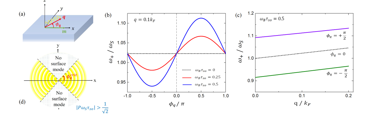
Figure 1: Variation of the 3D ferromagnetic surface plasmon frequency $\omega_{+}$ (scaled by $\omega_{S}$) with the in-plane wave vector $\mathbf{q}$. The set-up of the system is shown schematically in panel (a) with $\phi_{q}$ defined as the angle between the direction of propagation of the surface plasmon and the direction of magnetization fixed on the $x$-axis. Panel (b) shows $\omega_{+}$ as a function of $\phi_{q}$ at a fixed magnitude of the wave vector of $q=0.1k_{F}$ for several different values of $\tau_{so}$ (scaled by $\omega_{B}^{-1}$), panel (c) shows $\omega_{+}$ as a function of the magnitude of the wave vector $q$ for several different angles $\phi_{q}$ with a given SO interaction strength $\omega_{B}\tau_{so}=0.5$, and panel (d) is a schematic picture showing the range of $\phi_{q}$ (plasmon propagation directions) for which the surface mode is forbidden when the quantity $\left|\mathcal{P}\omega_{S}\tau_{so}\right|$ is greater than $\frac{1}{\sqrt{2}}$.

In Fig. 1, we show the ferromagnetic surface plasmon frequency as a function of the direction and the magnitude of the wave vector $\mathbf{q}$. For a given $q\left(=0.1k_{F}\right)$, the surface plasmon frequency exhibits a sinusoidal-like dependence on $\phi_{q}$ as shown in Fig. 1(b): It reaches a maximum at $\phi_{q}=+\frac{\pi}{2}$ and a minimum at $\phi_{q}=-\frac{\pi}{2}$ (i.e., when the surface plasmon propagates in directions perpendicular to the magnetization), and coincides with the normal surface plasmon frequency in the absence of SO interaction (indicated by the black dotted line) when the surface plasmon propagates parallel or antiparallel to the magnetization (i.e., $\phi_{q}=0$ or $\pi$).

Fig. 1(c) shows the surface plasmon frequency as a function of the magnitude of the plasmon wave vector for three different directions of propagation, $\phi_{q}=-\frac{\pi}{2},0,\frac{\pi}{2}$. We note that while $\omega_{+}$ grows monotonically with $q$ for all three directions, their frequencies remain non-degenerate for any $q$ due to the presence of the SO interaction. One interesting consequence of the anisotropic dispersion is that the phase velocities, given by $\frac{\omega_{+}(\mathbf{q})}{q}$, for surface plasmons propagating in opposite directions ($\phi_{q}\neq 0,\pi$) are always different: this implies that as long as the direction of propagation deviates from the direction of the magnetization, no standing wave can be formed for surface plasmons.

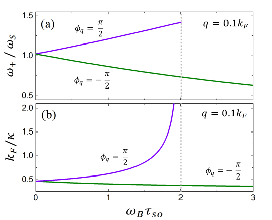
Figure 2: Dependence of 3D ferromagnetic surface plasmon on the strength of the SOC (characterized by $\omega_{B}\tau_{so}$): (a) The ferromagnetic surface plasmon frequency $\omega$ (scaled by $\omega_{S}$) as a function of $\omega_{B}\tau_{so}$ and (b) the decay length of the surface mode given by $\kappa^{-1}$ as a function of $\omega_{B}\tau_{so}$ at a given magnitude of wave vector $q=0.1k_{F}$, including two opposite propagation directions: $\phi_{q}=\frac{\pi}{2}$ and $-\frac{\pi}{2}$ respectively.

In Fig. 2, we show the dependences of the frequency $\omega_{+}$ and decaying length $\kappa^{-1}$ of the surface plasmons on the strength of the SO interaction characterized by $\omega_{B}\tau_{so}$. As the effect of the SO interaction is most prominent for surface plasmons propagating in the directions perpendicular to the magnetization, we shall focus on the cases of $\phi_{q}=-\frac{\pi}{2}$ and $\frac{\pi}{2}$ for a finite magnitude of the wave vector $q$. Consistent with the qualitative analysis we performed for the long wave length limit, we find that for surface plasmons propagating at an angle $\phi_{q}=-\frac{\pi}{2}$ with respect to the magnetization, both $\omega_{+}$ and $\kappa^{-1}$ decrease monotonically with increasing $\omega_{B}\tau_{so}$, whereas for those propagating in the opposite direction (i.e., $\phi_{q}=\frac{\pi}{2}$) both $\omega_{+}$ and $\kappa^{-1}$ increase monotonically with increasing $\omega_{B}\tau_{so}$ and are terminated when $\tau_{so}$ reaches a certain threshold (indicated by the vertical dashed line in the Fig. 2) where the decay length $\kappa^{-1}$ diverges as $\omega^{2}$ approaches $\omega_{B}^{2}+s^{2}q^{2}$ (cf. Eq. (15)) and the surface mode merges into the bulk mode .

IV Solution in two dimensions

An exact treatment of the electrostatics in a two-dimensional plane is quite more complicated than in 3D, due to the fact that the electric field exists in the whole three-dimensional space, while the electron density is confined to a plane. Fortunately, the treatment can be greatly simplified by making the approximation adopted by Fetter Fetter (1985) in his treatment of the two-dimensional edge magnetoplasmon, namely replacing the exact electrostatic Green’s function (the nonlocal kernel that connects the density to the potential in the plane) by an approximate Green’s function that has the same integrated area and second moment. What is lost in the approximation is a weak logarithmic dependence of the edge magnetoplasmon frequency on the magnitude of the wave vector, $\omega\sim q|\ln q|$, which is confirmed by a more accurate treatment making use of the Wiener-Hopf technique. Volkov and Mikhailov (1985); Noble (1958) This is not a very serious drawback in our case, since the long wavelength dispersion continues to be largely controlled by classical electrostatics, which mandates a $\sqrt{q}$ dependence. With this approximation, the equations remain essentially the same as in 3D, except that Eq. (LABEL:Eq:w2D-gen1), connecting the potential to the density, takes the slightly different form

$$\varphi=\frac{4\pi e|q|}{\kappa^{2}-2q^{2}}\delta n\,.$$ (23)

We let the electron liquid be confined to the $y$-$z$ plane, and consider the edge plasmon localized in the $z$-direction and propagating in the $y$-direction, while the magnetization is along the $x$ axis, perpendicular to the electron liquid (since the plasmon only propagates in the $y$-direction, we have suppressed the subscript for the wave vector $q.$). Combining Eq. (23) with the set of equations (13a-13c) (with $\mathbf{q}$ replaced by $q\mathbf{\hat{y}}$), we arrive at the equation relating the edge plasmon frequency $\omega$ and the decaying constant $\kappa$, i.e.,

$$\kappa^{4}-\kappa^{2}\left(k_{0}^{2}+k_{\omega}^{2}+3q^{2}\right)+2q^{2}\left(k_{\omega}^{2}+q^{2}\right)=0\,,$$ (24)

where we have defined

$$k_{\omega}^{2}\equiv\frac{\omega_{q}^{2}-\omega^{2}}{s^{2}}\text{ and }k_{0}^{2}\equiv\frac{\omega_{q}^{2}}{s^{2}}\,$$ (25)

with $\omega_{q}=\sqrt{\frac{2\pi n_{0}e^{2}\left|q\right|}{m_{e}}}$ the bulk 2D plasmon frequency. The equation has two solutions:

$$\kappa_{1,2}^{2} = \frac{1}{2}\left[k_{0}^{2}+k_{\omega}^{2}+3q^{2}\right.$$ (26)

$$\left.\pm\sqrt{\left(k_{0}^{2}+k_{\omega}^{2}\right)^{2}+q^{2}\left(6k_{0}^{2}-2k_{\omega}^{2}+q^{2}\right)}\right]\,.$$

Similar to the 3D case, we write the general solutions for the electrostatic potential and the electron density fluctuation as follows

$$\varphi = \varphi_{1}e^{\kappa_{1}z}e^{iqy}+\varphi_{2}e^{\kappa_{2}z}e^{iqy}\text{, \ \ }z<0$$

$$\varphi = \varphi_{0}e^{-\sqrt{2}qz}e^{iqy}\text{, \ }z>0$$ (27)

$$\delta n=\frac{1}{4\pi e\left|q\right|}\left[\left(\kappa_{1}^{2}-2q^{2}\right)\varphi_{1}e^{\kappa_{1}z}+\left(\kappa_{2}^{2}-2q^{2}\right)\varphi_{2}e^{\kappa_{2}z}\right]e^{iqy}\,,$$ (28)

where we have suppressed the common time-dependent components. The general solution for the density fluctuation $\delta n$ was derived by invoking the approximate Poisson relation (23). Putting these equations in the boundary conditions, we derive the following equation for $\omega$, the solution of which gives the edge plasmon frequency, i.e.,

$$\frac{\kappa_{1}\left(\kappa_{1}^{2}-2q^{2}-2k_{0}^{2}\right)+2\mathcal{P}k_{0}^{2}\omega\tau_{so}qm_{x}}{\kappa_{2}\left(\kappa_{2}^{2}-2q^{2}-2k_{0}^{2}\right)+2\mathcal{P}k_{0}^{2}\omega\tau_{so}qm_{x}} = \frac{\kappa_{1}+\sqrt{2}\left|q\right|}{\kappa_{2}+\sqrt{2}\left|q\right|}\,.$$

Note that the magnetization enters the dispersion relation only through the $x$-component of the magnetization (i.e., the one perpendicular to the plane of the 2D electron liquid). This can be understood as follows: The magnetization enters the formula for the anomalous velocity as $\mathbf{v}_{a}\sim\mathbf{\hat{m}\times}\nabla\varphi$; as the surface plasmon propagates along the edge in the $y$-direction, only the $x$-component of the magnetization generates an anomalous velocity in the $z$-direction (perpendicular to the edge), which affects the boundary condition and hence the edge plasmon frequency.

In the long wavelength limit, we obtain simpler forms for $\kappa_{1}$ and $\kappa_{2}$ by keeping only leading order terms in $q$, i.e.,

$$\kappa_{1}\simeq C_{\omega}\left|q\right|+O\left(q^{3}\right)$$ (30)

with $C_{\omega}^{2}=\frac{\omega_{q}^{2}-\omega^{2}}{\omega_{q}^{2}-\frac{1}{2}\omega^{2}}$ and

$$\kappa_{2}\simeq\frac{1}{s}\sqrt{2\omega_{q}^{2}-\omega^{2}}+O\left(q^{2}\right)\,.$$ (31)

Making use of these expressions, the general equation (LABEL:Eq:w2D-gen1) can be reduced to

$$\omega^{2}-\frac{2}{3}\omega_{q}^{2}+\frac{2\sqrt{2}}{3}\mathcal{P}\omega_{q}^{2}\omega\tau_{so}m_{x}=0\,,$$ (32)

where we have made the approximation of $C_{\omega}\simeq\frac{\sqrt{2}}{2}$ by taking $\omega$ to be the unperturbed edge plasmon frequency $\omega^{\left(0\right)}=\sqrt{\frac{2}{3}}\omega_{q}$. Fetter (1985) This equation has two solutions,

$$\omega_{+}=\frac{\sqrt{2}}{3}\omega_{q}\left[\sqrt{3+\left(\mathcal{P}\omega_{q}\tau_{so}m_{x}\right)^{2}}-\mathcal{P}\omega_{q}\tau_{so}m_{x}\mathrm{sgn}\left(q\right)\right]$$ (33)

and

$$\omega_{-}=-\frac{\sqrt{2}}{3}\omega_{q}\left[\sqrt{3+\left(\mathcal{P}\omega_{q}\tau_{so}m_{x}\right)^{2}}+\mathcal{P}\omega_{q}\tau_{so}m_{x}\mathrm{sgn}\left(q\right)\right]\,.$$ (34)

Notice that in the absence of the SO interaction, we recover the unperturbed edge plasmon frequency. As in the 3D case, the reality of the classical wave fields requires $\omega_{+}\left(-q\right)=-\omega_{-}\left(q\right)$, which shows the solutions of opposite frequencies and momenta to be parts of the same wave. Also, reversing the direction of propagation of the edge plasmon is equivalent to reversing the direction of the magnetization direction: therefore we find $\omega_{+}\left(-\mathbf{m}\right)=-\omega_{-}\left(\mathbf{m}\right)$ as expected. For this reason, we shall concentrate on the positive solution $\omega_{+}$ of the 2D ferromagnetic edge plasmons in the following discussions.

Properties of the 2D ferromagnetic edge plasmon at finite wavelength are readily obtained by numerically solving Eq. (LABEL:Eq:w2D-gen1). In Fig. 3(a), we plot $\omega_{+}$ as a function of wave vector $q$ with the magnetization direction fixed along the $x$-axis. In the absence of the SO interaction (i.e., $\omega_{k_{F}}\tau_{so}=0$), $\omega_{+}$ is symmetric in $q$ as indicated by the black dotted lines. The frequency of the left-propagating mode increases with increasing strength of the SO interaction, whereas that of the right-propagating mode decreases. In addition, we observe that the left- and right-propagating modes remain gapless at $q=0$, in contrast to the 2D edge magnetoplasmon Fetter (1985), which develops a gap in one direction. We will come back to this point in the next section when we compare the ferromagnetic surface plasmon with the more familiar surface magnetoplasmon. A similar chiral plasmon dispersion was also found in massive Dirac systems Kumar et al. (2016).

In Fig. 3(b), we plot $\omega_{+}$ as a function of the polar angle $\theta_{M}$ between the magnetization and the $x$-axis for a right-propagating wave with a given wave vector of $q=0.1k_{F}$ where $k_{F}$ is the Fermi wavelength. The extremes in $\omega_{+}$ occur when the magnetization is perpendicular to the plane of the 2D electron fluid with a maximum at $\theta_{M}=\pi$ and a minimum at $\theta_{M}=0$. The SO interaction has no effect on the edge ferromagnetic plasmon when the magnetization lies in the plane of the 2D electron fluid as shown by the crossing point at $\theta_{M}=\frac{\pi}{2}$.

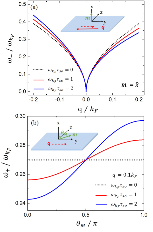
Figure 3: Dependence of the 2D ferromagnetic edge plasmon frequency (scaled with bulk plasmon frequency with $q=k_{F}$) on (a) the wave vector along the $y$-direction with magnetization direction (denoted by $\mathbf{m}$) fixed in the $x$-direction and (b) angle $\theta_{M}$ between the magnetization $\mathbf{m}$ and the $x$-direction (i.e., the normal direction of 2D electron liquid plane), including three different strengths of the SO interaction.

Lastly in Fig. 4, we show the variations of the frequency $\omega_{+}$ and decaying lengths $\kappa_{1}^{-1}$ and $\kappa_{2}^{-1}$, given by Eq. (26) ), as functions of the strength of the SO interaction. For the right-propagating mode (i.e., $q=0.1k_{F}$), both $\omega_{+}$ and $\kappa_{i}^{-1}$ ($i=1,2$) decrease with increasing $\omega_{k_{F}}\tau_{so}$, whereas for left-propagating mode (i.e., $q=-0.1k_{F}$) both $\omega_{+}$ and $\kappa_{i}^{-1}$ ($i=1,2$) increase monotonically with increasing $\omega_{k_{F}}\tau_{so}$ and terminate, similar to the 3D case, when $\omega_{k_{F}}\tau_{so}$ reaches a threshold (as indicated by the vertical dashed line) beyond which the edge mode merges with the bulk mode.

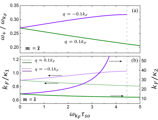
Figure 4: (a) Variation of the edge ferromagnetic surface plasmon frequency $\omega$ vs SO interaction strength parameter $\omega_{k_{F}}\tau_{so}$ and (b) variation of the decay lengths of the edge modes $\kappa_{1,2}^{-1}$ vs $\omega_{k_{F}}\tau_{so}$. Two opposite wave vectors $q=0.1k_{F}$ and $q=-0.1k_{F}$ are considered. The vertical grey dashed lines indicate the critical magnitude of the SO interaction beyond which the edge mode with $q=-0.1k_{F}$ no longer exists.

V Discussion

V.1 Comparison with surface and edge magnetoplasmon

Now that we have thoroughly investigated both the surface and edge plasmons in 3D and 2D ferromagnetic conductors, it is worthwhile discussing the features that distinguish them from the classical surface or edge magnetoplasmons. In the classic magnetoplasmon, the direction dependence of the plasmon dispersion arises from the Lorentz force exerted by the applied magnetic field, while in the present case there is no magnetic field, but an anomalous velocity connecting the collective charge oscillation with the bulk magnetization. In addition, we note that the anomalous velocity term plays a role in altering surface ferromagnetic plasmon frequency only through the boundary conditions, whereas the Lorentz force contributes to the time rate of change of the canonical current (or momentum) density and hence enters the bulk Euler equation Fetter (1985). These essential differences are reflected in the dispersion relations. Qualitative differences emerge already in the long wavelength limit, as we show below.

For a surface magnetoplasmon that propagates in the $(x,y)$ plane, with magnetic field lying in the same plane, the $q\rightarrow 0$ limit of the dispersion is given by

$$\omega_{mp}^{3D}(\phi_{q})=\frac{\omega_{c}\sin\phi_{q}}{2}+\sqrt{\frac{\omega_{c}^{2}\sin^{2}\phi_{q}}{4}+\frac{\omega_{B}^{2}+\omega_{c}^{2}\cos^{2}\phi_{q}}{2}}\,,$$ (35)

where $\omega_{c}\left(>0\right)$ is the cyclotron frequency and $\phi_{q}$ is the angle between $\mathbf{q}$ and the applied magnetic field. A detailed derivation of surface magnetoplasmon dispersion with arbitrary propagation direction is presented in Appendix A. For plasmons propagating perpendicular to the in-plane magnetic field, i.e., $\phi_{q}=\pm\frac{\pi}{2}$, Eq. (35) reduces to

$$\omega_{mp,\perp}^{3D}=\frac{1}{2}\left(\sqrt{\omega_{c}^{2}+2\omega_{B}^{2}}\pm\omega_{c}\right)\,.$$ (36)

which is exactly the result for the special case discussed by Fetter Fetter (1985). The general dispersion (35) also shows that even when the plasmon wave vector is collinear with the magnetic field (i.e., when $\phi_{q}=0$), the magnetic field still gives rise to a correction to the surface magnetoplasmon frequency of second order in $\omega_{c}$, i.e.,

$$\omega_{mp,\parallel}^{3D}=\sqrt{\frac{\omega_{B}^{2}+\omega_{c}^{2}}{2}}\,,$$ (37)

This may seem a little counterintuitive at first glance as one may think the Lorentz force, given by $\frac{e}{c}\mathbf{j\times H}\$with $\mathbf{H}$ and $\mathbf{j}$ the magnetic field and the current density respectively, would vanish in this geometry; however, this is in fact not the case since the in-plane current density is in general not parallel to the wave vector in the presence of the magnetic field (see Appendix A for the general relation between $\mathbf{j}$ and $\mathbf{q}$: the component of the electric field perpendicular to the surface combines with the magnetic field to produce a drift velocity perpendicular to the magnetic field). In addition, due to mirror symmetry about the plane perpendicular to the magnetic field, the frequencies of surface plasmons propagating parallel or antiparallel to the applied magnetic field must be identical, giving rise to an effect of the order of $O\left(\omega_{c}^{2}\right)$. Although the frequency of the ferromagnetic surface plasmons also remains finite at $q=0$, it reduces to the normal surface plasmon frequency of $\omega_{S}=\frac{\omega_{B}}{\sqrt{2}}$ when the propagation direction of the plasmon waves become collinear with the in-plane magnetization (i.e., $\phi_{q}=0$ or $\pi$). The reason for this different behavior is that the anomalous velocity ceases to be operative in the boundary condition for the current density when $\mathbf{q}$ is parallel to $\hat{\mathbf{m}}$ (see Eq. (11). Another difference is that surface magnetoplasmons in the long wavelength limit remain well defined for all directions of $\mathbf{q}$ and all values of the magnetic field, at variance with ferromagnetic plasmons which in certain directions may merge with the bulk plasmons when the SO interaction is strong enough.

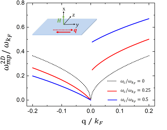
Figure 5: 2D edge magnetoplasmon dispersion relation with the external magnetic field (denoted by $\mathbf{H}$) fixed in the $x$-direction, for three different magnitudes of $\mathbf{H}$.

More significant differences arise in two dimensions. Quoting from Ref. Fetter, 1985 the dispersion of the low-frequency edge magnetoplasmon for $q\rightarrow 0$ is

$$\omega_{mp}^{2D}=\frac{\sqrt{2}}{3}\left[\sqrt{3\omega_{q}^{2}+\omega_{c}^{2}}+\omega_{c}sgn\left(q\right)\right],$$ (38)

where $\omega_{c}>0$ is the cyclotron frequency, and $\omega_{q}\left(=\sqrt{\frac{2\pi n_{0}e^{2}\left|q\right|}{m_{e}}}\right)$ is the bulk 2D plasmon frequency. We see that in this case the right-propagating mode with $q>0$ is gapped and approaches a frequency $\frac{2\sqrt{2}}{3}\omega_{c}$ in the long wavelength limit, whereas the left-propagating mode with $q<0$ has a frequency that goes to zero linearly for $q\rightarrow 0$, as shown in Fig. 5. This is quite different from the ferromagnetic edge plasmons, where both right- and left propagating waves have a dispersion $\omega\propto\omega_{q}\propto\sqrt{q}$ for $q\rightarrow 0$, only with different proportionality constants in the two directions, as shown by Fig. 3(a).

V.2 Material considerations

In transition metal ferromagnets, contributions to the anomalous Hall effect due to the intrinsic or side jump mechanism can be attributed to an anomalous velocity Nagaosa et al. (2010) which, in the present paper, has been shown to play an essential role in imparting chiral properties to the ferromagnetic surface plasmons. Consequently, one would expect the ferromagnetic surface plasmons to be observable in transition metal ferromagnets with large anomalous Hall effect. To obtain some order of magnitude estimate for the anisotropy of the ferromagnetic surface plasmon frequency in the long wavelength limit, as parameterized by $\eta_{S}\equiv\frac{\omega\left(\phi_{q}=\frac{\pi}{2}\right)-\omega\left(\phi_{q}=0\right)}{\omega\left(\phi_{q}=0\right)}$, let us consider the anomalous Hall conductivity due to side jump, which is given by $\sigma_{yx}^{sj}\sim\frac{n_{0}e^{2}}{\hbar}\lambda^{2}$. Lyo and Holstein (1972); Berger (1970); Vignale (2010) The effective Compton wavelength $\lambda$ can thus be estimated from the experimentally accessible anomalous Hall angle $\theta_{ah}$ ($\equiv\frac{\sigma_{yx}}{\sigma_{xx}},\text{with }\sigma_{xx}=\frac{e^{2}n_{0}\tau}{m_{e}}$ the longitudinal conductivity) by $\tau_{so}=\frac{m_{e}\lambda^{2}}{\hbar}=\theta_{ah}\tau$ where $\tau$ is the momentum relaxation time. Taking the parameters $\tau\sim 10^{-14}\,$s, $\theta_{ah}=0.01$, $\mathcal{P}=0.5$, $\omega_{B}\sim 50$ THz Ordal et al. (1983), we find $\tau_{so}=0.1$ fs and $\omega_{B}\tau_{so}=0.005$ which lead to $\eta_{S}\sim 0.1\%$.

Another promising class of materials to observe the 3D ferromagnetic surface plasmons are the diluted magnetic semiconductors Dietl (2003). For example, using the following material parameters for GaMnAs: $\omega_{B}\sim 100$ THz, $\lambda^{2}\simeq 4.4$ Ų, $m_{e}\sim 10^{-31}\,$kg, Matz and Lüth (1981); Winkler (2003) we find $\tau_{so}=0.01$ fs and $\omega_{B}\tau_{so}=0.001$ for which the parameter characterizing the anisotropy of the ferromagnetic surface plasmon frequency is evaluated to be $\eta_{S}\sim 0.01\%$.

In addition to the surfaces of ferromagnetic single layers, it has been shown that the interface between a heavy metal and a ferromagnetic insulator may be host to both strong SO interaction and magnetism  Nakayama et al. (2013); Huang et al. (2012); Zhang and Vignale (2016). Therefore, bilayer structures such as Pt/YIG, Au/YIG and etc. may be explored as another platform for probing the surface ferromagnetic plasmons. Recently, spin current generated by surface plasmon resonance was observed Uchida et al. (2015) in a bilayer of Pt/BiY₂Fe₅O₁₂ with Au nanoparticle embedded in the Pt layer, indicating the existence of a coupling between surface plasmons and magnetic ordering in such heterostructures.

Ferromagnetic edge plasmons can also be hosted in various systems. One possibility is the generation of edge plasmons in the conducting surface of magnetic topological insulators. For instance, the quantum anomalous Hall effect was observed in magnetically doped topological insulator (Bi,Sb)₂Te₃ Chang et al. (2013) with quantized anomalous Hall conductivity of $\sigma_{yx}^{QAH}\simeq\frac{e^{2}}{\hbar}$. Given this value, one can estimate the effective “Compton wavelength” to be $\lambda^{2}\simeq 5$ Ų. 

Similar to the 3D ferromagnetic surface plasmons, we can define a quantity $\gamma_{E}=\left.\frac{\omega\left(q\right)-\omega\left(-q\right)}{\omega\left(q\right)}\right|_{q\rightarrow 0}$ to characterize the chirality of the 2D ferromagnetic edge plasmons. If we use typical values of the parameters for topological insulators Di Pietro et al. (2013) ($\omega_{q}\sim 1$ THz, $m_{e}\sim 10^{-31}$ kg), we find $\gamma_{E}\sim 0.02\%$.

Another system that may provide interesting results for the 2D ferromagnetic edge plasmons is the 2D electron gas formed at the interface of two dielectric perovskites, such as LaAlO₃/SrTiO₃ Ohtomo and Hwang (2004) or LaTiO₃ /SrTiO₃ Thiel et al. (2006). The recent observation of ferromagnetism at LaAlO₃ /SrTiO₃ interfaces Brinkman et al. (2007) is of great relevance for the present study, providing a realization of a high-mobility magnetic 2D electron gas.

VI Conclusion

A new type of surface plasmon, which does not depend on the Lorenz force but on the spin-orbit coupling to the magnetization, has been identified. We call it “ferromagnetic surface plasmon”. The frequency and the angular dependence of the ferromagnetic surface plasmon can be controlled by varying the direction and the magnitude of the bulk magnetization. Because the magnetization of a ferromagnetic system is a dynamical variable with its own intrinsic oscillations (spin waves or magnons) our results foreshadow the exciting possibility of a coupling between spin waves and surface or edge plasmons. Such a coupling could be exploited to control the plasmon dispersion by acting on the magnetization via a magnetic field or a current, or, reciprocally, to induce changes in the magnetization by pumping surface plasmons in a ferromagnetic material. Such possibilities, if realized, could create an unexpected link between the two apparently distant fields of plasmonics and spintronics.

VII Acknowledgements

We thank Alessandro Principi and Olle G. Heinonen for helpful discussions. G.V. and S.S.-L.Z gratefully acknowledge support for this work from NSF Grant DMR-1406568. Part of the work done by S.S.-L.Z at Argonne National Laboratory was supported by the Department of Energy, Office of Science, Basic Energy Sciences, Materials Sciences and Engineering Division.

Appendix A 3D surface magnetoplasmon with arbitrary propagation direction

In an earlier paper Fetter (1985), Fetter studied the dispersion of the surface magnetoplasmons for the special case in which both the propagation direction of the plasmon waves and the applied magnetic field are lying in the plane of the surface and perpendicular to each other. In this appendix, we examine the more general case where the plasmons propagate in any arbitrary direction. To be more specific, we consider surface plasmons in a semi-infinite metal layer occupying the space $z<0$ and the magnetic field is applied in the $\mathbf{\hat{x}}$ direction parallel to the surface of the metal layer.

Let us start with the following set of bulk Hydrodynamic equations, which include the current continuity equation

$$\frac{\partial\delta n}{\partial t}+\nabla\cdot\mathbf{j}=0$$ (39)

with $\mathbf{j}$ the number current density, the Euler equation involving the Lorentz force term associated with the cyclotron frequency $\omega_{c}$

$$\frac{\partial\mathbf{j}}{\partial t}=-s^{2}\nabla\delta n+\frac{en_{0}}{m_{e}}\nabla\varphi+\omega_{c}\mathbf{\hat{x}}\times\mathbf{j}\,,$$ (40)

and the Poisson’s equation for the electrostatic potential $\varphi$ given by

$$\nabla^{2}\varphi=4\pi e\delta n\,.$$ (41)

Note that in the exterior of the metal layer ($z>0$) the electrons are absent and hence the Poisson equation reduces to a Laplacian equation

$$\nabla^{2}\varphi=0\,.$$ (42)

Assuming translational invariance in the $x$-$y$ plane, we seek solutions in the form of plane waves of wave vector $\mathbf{q}$ but decays exponentially along the $z$ direction towards the bulk ($z<0$), i.e., $\Psi\left(\mathbf{r,}z;t\right)\sim e^{\kappa z}e^{i\left(\mathbf{q\cdot r-}\omega t\right)}$ where $\Psi$ stands for the various hydrodynamic variables under consideration (e.g., $\delta n$, $\mathbf{j}$, $\varphi$ and etc.), $\kappa\left(>0\right)$ is the decaying constant, and both $\mathbf{q}$ and $\mathbf{r}$ lie in the $x$-$y$ plane. Inserting this ansatz in the bulk hydrodynamic equations, we find a set of linear algebraic equations for the hydrodynamic variables, i.e.,

$$-i\omega\delta n+\kappa j_{z}+i\mathbf{q}\cdot\mathbf{j}_{\parallel}=0$$ (43a)

$$-i\omega j_{x}+iq_{x}\left(s^{2}\delta n-\frac{en_{0}}{m_{e}}\varphi\right)=0$$ (43b)

$$-i\omega j_{y}+iq_{y}\left(s^{2}\delta n-\frac{en_{0}}{m_{e}}\varphi\right)+\omega_{c}j_{z}=0$$ (43c)

$$-i\omega j_{z}+\kappa\left(s^{2}\delta n-\frac{en_{0}}{m_{e}}\varphi\right)-\omega_{c}j_{y}=0\,,$$ (43d)

where $$\mathbf{j}_{\parallel}=\left(j_{x},j_{y}\right) \delta n \varphi$$ are the in-plane components of the current density, and the Poisson equation (41) establishes a relation between and as

$$\varphi=\frac{4\pi e}{\kappa^{2}-q^{2}}\delta n\,.$$ (44)

. Note that the above equations are invariant under $\mathbf{q\rightarrow-q}$, $\omega$ $\mathbf{\rightarrow-}\omega$ and a complex conjugation, as required by the reality of the electromagnetic waves. It is straightforward to show that the set of equations (43) have nontrivial solutions only if the following equation is satisfied

$$\left(\kappa^{2}-q^{2}\right)^{2}-\left[k_{\omega}^{2}-\left(\frac{q_{x}\omega_{c}}{\omega}\right)^{2}\right]\left(\kappa^{2}-q^{2}\right)-\left(\frac{q_{x}\omega_{B}\omega_{c}}{s\omega}\right)^{2}=0\,,$$ (45)

where $\omega_{B}\equiv\sqrt{\frac{4\pi n_{0}e^{2}}{m_{e}}}$ is the 3D bulk plasma frequency, and we have defined

$$k_{\omega}^{2}\equiv\frac{\omega_{B}^{2}+\omega_{c}^{2}-\omega^{2}}{s^{2}}\,.$$

Note that $\kappa$ may have two positive solutions as given by

$$\kappa_{1,2}^{2} = q^{2}+\frac{1}{2}\left[k_{\omega}^{2}-\frac{q_{x}^{2}\omega_{c}^{2}}{\omega^{2}}\right.\,$$ (46)

$$\left.\pm\sqrt{\left(k_{\omega}^{2}-\frac{q_{x}^{2}\omega_{c}^{2}}{\omega^{2}}\right)^{2}+\left(\frac{2q_{x}\omega_{B}\omega_{c}}{s\omega}\right)^{2}}\right]$$

where $\kappa_{1}$ and $\kappa_{2}$ correspond to the solutions with the $+$ sign and the $-$ sign respectively. Having found the decaying constants for the hydrodynamic variables, we can now write down the general solutions for electrostatic potential $\varphi$ and the electron density fluctuation $\delta n$ as follows

$$\varphi=e^{i\mathbf{q\cdot r}}\times\left\{\begin{array}[]{c}\varphi_{1}e^{\kappa_{1}z}+\varphi_{2}e^{\kappa_{2}z}\text{ , \ }z<0\\ \varphi_{0}e^{-qz}\text{ , \ \ }z>0\text{ \ \ \ \ \ \ \ \ \ \ }\end{array}\right.$$ (47)

and

$$\delta n=\frac{e^{i\mathbf{q\cdot r}}}{4\pi e}\left[\varphi_{1}\left(\kappa_{1}^{2}-q^{2}\right)e^{\kappa_{1}z}+\varphi_{2}\left(\kappa_{2}^{2}-q^{2}\right)e^{\kappa_{2}z}\right]\,,$$ (48)

where we have invoked Eq. (44) in deriving the expression for $\delta n$, and note that we have dropped the common time-dependent multiplier $e^{-i\omega t}$ for ease of notation. Similarly, one can write down the general solution for the normal component of the current density as

$$4\pi ej_{z}=\left(\varphi_{1}\mathcal{J}_{1}e^{\kappa_{1}z}+\varphi_{2}\mathcal{J}_{2}e^{\kappa_{2}z}\,\right)e^{i\mathbf{q\cdot r}},$$ (49)

where we have defined the quantities

$$\mathcal{J}_{\alpha}=i\left[\omega_{B}^{2}-s^{2}\left(\kappa_{\alpha}^{2}-q^{2}\right)\right]\left(\frac{\omega\kappa_{\alpha}+\omega_{c}q_{y}}{\omega^{2}-\omega_{c}^{2}}\right)\,$$ (50)

with $\alpha=1,2$.

Now by imposing the boundary conditions, i.e., the continuity of $\varphi$ and $\partial_{z}\varphi$ as well as the condition $j_{z}=0$ at the surface $z=0$, we arrive at a general equation that determines the dispersion of the surface magnetoplasmon

$$\left(\kappa_{1}+q\right)\mathcal{J}_{2}-\left(\kappa_{2}+q\right)\mathcal{J}_{1}=0\,.$$ (51)

Despite the complicated appearance of the general dispersion equation, its solutions of interests in the long wavelength limit in fact can be solved analytically. Up to $O\left(q^{1}\right)$, the two decaying constants given by Eq. (46) reduce to

$$\kappa_{1}^{2}\rightarrow\frac{\omega_{B}^{2}+\omega_{c}^{2}-\omega^{2}}{s^{2}}$$ (52)

and

$$\kappa_{2}^{2}\rightarrow q^{2}\left[1-\frac{\left(\omega_{B}\omega_{c}\cos\phi_{q}\right)^{2}}{\omega^{2}\left(\omega_{B}^{2}+\omega_{c}^{2}-\omega^{2}\right)}\right]\,,$$ (53)

where we have let $q_{x}=q\cos\phi_{q}$ and $q_{y}=q\sin\phi_{q}$. By plugging Eqs. (52) and (53) in Eq. (51) and making some rearrangements, we arrive at a simpler equation for the dispersion

$$\left(\omega_{c}^{2}-\omega^{2}\right)\left[2\omega^{2}-2\omega_{c}\omega\sin\phi_{q}-\left(\omega_{c}\cos\phi_{q}\right)^{2}-\omega_{B}^{2}\right]=0\,.$$ (54)

Discarding the unphysical solution of $\omega=\omega_{c}$, the surface magnetoplasmon frequency in the $q\rightarrow 0$ limit is given by

$$\omega_{mp}^{3D}\left(\phi_{q}\right)=\frac{\omega_{c}\sin\phi_{q}}{2}+\sqrt{\frac{\omega_{c}^{2}\sin^{2}\phi_{q}}{4}+\frac{\omega_{B}^{2}+\omega_{c}^{2}\cos^{2}\phi_{q}}{2}}\,.$$ (55)

Interestingly, the magnetic field gives rise to a correction to the surface magnetoplasmon frequency even when the plasmons propagate along the direction of the magnetic field; this can be seen by setting $\phi_{q}=0$ or $\pi$ for which the dispersion relation reduces to

$$\omega_{mp,\parallel}^{3D}=\sqrt{\frac{\omega_{B}^{2}+\omega_{c}^{2}}{2}}\,.$$ (56)

This can be understood since it is the velocity density $\mathbf{v}$ (which is parallel to the current density $\mathbf{j=}n_{0}\mathbf{v}$) that enters the bulk hydrodynamic equation via the Lorentz force of the form $\mathbf{F}_{l}=\frac{e}{c}\mathbf{v\times H}$ with $\mathbf{H}$ the applied magnetic field; the velocity density, however, is not proportional to the the wave vector $\mathbf{q}$ in the presence of the magnetic field. To see this, it is instructive to explicitly write down the relation between $\mathbf{j}$ and $\mathbf{q}$ from the set of equations (43) as follows

$$\left(\begin{array}[]{c}j_{x}\\ j_{y}\\ j_{z}\end{array}\right)=\frac{\delta n\left(s^{2}-\frac{\omega_{B}^{2}}{\kappa^{2}-q^{2}}\right)}{\omega^{2}\left(\omega_{c}^{2}-\omega^{2}\right)}\left(\begin{array}[]{ccc}i\left(1-\frac{\omega_{c}^{2}}{\omega^{2}}\right)&0&0\\ 0&i&\frac{\omega_{c}}{\omega}\\ 0&-\frac{\omega_{c}}{\omega}&i\end{array}\right)\left(\begin{array}[]{c}iq_{x}\\ iq_{y}\\ \kappa\end{array}\right)$$ (57)

For the special case considered by Fetter Fetter (1985) in which the plasmons propagate perpendicularly to the magnetic field, we can set $\phi_{q}=\pm\frac{\pi}{2}$ in Eq. (55) and obtain

$$\omega_{mp}^{3D}\left(\pm\frac{\pi}{2}\right)=\frac{1}{2}\left[\sqrt{2\omega_{B}^{2}+\omega_{c}^{2}}\pm\omega_{c}\right]\,,$$ (58)

where we have recovered the result for the special case derived by Fetter (c.f., Eq. (12) in Ref. [Fetter (1985)]). By placing Eq. (55) into Eqs. (52) and (53), one can verify that both $\kappa_{1}$ and $\kappa_{2}$ remain positive definite for all values of $\phi_{q}$ and $\frac{\omega_{c}}{\omega_{B}}$.

References

- Pines and Nozières (1999) D. Pines and P. Nozières, The Theory of Quantum Liquids, Vol. 1 (Perseus Books Publishing, L.L.C., 1999) p. 355.
- Giuliani and Vignale (2005) G. F. Giuliani and G. Vignale, Quantum Theory of the Electron Liquid (Cambridge University Press, Cambridge, 2005).
- Mahan (1990) G. D. Mahan, Many-Particle Physics (Plenum Press, New York, 1990).
- Maier (2003) S. A. Maier, Plasmonics – Fundamentals and Applications (Springer-Verlag, New York, 2003).
- Stockman (2011) M. I. Stockman, Physics Today 64, 39 (2011).
- Ashcroft and Mermin (1976) N. W. Ashcroft and N. D. Mermin, Solid state physics (Thomson Learning, Toronto, 1976).
- Landau and Pitaevskii (1980) L. D. Landau and L. P. Pitaevskii, Course of Theoretical Physics, Vol. 9, Statistical Physics, Part II, Chapter VI (Pergamon Press, New York, 1980).
- Berry (1984) M. V. Berry, Proceedings of the Royal Society of London A 392, 45 (1984).
- Xiao et al. (2010) D. Xiao, M.-C. Chang, and Q. Niu, Rev. Mod. Phys. 82, 1959 (2010).
- Sundaram and Niu (1999) G. Sundaram and Q. Niu, Phys. Rev. B 59, 14915 (1999).
- Song and Rudner (2016) J. C. W. Song and M. S. Rudner, PNAS 113, 4658 (2016).
- Stern and Ferrell (1960) E. A. Stern and R. A. Ferrell, Phys. Rev. 120, 130 (1960).
- Barnes et al. (2003) W. L. Barnes, A. Dereux, and T. W. Ebbesen, Nature 424, 824 (2003).
- Hutter and Fendler (2004) E. Hutter and J. H. Fendler, Advanced Materials 16, 1685 (2004).
- Ebbesen et al. (2008) T. W. Ebbesen, C. Genet, and S. I. Bozhevolnyi, Physics Today 61, 44 (2008).
- Pitarke et al. (2007) J. M. Pitarke, V. M. Silkin, E. V. Chulkov, and P. M. Echenique, Reports on Progress in Physics 70, 1 (2007).
- Chiu and Quinn (1972) K. Chiu and J. Quinn, Nuovo Cimento B 10, 1 (1972).
- Volkov and Mikhailov (1985) V. A. Volkov and S. A. Mikhailov, JETP Letters 42, 556 (1985).
- Fetter (1985) A. L. Fetter, Phys. Rev. B 32, 7676 (1985).
- Ashoori et al. (1992) R. C. Ashoori, H. L. Stormer, L. N. Pfeiffer, K. W. Baldwin, and K. West, Phys. Rev. B 45, 3894 (1992).
- Winkler (2003) R. Winkler, Spin-orbit Coupling Effects in Two-Dimensional Electron and Hole Systems (Springer-Verlag, New York, 2003).
- Kumar et al. (2016) A. Kumar, A. Nemilentsau, K. H. Fung, G. Hanson, N. X. Fang, and T. Low, Phys. Rev. B 93, 041413 (2016).
- Jin et al. (2016) D. Jin, L. Lu, Z. Wang, C. Fang, J. D. Joannopoulos, M. Soljacic, L. Fu, and N. X. Fang, Nature Communications 7, 13486 EP (2016), article.
- Wolf et al. (2001) S. A. Wolf, Awschalom, D. D., Buhrman, R. A., J. M. Daughton, von Molnar, S., Roukes, M. L., A. Y. Chtchelkanova, and D. M. Treger, Science 294, 1488 (2001).
- Žutić et al. (2004) I. Žutić, J. Fabian, and S. Das Sarma, Rev. Mod. Phys. 76, 323 (2004).
- Fabian et al. (2007) J. Fabian, A. Matos-Abiague, C. Ertler, P. Stano, and I. Žutić, Semiconductor Spintronics, Acta physica Slovaca, Vol. 57 (Pub. House of the Slovak Academy of Sciences, Bratislava, 2007).
- Wu et al. (2010) M. Wu, J. Jiang, and M. Weng, Phys. Rep. 493, 61 (2010).
- Awschalom and Flatté (2007) D. D. Awschalom and M. E. Flatté, Nat. Phys. 3, 153 (2007).
- Note (1) A positive solution to the surface plasmon dispersion equation (20) does not exist when the magnitude of is further increased beyond the threshold, leaving the bulk plasmon frequency as the only solution to the general plasmon dispersion equation (18) or (19)).
- Noble (1958) B. Noble, Methods based on the Wiener-Hopf technique (Pergamon Press, London, 1958).
- Nagaosa et al. (2010) N. Nagaosa, J. Sinova, S. Onoda, A. H. MacDonald, and N. P. Ong, Rev. Mod. Phys. 82, 1539 (2010).
- Lyo and Holstein (1972) S. K. Lyo and T. Holstein, Phys. Rev. Lett. 29, 423 (1972).
- Berger (1970) L. Berger, Phys. Rev. B 2, 4559 (1970).
- Vignale (2010) G. Vignale, J. Supercond. Novel Magn. 23, 3 (2010).
- Ordal et al. (1983) M. A. Ordal, L. L. Long, R. J. Bell, S. E. Bell, R. R. Bell, R. W. Alexander, and C. A. Ward, Appl. Opt. 22, 1099 (1983).
- Dietl (2003) T. Dietl, Nature Materials 2, 646 EP (2003), article.
- Matz and Lüth (1981) R. Matz and H. Lüth, Phys. Rev. Lett. 46, 1045 (1981).
- Nakayama et al. (2013) H. Nakayama et al., Phys. Rev. Lett. 110, 206601 (2013).
- Huang et al. (2012) S. Y. Huang, X. Fan, D. Qu, Y. P. Chen, W. G. Wang, J. Wu, T. Y. Chen, J. Q. Xiao, and C. L. Chien, Phys. Rev. Lett. 109, 107204 (2012).
- Zhang and Vignale (2016) S. S.-L. Zhang and G. Vignale, Phys. Rev. Lett. 116, 136601 (2016).
- Uchida et al. (2015) K. Uchida, H. Adachi, D. Kikuchi, S. Ito, Z. Qiu, S. Maekawa, and E. Saitoh, Nature Communications 6, 5910 EP (2015), article.
- Chang et al. (2013) C.-Z. Chang, J. Zhang, X. Feng, J. Shen, Z. Zhang, M. Guo, K. Li, Y. Ou, P. Wei, L.-L. Wang, Z.-Q. Ji, Y. Feng, S. Ji, X. Chen, J. Jia, X. Dai, Z. Fang, S.-C. Zhang, K. He, Y. Wang, L. Lu, X.-C. Ma, and Q.-K. Xue, Science 340, 167 (2013), http://science.sciencemag.org/content/340/6129/167.full.pdf .
- Note (2) The quantum Hall conductivity is proportional to the Berry flux , i.e., ; given the measured value we get . On the other hand, the Berry flux can be evaluated by integrating the Berry curvature over all occupied states, i.e., where is the equilibrium distribution function for which it is a good approximation to replace it by a Heaviside step function when the temperature is well below the Fermi temperature. Recalling that for our case , we find . Therefore, we have . Using for the topological insulator, we find .
- Di Pietro et al. (2013) P. Di Pietro, M. Ortolani, O. Limaj, A. Di Gaspare, V. Giliberti, F. Giorgianni, M. Brahlek, N. Bansal, N. Koirala, S. Oh, P. Calvani, and S. Lupi, Nature Nanotechnology 8, 556 EP (2013).
- Ohtomo and Hwang (2004) A. Ohtomo and H. Y. Hwang, Nature 427, 423 EP (2004).
- Thiel et al. (2006) S. Thiel, G. Hammerl, A. Schmehl, C. W. Schneider, and J. Mannhart, Science 313, 1942 (2006), http://science.sciencemag.org/content/313/5795/1942.full.pdf .
- Brinkman et al. (2007) A. Brinkman, M. Huijben, M. van Zalk, J. Huijben, U. Zeitler, J. C. Maan, W. G. van der Wiel, G. Rijnders, D. H. A. Blank, and H. Hilgenkamp, Nature Materials 6, 493 EP (2007).