Deciphering the local Interstellar spectra of primary cosmic ray species with HelMod

Abstract

Local interstellar spectra (LIS) of primary cosmic ray (CR) nuclei, such as helium, oxygen, and mostly primary carbon are derived for the rigidity range from 10 MV to $\sim$200 TV using the most recent experimental results combined with the state-of-the-art models for CR propagation in the Galaxy and in the heliosphere. Two propagation packages, GALPROP and HelMod, are combined into a single framework that is used to reproduce direct measurements of CR species at different modulation levels, and at both polarities of the solar magnetic field. The developed iterative maximum-likelihood method uses GALPROP-predicted LIS as input to HelMod, which provides the modulated spectra for specific time periods of the selected experiments for model-data comparison. The interstellar and heliospheric propagation parameters derived in this study are consistent with our prior analyses using the same methodology for propagation of CR protons, helium, antiprotons, and electrons. The resulting LIS accommodate a variety of measurements made in the local interstellar space (Voyager 1) and deep inside the heliosphere at low (ACE/CRIS, HEAO-3) and high energies (PAMELA, AMS-02).

1. Introduction

New instrumentation launched into space over the last decade (PAMELA, Picozza et al. 2007, Fermi Large Area Telescope, Atwood et al. 2009, AMS–02, Aguilar et al. 2013) signify the beginning of a new era in astrophysics. New technologies employed by these space missions have enabled measurements with unmatched precision, which allows for searches of subtle signatures of new phenomena in CR and $\gamma$-ray data. Combined with the results of past missions, such as ATIC, BESS, CAPRICE, CREAM, HEAO-3, HEAT, ISOMAX, TIGER and SuperTIGER, TRACER, Ulysses, and those that are still running, such as Voyager 1 and ACE/CRIS, this led to a remarkable progress in the field of astrophysics of CRs that was established more than one hundred years ago. Unique in these series of experiments are the Voyager 1, 2 spacecrafts launched in 1977 and whose on-board instruments are providing data on the elemental spectra and composition at the interstellar reaches of the Solar system (Stone et al., 2013; Cummings et al., 2016).

Other high-expectations missions that started to deliver breakthrough data are CALET, DAMPE, and ISS-CREAM. Indirect CR measurements are made through observations of their emissions by space- and ground-based telescopes: INTEGRAL, HAWC, H.E.S.S., MAGIC, VERITAS, WMAP, and Planck. The most spectacular is the Fermi-LAT mission that is mapping the all-sky diffuse $\gamma$-ray emission produced by CR interactions in the interstellar medium (ISM) and in the vicinity of CR accelerators.

Primary nuclei, such as helium, oxygen, and mostly primary carbon, are the most abundant species in CRs after hydrogen and are the priority targets for CR missions. They are also the most abundant in the Universe, thanks to the primordial nucleosynthesis of helium and stellar nucleosynthesis that provides the heavier species. Their fragmentation in CRs produces the majority of lighter nuclides and is the main source of lithium, beryllium, and boron, which are termed “secondary.” The ratios of secondary-to-primary species in CRs can be used to study properties of CR propagation in the Galaxy and provide a basis for other related studies, such as processes of particle acceleration, CR sources, properties of the ISM, search for signatures of new physics, and many others. Therefore, the LIS of helium, carbon, and oxygen are of considerable interest for astrophysics and particle physics.

Recently we demonstrated that by combining two packages, GALPROP for interstellar propagation, and HelMod for heliospheric propagation, into a single framework we were able to reproduce the direct measurements of CR protons, helium, antiprotons, and electrons (Boschini et al., 2017b, 2018) made by Voyager 1, BESS, PAMELA, AMS-01, and AMS-02 at different modulation levels, and at both polarities of the solar magnetic field. The employed iterative method uses GALPROP-predicted LIS as input to HelMod, which provides the modulated spectra for specific time periods of the selected experiments for model-data comparison. The derived LIS of CR species can be used to facilitate significantly studies of CR propagation in the Galaxy and in the heliosphere by disentangling these two massive tasks and will lead to further progress in understanding of both processes. In this paper we extend this approach to derive the LIS of carbon and oxygen over a wide range of rigidities from 10 MV to $\sim$200 TV using the most recent data (Aguilar et al., 2017). The helium LIS obtained from our earlier analysis is also re-evaluated using the updated results from AMS-02.

2. CR transport in the Galaxy and the heliosphere

2.1. GALPROP Model for Galactic CR Propagation and diffuse emission

Understanding of the origin of CRs, their acceleration mechanisms, main features of their interstellar propagation, and the CR source composition requires both precise observational data and a strong theoretical effort (Strong et al., 2007). A unification of many different kinds of data into a self-consistent picture requires a state-of-the-art numerical tool that incorporates the latest information on the Galactic structure (distributions of gas, dust, radiation and magnetic fields), the up-to-date formalisms describing particle and nuclear cross sections, and a full theoretical description of the processes in the ISM. This was realized about 20 years ago, when some of us started to develop the most advanced fully numerical CR propagation code, called GALPROP (Moskalenko & Strong, 1998; Strong & Moskalenko, 1998).

The key idea behind GALPROP is that all CR-related data, including direct measurements, $\gamma$-rays, synchrotron radiation, etc., are subject to the same Galactic physics and must be modeled simultaneously. Since the beginning of the project, the GALPROP model for CR propagation is being continuously developed in order to provide a framework for studies of CR propagation in the Galaxy and interpretation of relevant observations (Strong et al., 2007; Moskalenko & Strong, 1998; Strong & Moskalenko, 1998; Moskalenko & Strong, 2000; Strong et al., 2000, 2004; Moskalenko et al., 2002, 2003; Ptuskin et al., 2006; Trotta et al., 2011; Vladimirov et al., 2011, 2012; Jóhannesson et al., 2016). The latest version and supplementary datasets are available through a WebRun interface at the dedicated website¹.

In this work we use a newly developed version 56 of the GALPROP code, which is described in Moskalenko et al. (2015) and Porter et al. (2017), and references therein. The current version has the ability to assign the injection spectrum independently to each isotope. It also builds a dependency tree for the isotopes included in each run from the nuclear reaction network to ensure that dependencies are propagated before the source term is calculated. This way, special cases of $\beta^{-}$-decay (e.g., ¹⁰Be$\to^{10}$B) are treated properly in one pass of the reaction network, instead of the two passes required before, thus providing a significant gain in speed.

The procedure of intercalibration between HelMod and GALPROP, described by Boschini et al. (2017b), uses proton spectra as a reference for evaluating the modulation parameters assuming that all Galactic CRs species are subject to the same heliospheric conditions in the considered energy range. The resulting HelMod and GALPROP set of parameters was applied directly to CR LIS derived from the GALPROP MCMC scan and compared with the direct measurements at 1 au (see Section 3.2).

2.2. HelMod Model for heliospheric transport

CR spectra computed by GALPROP cannot be directly compared with low-energy CR observations made deep inside the heliosphere (typically at Earth’s orbit) due to specific properties of the interplanetary medium that have to be addressed separately (see discussion in Boschini et al., 2017b). CR propagation in the heliosphere was first studied by Parker (1965), who formulated the transport equation, also referred to as the Parker equation (see, e.g., discussion in Bobik et al., 2012, and reference therein):

$$\frac{\partial U}{\partial t}= \frac{\partial}{\partial x_{i}}\left(K^{S}_{ij}\frac{\partial\mathrm{U}}{\partial x_{j}}\right)$$ (1)

$$+\frac{1}{3}\frac{\partial V_{\mathrm{sw},i}}{\partial x_{i}}\frac{\partial}{\partial T}\left(\alpha_{\mathrm{rel}}T\mathrm{U}\right)-\frac{\partial}{\partial x_{i}}[(V_{\mathrm{sw},i}+v_{d,i})\mathrm{U}],$$

where $U$ is the number density of Galactic CR particles per unit of kinetic energy $T$, $t$ is time, $V_{\mathrm{sw},i}$ is the solar wind velocity along the axis $x_{i}$, $K^{S}_{ij}$ is the symmetric part of the diffusion tensor, $v_{d,i}$ is the particle magnetic drift velocity (related to the antisymmetric part of the diffusion tensor), and finally $\alpha_{\mathrm{rel}}=\frac{T+2m_{r}c^{2}}{T+m_{r}c^{2}}$, with $m_{r}$ the particle rest mass in units of GeV/nucleon. Parker’s transport-equation describes: i) the diffusion of Galactic CRs by magnetic irregularities, ii) the so-called adiabatic-energy changes associated with expansions and compressions of cosmic radiation, iii) an effective convection resulting from the convection with the solar wind (SW, with velocity $\vec{V}_{{\rm sw}}$), and iv) the drift effects related to the drift velocity ($\vec{v}_{d}$).

The overall effect of heliospheric propagation on Galactic CRs is a reduction of measured CR intensities that depends on the solar activity and is called “solar modulation.” In this work, the particle transport within the heliosphere, from the Termination Shock (TS) down to Earth orbit, is described using the HelMod code (Boschini et al., 2017a, and reference therein). The HelMod code integrates the Parker (1965) transport equation using a Monte Carlo approach involving stochastic differential equations (see a discussion in, e.g., Bobik et al., 2012, 2016).

The present form of the diffusion parameter (as defined in Boschini et al., 2017a, and reference therein) includes a scale correction factor that rescales the absolute value proportionally to the drift contribution. As discussed by Boschini et al. (2017b) this correction is evaluated for proton spectra during the positive HMF polarity period to account for the presence of the latitudinal structure in the spatial distribution of Galactic CRs. The effect of turbulence on the diffusion term is accounted by the value of the $g_{low}$ term in the expression for $K_{||}$ (see Section 3 of Boschini et al., 2017b).

The presence of turbulence in the interplanetary medium should reduce the global effect of CR drift in the heliosphere (see a discussion in Sections 2 and 3 of Boschini et al., 2017b), and this is usually accounted by a drift suppression factor that is more relevant at rigidities below 1 GV. As also discussed by Boschini et al. (2017a), the validity of the HelMod code is verified down to 1 GV in rigidity. Lower energies would require further improvement in the description of the solar modulation in the outer heliosphere (see, e.g., Scherer et al., 2011; Dialynas et al., 2017) – from the TS up to the interstellar space – as well as inclusion of turbulence in the evaluation of the drift term (see, e.g., Engelbrecht et al., 2017). Such an additional treatment may have an impact on modulated spectra at low energies during the periods of intermediate activity. However, detailed investigation of this effect requires observational data with high statistics and correspondingly small statistical and systematic errors.

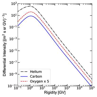
Figure 1.— The local interstellar spectra of CR helium (black dash-dotted line), carbon (blue solid line), and oxygen (red dashed line) as derived from the MCMC procedure (see text). Oxygen LIS is multiplied by a factor of 5 to avoid overlapping with carbon LIS.

3. Interstellar propagation

The LIS of CR species shown in Figure 1 are obtained using the optimization procedure employing GALPROP and HelMod codes in concert. The combined framework, described by Boschini et al. (2017b), is logically divided into two parts: i) a MCMC interface to version 56 of GALPROP (Masi, 2016), that enables the sampling of the CR production and propagation parameters space, and ii) an iterative procedure that, starting from GALPROP output, provides modulated spectra computed with HelMod to compare with AMS-02 data as observational constraints (Boschini et al., 2017a). The final product is a set of Galactic and heliospheric propagation parameters for all CR species that provides LIS that best reproduce available experimental data.

The basic features of CR propagation in the Galaxy are well-known, but the exact values of propagation parameters depend on the assumed propagation model and accuracy of selected CR datasets. Therefore, the MCMC procedure is employed to determine the propagation parameters using the best available CR measurements. Five main propagation parameters, that affect the overall shape of CR spectra, were left free in the scan using GALPROP running in the 2D mode: the Galactic halo half-width $z_{h}$, the normalization of the diffusion coefficient $D_{0}$ and the index of its rigidity dependence $\delta$, the Alfvén velocity $V_{\rm Alf}$, and the gradient of the convection velocity $dV_{\rm conv}/dz$ ($V_{\rm conv}=0$ in the plane, $z=0$). The radial size of the Galaxy does not significantly affect the values of propagation parameters and was set to 20 kpc. In addition, a factor $\beta^{\eta}$ is included in the diffusion coefficient, where $\beta=v/c$ and $\eta$ was left free. The best-fit value of $\eta=0.71$ improves the agreement at low energies, and slightly affects the choice of injection indices ${\gamma}_{0}$ an ${\gamma}_{1}$ (Table 2).

Inclusion of both distributed reacceleration and convection simultaneously is necessary to describe the high precision AMS-02 data, particularly in the range below 10 GV where their effects on CR spectra are significant (see Boschini et al., 2017b, for more details). The best-fit values of the main propagation parameters tuned to AMS-02 data are listed in Table 1, which are similar to those obtained by Boschini et al. (2017b) within the quoted error bars. The most significant change is a slight increase of the Alfvén velocity $V_{\rm Alf}$ by 2.4 km s^-1 which improves the agreement with the B/C ratio and electron data (Boschini et al., 2018).

The MCMC procedure is used only in the first step to define a consistent parameter space, then a methodical calibration of the model employing the HelMod module is performed. This procedure is described in detail in Section 3 of Boschini et al. (2017b), pp. 7, 8. Parameters of the injection spectra at low energies, such as spectral indices $\gamma_{i}(i=0,1,2)$ and the break rigidities $R_{i}(i=0,1)$, are left free in the procedure at this stage because their exact values depend on the solar modulation. Hence the low energy parts of the injection spectra are tuned together with the solar modulation parameters within their physical ranges in order to find best-fit solutions for all the observables. Consequently, the final values are coming from the GALPROP-HelMod combined fine-tuning, which involves an exploration of the parameter space around the best values defined in the first step.

Table 1Best-fit propagation parameters

N	Parameter		Best Value
1	$z_{h}$,	kpc	$4.0\pm 0.7$
2	$D_{0}$,	$10^{28}$ cm2 s-1	$4.3\pm 0.6$
3	$\delta$		$0.415\pm 0.025$
4	$V_{\rm Alf}$,	km s-1	$31\pm 3$
5	$dV_{\rm conv}/dz$,	km s-1 kpc-1	$9.8\pm 0.7$

Table 2Spectral parameters for CR species

Parameters	He	C	O	Error	$s_{i}$
$R_{0}$	$\cdots$	1 GV	1 GV	0.5	$-0.15$
$R_{1}$	7 GV	7 GV	7 GV	1	$-0.20$
$R_{2}$	325 GV	345 GV	360 GV	15	0.15
${\gamma}_{0}$	$\cdots$	1	1.1	0.06	$\cdots$
${\gamma}_{1}$	1.76	1.98	1.99	0.06	$\cdots$
${\gamma}_{2}$	2.39	2.42	2.46	0.04	$\cdots$
${\gamma}_{3}$	2.15	2.12	2.13	0.04	$\cdots$

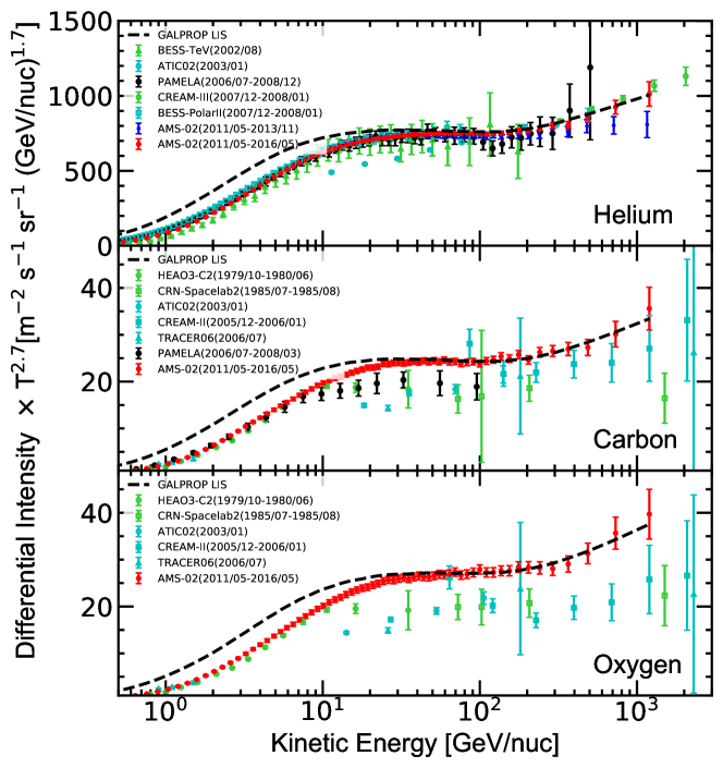
Figure 2.— The best fit helium LIS (top panel), carbon LIS (middle panel), and oxygen LIS (bottom panel) as a function of kinetic energy per nucleon shown together with the AMS-02 data (2011/05-2016/05, Aguilar et al., 2017), and previous measurements by ATIC (Panov et al., 2009), BESS (Shikaze et al., 2007; Abe et al., 2016), CREAM (Ahn et al., 2009; Yoon et al., 2017), HEAO3-C2 (Engelmann et al., 1990), CRN-Spacelab2 (Mueller et al., 1991), TRACER (Obermeier et al., 2011), and PAMELA (Adriani et al., 2011, 2014). Data points are taken from the LPSC Database of Charged Cosmic Rays (Maurin et al., 2014), and the corresponding experiments are listed in Table 3.

Table 3A list of high energy data used in this paper

Experiment	CR species	Reference	Experiment	CR species	Reference
HEAO3-C2 (1979/10-1980/06)	C, O	Engelmann et al. (1990)	PAMELA (2006/07-2008/03)	C	Adriani et al. (2014)
CRN-Spacelab2 (1985/07-1985/08)	C, O	Mueller et al. (1991)	PAMELA (2006/07-2008/12)	He	Adriani et al. (2011)
BESS-TeV (2002/08)	He	Shikaze et al. (2007)	CREAM-III (2007/12-2008/01)	He	Yoon et al. (2017)
ATIC02 (2003/01)	He, C, O	Panov et al. (2009)	BESS-PolarII (2007/12-2008/01)	He	Abe et al. (2016)
CREAM-II (2005/12-2006/01)	C, O	Ahn et al. (2009)	AMS-02 (2011/05-2013/11)	He	Aguilar et al. (2015a)
TRACER06 (2006/07)	C, O	Obermeier et al. (2011)	AMS-02 (2011/05-2016/05)	He, C, O	Aguilar et al. (2017)

In order to avoid sharp unphysical breaks in the LIS, we use the following parameterization for the source injection spectrum:

$$q(R)\propto\left(R/R_{0}\right)^{-\gamma_{0}}\prod_{i=0}^{2}\left[1+\left(R/R_{i}\right)^{\frac{\gamma_{i}-\gamma_{i+1}}{s_{i}}}\right]^{s_{i}},$$ (2)

where $s_{i}$ are the smoothing parameters, $s_{i}\lessgtr 0$ if $|\gamma_{i}|\lessgtr|\gamma_{i+1}|$. The values of $s_{i}(i=0,1,2)$ used in the fits are provided in Table 2.

Reproduction of the spectra of primary nuclei from MeV to TeV energies altogether requires an injection spectrum with three breaks. The MCMC scans in $\gamma_{i}$ and $R_{i}$ used the AMS-02 (Aguilar et al., 2017) and Voyager 1 (Cummings et al., 2016) data as constraints. At the following step, these parameters were slightly modified together with parameters of the solar modulation in order to find the best-fit solution for the LIS, as explained by Boschini et al. (2017b). Reproduction of the low-energy LIS corresponding to the direct measurements by Voyager 1 requires a break $R_{0}$ at 1 GV. The resulting best-fit spectral parameters are shown in Table 2.

The present analysis extends the dataset used in Boschini et al. (2017b) by including the newest published AMS-02 spectra of helium, carbon and oxygen that are based on the data collected during its first 5 years of operations (Aguilar et al., 2017). These measurements represent the current state-of-art knowledge of spectra of CR nuclei at high energies. In particular, it has been shown that the measured He-C-O spectra have a very similar rigidity dependence above 60 GV. They all deviate from a single power law above 200 GV and exhibit the same degree of spectral hardening (Aguilar et al., 2017). This spectral hardening is discussed in details in Section 4. The updated set of helium data (Figure 2, top panel) motivates the fine tuning of the injection spectral index $\gamma_{3}$ above the high-energy break with respect to the previous analysis of helium data that was based on the three years AMS-02 dataset. The new value is listed in Table 2. The helium LIS below 325 GV remains unchanged, and so do the modulated spectra, and is the same as published by Boschini et al. (2017b), therefore, it is not discussed further in this paper.

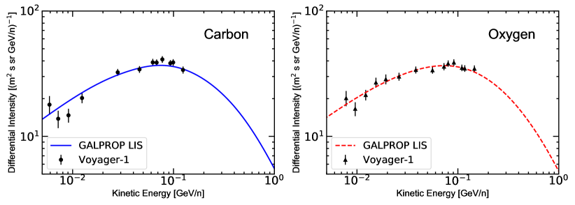
Figure 3.— A comparison of our best-set LIS (lines) with Voyager 1 2012-2015 monthly averaged data (points) shown as a function of kinetic energy per nucleon. Left panel: carbon spectrum, right panel: oxygen spectrum.

3.1. LIS of primary nuclei – direct observations

Accurate direct measurements of LIS are now available for several species at both low and high energies, and more is expected in coming years. Spectra of CR species above 100 GV are not affected by the heliospheric modulation and their measurements provide a direct probe of the LIS as discussed in details in Section 4. At low energies, from the second half of 2012, the Voyager 1 probe has been exploring the heliospheric boundaries providing invaluable data on the spectra of CR species in this region (Stone et al., 2013; Cummings et al., 2016). It is commonly accepted that Voyager 1 has been measuring the low-energy Galactic CRs from the local interstellar medium since that time (Krimigis et al., 2013; Gloeckler & Fisk, 2014).

The low-energy parameters of the injection spectra $\gamma_{0}$ and $R_{0}$ in the GALPROP runs were tuned using Voyager 1 data as constraints for the MCMC scans. Moreover, their fine tuning was performed simultaneously with fine tuning of the solar modulation parameters (through the procedure described in Section 2.2) in order to find the best-fit solution, using the same procedure as described by Boschini et al. (2017b). In Figure 3 the carbon and oxygen LIS are compared with their average intensities measured from the end of 2012 to the middle of 2015 (Cummings et al., 2016). The presented model provides a good description of the LIS at low energies. The resulting best-fit spectral parameters are listed in Table 2 and remain the baseline solution for all scenarios discussed in this paper.

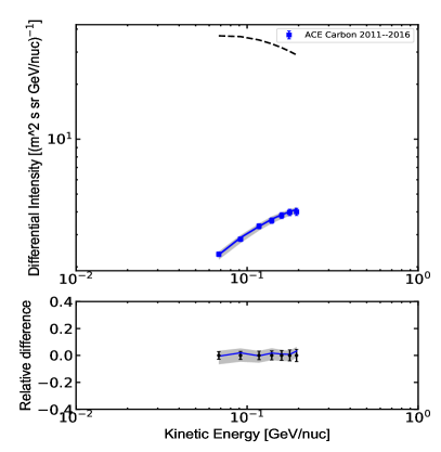
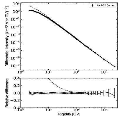
Figure 4.— Differential intensity of CR carbon, left panel: ACE/CRIS, right panel: AMS-02. Points represent experimental data, dashed line is the GALPROP LIS, and solid line shows the computed modulated spectrum. The bottom panels show the relative difference between the modulated spectrum and experimental data. Data are presented in units of kinetic energy per nucleon or rigidity – dependently on the experimental technique.

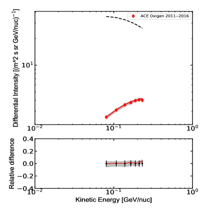
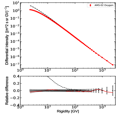
Figure 5.— Differential intensity of CR oxygen, left panel: ACE/CRIS, right panel: AMS-02. The bottom panels show the relative difference between the modulated spectrum and experimental data. Line coding is the same as in Figure 4.

At high energies, where the CR spectra are not affected by the heliospheric modulation, AMS-02 data are used up to $\sim$2 TV, and further extension of the rigidity range to 20–30 TV is possible using high energy measurements (Table 3) available from the LPSC Database of Charged Cosmic Rays (Maurin et al., 2014). More details are given in Section 4.

3.2. The modulated spectrum: Data at Earth

Direct CR measurements that are made deep in the heliosphere, e.g., near the Earth, are affected by the solar modulation and cannot be compared directly to the LIS. Therefore, the HelMod code (Boschini et al., 2017b) is used to calculate the modulated spectra of CR carbon and oxygen. The HelMod code, described in Section 2.2, was tuned to provide the same level of accuracy at any level of solar activity, high and low, and for all kinds of isotopes ($Z/A$) propagating in the heliosphere using the same set of basic parameters (see Boschini et al., 2017a, for more details).

In this paper the modulated spectra of carbon and oxygen are compared with appropriate measurements by ACE/CRIS (George et al., 2009), AMS-02 (Aguilar et al., 2017), HEAO-3 (Engelmann et al., 1990), and PAMELA (Adriani et al., 2014). Figures 4 and 5 show the calculated spectra compared with ACE/CRIS and AMS-02 data. The calculated spectra are integrated over the time period corresponding to the AMS-02 data taking (from May 2011 to May 2016), where the quoted error bars include both statistical and systematic uncertainties.

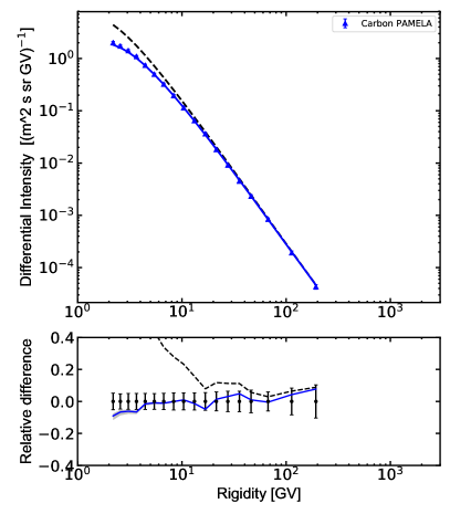
Figure 6.— Differential intensity of carbon from PAMELA experiment. Line coding is the same as in Figure 4. The GALPROP LIS is multiplied by 0.85 (dashed line) to match the experimental data.

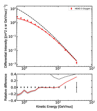
Figure 7.— Differential intensity of carbon from HEAO-3 experiment. Line coding is the same as in Figure 4.

In Figure 6 the modulated spectrum is compared with the PAMELA data taken during the period of the solar minimum spanning from July 2006 to March 2008. The GALPROP LIS is multiplied by 0.85 to match the experimental data. We do not speculate about the origin of this factor, but point out that it may be connected with the evaluation of the selection efficiency (see footnote 24 in Adriani et al., 2013). Figure 7 shows a comparison with HEAO-3 data collected from Oct 1979 to June 1980. To reproduce the proper time span for each experiment, the HelMod modulated spectra were evaluated for each Carrington rotation during the period of observations, and then the results were used to evaluate a unique normalized probability function for the modulation tool as described in Section 3.1 of Boschini et al. (2017b).

Note that the AMS-02 measurements of the carbon spectrum (Aguilar et al., 2017) are distinctly different from the results of the previous experiments, which show 20–25% lower intensity above 20 GV (see Figure 2). The discrepancy is even larger for oxygen (same Figure). Therefore, in this paper, for each presented dataset, a normalization factor that rescales the LIS to the published values is calculated, while AMS-02 data are used for the described MCMC procedure due to the small systematic and statistical uncertainties. The renormalized spectra generally agree well with the available data, but some discrepancies with earlier experiments remain (Figure 7).

4. High Energy spectrum

Direct measurements of primary CR species and detection of their spectral features may be able to provide a hint at the origin and properties of CR acceleration sites and/or properties of the interstellar medium. Unexpected flattening and breaks in the spectra of CR protons, helium, and heavier nuclei observed by ATIC (Panov et al., 2009), CREAM (Ahn et al., 2010; Yoon et al., 2011), PAMELA (Adriani et al., 2011), and more recently by AMS-02 (Aguilar et al., 2015b, a, 2017), that can be seen in Figure 2, stimulated a rich discussion of the origin of high-energy hardening in the spectra of CR species (see, e.g., Vladimirov et al., 2012; Bernard et al., 2013; Tomassetti, 2015; Ohira et al., 2016). AMS-02 measurements indicate that the values of the spectral indices of carbon and oxygen with high precision resemble the value of the helium index (see Figure 8 and 9). This supports the idea that the primary species are likely accelerated in the same processes or/and sources. In this scenario the break at high energies may be the intrinsic property of the sources or of the acceleration mechanism itself, thus requiring an ad hoc break in the injection spectra.

Table 4Parameters of the analytical fits to the carbon and oxygen LIS

Carbon, $R_{d}=2$ GV						Oxygen, $R_{d}=2$ GV
$a_{0}=$	0.33318	$p_{-2}=$	6.864	$g_{1}=$	0	$a_{0}=$	0	$p_{-2}=$	0	$g_{1}=$	6910
$a_{1}=$	–28.356	$p_{-1}=$	–16.169	$h_{1}=$	0	$a_{1}=$	0	$p_{-1}=$	0	$h_{1}=$	134.86
$a_{2}=$	40.530	$p_{0}=$	40.68	$l_{1}=$	0	$a_{2}=$	–8.7059	$p_{0}=$	146.19	$l_{1}=$	1.3348
$a_{3}=$	–8.8178	$p_{1}=$	–0.0098494	$g_{2}=$	0	$a_{3}=$	28.64	$p_{1}=$	0.0023718	$g_{2}=$	–10698.7
$a_{4}=$	0	$p_{2}=$	1.992$\times 10^{-7}$	$h_{2}=$	0	$a_{4}=$	–13.92	$p_{2}=$	0	$h_{2}=$	130.448
$a_{5}=$	0	$f=$	1.7727	$l_{2}=$	0	$a_{5}=$	2.03539	$f=$	0	$l_{2}=$	0.0879
$b=$	686.15	$g_{0}=$	4989	$m=$	–515.22	$b=$	0	$g_{0}=$	–224.146	$m=$	0
$c=$	31.045	$h_{0}=$	86.075	$n=$	5.2815	$c=$	0	$h_{0}=$	0.920357	$n=$	0
$d=$	127.83	$l_{0}=$	1	$o=$	1	$d=$	0	$l_{0}=$	1	$o=$	0

Another reasonable hypothesis is to assume a change in the slope of the diffusion coefficient around 350 GV (Vladimirov et al., 2012) that would affect all CR species whose spectra and breaks will be aligned automatically. As discussed by Boschini et al. (2017b), the flattening of helium, carbon, and oxygen spectra is then reproduced if the index of the rigidity dependence of the diffusion coefficient $\delta$ is reduced above the break rigidity by $\Delta\delta\approx 0.27$. In the framework of the model discussed in this paper that means changing $\delta$ from 0.415 to $\sim$0.15. However, the discrimination of the two scenarios cannot be made without accurate measurements of secondary nuclei. A forthcoming paper will report on the analysis of the secondary species, which is currently underway. This subsequent work takes advantage of the just-published AMS-02 observations of CR lithium, beryllium, and boron (Aguilar et al., 2018).

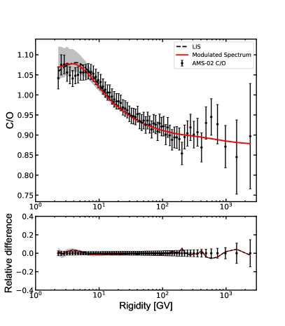
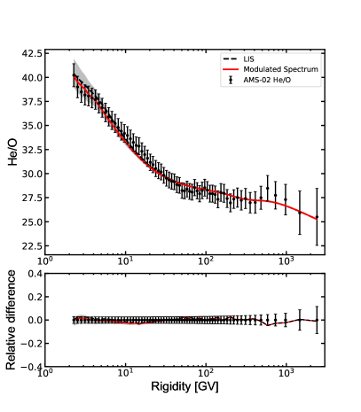
Figure 8.— The carbon/oxygen (left) and helium/oxygen (right) ratios as measured by AMS-02 are compared with calculated ratios for LIS (dashed line) and modulated ratios (red line).

In addition to the plots and the tabulated data presented in Section 3.2 and Appendix Supplementary Material, the analytical expression is provided for the GALPROP LIS, from 3 MV up to 10 TV:

$$F(R)\times R^{2.7}=$$ (3)

$$\left\{\begin{array}[]{ll}\sum_{i=0}^{5}a_{i}R^{i}+\frac{bR}{c+dR^{2}},&R\leq R_{d},\vskip 3.0pt plus 1.0pt minus 1.0pt\\ \sum_{i=-2}^{2}p_{i}R^{i}\!+\!f\sqrt{R}\!+\!\sum_{i=0}^{2}\frac{g_{i}}{h_{i}+l_{i}R}\!+\!\frac{m}{n+oR^{2}},&R>R_{d},\end{array}\right.$$

where $a_{i},b,c,d,e,f,g_{i},h_{i},l_{i},m,n,o,p_{i}$ are the numerical coefficients summarized in Table 4, and $R$ is the rigidity in GV. The fit is tuned to agree with Voyager 1 measurements at low rigidities and matches the GALPROP-calculated LIS in the energy range where no data points are available. The derived expressions are virtually identical, within 1%–5%, to numerical solutions spanning over 5 orders of magnitude in rigidity, including the spectral flattening at high energies. The search for the analytic solutions – using the same algorithm of Boschini et al. (2017b) – was guided by the advanced MCMC fitting procedure such as Eureqa.

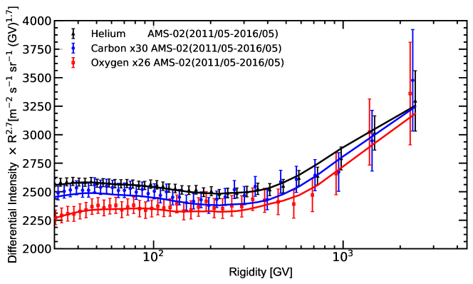
Figure 9.— The AMS-02 measurements of helium (black triangles), carbon (blue points), and oxygen (red squares) are compared with the corresponding GALPROP-LIS modulated with HelMod (solid lines).

5. Summary

The helium, carbon, and oxygen LIS derived in the current work provide a good description of the Voyager 1, ACE/CRIS, HEAO-3, PAMELA, and AMS-02 data over the energy range from MeV/n to tens of TeV/n. The work presented in this paper demonstrates that the CR data collected during the solar cycles 23 and 24 can be successfully reproduced within a single framework. This includes a fully realistic and exhaustive description of the relevant CR physics. Given their high precision, recent AMS-02 data can be used to put useful constraints of processes of particle acceleration, CR sources, properties of the interstellar medium, search for signatures of dark matter, and many others. This work complements earlier results on the proton, He, antiproton, and electron LIS illustrating a significant potential of the combined GALPROP-HelMod framework.

Supplementary Material

Table 5Carbon LIS

Rigidity	Differential	Rigidity	Differential	Rigidity	Differential	Rigidity	Differential	Rigidity	Differential
GV	Intensity	GV	Intensity	GV	Intensity	GV	Intensity	GV	Intensity
Rigidity Differential Rigidity Differential Rigidity Differential Rigidity Differential Rigidity Differential GV Intensity GV Intensity GV Intensity GV Intensity GV Intensity Rigidity Differential Rigidity Differential Rigidity Differential Rigidity Differential Rigidity Differential GV Intensity GV Intensity GV Intensity GV Intensity GV Intensity 9.354e-02 1.412e-01 5.922e-01 5.255e+00 4.965e+00 1.048e+00 1.425e+02 1.262e-04 5.518e+03 9.869e-09 9.678e-02 1.526e-01 6.131e-01 5.489e+00 5.218e+00 9.316e-01 1.523e+02 1.049e-04 5.906e+03 8.318e-09 1.001e-01 1.647e-01 6.348e-01 5.724e+00 5.487e+00 8.262e-01 1.629e+02 8.720e-05 6.321e+03 7.010e-09 1.036e-01 1.778e-01 6.573e-01 5.959e+00 5.773e+00 7.308e-01 1.742e+02 7.251e-05 6.765e+03 5.908e-09 1.072e-01 1.919e-01 6.806e-01 6.192e+00 6.077e+00 6.450e-01 1.863e+02 6.032e-05 7.241e+03 4.979e-09 1.109e-01 2.071e-01 7.048e-01 6.420e+00 6.402e+00 5.679e-01 1.993e+02 5.019e-05 7.750e+03 4.196e-09 1.147e-01 2.235e-01 7.299e-01 6.641e+00 6.747e+00 4.988e-01 2.132e+02 4.177e-05 8.295e+03 3.536e-09 1.187e-01 2.411e-01 7.560e-01 6.854e+00 7.115e+00 4.371e-01 2.280e+02 3.479e-05 8.879e+03 2.980e-09 1.228e-01 2.601e-01 7.830e-01 7.056e+00 7.507e+00 3.821e-01 2.439e+02 2.898e-05 9.503e+03 2.511e-09 1.270e-01 2.806e-01 8.111e-01 7.246e+00 7.926e+00 3.332e-01 2.610e+02 2.416e-05 1.017e+04 2.116e-09 1.314e-01 3.027e-01 8.402e-01 7.422e+00 8.372e+00 2.898e-01 2.792e+02 2.014e-05 1.089e+04 1.783e-09 1.360e-01 3.264e-01 8.705e-01 7.583e+00 8.849e+00 2.514e-01 2.987e+02 1.681e-05 1.165e+04 1.502e-09 1.407e-01 3.519e-01 9.019e-01 7.726e+00 9.357e+00 2.176e-01 3.195e+02 1.403e-05 1.247e+04 1.266e-09 1.456e-01 3.794e-01 9.346e-01 7.849e+00 9.900e+00 1.880e-01 3.419e+02 1.172e-05 1.335e+04 1.066e-09 1.506e-01 4.089e-01 9.685e-01 7.953e+00 1.048e+01 1.620e-01 3.658e+02 9.800e-06 1.429e+04 8.986e-10 1.558e-01 4.407e-01 1.004e+00 8.036e+00 1.110e+01 1.394e-01 3.914e+02 8.197e-06 1.529e+04 7.571e-10 1.612e-01 4.748e-01 1.041e+00 8.098e+00 1.176e+01 1.197e-01 4.187e+02 6.860e-06 1.637e+04 6.378e-10 1.668e-01 5.114e-01 1.079e+00 8.137e+00 1.247e+01 1.025e-01 4.480e+02 5.745e-06 1.752e+04 5.374e-10 1.726e-01 5.506e-01 1.119e+00 8.154e+00 1.322e+01 8.764e-02 4.794e+02 4.815e-06 1.875e+04 4.527e-10 1.785e-01 5.928e-01 1.160e+00 8.148e+00 1.403e+01 7.479e-02 5.130e+02 4.037e-06 2.007e+04 3.814e-10 1.847e-01 6.379e-01 1.203e+00 8.120e+00 1.489e+01 6.372e-02 5.489e+02 3.387e-06 2.148e+04 3.213e-10 1.911e-01 6.863e-01 1.248e+00 8.070e+00 1.582e+01 5.419e-02 5.874e+02 2.843e-06 2.299e+04 2.707e-10 1.978e-01 7.382e-01 1.295e+00 7.998e+00 1.680e+01 4.602e-02 6.286e+02 2.387e-06 2.461e+04 2.280e-10 2.046e-01 7.936e-01 1.343e+00 7.904e+00 1.786e+01 3.903e-02 6.727e+02 2.006e-06 2.634e+04 1.921e-10 2.117e-01 8.530e-01 1.394e+00 7.789e+00 1.899e+01 3.305e-02 7.198e+02 1.686e-06 2.819e+04 1.618e-10 2.190e-01 9.164e-01 1.448e+00 7.653e+00 2.020e+01 2.794e-02 7.703e+02 1.417e-06 3.017e+04 1.363e-10 2.266e-01 9.841e-01 1.503e+00 7.497e+00 2.149e+01 2.360e-02 8.243e+02 1.192e-06 3.230e+04 1.148e-10 2.345e-01 1.056e+00 1.561e+00 7.321e+00 2.287e+01 1.990e-02 8.822e+02 1.003e-06 3.457e+04 9.671e-11 2.426e-01 1.133e+00 1.622e+00 7.127e+00 2.435e+01 1.676e-02 9.441e+02 8.441e-07 3.700e+04 8.146e-11 2.511e-01 1.215e+00 1.685e+00 6.916e+00 2.593e+01 1.410e-02 1.010e+03 7.105e-07 3.960e+04 6.862e-11 2.598e-01 1.303e+00 1.751e+00 6.689e+00 2.762e+01 1.185e-02 1.081e+03 5.983e-07 4.239e+04 5.780e-11 2.688e-01 1.395e+00 1.821e+00 6.448e+00 2.943e+01 9.947e-03 1.157e+03 5.039e-07 4.537e+04 4.868e-11 2.781e-01 1.494e+00 1.893e+00 6.194e+00 3.137e+01 8.343e-03 1.238e+03 4.245e-07 4.856e+04 4.100e-11 2.878e-01 1.599e+00 1.969e+00 5.927e+00 3.344e+01 6.991e-03 1.325e+03 3.576e-07 5.197e+04 3.453e-11 2.978e-01 1.709e+00 2.049e+00 5.651e+00 3.566e+01 5.854e-03 1.418e+03 3.013e-07 5.563e+04 2.909e-11 3.081e-01 1.826e+00 2.133e+00 5.367e+00 3.803e+01 4.898e-03 1.518e+03 2.539e-07 5.954e+04 2.450e-11 3.189e-01 1.949e+00 2.221e+00 5.079e+00 4.057e+01 4.096e-03 1.625e+03 2.139e-07 6.373e+04 2.063e-11 3.300e-01 2.079e+00 2.314e+00 4.788e+00 4.329e+01 3.422e-03 1.739e+03 1.803e-07 6.821e+04 1.738e-11 3.414e-01 2.215e+00 2.411e+00 4.498e+00 4.620e+01 2.858e-03 1.861e+03 1.520e-07 7.301e+04 1.464e-11 3.533e-01 2.358e+00 2.514e+00 4.210e+00 4.932e+01 2.385e-03 1.992e+03 1.281e-07 7.814e+04 1.233e-11 3.656e-01 2.507e+00 2.622e+00 3.926e+00 5.265e+01 1.989e-03 2.132e+03 1.080e-07 8.364e+04 1.038e-11 3.784e-01 2.663e+00 2.735e+00 3.649e+00 5.621e+01 1.659e-03 2.282e+03 9.100e-08 8.952e+04 8.743e-12 3.916e-01 2.826e+00 2.855e+00 3.380e+00 6.003e+01 1.382e-03 2.442e+03 7.671e-08 9.582e+04 7.363e-12 4.053e-01 2.995e+00 2.981e+00 3.120e+00 6.412e+01 1.151e-03 2.613e+03 6.467e-08 1.026e+05 6.201e-12 4.194e-01 3.170e+00 3.115e+00 2.871e+00 6.849e+01 9.589e-04 2.797e+03 5.451e-08 1.098e+05 5.222e-12 4.341e-01 3.352e+00 3.256e+00 2.633e+00 7.317e+01 7.982e-04 2.994e+03 4.595e-08 1.175e+05 4.398e-12 4.493e-01 3.539e+00 3.405e+00 2.407e+00 7.817e+01 6.643e-04 3.204e+03 3.874e-08 1.258e+05 3.703e-12 4.650e-01 3.733e+00 3.563e+00 2.193e+00 8.353e+01 5.527e-04 3.429e+03 3.265e-08 1.346e+05 3.119e-12 4.813e-01 3.934e+00 3.730e+00 1.992e+00 8.927e+01 4.597e-04 3.670e+03 2.752e-08 1.441e+05 2.626e-12 4.982e-01 4.140e+00 3.906e+00 1.804e+00 9.541e+01 3.823e-04 3.928e+03 2.320e-08 1.542e+05 2.212e-12 5.156e-01 4.353e+00 4.094e+00 1.628e+00 1.020e+02 3.179e-04 4.205e+03 1.956e-08 1.650e+05 1.862e-12 5.338e-01 4.571e+00 4.293e+00 1.465e+00 1.090e+02 2.643e-04 4.500e+03 1.648e-08 1.767e+05 1.569e-12 5.526e-01 4.795e+00 4.503e+00 1.314e+00 1.165e+02 2.197e-04 4.817e+03 1.389e-08 1.891e+05 1.317e-12 5.720e-01 5.023e+00 4.727e+00 1.175e+00 1.246e+02 1.826e-04 5.155e+03 1.171e-08 2.024e+05 1.054e-12

Table 6Oxygen LIS

Rigidity	Differential	Rigidity	Differential	Rigidity	Differential	Rigidity	Differential	Rigidity	Differential
GV	Intensity	GV	Intensity	GV	Intensity	GV	Intensity	GV	Intensity
Rigidity Differential Rigidity Differential Rigidity Differential Rigidity Differential Rigidity Differential GV Intensity GV Intensity GV Intensity GV Intensity GV Intensity 9.714e-02 1.655e-01 6.150e-01 5.553e+00 5.156e+00 9.070e-01 1.479e+02 1.266e-04 5.730e+03 1.025e-08 1.005e-01 1.784e-01 6.367e-01 5.784e+00 5.419e+00 8.073e-01 1.582e+02 1.054e-04 6.133e+03 8.641e-09 1.040e-01 1.922e-01 6.592e-01 6.014e+00 5.698e+00 7.172e-01 1.692e+02 8.768e-05 6.564e+03 7.281e-09 1.076e-01 2.071e-01 6.826e-01 6.241e+00 5.995e+00 6.359e-01 1.809e+02 7.298e-05 7.026e+03 6.135e-09 1.113e-01 2.231e-01 7.068e-01 6.463e+00 6.311e+00 5.626e-01 1.935e+02 6.076e-05 7.520e+03 5.169e-09 1.151e-01 2.404e-01 7.319e-01 6.680e+00 6.648e+00 4.968e-01 2.070e+02 5.060e-05 8.048e+03 4.355e-09 1.191e-01 2.589e-01 7.580e-01 6.889e+00 7.006e+00 4.377e-01 2.214e+02 4.216e-05 8.614e+03 3.669e-09 1.233e-01 2.789e-01 7.850e-01 7.087e+00 7.389e+00 3.848e-01 2.368e+02 3.513e-05 9.220e+03 3.091e-09 1.275e-01 3.003e-01 8.131e-01 7.274e+00 7.796e+00 3.375e-01 2.533e+02 2.929e-05 9.868e+03 2.604e-09 1.319e-01 3.234e-01 8.423e-01 7.448e+00 8.231e+00 2.953e-01 2.710e+02 2.444e-05 1.056e+04 2.194e-09 1.365e-01 3.481e-01 8.725e-01 7.606e+00 8.694e+00 2.578e-01 2.899e+02 2.040e-05 1.131e+04 1.848e-09 1.412e-01 3.747e-01 9.039e-01 7.748e+00 9.189e+00 2.246e-01 3.102e+02 1.703e-05 1.210e+04 1.556e-09 1.461e-01 4.033e-01 9.366e-01 7.871e+00 9.717e+00 1.953e-01 3.318e+02 1.423e-05 1.295e+04 1.311e-09 1.512e-01 4.339e-01 9.705e-01 7.975e+00 1.028e+01 1.694e-01 3.550e+02 1.190e-05 1.386e+04 1.104e-09 1.564e-01 4.668e-01 1.006e+00 8.057e+00 1.088e+01 1.467e-01 3.798e+02 9.959e-06 1.484e+04 9.298e-10 1.618e-01 5.020e-01 1.042e+00 8.118e+00 1.153e+01 1.267e-01 4.064e+02 8.338e-06 1.588e+04 7.831e-10 1.674e-01 5.398e-01 1.081e+00 8.156e+00 1.221e+01 1.092e-01 4.348e+02 6.986e-06 1.700e+04 6.595e-10 1.732e-01 5.803e-01 1.120e+00 8.169e+00 1.295e+01 9.398e-02 4.653e+02 5.857e-06 1.819e+04 5.553e-10 1.792e-01 6.237e-01 1.162e+00 8.159e+00 1.373e+01 8.070e-02 4.979e+02 4.913e-06 1.947e+04 4.676e-10 1.854e-01 6.700e-01 1.205e+00 8.124e+00 1.457e+01 6.916e-02 5.327e+02 4.124e-06 2.084e+04 3.938e-10 1.918e-01 7.196e-01 1.249e+00 8.063e+00 1.547e+01 5.916e-02 5.701e+02 3.463e-06 2.231e+04 3.315e-10 1.985e-01 7.727e-01 1.296e+00 7.979e+00 1.643e+01 5.051e-02 6.100e+02 2.910e-06 2.388e+04 2.792e-10 2.054e-01 8.293e-01 1.344e+00 7.870e+00 1.745e+01 4.305e-02 6.528e+02 2.446e-06 2.555e+04 2.350e-10 2.125e-01 8.898e-01 1.395e+00 7.737e+00 1.855e+01 3.663e-02 6.985e+02 2.057e-06 2.735e+04 1.979e-10 2.198e-01 9.543e-01 1.448e+00 7.583e+00 1.972e+01 3.112e-02 7.475e+02 1.731e-06 2.928e+04 1.666e-10 2.275e-01 1.023e+00 1.503e+00 7.409e+00 2.097e+01 2.640e-02 7.999e+02 1.457e-06 3.133e+04 1.403e-10 2.354e-01 1.096e+00 1.561e+00 7.215e+00 2.231e+01 2.236e-02 8.561e+02 1.226e-06 3.354e+04 1.181e-10 2.435e-01 1.174e+00 1.621e+00 7.003e+00 2.375e+01 1.891e-02 9.161e+02 1.033e-06 3.590e+04 9.940e-11 2.520e-01 1.257e+00 1.684e+00 6.774e+00 2.528e+01 1.598e-02 9.804e+02 8.699e-07 3.842e+04 8.367e-11 2.607e-01 1.345e+00 1.750e+00 6.531e+00 2.693e+01 1.348e-02 1.049e+03 7.330e-07 4.112e+04 7.043e-11 2.698e-01 1.438e+00 1.819e+00 6.275e+00 2.868e+01 1.136e-02 1.123e+03 6.177e-07 4.402e+04 5.929e-11 2.791e-01 1.537e+00 1.891e+00 6.009e+00 3.056e+01 9.565e-03 1.202e+03 5.206e-07 4.711e+04 4.990e-11 2.888e-01 1.641e+00 1.966e+00 5.736e+00 3.258e+01 8.045e-03 1.286e+03 4.388e-07 5.043e+04 4.200e-11 2.989e-01 1.752e+00 2.045e+00 5.456e+00 3.473e+01 6.760e-03 1.376e+03 3.699e-07 5.397e+04 3.536e-11 3.092e-01 1.869e+00 2.128e+00 5.173e+00 3.703e+01 5.675e-03 1.473e+03 3.118e-07 5.777e+04 2.976e-11 3.200e-01 1.992e+00 2.215e+00 4.889e+00 3.950e+01 4.761e-03 1.576e+03 2.629e-07 6.183e+04 2.505e-11 3.311e-01 2.121e+00 2.307e+00 4.606e+00 4.213e+01 3.990e-03 1.687e+03 2.216e-07 6.618e+04 2.108e-11 3.426e-01 2.257e+00 2.403e+00 4.324e+00 4.496e+01 3.342e-03 1.806e+03 1.869e-07 7.083e+04 1.774e-11 3.546e-01 2.400e+00 2.504e+00 4.045e+00 4.798e+01 2.796e-03 1.933e+03 1.575e-07 7.582e+04 1.493e-11 3.669e-01 2.550e+00 2.610e+00 3.770e+00 5.121e+01 2.339e-03 2.068e+03 1.328e-07 8.115e+04 1.256e-11 3.797e-01 2.707e+00 2.722e+00 3.502e+00 5.467e+01 1.955e-03 2.214e+03 1.120e-07 8.686e+04 1.057e-11 3.929e-01 2.871e+00 2.840e+00 3.242e+00 5.838e+01 1.633e-03 2.369e+03 9.446e-08 9.296e+04 8.898e-12 4.066e-01 3.042e+00 2.965e+00 2.993e+00 6.234e+01 1.363e-03 2.536e+03 7.965e-08 9.950e+04 7.488e-12 4.208e-01 3.220e+00 3.096e+00 2.754e+00 6.658e+01 1.137e-03 2.714e+03 6.715e-08 1.065e+05 6.301e-12 4.355e-01 3.405e+00 3.235e+00 2.526e+00 7.112e+01 9.487e-04 2.905e+03 5.662e-08 1.140e+05 5.302e-12 4.508e-01 3.597e+00 3.381e+00 2.310e+00 7.598e+01 7.910e-04 3.109e+03 4.774e-08 1.220e+05 4.462e-12 4.665e-01 3.795e+00 3.536e+00 2.106e+00 8.118e+01 6.593e-04 3.327e+03 4.025e-08 1.306e+05 3.755e-12 4.829e-01 3.999e+00 3.700e+00 1.914e+00 8.675e+01 5.493e-04 3.561e+03 3.393e-08 1.398e+05 3.159e-12 4.998e-01 4.208e+00 3.873e+00 1.734e+00 9.270e+01 4.575e-04 3.812e+03 2.860e-08 1.496e+05 2.658e-12 5.173e-01 4.423e+00 4.057e+00 1.567e+00 9.908e+01 3.810e-04 4.080e+03 2.411e-08 1.601e+05 2.237e-12 5.355e-01 4.643e+00 4.251e+00 1.412e+00 1.059e+02 3.172e-04 4.366e+03 2.032e-08 1.714e+05 1.882e-12 5.543e-01 4.867e+00 4.458e+00 1.268e+00 1.132e+02 2.640e-04 4.673e+03 1.713e-08 1.834e+05 1.584e-12 5.738e-01 5.093e+00 4.677e+00 1.137e+00 1.210e+02 2.197e-04 5.002e+03 1.444e-08 1.963e+05 1.306e-12 5.940e-01 5.323e+00 4.909e+00 1.017e+00 1.294e+02 1.828e-04 5.354e+03 1.217e-08 2.102e+05 9.688e-13

References

- Abe et al. (2016) Abe, K., Fuke, H., Haino, S., et al. 2016, ApJ, 822, 65
- Adriani et al. (2011) Adriani, O., Barbarino, G. C., Bazilevskaya, G. A., et al. 2011, Science, 332, 69
- Adriani et al. (2013) —. 2013, ApJ, 765, 91
- Adriani et al. (2014) —. 2014, ApJ, 791, 93
- Aguilar et al. (2013) Aguilar, M., Alberti, G., Alpat, B., et al. 2013, Physical Review Letters, 110, 141102
- Aguilar et al. (2015a) Aguilar, M., Aisa, D., Alpat, B., et al. 2015a, Physical Review Letters, 115, 211101
- Aguilar et al. (2015b) —. 2015b, Physical Review Letters, 114, 171103
- Aguilar et al. (2017) Aguilar, M., Ali Cavasonza, L., Alpat, B., et al. 2017, Physical Review Letters, 119, 251101
- Aguilar et al. (2018) Aguilar, M., Ali Cavasonza, L., Ambrosi, G., et al. 2018, Physical Review Letters, 120, 021101
- Ahn et al. (2009) Ahn, H. S., Allison, P., Bagliesi, M. G., et al. 2009, ApJ, 707, 593
- Ahn et al. (2010) —. 2010, ApJ, 714, L89
- Atwood et al. (2009) Atwood, W. B., Abdo, A. A., Ackermann, M., et al. 2009, ApJ, 697, 1071
- Bernard et al. (2013) Bernard, G., Delahaye, T., Keum, Y.-Y., et al. 2013, A&A, 555, A48
- Bobik et al. (2012) Bobik, P., Boella, G., Boschini, M. J., et al. 2012, ApJ, 745, 132
- Bobik et al. (2016) Bobik, P., Boschini, M. J., Della Torre, S., et al. 2016, Journal of Geophysical Research (Space Physics), 121, 3920
- Boschini et al. (2017a) Boschini, M. J., Della Torre, S., Gervasi, M., La Vacca, G., & Rancoita, P. G. 2017a, Adv. Space Res. In Press, Available online 27 April 2017, arXiv:1704.03733
- Boschini et al. (2017b) Boschini, M. J., Della Torre, S., Gervasi, M., et al. 2017b, ApJ, 840, 115
- Boschini et al. (2018) —. 2018, ApJ, 854, 94
- Cummings et al. (2016) Cummings, A. C., Stone, E. C., Heikkila, B. C., et al. 2016, ApJ, 831, 18
- Dialynas et al. (2017) Dialynas, K., Krimigis, S. M., Mitchell, D. G., Decker, R. B., & Roelof, E. C. 2017, Nature Astronomy, 1, 0115
- Engelbrecht et al. (2017) Engelbrecht, N. E., Strauss, R. D., le Roux, J. A., & Burger, R. A. 2017, ApJ, 841, 107
- Engelmann et al. (1990) Engelmann, J. J., Ferrando, P., Soutoul, A., Goret, P., & Juliusson, E. 1990, A&A, 233, 96
- George et al. (2009) George, J. S., Lave, K. A., Wiedenbeck, M. E., et al. 2009, ApJ, 698, 1666
- Gloeckler & Fisk (2014) Gloeckler, G., & Fisk, L. A. 2014, Geophys. Res. Lett., 41, 5325
- Jóhannesson et al. (2016) Jóhannesson, G., Ruiz de Austri, R., Vincent, A. C., et al. 2016, ApJ, 824, 16
- Krimigis et al. (2013) Krimigis, S. M., Decker, R. B., Roelof, E. C., et al. 2013, Science, 341, 144
- Masi (2016) Masi, N. 2016, Il Nuovo Cimento C, 39, 282
- Maurin et al. (2014) Maurin, D., Melot, F., & Taillet, R. 2014, A&A, 569, A32
- Moskalenko et al. (2015) Moskalenko, I. V., Jóhannesson, G., Orlando, E., et al. 2015, Proc. 34th ICRC (Hague), 492
- Moskalenko & Strong (1998) Moskalenko, I. V., & Strong, A. W. 1998, ApJ, 493, 694
- Moskalenko & Strong (2000) —. 2000, ApJ, 528, 357
- Moskalenko et al. (2003) Moskalenko, I. V., Strong, A. W., Mashnik, S. G., & Ormes, J. F. 2003, ApJ, 586, 1050
- Moskalenko et al. (2002) Moskalenko, I. V., Strong, A. W., Ormes, J. F., & Potgieter, M. S. 2002, ApJ, 565, 280
- Mueller et al. (1991) Mueller, D., Swordy, S. P., Meyer, P., L’Heureux, J., & Grunsfeld, J. M. 1991, ApJ, 374, 356
- Obermeier et al. (2011) Obermeier, A., Ave, M., Boyle, P., et al. 2011, ApJ, 742, 14
- Ohira et al. (2016) Ohira, Y., Kawanaka, N., & Ioka, K. 2016, Phys. Rev. D, 93, 083001
- Panov et al. (2009) Panov, A. D., Adams, J. H., Ahn, H. S., et al. 2009, Bulletin of the Russian Academy of Sciences, Physics, 73, 564
- Parker (1965) Parker, E. N. 1965, Planet. Space Sci., 13, 9
- Picozza et al. (2007) Picozza, P., Galper, A. M., Castellini, G., et al. 2007, Astroparticle Physics, 27, 296
- Porter et al. (2017) Porter, T. A., Jóhannesson, G., & Moskalenko, I. V. 2017, ApJ, 846, 67
- Ptuskin et al. (2006) Ptuskin, V. S., Moskalenko, I. V., Jones, F. C., Strong, A. W., & Zirakashvili, V. N. 2006, ApJ, 642, 902
- Scherer et al. (2011) Scherer, K., Fichtner, H., Strauss, R. D., et al. 2011, ApJ, 735, 128
- Shikaze et al. (2007) Shikaze, Y., Orito, S., Mitsui, T., & BESS Collaboration. 2007, Astrop. Phys., 28, 154
- Stone et al. (2013) Stone, E. C., Cummings, A. C., McDonald, F. B., et al. 2013, Science, 341, 150
- Strong & Moskalenko (1998) Strong, A. W., & Moskalenko, I. V. 1998, ApJ, 509, 212
- Strong et al. (2007) Strong, A. W., Moskalenko, I. V., & Ptuskin, V. S. 2007, Ann. Rev. Nucl. Part. Sci., 57, 285
- Strong et al. (2000) Strong, A. W., Moskalenko, I. V., & Reimer, O. 2000, ApJ, 537, 763
- Strong et al. (2004) —. 2004, ApJ, 613, 962
- Tomassetti (2015) Tomassetti, N. 2015, ApJ, 815, L1
- Trotta et al. (2011) Trotta, R., Jóhannesson, G., Moskalenko, I. V., et al. 2011, ApJ, 729, 106
- Vladimirov et al. (2012) Vladimirov, A. E., Jóhannesson, G., Moskalenko, I. V., & Porter, T. A. 2012, ApJ, 752, 68
- Vladimirov et al. (2011) Vladimirov, A. E., Digel, S. W., Jóhannesson, G., et al. 2011, Computer Physics Communications, 182, 1156
- Yoon et al. (2011) Yoon, Y. S., Ahn, H. S., Allison, P. S., et al. 2011, ApJ, 728, 122
- Yoon et al. (2017) Yoon, Y. S., Anderson, T., Barrau, A., et al. 2017, ApJ, 839, 5