K-Nearest Oracles Borderline
Dynamic Classifier Ensemble Selection

Abstract

Dynamic Ensemble Selection (DES) techniques aim to select locally competent classifiers for the classification of each new test sample. Most DES techniques estimate the competence of classifiers using a given criterion over the region of competence of the test sample (its the nearest neighbors in the validation set). The K-Nearest Oracles Eliminate (KNORA-E) DES selects all classifiers that correctly classify all samples in the region of competence of the test sample, if such classifier exists, otherwise, it removes from the region of competence the sample that is furthest from the test sample, and the process repeats. When the region of competence has samples of different classes, KNORA-E can reduce the region of competence in such a way that only samples of a single class remain in the region of competence, leading to the selection of locally incompetent classifiers that classify all samples in the region of competence as being from the same class. In this paper, we propose two DES techniques: K-Nearest Oracles Borderline (KNORA-B) and K-Nearest Oracles Borderline Imbalanced (KNORA-BI). KNORA-B is a DES technique based on KNORA-E that reduces the region of competence but maintains at least one sample from each class that is in the original region of competence. KNORA-BI is a variation of KNORA-B for imbalance datasets that reduces the region of competence but maintains at least one minority class sample if there is any in the original region of competence. Experiments are conducted comparing the proposed techniques with 19 DES techniques from the literature using 40 datasets. The results show that the proposed techniques achieved interesting results, with KNORA-BI outperforming state-of-art techniques.

I Introduction

Multiple Classifier Systems (MCS) [1] combine classifiers in the hope that several classifiers outperform any individual classifier in classification accuracy [2]. MCS have been considered an interesting alternative for increasing the classification accuracy in several studies [3] [4] [5] [6] [7] [8] and machine learning competitions [9] [10] [11].

Dynamic Ensemble Selection (DES) [12] [13] [14] techniques select one or more classifiers for the classification of each new test sample. Relying on the assumption that different classifiers are competent ("experts") in different local regions of the feature space, most DES techniques estimate the level of competence of a classifier for the classification of a test sample $x_{query}$, using some criteria over the region of competence of $x_{query}$. The region of competence of $x_{query}$ is the set of $K$ nearest neighbors of $x_{query}$ in the validation set $\mathcal{D}_{SEL}$.

In [12], Ko et al. proposed two DES techniques: K-Nearest Oracles Eliminate (KNORA-E) and K-Nearest Oracles Union (KNORA-U). KNORA-E selects all classifiers that correctly classify all samples in the region of competence of a test sample. If no classifier is selected, KNORA-E removes from the region of competence the sample that is furthest from the test sample until at least one classifier is selected. KNORA-U selects all classifiers that correctly classify at least one sample in the region of competence, the more samples a classifier correctly classifies, the more votes it has for the classification of the test sample.

In [15], Oliveira et al. showed that, when the region of competence of a test sample is composed of samples from different classes (indecision region), DES techniques can select classifiers that classify all samples in the region of competence as being from the same class. The authors then proposed the Frienemy Indecision Region Dynamic Ensemble Selection (FIRE-DES) framework. This framework pre-selects classifiers with decision boundaries crossing the region of competence of the test sample if the test sample is located in an indecision region, preventing DES techniques from selecting classifiers that classify all samples in the region of competence to the same class.

Considering KNORA-E, if no classifiers correctly classify all samples in the region of competence of a test sample, KNORA-E can change a region that was composed of samples from different classes into a smaller region composed of samples of a single class. FIRE-DES tackles this issue ensuring that, if the test sample is located in an indecision region, KNORA-E will select only classifiers with decision boundaries crossing the original region of competence.

Even though FIRE-DES tackles the indecision region problem of KNORA-E, the way in which KNORA-E reduces the region of competence can lead to the selection of incompetent classifiers, even when using FIRE-DES, as the pre-selection of classifiers is performed only once over the original region of competence. In this paper, we propose two DES techniques: K-Nearest Oracles Borderline (KNORA-B) and K-Nearest Oracles Borderline Imbalanced (KNORA-BI). KNORA-B is a DES technique based on KNORA-E that prevents the underrepresentation of classes in the region of competence when it is composed of samples from different classes. KNORA-BI is a variation of KNORA-B for imbalanced datasets that tackles the class imbalance problem [16] by preventing only the underrepresentation of the minority class (class with few samples) in the region of competence - but allowing the underrepresentation of the majority class (class with many samples).

The remainder of this paper is organized as follows: Section II presents the KNORA-E and KNORA-U. Section III presents the problem statement. Section IV presents the proposed techniques KNORA-B and KNORA-BI. Section IV presents the experiments. Finally, Section V presents the conclusion.

II Background

The Oracle concept is a hypothetical dynamic selection approach that always selects the classifier that correctly classifies the test sample, if such classifier exists [17].

In [12], Ko et al. introduced the concept of K-Nearest Oracles and proposed two DES techniques: K-Nearest Oracles Union (KNORA-U) and K-Nearest Oracles Eliminate (KNORA-E). For the classification of a test sample, KNORA-E and KNORA-U find the region of competence of the test sample and use the samples in this region as oracles to perform the selection of classifiers (knowing the classifiers that correctly classify each sample in the region of competence). The following subsection details the KNORA-Eliminate.

II-A KNORA-Eliminate

Given a test sample $x_{query}$ to be classified, KNORA-E finds the region of competence ($\Psi$) of $x_{query}$ by selecting the $K$ nearest neighbors of $x_{query}$ in the validation set $\mathcal{D}_{SEL}$. After that, KNORA-E selects all classifiers that correctly classify all samples in $\Psi$. If no classifiers correctly classify all samples in $\Psi$, KNORA-E reduces $\Psi$ by removing the sample that is furthest from $x_{query}$, until at least one classifier is selected. If $\Psi$ gets empty, and no classifier was selected, KNORA-E selects all classifiers with the same classification accuracy as the single best classifier in the original $\Psi$.

Fig. 1 shows a test sample $\blacktriangle$, its region of competence (darkened samples), and regions of expertise of the classifiers (circles on the right side). KNORA-E selects all classifiers that are experts for the classification of all samples in the region of competence (intersection of correct classifiers).

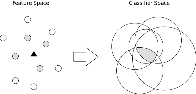
Figure 1: Selection of KNORA-E. On the left side, $\blacktriangle$ is the test sample, and the darkened samples are the region of competence of the test sample. On the right side, the selected classifiers are darkened. (From [12]).

III Problem Statement

When no classifier correctly classifies all samples in the region of competence of a test sample, KNORA-E reduces the region of competence by removing the sample that is the furthest from $x_{query}$, regardless of its class. Because of that, KNORA-E can change a region of competence that is composed of samples from different classes into a region of competence composed of samples from a single class.

Figure 2 presents the iterations of KNORA-E ($K=5$) for the classification of a test sample ($x_{query}$) when no classifier correctly classifies all samples in the region of competence ($\Psi$) of $x_{query}$. In this figure, $\blacktriangle$ is the test sample, the dotted line delimits the region of competence, $A$, $B$, $C$, $D$, and $E$ are the $K$ nearest neighbors of $x_{query}$ in the validation set, $c1$ and $c2$ are classifiers and the continuous straight lines are their decision boundaries. The markers ${\color[rgb]{0,0,1}\scalerel*{\addvbuffer[-.15pt-.6pt]{$\circ$}}{\blacksquare}}$ and ${\color[rgb]{1,0,0}\blacksquare}$ represent samples from different classes, and the test sample is from the class "${\color[rgb]{0,0,1}\scalerel*{\addvbuffer[-.15pt-.6pt]{$\circ$}}{\blacksquare}}$".

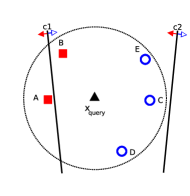
(a) 1st iteration of KNORA-E.

(b) 2nd iteration of KNORA-E.

(c) 3rd iteration of KNORA-E.

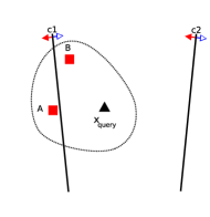
(d) 4th iteration of KNORA-E.

Figure 2: KNORA-E iterations when no classifier correctly classifies all samples in the region of competence of the test sample. The $\blacktriangle$ is the test sample, the markers ${\color[rgb]{0,0,1}\circ}$ and ${\color[rgb]{1,0,0}\blacksquare}$ are samples from different classes in the region of competence of the test sample, and the class of the test sample is "${\color[rgb]{0,0,1}\circ}$". (Adapted from [15]).

In the scenario from Figure 2, in the first and second iterations (Figure 2a and 2b) no classifier correctly classifies all samples in $\Psi$, so KNORA-E removes the samples $E$ and $D$ from $\Psi$, in the first and second iterations, respectively.

In the third iteration (Figure 2c), again, no classifier correctly classifies all samples in $\Psi$, so KNORA-E removes the sample that is the furthest from $x_{query}$, $C$, (the last remaining sample of class "${\color[rgb]{0,0,1}\scalerel*{\addvbuffer[-.15pt-.6pt]{$\circ$}}{\blacksquare}}$" in $\Psi$), leaving only two samples of the class "${\color[rgb]{1,0,0}\blacksquare}$" in $\Psi$. In the fourth iteration (Figure 2d), the classifier $c2$ correctly classifies all samples in $\Psi$ ($A$ and $B$), so KNORA-E selects $c2$, misclassifying the test sample.

This is an issue because when the region of competence of the test sample has samples from different classes, KNORA-E may change the region of competence in such a way that it is no longer a good representation of the local region of the test sample. This behavior is not ideal because classifiers that classify all samples in the region of competence as "${\color[rgb]{1,0,0}\blacksquare}$" (such as $c2$) are selected. This is a problem especially when dealing with imbalanced dataset, where a region of competence with samples from the minority class (class with few samples) can be changed into a region with only samples from the majority class (class with many samples), even though the minority class is usually the class of interest.

IV Proposed Techniques

IV-A KNORA-Borderline

The $K$-Nearest Oracles-Borderline (KNORA-B) is a DES technique based on KNORA-E that maintains the classes represented in the original region of competence of the test sample when reducing the region of competence.

Given a test sample $x_{query}$, KNORA-B finds its region of competence ($\Psi$) by selecting the $K$ nearest neighbors of $x_{query}$ in the validation set $\mathcal{D}_{SEL}$. Then, KNORA-B selects all classifiers that correctly classify all $K$ samples in $\Psi$. If no classifier correctly classifies all samples in $\Psi$, KNORA-B reduces $\Psi$ by removing the sample that is the furthest ($\Psi_{b}$) from $x_{query}$, only if all classes represented in $\Psi$ are still represented in $\Psi/\Psi_{b}$, otherwise, KNORA-B evaluates the removal of the next furthest sample ($\Psi_{b-1}$). The process repeats until at least one classifier is selected. If KNORA-B reaches a state in which it is not possible to remove any sample from $\Psi$ while maintaining the set of classes, KNORA-B uses the KNORA-E rule over the original region of competence.

Algorithm 1 presents the KNORA-B pseudocode. $x_{query}$ is the test sample, $C$ is the pool of classifiers, $\mathcal{D}_{SEL}$ is the validation set, and $K$ is the size of the region of competence. First, KNORA-B initializes EoC as an empty list to insert the selected classifiers (Line 1), it then selects the region of competence $\Psi$ of $x_{query}$ by applying the $K$-nearest neighbors on $\mathcal{D}_{SEL}$ (Line 2), and stores this initial region of competence in $\Psi_{original}$ (Line 3). Next, until at least one classifier is selected or until the region of competence is empty (Line 4), KNORA-B tries to select all classifiers that correctly classify all samples in $\Psi$ (Line 5 - 9), if no classifier is selected KNORA-B reduces the region of competence and the process repeats (Lines 10 - 12). If the region of competence can no longer be reduced, and no classifier was selected, KNORA-B performs the fallback selection (Lines 14 - 16) - the fallback selection of KNORA-B is the KNORA-E procedure. Finally, KNORA-B returns the selected ensemble of classifiers.

Algorithm 1 KNORA-B

0:  $\mathcal{C}$: pool of classifiers

0:  $\mathcal{D}_{SEL}$: validation set

0:  $x_{query}$: test sample

0:  $K$: size of the region of competence

1:  EoC $\leftarrow$ ensemble of classifiers

2:  $\Psi\leftarrow K$ nearest neighbors of $x_{query}$ in $\mathcal{D}_{SEL}$

3:  $\Psi_{original}\leftarrow\Psi$

4:  while Empty(EoC) $\land$ $\neg$Empty($\Psi$) do

5:     for all $c_{i}$ in $\mathcal{C}$ do

6:        if $c_{i}$ correctly classifies all samples in $\Psi$ then

7:           EoC $\leftarrow$ EoC $\cup$ $c_{i}$

8:        end if

9:     end for

10:     if EoC is empty then

11:        $\Psi\leftarrow$reduced_region_of_competence($x_{query},\Psi$)

12:     end if

13:  end while

14:  if EoC is empty then

15:     EoC $\leftarrow$ fallback_selection($C,\Psi_{original},x_{query},K$)

16:  end if

17:  return  EoC

KNORA-B differs from KNORA-E in the reduced region of competence procedure applied when no classifier correctly classifies all samples in the region of competence ($\Psi$). Algorithm 2 presents the region of competence reduction process. Given a test sample $x_{query}$ and the region of competence $\Psi$, KNORA-B gets the size $S$ of the region of competence (Line 1), and assigns that to a variable $b$ (Line 2). Now, until the region of competence is not reduced and $b$ is greater than zero (Line 3), KNORA-B gets the b-th nearest sample (starts with $b=$ SizeOf($\Psi$), that is, from the furthest to the nearest) of $x_{query}$ ($\Psi_{b}$) in $\Psi$ (Line 4), and evaluates if all classes represented in $\Psi$ are still represented if $\Psi_{b}$ is removed from $\Psi$. If so, $\Psi_{b}$ is removed from $\Psi$, otherwise, $b$ is decreased (Lines 5 - 9). If no sample was removed from $\Psi$, this means that no reduction was possible (there is only one sample from each class that was represented in the original region of competence), then $\Psi$ is assigned to an empty set (Lines 11 - 13) so that KNORA-B can use the fallback. Finally, the reduced region of competence is returned (Line 14).

Algorithm 2 KNORA-B - Reduced Region of Competence

0:  $x_{query}$: test sample

0:  $\Psi$: region of competence of $x_{query}$

1:  $S\leftarrow$ SizeOf($\Psi$)

2:  $b\leftarrow$ S

3:  while SizeOf($\Psi$) $=S$ and $b>0$ do

4:     $\Psi_{b}\leftarrow$ b-th nearest from $x_{query}$ in $\Psi$

5:     if Set(classes($\Psi/\Psi_{b}$)) $=$ Set(classes($\Psi$)) then

6:        $\Psi\leftarrow\Psi/\Psi_{b}$

7:     else

8:        $b\leftarrow b-1$

9:     end if

10:  end while

11:  if $\textit{SizeOf($\Psi$)}=S$ then

12:     $\Psi\leftarrow\emptyset$

13:  end if

14:  return  $\Psi$

(a) 1st iteration of KNORA-B.

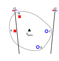
(b) 2nd iteration of KNORA-B.

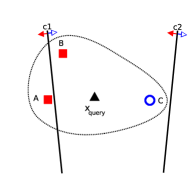
(c) 3rd iteration of KNORA-B.

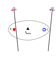
(d) 4th iteration of KNORA-B.

Figure 3: KNORA-B iterations when no classifier correctly classifies all samples in the region of competence of the test sample. The $\blacktriangle$ is the test sample, the markers ${\color[rgb]{0,0,1}\circ}$ and ${\color[rgb]{1,0,0}\blacksquare}$ are samples from different classes in the region of competence of the test sample, and the class of the test sample is "${\color[rgb]{0,0,1}\circ}$". (Adapted from [15]).

Figure 3 presents the iterations of KNORA-B ($K=5$) for the classification of a test sample ($x_{query}$) when no classifiers correctly classify all samples in the region of competence ($\Psi$) of $x_{query}$. In this figure, $\blacktriangle$ is the test sample, the dotted line delimits the region of competence, $A$, $B$, $C$, $D$, and $E$ are the $K$ nearest neighbors of $x_{query}$ in the validation set, $c1$ and $c2$ are classifiers and the continuous straight lines are their decision boundaries. The markers ${\color[rgb]{0,0,1}\scalerel*{\addvbuffer[-.15pt-.6pt]{$\circ$}}{\blacksquare}}$ and ${\color[rgb]{1,0,0}\blacksquare}$ are samples from different classes, and the test sample is from the class "${\color[rgb]{0,0,1}\scalerel*{\addvbuffer[-.15pt-.6pt]{$\circ$}}{\blacksquare}}$".

In the scenario from Figure 3, in the first and second iterations (Figure 3a and 3b) no classifier correctly classifies all samples in $\Psi$, so, KNORA-B removes the sample that is the furthest from $x_{query}$, respectively, $E$ and $D$, from $\Psi$. In the third iteration (Figure 3c), again, no classifier correctly classifies all samples in $\Psi$, but instead of removing the furthest sample $C$, leaving only samples from the class "${\color[rgb]{1,0,0}\blacksquare}$" in $\Psi$, KNORA-B removes the second furthest sample $B$, maintaining samples from both classes "${\color[rgb]{0,0,1}\scalerel*{\addvbuffer[-.15pt-.6pt]{$\circ$}}{\blacksquare}}$" and "${\color[rgb]{1,0,0}\blacksquare}$" in $\Psi$. In the fourth iteration (Figure 3d), the classifier $c1$ correctly classifies all samples in $\Psi$ ($A$ and $C$), so, KNORA-B selects $c1$ and correctly classifies the test sample as being from the class "${\color[rgb]{0,0,1}\scalerel*{\addvbuffer[-.15pt-.6pt]{$\circ$}}{\blacksquare}}$".

Comparing Figure 2 with Figure 3, we can see that KNORA-B is better in selecting classifiers for the classification of the test sample that has a region of competence with samples of different classes. While KNORA-E selects $c2$, a base classifier that classifies all samples in $\Psi$ as being from the same class "${\color[rgb]{1,0,0}\blacksquare}$", and misclassifies the test sample, KNORA-B selects $c1$, a base classifier that correctly classifies samples from different classes in $\Psi$, correctly classifying the test sample.

IV-B KNORA-Borderline-Imbalanced

When dealing with specific problems such as imbalanced datasets, KNORA-B can remove a minority class sample that is closer to the test sample instead of a majority class sample that is the furthest. This behavior is not desired in the context of imbalanced datasets, in which the minority class (class with few samples) is the class of interest [16].

KNORA-Borderline-Imbalanced (KNORA-BI) is a variation of KNORA-B that has a different reduced region of competence reduction procedure that allows the reduction of a region of competence that is composed of samples from the majority and minority classes into a region of competence composed only of samples from the minority class. By doing so, KNORA-BI favors only the minority class when reducing the region of competence.

KNORA-BI region of competence reduction pseudocode is presented in Algorithm 3. Given a test sample $x_{query}$ the region of competence $\Psi$, and the minority class class_min, KNORA-BI gets the size $S$ of the region of competence (Line 1) and assigns that to a variable $b$ (Line 2). Now, until the region of competence is not reduced and $b$ is greater than zero (Line 3), KNORA-BI gets the b-th nearest sample (starts with $b=$ SizeOf($\Psi$), that is, from the furthest to the nearest) of $x_{query}$ ($\Psi_{b}$) in $\Psi$ (Line 4), if $\Psi_{b}$ is not from the minority class or if all classes represented in $\Psi$ are still represented when $\Psi_{b}$ is removed from $\Psi$, then, $\Psi_{b}$ is removed from $\Psi$, otherwise, $b$ is decreased (Lines 5 - 9). If no sample is removed from $\Psi$ and $b$ reaches zero, $\Psi$ is assigned to an empty set (Lines 11 - 13). Thus, KNORA-BI can use the fallback. Finally, the reduced region of competence is returned (Line 14).

Algorithm 3 KNORA-BI - Reduced Region of Competence

0:  $x_{query}$: test sample

0:  $\Psi$: region of competence of $x_{query}$

0:  class_min: minority class

1:  $S\leftarrow$ SizeOf($\Psi$)

2:  $b\leftarrow$ S

3:  while SizeOf($\Psi$) $=S$ and $b>0$ do

4:     $\Psi_{b}\leftarrow$ b-th nearest from $x_{query}$ in $\Psi$

5:     if Class($\Psi_{b}$) $\neq$ class${}_{min}\lor$ Set(classes($\Psi/\Psi_{b}$)) $=$ Set(classes($\Psi$)) then

6:        $\Psi\leftarrow\Psi/\Psi_{b}$

7:     else

8:        $b\leftarrow b-1$

9:     end if

10:  end while

11:  if $\textit{SizeOf($\Psi$)}=S$ then

12:     $\Psi\leftarrow\emptyset$

13:  end if

14:  return  $\Psi$

Considering the examples from Figure 2 and 3, KNORA-BI region of competence reduction procedure reduces the region of competence in such a way that:

• if the class "${\color[rgb]{0,0,1}\scalerel*{\addvbuffer[-.15pt-.6pt]{$\circ$}}{\blacksquare}}$" is the majority class, KNORA-BI acts as exemplified in Figure 2 - as it allows the removal of all majority class samples, leaving all minority class samples.

• if the class "${\color[rgb]{0,0,1}\scalerel*{\addvbuffer[-.15pt-.6pt]{$\circ$}}{\blacksquare}}$" is the minority class, KNORA-BI acts as exemplified in Figure 3 - as it does not allow the removal of all minority class samples.

V Experiments

We evaluated KNORA-B and KNORA-BI using 40 datasets as proposed in [15]. The datasets were taken from the imbalanced datasets module in the Knowledge Experiments based on Evolutionary Learning (KEEL) repository [18]. Table I presents the details about the datasets used in our experiments: label, name, number of features, number of samples, and imbalance ratio (IR).

TABLE I: Summary of the 40 datasets used in the experiments: label, name, number of features, number of samples, and imbalance ratio (from [15]).

Label	Name	#Feats.	#Samples	IR
1	glass1	9	214	1.82
2	ecoli0vs1	7	220	1.86
3	wisconsin	9	683	1.86
4	pima	8	768	1.87
5	iris0	4	150	2.00
6	glass0	9	214	2.06
7	yeast1	8	1484	2.46
8	vehicle2	18	846	2.88
9	vehicle1	18	846	2.9
10	vehicle3	18	846	2.99
11	glass0123vs456	9	214	3.2
12	vehicle0	18	846	3.25
13	ecoli1	7	336	3.36
14	new-thyroid1	5	215	5.14
15	new-thyroid2	5	215	5.14
16	ecoli2	7	336	5.46
17	segment0	19	2308	6.00
18	glass6	9	214	6.38
19	yeast3	8	1484	8.10
20	ecoli3	7	336	8.60
21	yeast-2vs4	8	514	9.08
22	yeast-05679vs4	8	528	9.35
23	vowel0	13	988	9.98
24	glass-016vs2	9	192	10.29
25	glass2	9	214	11.59
26	shuttle-c0vsc4	9	1829	13.87
27	yeast-1vs7	7	459	14.30
28	glass4	9	214	15.47
29	ecoli4	7	336	15.80
30	page-blocks-13vs4	10	472	15.86
31	glass-0-1-6_vs_5	9	184	19.44
32	shuttle-c2-vs-c4	9	129	20.50
33	yeast-1458vs7	8	693	22.10
34	glass5	9	214	22.78
35	yeast-2vs8	8	482	23.10
36	yeast4	8	1484	28.10
37	yeast-1289vs7	8	947	30.57
38	yeast5	8	1484	32.73
39	ecoli-0137vs26	7	281	39.14
40	yeast6	8	1484	41.40

For each dataset, the data was partitioned using the stratified 5-fold cross-validation (1 fold used for testing, and 4 folds for validation/training) followed by a stratified 4-fold cross-validation (the 4 folds into validation/training divided in 1 for validation and 3 for training), resulting in 20 replications for each dataset using 20% for testing, 20% for validation, and 60% for training.

The analysis is conducted using 8 DES techniques from the literature, their respective FIRE-DES versions (using the F prefix), and 3 state-of-the-art DES techniques. Table II shows the dynamic selection techniques used in our experiments, their categories and references. Following the approach using in [15], we use a pool of classifiers composed of 100 Perceptrons generated using the Bootstrap AGGregatING (Bagging) technique [19], and a region of competence size $K=7$.

TABLE II: Dynamic selection techniques considered in the experiments (From [15]).

Technique	Category	Reference
DES
Overall Local Accuracy (OLA)	Accuracy	Woods et al. [20]
Local Class Accuracy (LCA)	Accuracy	Woods et al. [20]
A Priori (APri)	Probabilistic	Giacinto et al. [21]
A Posteriori (APos)	Probabilistic	Giacinto et al. [21]
Multiple Classifier Behavior (MCB)	Behavior	Giacinto et al. [22]
Dynamic Selection KNN (DSKNN)	Diversity	Santana et al. [23]
K-Nearests Oracles Union (KNORA-U)	Oracle	Ko et al. [12]
K-Nearests Oracles Eliminate (KNORA-E)	Oracle	Ko et al. [12]
State-of-the-art
Randomized Reference Classifier (RRC)	Probabilistic	Woloszynski et al. [24]
META-DES	Meta-learning	Cruz et al. [25]
META-DES.Oracle	Meta-learning	Cruz et al. [26]

Following the approach in [15], we used the Area Under the ROC Curve (AUC) [27] for performance evaluation since it is a suitable metric for binary imbalanced datasets [16] [15]. We also used the Wilcoxon Signed Rank Test [28] [29] and the Sign Test [30] to perform a pairwise comparison of the proposed techniques with the techniques from the literature.

V-A Results

Table III presents the overall results. For each technique, the table shows: the mean AUC and standard deviation, the average ranking, and the p-value and result of the Wilcoxon Signed Rank Test comparing KNORA-B and KNORA-BI with the DES technique ($+$/$=$/$-$ signs mean the proposed technique had statistically better, equal, and worse classification performance considering a confidence level $\alpha=0.05$).

TABLE III: Overall results.

DES	AUC	RANK	KNORA-B (p-value)		KNORA-BI (p-value)
KNORA-BI	0.8136 (0.0743)	6.80	0.9999	$-$	$N/A$
META.O	0.8067 (0.0649)	8.16	0.9509	$-$	0.3454	$=$
META	0.8100 (0.0635)	8.20	0.9742	$-$	0.4362	$=$
FKNORA-U	0.8081 (0.0765)	8.38	0.9712	$-$	0.1009	$=$
FMCB	0.8058 (0.0760)	8.80	0.9235	$=$	0.0921	$=$
FKNORA-BI	0.8083 (0.0758)	9.01	0.9976	$-$	0.0003	$+$
FKNORA-E	0.8055 (0.0768)	9.59	0.9962	$-$	0.0002	$+$
FKNORA-B	0.8042 (0.0772)	10.34	0.9860	$-$	0.0001	$+$
KNORA-E	0.8003 (0.0703)	10.66	0.8298	$=$	0.0002	$+$
KNORA-B	0.7989 (0.0721)	11.28	$N/A$		$5.60\times e^{-6}$	$+$
FDSKNN	0.8006 (0.0767)	11.43	0.5250	$=$	$2.00\times e^{-6}$	$+$
FLCA	0.7946 (0.0777)	11.84	0.5554	$=$	$8.30\times e^{-6}$	$+$
RRC	0.7934 (0.0658)	12.26	0.1805	$=$	0.0057	$+$
FOLA	0.8017 (0.0767)	12.97	0.5026	$=$	$3.80\times e^{-6}$	$+$
FAPRI	0.7930 (0.0802)	13.10	0.1940	$=$	$1.60\times e^{-6}$	$+$
LCA	0.7809 (0.0737)	13.30	0.0332	$+$	$7.20\times e^{-6}$	$+$
DSKNN	0.7728 (0.0602)	13.32	0.0107	$+$	$6.10\times e^{-5}$	$+$
OLA	0.7911 (0.0709)	13.60	0.0623	$=$	$1.40\times e^{-7}$	$+$
KNORA-U	0.7560 (0.0548)	15.39	0.0002	$+$	$6.80\times e^{-6}$	$+$
FAPOS	0.7681 (0.0809)	15.86	0.0001	$+$	$1.40\times e^{-7}$	$+$
APRI	0.7537 (0.0628)	16.38	$3.20\times e^{-5}$	$+$	$9.80\times e^{-7}$	$+$
APOS	0.7380 (0.0658)	18.01	$1.10\times e^{-5}$	$+$	$4.70\times e^{-7}$	$+$
MCB	0.7443 (0.0566)	17.32	$2.10\times e^{-6}$	$+$	$6.40\times e^{-7}$	$+$

Table III show that KNORA-BI achieved the highest mean AUC ($0.8136$) and the best average ranking ($6.80$), outperforming all techniques considered in this work. Moreover, it statistically outperformed 18 out of 22 techniques according to the Wilcoxon Signed Rank test. Table III also shows that KNORA-B was not as good as KNORA-BI, achieving the 12th best AUC ($0.7989$), and being statistically equivalent to KNORA-E ($0.8003$). However, it was only statistically outperformed by 7 out of 22 techniques, where 3 of those are variations of the techniques proposed in this paper (KNORA-BI, FKNORA-B, and FKNORA-BI).

In addition, FKNORA-B ($0.8042$) outperformed KNORA-B ($0.7989$) with statistical confidence, meaning FIRE-DES caused a significant increase in classification performance in KNORA-B. This increase in AUC is explained in the scenario that no classifier was selected and the region of competence has only one sample from each class remaining. In this scenario, KNORA-B applies KNORA-E on the entire pool of classifiers while FKNORA-B applies KNORA-E on the set of pre-selected classifiers (avoiding the selection of incompetent classifiers that classify all samples in the region of competence as being from the same class).

On the other hand, KNORA-BI ($0.8136$) outperformed FKNORA-BI ($0.8083$) with statistical confidence, meaning FIRE-DES caused a significant decrease in classification performance in KNORA-BI. KNORA-BI allows the region of competence to be reduced until there is only minority class samples, allowing to the selection of classifiers that classify all samples in the region of competence as minority class samples, while FKNORA-BI does not allow the selection of such classifiers. Because the minority class is so rare, preventing a DES technique from selecting a classifier that classifies all samples in the region of competence as minority class sample is not advantageous, specially because correctly classifying 1 minority class sample has a higher impact than misclassifying 1 majority class sample, which explains why KNORA-BI was better without FIRE-DES.

Figure 4 presents a pairwise comparison using the Sign Test [30], calculated using the wins, ties, and losses achieved by the KNORA-B compared to other techniques (Figure 4a) and by the KNORA-BI compared to other techniques (Figure 4b).

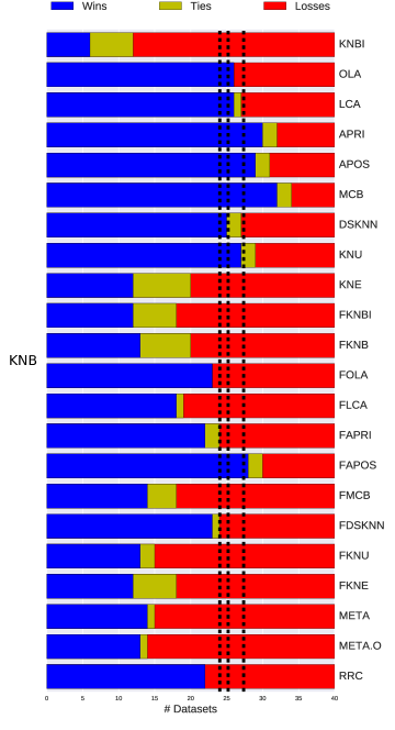
(a) Comparison of KNORA-B and other techniques.

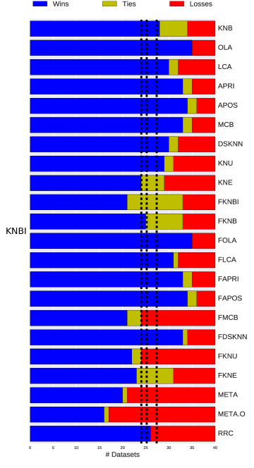
(b) Comparison of KNORA-BI and other techniques.

Figure 4: Classification performance comparison of KNORA-B with different DES techniques (Figure 4a) and KNORA-BI with different DES techniques (Figure 4b) in terms of wins, ties and losses considering the average AUC in the 40 datasets. The dashed lines (left to right) illustrates the critical values $n_{c}=\{24.05,25.20,27.37\}$ considering significance levels of $\alpha=\{0.10,0.05,0.01\}$, respectively.

For a comparison between one of the proposed techniques and a technique T, the null hypothesis $H_{0}$ was that the proposed technique is not statistically different than T, and a rejection of $H_{0}$ meant that the proposed technique is statistically better than T. $H_{0}$ is rejected if the number of wins plus half of the number of ties is greater or equal to $n_{c}$ (Equation 1):

$$n_{c}=\dfrac{n_{exp}}{2}+z_{\alpha}\times\dfrac{\sqrt[2]{n_{exp}}}{2}$$ (1)

where $n_{exp}=40$ (the number of experiments), $n_{c}=\{24.05,25.20,27.37\}$, respectively for the levels of significance $\alpha=\{0.10,0.05,0.01\}$.

Figure 4a shows that, considering $\alpha=0.05$, KNORA-B statistically outperformed 7 out of the 8 regular DES techniques, being only statistically equivalent to KNORA-E. Comparing with FIRE-DES framework, KNORA-B outperformed only FAPOS (the worst of FIRE-DES in our experiments). KNORA-B was not better than any of the state-of-art DES techniques.

On the other hand, Figure 4b shows that overall KNORA-BI statistically outperformed a significant number of techniques studied (18 out of 22), considering a significance level $\alpha=0.05$. The only exceptions being the FMCB, FKNORA-U, META-DES, and META-DES.Oracle.

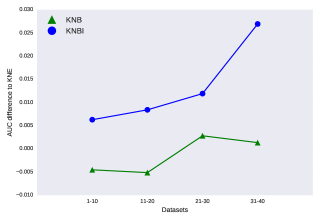
Figure 5: AUC difference between KNORA-B and KNORA-E, and between KNORA-BI and KNORA-E.

Figure 5 presents the average AUC difference from KNORA-B and KNORA-BI to KNORA-E considering the datasets 1-10, 11-20, 21-30, and 31-40. This figure shows that KNORA-B is better than KNORA-E optimally in 21-30 and slightly better in 31-40, while KNORA-BI was always better than KNORA-E (the more the imbalance ratio the higher the difference). This confirms that for all imbalance levels KNORA-BI was better than KNORA-E, while KNORA-B was only better than KNORA-B for high imbalance level.

Based on the results, we can state with confidence that KNORA-B achieved statistically equivalent performance of KNORA-E, and KNORA-BI statistically outperformed KNORA-E and all other techniques considered in this experiment.

VI Conclusion

In this paper, we proposed two DES techniques: K-Nearest Oracles Borderline (KNORA-B) and K-Nearest Oracles Borderline Imbalanced (KNORA-BI). KNORA-B is a DES technique based on KNORA-E that selects all classifiers that correctly classify all samples in the region of competence. If no classifier is selected, KNORA-B reduces the region of competence maintaining the at least one sample from each class in the original region of competence. KNORA-BI is a variation of KNORA-B that reduces the region of competence, but maintaining at least one sample of the minority class (if such sample exists in the original region of competence).

We conducted experiments using 40 datasets from the KEEL software [18] with different levels of imbalance, and compared KNORA-B and KNORA-BI with 8 regular DES techniques, 8 FIRE-DES techniques, and 3 state-of-the-art DES techniques.

Results showed that KNORA-B had statistically equivalent performance of KNORA-E, and KNORA-BI statistically outperformed KNORA-E in classification performance. In fact, KNORA-BI achieved the best average classification performance over all DES techniques considered in our experiments, including the state-of-the-art DES techniques.

References

- [1] M. Woźniak, M. Graña, and E. Corchado, “A survey of multiple classifier systems as hybrid systems,” Information Fusion, vol. 16, pp. 3–17, 2014.
- [2] L. I. Kuncheva, Combining pattern classifiers: methods and algorithms. John Wiley & Sons, 2004.
- [3] S. Singh and M. Singh, “A dynamic classifier selection and combination approach to image region labelling,” Signal Processing: Image Communication, vol. 20, no. 3, pp. 219–231, 2005.
- [4] R. M. Cruz, G. D. Cavalcanti, R. Tsang, and R. Sabourin, “Feature representation selection based on classifier projection space and oracle analysis,” Expert Systems with Applications, vol. 40, no. 9, pp. 3813–3827, 2013.
- [5] L. Batista, E. Granger, and R. Sabourin, “Improving performance of hmm-based off-line signature verification systems through a multi-hypothesis approach,” International Journal on Document Analysis and Recognition, vol. 13, no. 1, pp. 33–47, 2010.
- [6] M. Jahrer, A. Töscher, and R. Legenstein, “Combining predictions for accurate recommender systems,” in International Conference on Knowledge Discovery and Data Mining. ACM, 2010, pp. 693–702.
- [7] S. Bhattacharyya, S. Jha, K. Tharakunnel, and J. C. Westland, “Data mining for credit card fraud: A comparative study,” Decision Support Systems, vol. 50, no. 3, pp. 602–613, 2011.
- [8] M. De-la Torre, E. Granger, R. Sabourin, and D. O. Gorodnichy, “An adaptive ensemble-based system for face recognition in person re-identification,” Machine Vision and Applications, vol. 26, no. 6, pp. 741–773, 2015.
- [9] A. Puurula, J. Read, and A. Bifet, “Kaggle lshtc4 winning solution,” arXiv preprint arXiv:1405.0546, 2014.
- [10] Y. Koren, “The bellkor solution to the netflix grand prize,” Netflix prize documentation, vol. 81, 2009.
- [11] R. M. Bell and Y. Koren, “Lessons from the netflix prize challenge,” ACM SIGKDD Explorations Newsletter, vol. 9, no. 2, pp. 75–79, 2007.
- [12] A. H. Ko, R. Sabourin, and A. S. Britto Jr, “From dynamic classifier selection to dynamic ensemble selection,” Pattern Recognition, vol. 41, no. 5, pp. 1718–1731, 2008.
- [13] R. M. Cruz, R. Sabourin, and G. D. Cavalcanti, “Dynamic classifier selection: Recent advances and perspectives,” Information Fusion, vol. 41, pp. 195–216, 2018.
- [14] A. S. Britto, R. Sabourin, and L. E. Oliveira, “Dynamic selection of classifiers—a comprehensive review,” Pattern Recognition, vol. 47, no. 11, pp. 3665–3680, 2014.
- [15] D. V. Oliveira, G. D. Cavalcanti, and R. Sabourin, “Online pruning of base classifiers for dynamic ensemble selection,” Pattern Recognition, vol. 72, pp. 44–58, 2017.
- [16] V. López, A. Fernández, S. García, V. Palade, and F. Herrera, “An insight into classification with imbalanced data: Empirical results and current trends on using data intrinsic characteristics,” Information Sciences, vol. 250, pp. 113–141, 2013.
- [17] L. I. Kuncheva, “A theoretical study on six classifier fusion strategies,” IEEE Transactions on pattern analysis and machine intelligence, vol. 24, no. 2, pp. 281–286, 2002.
- [18] J. Alcalá, A. Fernández, J. Luengo, J. Derrac, S. García, L. Sánchez, and F. Herrera, “KEEL data-mining software tool: Data set repository, integration of algorithms and experimental analysis framework,” Journal of Multiple-Valued Logic and Soft Computing, vol. 17, no. 2-3, pp. 255–287, 2010.
- [19] L. Breiman, “Bagging predictors,” Machine learning, vol. 24, no. 2, pp. 123–140, 1996.
- [20] K. Woods, W. P. Kegelmeyer, and K. W. Bowyer, “Combination of multiple classifiers using local accuracy estimates,” IEEE Transactions on Pattern Analysis and Machine Intelligence, vol. 19, no. 4, pp. 405–410, 1997.
- [21] G. Giacinto and F. Roli, “Methods for dynamic classifier selection,” in International Conference on Image Analysis and Processing. IEEE, 1999, pp. 659–664.
- [22] ——, “Dynamic classifier selection based on multiple classifier behaviour,” Pattern Recognition, vol. 34, no. 9, pp. 1879–1881, 2001.
- [23] A. Santana, R. G. Soares, A. M. Canuto, and M. C. de Souto, “A dynamic classifier selection method to build ensembles using accuracy and diversity,” in Brazilian Symposium on Neural Networks. IEEE, 2006, pp. 36–41.
- [24] T. Woloszynski and M. Kurzynski, “A probabilistic model of classifier competence for dynamic ensemble selection,” Pattern Recognition, vol. 44, no. 10, pp. 2656–2668, 2011.
- [25] R. M. Cruz, R. Sabourin, G. D. Cavalcanti, and T. I. Ren, “META-DES: A dynamic ensemble selection framework using meta-learning,” Pattern Recognition, vol. 48, no. 5, pp. 1925–1935, 2015.
- [26] R. M. Cruz, R. Sabourin, and G. D. Cavalcanti, “META-DES.Oracle: Meta-learning and feature selection for dynamic ensemble selection,” Information Fusion, vol. 38, pp. 84–103, 2017.
- [27] A. P. Bradley, “The use of the area under the ROC curve in the evaluation of machine learning algorithms,” Pattern Recognition, vol. 30, no. 7, pp. 1145–1159, 1997.
- [28] A. Benavoli, G. Corani, and F. Mangili, “Should we really use post-hoc tests based on mean-ranks,” Journal of Machine Learning Research, vol. 17, no. 5, pp. 1–10, 2016.
- [29] F. Wilcoxon, “Individual comparisons by ranking methods,” Biometrics bulletin, vol. 1, no. 6, pp. 80–83, 1945.
- [30] J. Demšar, “Statistical comparisons of classifiers over multiple data sets,” Journal of Machine Learning Research, vol. 7, no. 1, pp. 1–30, 2006.