Errors, chaos and the collisionless limit

Abstract

We simultaneously study the dynamics of the growth of errors and the question of the faithfulness of simulations of $N$-body systems. The errors are quantified through the numerical reversibility of small-$N$ spherical systems, and by comparing fixed-timestep runs with different stepsizes. The errors add randomly, before exponential divergence sets in, with exponentiation rate virtually independent of $N$, but scale saturating as $\sim 1/\sqrt{N}$, in line with theoretical estimates presented. In a third phase, the growth rate is initially driven by multiplicative enhancement of errors, as in the exponential stage. It is then qualitatively different for the phase space variables and mean field conserved quantities (energy and momentum); for the former, the errors grow systematically through phase mixing, for the latter they grow diffusively. For energy, the $N$-variation of the ‘relaxation time’ of error growth follows the $N$-scaling of two-body relaxation. This is also true for angular momentum in the fixed stepsize runs, although the associated error threshold is higher and the relaxation time smaller. Due to shrinking saturation scales, the information loss associated with the exponential instability decreases with $N$ and the dynamical entropy vanishes at any finite resolution as $N\rightarrow\infty$. A distribution function depending on the integrals of motion in the smooth potential is decreasingly affected. In this sense there is convergence to the collisionless limit, despite the persistence of exponential instability on infinitesimal scales. Nevertheless, the slow $N$-variation in its saturation points to the slowness of the convergence.

1 Introduction

The dynamics of the growth of small perturbations to the trajectories of Newtonian $N$-body gravitational systems is of importance, both from a theoretical point of view and in terms of its implications on the accuracy and faithfulness of numerical simulations. Theoretically, $N$-body systems are expected to tend to the collisionless limit as $N$ increases, yet this can be rigorously proven only when the two body potential is smooth (Braun & Hepp 1977), which is the case in softened systems but not for point particle interactions. For unsoftened systems, which is the case of actual stellar systems for example, a peculiar phenomenon concerns the persistence of the exponential divergence between nearby trajectories. This takes place at rate that does not decrease with $N$, even for configurations with corresponding smooth potentials that support only regular orbits (Miller 1964; Kandrup & Smith 1991; Goodman, Heggie & Hut 1993, hereafter GHH; Hemsendorf & Merritt 2002). It thus appears to be in direct contradiction with the predictions of the collisionless limit; in this limit, the orbits are characteristic curves of the collisionless Boltzmann equation and, being regular, should not display exponential instability, which is characteristic of chaotic systems.

Numerically identified dynamical chaos normally comes with important physical consequences (e.g., Lichtenberg & Lieberman 1992; Contopoulos 2002). In principle, therefore, it is not a priori obvious that the apparently ’chaotic’ nature of the $N$-body problem does not lead to any physically relevant phenomena. On the other hand, the effects associated with the divergence of trajectories can appear as artifacts that affect particle simulations, where particle numbers are usually much smaller than in the physical systems modelled, and various approximations, effectively perturbing the dynamical system in a complicated manner, are made. Thus, the collisionless limit may not be reproduced in simulations because the dynamics do not converge to it, even in principle, or because the numerical image does not.

$N$-body simulations have long been indispensable to understanding structure formation in the universe, and the evolution of galaxies, galaxy clusters and stellar clusters (e.g. Heggie & Hut 2003; Dehnen & Read 2011; Springel 2016). Yet, despite decades of steady increase in sophistication, relatively little progress has been made in assessing their accuracy, or even the qualitative faithfulness of the results obtained to the ‘true’ dynamics. Indeed, more efficient force calculation schemes normally entail larger errors than direct force evaluations (see however Dehnen 2014 for a counter-example). In addition, an estimate of the local or global error in the integration of the equations of motion is not in general available.

The exponential instability places a fundamental limitations on the accuracy of simulations by inflating any errors arising from approximate force evaluations, as well roundoff errors arising from finite arithmetic and truncation errors associated with finite integration timesteps. In the absence of any intrinsic divergence in the solutions, the errors scale linearly, or slower, with the number of timesteps (e.g., Press et. al. 2007). This will also be the case with the action and angle variables of systems supporting regular trajectories (for a general discussion of regular versus chaotic motion in the context of stellar dynamics see, e.g., Binney & Tremaine 2008; hereafter BT). As we discuss in Section 3.1, this implies that accurate solutions can be obtained by increasing the order of the integrator and decreasing the time-step. A remedy that does not apply in the presence of the exponential instability.

Despite this, it is widely believed that $N$-body simulations do reproduce the correct qualitative behaviour of the modelled systems. In some sense, this is a statistical statement. It embodies the belief that even when the correct trajectories cannot be captured, statistical faithfulness may be retained in terms of the proper rendering of the gross structure of the system, as characterized by the distribution function and the moments derived from it. In this context, confidence in the faithfulness of the simulations stems from the general stability of gross characteristics (e.g., density and mean velocities and velocity dispersions), when large-$N$ systems are simulated from different initial conditions taken from the same statistical distributions. This stability persists even when different simulation techniques are used, though there is no guarantee that all results are not equally wrong. More rigorous justification of the faithfulness of results may be sought in terms of the existence of shadowing trajectories. These are exact solutions that start from nearby initial conditions and remain close to the numerical solutions for the timescales of interest. Their presence, however, is generally quite difficult to prove and has only been studied in idealized cases (Quinlan & Tremaine 1992; Hayes 2003). On the other hand, it is known that at least in models where collective instabilities are present, numerical implementation and associated exponentially inflated error can play an important role in determining the macroscopic evolution (Sellwood & Debattista 2009; Benhaiem et al. 2018). Understanding this role may also be of importance in the context of interpreting the results of cosmological simulations (Thiébaut et. al. 2008; Keller et. al. 2018; Genel et. al. 2018).

The robustness of the results of simulations can also be viewed in terms of the orbital structure, which links intrinsic dynamical properties, related to the stability of trajectories, to questions regarding the accuracy of numerical representation. In general, the phase space of Hamiltonian systems can exhibit a variety of regular and chaotic orbital families (e.g., Lichtenberg & Lieberman 1992; BT), and a numerical method can be said to faithfully represent the dynamics if it qualitatively captures these structures. A $N$-body trajectory formally moves in a $6N$ dimensional phase space; and is, most generally, only constrained by globally conserved quantities, such as the total energy and angular momentum. Nevertheless, in the collisionless limit, as $N\rightarrow\infty$, the $N$-body problem should effectively reduce to that of $N$ independent systems, as each particle moves in the (self consistent) mean field produced by all particles. The relevant phase space structure is six dimensional. If, furthermore, this mean field is time independent and possesses sufficient symmetry, the system is ‘separable’ and the problem is further reduced to that of $3N$ independent one dimensional oscillations or rotations. In a six dimensional phase space, particle trajectories are then confined on tori that can be characterised by conserved quantities, and parametrised for example by action variables, reflecting the amplitudes of the oscillations, and angles following the phases. The difference between phases of orbits parametrised by different values of the actions diverge only linearly in time (BT). This situation, though restricted, forms the basis of much of classical galactic dynamics. It also relates the two aspects of our study: such a configuration can be said to approach the collisionless limit if its dynamics can be parametrised in terms of quantities conserved along trajectories in the smoothed (mean field) potential, and a numerical simulation of such a system is ’faithful’ if it captures this structure. A particularly simple and important example is that of a large-$N$ spherical system in a steady state, where each trajectory should conserve energy and angular momentum. These mean field conserved quantities are the integrals of motion of the smooth potential. This is the case primarily considered here.

A key feature suggesting that the effects of the exponential instability do decrease in importance with increasing $N$, despite the non-saturating rate, comes from theoretical arguments and idealised numerical experiments suggesting that its spatial scale tends to saturate as the particle number increases, even if its rate does not (GHH; Valluri & Merritt 2000; Kandrup & Sideris 2001; Sideris & Kandrup 2002). Indeed, trajectories moving in a ‘gravitational Lorentz gas’ of fixed particles appear to increasingly follow their smooth-potential counterparts as the number of fixed particles is increased. The exponential instability timescale itself also increases with $N$ when softening is introduced (GHH; Huang, Dubinski & Carlberg 1993; El-Zant 2002).

Thus, although divergence between nearby trajectories implies loss of detailed information regarding these, as we will see here, this loss decreases with $N$ as the instability saturates on progressively smaller scales. Furthermore, we find that errors in mean field conserved quantities eventually follow a slow diffusive growth (on a timescale comparable to the two body relaxation time in case of particle energies). This is the case even if the initial exponential divergence affects these quantities in the same way as the phase space variables. Thus, from a dynamical systems point of view, the orbital structure can be well preserved, and the information loss limited, despite the persistence of the local exponential instability on the infinitesimal scale. From a statistical viewpoint, if the integrals of motion are well conserved, the basic features of the collisionless description should hold, as in this limit spherical steady state systems are described by a distribution function depending on those quantities. From a numerical perspective, if the integration preserves the mean field conserved quantities in a way that permits the reproduction of the statistical properties described by the distribution function, the representation is faithful to the collisionless description in this specific sense.

In this context, the purpose of the present study was twofold: to examine the dynamical divergence in both the phase space variables and the mean field conserved quantities of initially nearby trajectories, and to do this in a way that relates the associated information loss to the accuracy and faithfulness of the numerical representation of the dynamics. For this purpose, we examined the time-reversibility of a large number of spherical $N$-body systems integrated with high precision using an adaptive Runge-Kutta method with present error tolerance. In principle, these systems should be exactly time reversible when the velocities are reversed. Nevertheless, this is not generally the case with their numerical image; the exponential divergence of trajectories, and associated loss of information, renders them irreversible if a general integrator is used (e.g. Hoover & Hoover 2012). In the context thus set, a simulation can be considered ‘inaccurate’ on timescales on which information loss leads to irreversibility in the phase space variables, but is only ‘unfaithful’ over timescales on which the mean field conserved quantities in the reversed system differ considerably from the originals. We use this diagnostic in drawing conclusions concerning the implications, physical and numerical, of ‘chaos’ in $N$-body gravitational systems. In addition, in order to better relate to contemporary $N$-body simulations of collisionless systems, we also examine the same aforementioned issues using the widely employed symplectic leapfrog integrator (which has reversible truncation errors when applied to reversible dynamical systems). This is done by comparing the evolution of systems that are started from the same initial conditions but evolved forward in time with different stepsize. We also compare the results using the leapfrog integrator with those obtained using second and fourth order Runge-Kutta methods with fixed stepsize.

In the next section we describe the numerical setup for our simulations and the method through which the estimates of error growth are evaluated. Section 3 constitutes the bulk of this study. We start by delineating the differences, crucial to the interpretation of our results, between systematic, diffusive and exponential evolution of the growth of errors, presenting estimates of the expected numerical errors. We then report the numerical results, which are interpreted by adapting a model due to GHH, which is shown to predict the persistence of systematic growth after the saturation of the exponential divergence. In the case of the phase space variables, this is followed by phase mixing; for the mean field conserved quantities it is followed by the onset of diffusion. We then evaluate ‘relaxation times’, associated with the growth of errors in the different quantities, contrasting the growth of velocity errors with the that in angular momentum and energy. The results of the fixed stepsize runs are presented, before summarising our findings in Section 3.6. In Section 4 we discuss whether $N$-body systems can be characterised as ‘chaotic’ on any non-infinitesimal scale on the phase space as $N\rightarrow\infty$, given the progressively smaller loss of information, particularly as associated with the mean field conserved quantities (a more formal discussion of the relation between chaos, information loss and effective irreversibility is given in the Appendix).

2 Numerical setup

2.1 Reversibility as a probe of numerical accuracy and faithfulness

Newtonian $N$-body systems obey equations where the time variable appears exclusively in second order form. These systems are thus time reversible in principle: for every solution evolved up to a time $t_{f}$, there is a solution — obtained by reversing the velocities at $t_{f}$ and evolving the system for another timespan $t_{f}$ — such that, for $t\geq t_{f}$, ${\bf r}(t)={\bf r}(2t_{f}-t)$ and ${\dot{\bf r}}(t)=-{\dot{\bf r}}(2t_{f}-t)$, where ${\bf r}$ is the $3N$ dimensional coordinate vector of particle positions.

Numerically, however, the situation is generally different. Even assuming that the forces are evaluated to machine precision, there will be roundoff errors in these, as well as in the phase space variables themselves (including the initial conditions). Finite time-stepping also leads to truncation errors. If the errors are sufficiently inflated by intrinsic divergence of trajectories, numerical irreversibility will result, as the accumulating errors in the forward and reversed trajectories diverge. It is of course possible to employ time symmetric algorithms, which are formally reversible when applied to time reversible dynamical systems (Hernandez & Bertschinger 2018; Hairer, Lubich & Wanner 2006, section V.1); the symplectic mapping embodied in the widely used leapfrog integrator is one such scheme. Although the truncation errors are then reversible, floating point errors remain, unless integer or fixed point arithmetic is used (e.g., Earn 1994). Formal reversibility is also generally lost when a variable timestep is introduced, and devising a reversible scheme with variable time-stepping is a highly non-trivial task (Dehnen 2017; Hernandez & Bertschinger 2018). This makes it difficult, if not impossible, to estimate local truncation errors using conventional methods, which rely on step-size variation, and at the same time maintain numerical reversibility.

To examine the reversibility of simulated $N$-body systems, we use a conventional fourth-fifth order Runge-Kutta integrator with an adaptive timestep and a preset tolerance (Press et. al. 2007). The error estimate at each step is determined by decreasing the stepsize until the tolerance criterion is achieved; namely when the maximum error in any one of the phase space variables $y$ (any of the position or velocity components) is smaller than $Tol\times(|y|+\epsilon)$, with $Tol=10^{-8}$ and $\epsilon=10^{-22}$. This essentially measures the relative error in $y$, with provision for situations when its absolute value is very small. This local estimate may be inserted into theoretical expectations of error propagation, which can then be compared with error estimates resulting from subtraction of the phase space variables and mean field conserved quantities of the forward and reversed trajectories. Although the use of a non-geometric integrator with adaptive stepsize can lead to secular drift in the total energy, this was found to be minimal. Fig. 1 shows examples of the total energy; the energy is conserved to better than one part in $10^{-6}$ for $N=128$ and $10^{-8}$ for $N=8192$ (the results shown are for single forward in time runs and not averages over all the runs conducted with same $N$, as described below).

To connect to current simulations of collisionless systems, where symplectic integrators are normally used, we also integrate pairs of systems started from the same initial conditions and run forward in time with different stepsize.

Figure 1: Evolution of the total energy in some sample runs, normalised to the initial starting energy. The simulations use an adaptive Runge-Kutta routine with preset tolerance of $10^{-8}$ (relative error) per timestep and no force softening.

When a predetermined tolerance is used, we keep the forces unsoftened, error growth due to close encounters being controlled by varying the adaptive stepsize. This is in line with our goal of examining the growth and saturation of errors in unsoftened systems, which is expected to be different from that in softened ones, where the exponentiation rate decreases with $N$ (El-Zant 2002; GHH). When a fixed timestep is used we add a small Plummer softening.

2.2 Initial conditions

We start with random realisations of Plummer spheres (e.g., BT). These are simple models that have long formed a benchmark of sorts for theoretical studies of the Newtonian $N$-body problem. The mass distribution as a function of radius $r$ is given by

$$M(r)=M\frac{r^{3}}{(r^{2}+a^{2})^{3/2}},$$ (1)

where $M$ is the total mass of the system and $a$ is a length scale within which the density distribution varies slowly. We take $G=M=a=1$. The particle mass is therefore $m=1/N$. We define a mean dynamical time as $t_{D}=1/\sqrt{G\bar{\rho}(<r)}$, so that each time unit in our simulations corresponds to about $\frac{1}{3.4}t_{D}(r=a)$. The virial radius is at $R_{v}=\frac{16}{3\pi}$. The dynamical time there is $t_{D}(R_{v})=6.4$ time units, while the dynamical time at the half mass radius $R_{h}=1.3a$ is about 4.4 time units. The standard two body relaxation time, $t_{r}\approx 0.1\frac{N}{\ln\gamma N}t_{D}$, ranges from about $31$ time units for the smallest simulated systems ($N=128$) to $771$ time units for the largest ones ($N=8192$), if we take $\gamma=0.11$, as suggested by Giersz & Heggie (1994), and $t_{D}=t_{D}(R_{v})$. These timescales correspond to about a third and eight times the timescale of our runs in each direction (forward and reversed). The late-time (diffusive) growth of particle energy errors in our simulations, which can be used to define an analogous ‘relaxation time’, is found to scale in a similar manner with $N$, but with a timescale that is larger by a factor of 2.6 (cf. figure 9 and discussion in Section 3.6).

The initial conditions are obtained through the technique of Aarseth, Henon & Wielen (1974). The Plummer spheres are truncated at ten core radii, where the distribution becomes poorly sampled. This leads to small systematic initial departures from equilibrium (particularly clear from the oscillations in the derivatives near the end of the timescale shown in Fig. 8). The Newtonian equations of motion are then integrated, with double precision arithmetic and direct force evaluation. Direct force calculation and high accuracy requirements naturally limit the number of particles in the systems we probe. In partial compensation for this, we improve the statistics by running a number of random realizations for each $N$. This enables one to get better statistics with only linear increase (with $N$) in CPU-time, while the time required for the exact force calculations scales as $N^{2}$. We performed $101$ runs for systems with $N=128,\ \ 256,\ \ 512$ and $1024$, $28$ runs with $N=2048$, $17$ runs with $N=4096$ and three runs with $N=8192$. Unless otherwise implied, namely in connection with figures 1, 11 and 12, all numerical results shown correspond to averages over all runs.

Each random realization is integrated forward in time for a hundred time units. When the reversibility criterion is used, velocities are then reversed and the system is integrated for another hundred time units. The errors are then evaluated as discussed below.

2.3 Error estimates from simulations

When the reversibility criterion is used we estimate the errors from the difference in particle positions between the forward and reversed trajectories by calculating

$$\xi_{x}^{2}=\frac{\sum_{N}|{\bf x}_{f}-{\bf x}_{b}|^{2}}{\sum_{N}|{\bf x}_{b}|^{2}},$$ (2)

where ${\bf x}_{f}$ corresponds to a particle’s Cartesian coordinate vector in the forward run and ${\bf x}_{b}$ to the value of the corresponding coordinate in the reversed run, when the system is integrated ’backwards’. Errors $\xi=\xi(t)$ are thus obtained by subtracting forward-run coordinates at that time $t$ from the corresponding coordinates in the reversed run at $2t_{f}-t$. For the simulations studied here $t_{f}=100$ time units, which corresponds to about 29 dynamical times at $r=a=1$, 23 dynamical times at the half mass radius, and 16 dynamical times at the virial radius.

Since when the dynamics is reversed the velocities are also reversed (and their Cartesian components change sign) the corresponding formula in this case is

$$\xi_{\dot{x}}^{2}=\frac{\sum_{N}|\dot{\bf{x}}_{f}+\dot{\bf{x}}_{b}|^{2}}{\sum_{N}|\dot{\bf{x}}_{b}|^{2}}.$$ (3)

Similarly for the angular momenta we have

$$\xi_{L}^{2}=\frac{\sum_{N}|{\bf L}_{f}+{\bf L}_{b}|^{2}}{\sum_{N}|{\bf L}_{b}|^{2}}.$$ (4)

Finally, the errors in energies are calculated from.

$$\xi_{E}^{2}=\frac{\sum_{N}(E_{f}-E_{b})^{2}}{\sum_{N}E_{b}^{2}}.$$ (5)

In what follows, we refer to these quantities as the ‘relative errors’ in the various variables. We will also use the absolute RMS errors, these are obtained by replacing the denominators in the above equations by $N$. In Section 3.5, when we examine the error growths in systems integrated with fixed stepsize, the errors will refer to differences between pairs of systems started with the same initial conditions and integrated forward in time with different (usually by a factor of two) stepsize.

3 Propagation of errors

3.1 Estimates of Systematic, diffusive and exponential error propagation

In this section, we estimate the growth of errors in numerical integrations, relating it to the intrinsic dynamics of the stability of trajectories.

3.1.1 Case I: No intrinsic divergence

If there is no intrinsic divergence between solutions of initial value problems started with differing initial conditions, then the only source leading to the separation of solutions in time will be numerical errors (e.g., this is the case for two numerical solutions of harmonic oscillators with the same spring constant). If the errors at each step are added, they would generally lie between two extremes; they either add up to zero, so that the RMS error is $\sim\sqrt{n}$ after $n$ steps, or are systematic in the sense that the errors scale as $n$ (e.g., Press et. al. 2007).

3.1.2 Case II: Systems with phase mixing

A nonlinear dynamical system, even if it supports only regular trajectories with no exponential divergence, will generally exhibit phase mixing due to the dependence of the characteristic frequencies that describe it quasi-periodic motion on the amplitudes. If such an integrable system is Hamiltonian, its trajectories can always be parametrised in terms of action angle variables (${\bf J,\Theta}$). When the dynamical evolution is exact (without numerical errors) the actions ${\bf J}$ are constant and the angles evolve as ${\bf\Theta=\Theta}_{0}+\mbox{\boldmath$\omega$}t$. Here, ${\bf\Theta}_{0}$ comprises the initial phases at $t=0$, and $\omega$ the frequencies characterising the quasi-periodic motion.

Since ${\bf J}$ does not evolve in time, the dynamics does not prompt any intrinsic divergence of nearby solutions in these variables, and the numerical errors can again propagate systematically as $\delta J\sim n$ (where $\delta J$ is the magnitude of the typical error per timestep), or diffuse as $\delta J\sim\sqrt{n}$. The angle variables, on the other hand, evolve linearly in time, so we expect the errors in them to propagate as

$${\bf\delta\Theta}=\sum_{i=1}^{n}\delta\mbox{\boldmath$\omega$}_{i}\Delta t_{i}+\sum_{i=0}^{n}\delta{\bf\Theta}_{i},$$ (6)

where $\delta\mbox{\boldmath$\omega$}_{i}$ and $\delta{\bf\Theta}_{i}$ are, respectively, the numerical errors in frequencies and phases at timestep $i$. Except for the zeroth term in the second sum, the error is expected to be dominated by truncation error rather than roundoff. As before, the truncation errors in that second sum can add up systematically to $\sim n~{}\delta\Theta$ or diffusively as $\sqrt{n}\delta~{}\Theta$. However, in addition to this, the first sum displays a linear intrinsic divergence in time. If the numerical errors in $\omega$ add up systematically — that is $\delta\omega_{i}\sim i\delta\omega$, for a typical error of magnitude $\delta\omega$ associated with typical timestep $\Delta t$ — the first sum becomes $\sim\delta\omega\Delta t\sum_{n}i\sim n^{2}\delta\omega\Delta t$. The resulting relative error is then $\frac{\delta\Theta}{\Theta}\sim n^{2}\frac{\delta\omega\Delta t}{\omega t}=n\frac{\delta\omega}{\omega}$. Similarly, the error scales as $\frac{\delta\Theta}{\Theta}\sim\sqrt{n}\frac{\delta\omega}{\omega}$, if the single step errors are assumed to add up diffusively.

Thus, despite the intrinsic linear divergence, nonlinear systems with regular trajectories, which are subject only to phase mixing, can be numerically integrated to arbitrary (machine dependent) precision, like their linear counterparts. For example, the errors in the Runge-Kutta method used in this study are fifth order in the timestep $\Delta t\sim t_{f}/n$. They thus scale as $\sim(\Delta t)^{5}\sim 1/n^{5}$. If the errors propagate at most linearly in $n$, then the total error after $n$ steps scales as $\sim 1/n^{4}$ or better, which clearly can be made arbitrarily small by decreasing the timestep. This will remain true even if we take into account that the phase space variables (coordinates and velocities) of regular trajectories do not necessarily diverge linearly in time as the angle variables do (since the former are expressed as Fourier series in the latter; e.g., BT). It will remain true as long as the divergence can be locally characterised everywhere as a low order power law (as we will see this will be the case once the exponential instability has saturated). Finally, for such systems, the errors in mean field conserved quantities, such as the energy and angular momenta, should propagate as those in the action variables. In particular, if they are primarily driven by independent two-body encounters, the propagation in time should be diffusive (that is, $\sim\sqrt{n}$). Due to the weak $n$-scaling, information loss arising from such diffusion is expected to be minimal.

3.1.3 Case III: Exponential divergence

In the presence of exponential divergence the situation is quite different from that outlined above. Consider coordinates in the 6-$N$ dimensional phase space ${{\bf X}=({\bf x}_{1},...,{\bf x}_{3N},\dot{\bf x}_{1},...,\dot{\bf x}_{3N})}$. A small error $\delta{\bf X}_{0}=\delta X_{0}~{}\hat{\bf e}_{0}$ in ${\bf X}$ at time $t_{0}$, becomes $\sim\delta X_{0}e^{k\Delta t}~{}\hat{\bf e}_{1}$ at time $t_{1}=t_{0}+\Delta t$. Here, the unit vector $\hat{\bf e}_{1}$ is in the direction to which $\delta{\bf X}_{0}$ points after its transformation by the dynamics following a timestep $\Delta t$. This is not necessarily in the direction $\hat{\bf e}_{0}$, as the dynamical phase space flow not only stretches but also rotates an error vector. This acts as to align it with a (dynamically changing) direction of maximum expansion, characterised by the exponentiation rate $k=1/t_{e}$. Formally, when the infinite time limit is well defined, this is the maximal Lyapunov exponent (see e.g. Wolf et. al. 1985 for a lucid discussion).

Each timestep is accompanied by a numerical (primarily truncation) error. In addition, the errors from previous timesteps are amplified by the dynamics, such that the final total error is a superposition of exponentially inflated errors. The total error after one timestep is thus $\delta X_{0}e^{k\Delta t}\hat{\bf e}_{1}+\delta{\bf X}_{1}$. Similarly, after a second timestep (assumed to be of the same size for simplicity), one has an error $\sim\delta X_{0}e^{2k\Delta t}\hat{\bf e}_{2}+\delta X_{1}e^{k\Delta t}\hat{\bf e}^{{}^{\prime}}_{1}+\delta{\bf X}_{2}$. Again $\hat{\bf e}^{{}^{\prime}}_{1}$ is not necessarily the same as $\hat{\bf e}_{1}$. However, since the error unit vectors appearing in such expressions are updated and superseded at each subsequent step, after $n$ steps we can write

$$\delta{\bf X}_{n}=\sum_{i=0}^{n}\delta X_{i}e^{k(n-i)\Delta t}\hat{\bf e}_{i},$$ (7)

by defining the unit vectors $\hat{\bf e}_{i}$ as those in the direction to which the errors ${\bf\delta X}_{i}$, arising at step $i$, point after being transformed by the dynamics through $n-i$ timesteps. The exponential inflation implies that, for timescales large compared to the exponential time $t_{e}$, the errors propagate in a manner that makes it impossible to obtain arbitrarily accurate solutions by decreasing the timestep.

Again one may suppose two extremes; the $\hat{\bf e}_{i}$ can either be all in the same direction (no rotation), and so the elements of the sum add systematically, or they can be randomly directed. In the latter case they are likely to be normal for large $N$, as the RMS value of the cosine of the angle between two randomly pointing vectors ${\rm X}$ and ${\rm Y}$, $\cos({\bf X},{\bf Y})=\frac{{\bf X}.{\bf Y}}{|{\bf X}||{\bf Y}|}$, decreases as $1/\sqrt{N}$ for large $N$. 

In this case one can write

$$(\delta X)^{2}=\sum_{i=0}^{n}(\delta X_{i})^{2}e^{2k(n-i)\Delta t}\approx\frac{t_{e}}{2\Delta t}\Big{(}e^{2t(n)/t_{e}}-1\Big{)}(\delta X)^{2},$$ (8)

where the last approximate equality assumes a typical numerical error $\delta X$ per timestep, and a large $n$. As we will see below, the exponential instability is driven by increasingly close encounters, as $N$ increases, with impact parameter that scales as $R/\sqrt{N}$ for a system of fixed total mass and characteristic size $R$. If one estimates the timescale of an encounter with impact parameter $b$ and characteristic speed $v$ as $\sim b/v$, then encounters crucial to the exponential growth of errors take place on shorter timescales as $N$ increases (as $v$ remains constant). The total number of encounters for all particles also increases with $N$. Thus, the direction of the error vector is expected to rapidly fluctuate for larger systems. Equation (8) should therefore constitute an accurate estimate of the growth rate of errors.

In the numerical numerical studies presented below, the errors are calculated from the differences between the forward and reversed trajectories. For time $t\geq t_{f}$, they are given by

$$\xi^{2}(t-t_{f})=\Big{|}{\bf X}(t)-{\bf X}(2t_{f}-t)\Big{|}^{2}~{}\big{/}~{}\Big{|}{\bf X}(t)\Big{|}^{2}.$$ (9)

If these arise in the manner considered here, then, up to the saturation of the exponential instability, they should be of the order of

$$\big{(}\delta X\big{)}^{2}(n-n_{f})=\sum_{i=n_{f}}^{n}\big{(}\delta X_{i}\big{)}^{2}e^{2k(n-n_{f}-i)\Delta t},$$ (10)

for $n\geq n_{f}$. Here $n_{f}$ is the typical number of steps in the forward run (corresponding to time $t_{f}$), and the $\delta X_{i}$ represents the relative error per time-step determined by the Runge-Kutta routine tolerance setting (as we discuss in the case of the velocities in Section 3.2.4).

Figure 2: Growth of errors, measured from the difference in coordinates of particles in their forward and reversed trajectories, evaluated using equation (2), as a function of time (measured from the start of the reversed run). The right panel shows the early growth with vertical log-scale. In the units used here, a dynamical time at $r=1$ (i.e. at the core radius $a$ of equation 1) is $t_{D}(r=a)=1/\sqrt{G\bar{\rho}(r=a)}=3.4$; at the virial radius $t_{D}(R_{v})=6.4$, and 4.4 at the half mass radius.

3.2 Propagation of errors in the phase space variables

In this section we discuss the propagation of errors in coordinates and velocities in the numerical simulations we conducted. We interpret the results in terms of a model adapted from GHH.

3.2.1 Coordinates

The left panel of Fig. 2 shows the relative error calculated from differences between the forward and reversed evolution in coordinates as defined in (2). The time is measured from the start of the reversed runs. On this linear scale, the errors are dominated by what appears to be quasi-linear growth, before flattening as the error becomes of order one, as correlation is lost between the coordinates of the forward and reversed systems. This post-exponential growth is characterised by a running power law index as we will see below (Fig. 8).

The details of the early evolution are best examined with a vertical logarithmic scale (right panel in Fig. 2), which shows the growth of coordinate errors for the first 20 time units ($\sim 6~{}t_{D}(r=a)$). On this scale, linear sections correspond to exponential growth, while the growth during the first few time units corresponds to the quasi-linear addition of errors, implied by equation (7) on timescales smaller than the exponentiation time. The curves then flatten off, indicating a smaller exponentiation rate as the instability saturates. As $N$ increases, it saturates at smaller relative errors.

An important point to note is that this flattening takes place while the errors are orders of magnitudes smaller than one (compare the values where the curves flatten on the linear and vertical scale plots). This need not be the case, as in many systems saturation of the exponential divergence of initially nearby trajectories occurs only when the separation is of order of the system size. A case in point pertains to chaos in smooth gravitational potentials, which can stem from global asymmetries (such as triaxiality) in the smoothed out matter distribution. It can be distinguished from ‘N-body chaos’ by precisely this feature (e.g., Kandrup & Sideris 2003). In our present case, relative errors at which saturation occurs here can be explained by a simple model due to GHH, which we now briefly describe while adopting it to our purposes. More details are to be found in their original paper.

3.2.2 A simple model

Figure 3: Left panel: the numerical time derivative of the (natural) logarithm of the early growth of errors, which defines an ‘exponentiation rate’, is compared with results obtained using equation (12) which describes coherent, multiplicative enhancement of error growth (dashed lines). The parameters used are $GM=\tau=v=1$, $FR=0.57$, in line with the characteristic mass and length scales of the simulated systems (Section 2.2), and our estimate that the exponential divergence is driven by encounters with impact parameter $b\sim R/\sqrt{N}$, which occur roughly once per crossing time per particle. The parameters are fixed for all $N$, with $m=1/N$. The theoretical results thus obtained are in fairly good agreement with the numerical ones (especially for relatively larger $N$), until the exponentiation rate drops below $k\la 0.1$. From the right hand panel this can be seen to correspond to about $20$ time units. This corresponds to a period of systematic error growth — arising of the same multiplicative enhancement of errors that gives rise to the exponential phase — that is different from simple phase mixing. In fig. 4 we show the early growth of errors normalised to the expected saturation scale $0.57/\sqrt{N}$. It also illustrates the mechanism behind the worsening correspondence between the theoretical estimates and numerical results as $N$ decreases (as discussed in text).

Consider two test particles on nearby trajectories interacting with a third particle of mass $m$. The impact parameters of the gravitational encounters involved are $b$ and $b+\delta b$. Assuming small deflection angles, the difference in impact parameters after time $\tau$ following the encounters is $\delta b^{{}^{\prime}}\sim(1+Gm\tau/b^{2}v)\delta b$, with $v$ the typical particle speed. If the three particles involved all move in a plane, it is clear that a second encounter at time $\tau$ will still increase the difference in impact parameters, such that $\delta b^{{}^{\prime\prime}}\sim(1+Gm\tau/b^{2}v)^{2}\delta b$, the sign of $\delta b^{{}^{\prime}}$ notwithstanding. If we assume that this is the case in general, the effect of successive encounters can be multiplied such that $\delta b^{(l)}\sim(1+Gm\tau/b^{2}v)^{(l)}\delta b$. The associated exponentiation rate is then

$$k=\frac{1}{\tau}\ln\left(1+\frac{Gm\tau}{b^{2}v}\right),$$ (11)

which is valid as long as $\delta b$ remains small. This simple picture is elaborated upon in GHH, where it is shown to apply to encounters that drive the exponential instability (with typical impact parameters discussed below). Also, by combining the perturbations statistically, using the second moment equations, it is shown in their Section 3.2 that the exponential growth persists for (more distant) encounters for which the idea of simply multiplying the errors as above is not strictly valid. However, in this case the exponentiation rate is smaller and decreases with $N$.

Figure 4: Early growth of coordinate errors normalised to $0.57/\sqrt{N}$. For larger $N$ the curves flatten fairly sharply at a value of order $1$. For smaller particle numbers, the flattening is more gradual due to the rapid early growth, which implies that the errors are already large on timescales of order of the exponentiation time $t_{e}$ (i.e. at the start of the exponential divergence phase).

Now we note that if the separation $\delta b$ is large, then during the encounter one has $\delta b^{{}^{\prime}}=b^{{}^{\prime}}_{1}-b^{{}^{\prime}}_{2}=(1+Gm/vb_{1}b_{2})(b_{1}-b_{2})$, so that for $b_{2}\gg b_{1}$, $b^{{}^{\prime}}_{2}=b_{2}$ (the particle much further away remains unaffected by the encounter). In this case, we have $b^{{}^{\prime}}_{1}\sim b_{1}+Gm\tau/b_{1}v$, and the deflections add up to zero. Though adding the squares of the velocity deflections, as appropriate for a diffusive process, would lead to the standard two body relaxation time. The exponential instability is thus intricately linked to the proximity of the two test particles relative to the impact parameter of encounter with the third particle.

Figure 5: Same as in Fig. 2 but for growth of velocity errors, calculated using (3). The dashed line in the right hand panel shows a theoretical estimate of the error growth using equation(10), with assumed error per time-step of $10^{-9}$, hundred timesteps per dynamical time (at $r=a$), and exponentiation rate $k=2$ (corresponding to an exponential timescale of $0.147t_{D}(r=a)$).

In this context, saturation of the exponential growth should occur when $\delta b$ can no longer be considered small relative to the characteristic impact parameter $b$ of encounters that drive the exponential growth. This, as opposed to saturation on the scale of the system size. This is the major difference between the exponential instability in $N$-body systems and exponential instability that implies ’global chaos’ and relaxation leading evolution in the system properties on the exponentiation scale.

The $N$-scaling of the characteristic maximal impact parameter can be estimated by assuming that the exponentiation rate is essentially $N$-independent. This approximate $N$-independence can be tentatively deduced from Fig. 2 for larger $N$, and more precisely by solving the linearised variational equations (as in, e.g., GHH who propose a very weak $N$-scaling $\sim\log(\log N)$. Going to larger particle numbers, and solving directly the nonlinear equations of motion for initially nearby trajectories, Hemsendorf & Merritt 2002 find a similarly weak dependence, with scaling $\sim\log(\log N)$ or $\sim\ln AN$, with $A$ of order 1000.). Under the assumption of $N$-indepdence of the expoentiation rate we deduce the saturation spatial length-scale of the instability and test it against the numerical results.

From equation (11), this exponentiation rate will be $N$-invariant — when measured in dynamical times $t_{D}$, or in units that keep the total mass and characteristic size constant as used here — if both $\tau/t_{D}$ and $\frac{Gm\tau}{b^{2}v}$ do not vary with $N$.

To see when the first condition is satisfied we first note that, for impact parameters $b$ and smaller, the number of field particles a test particle encounters while crossing a system of characteristic size $R$ are confined to a cylinder of volume $b^{2}R$. If their number density is $N/R^{3}$, their total number within the cylinder is $b^{2}R\times N/R^{3}$. Thus the number of encounters a particle undertakes while crossing the system is $\eta=t_{D}/\tau\sim Nb^{2}/R^{2}$. It is $N$-invariant (and so is $\eta^{-1}=\tau/t_{D}$), if $b^{2}/R^{2}$ scales as $1/N$. The second condition requires that $\frac{Gm\tau}{b^{2}v}=\frac{GM\tau}{Nb^{2}v}$ is $N$-independent. Setting $GM\sim v^{2}R$, $v\sim R/t_{D}$ and $\tau/t_{D}\sim R^{2}/Nb^{2}$, as estimated above, one finds $\frac{Gm\tau}{b^{2}v}\sim\frac{R^{4}}{b^{4}N^{2}}\sim\eta^{2}$, which is also constant if $b^{2}/R^{2}$ scales as $1/N$.

Furthermore, if $\eta\ll 1$, encounters are too rare to be important. On the other hand, $\eta\gg 1$ corresponds to relatively large impact parameters, and the statistical combination of such weak encounters lead to progressively smaller contributions to the exponential timescale (as shown in GHH). Therefore, the main contribution to the exponential instability comes from encounters with $\eta\sim 1$. That is, from encounters that occur about once per crossing time, and are characterised by impact parameters $b\sim\frac{R}{\sqrt{N}}$.

Thus, the exponential instability should start to saturate when the errors become larger than the typical impact parameter $\sim R/\sqrt{N}$. Which means that if we plot the exponentiation rate as a function of coordinate separation $\delta x$, it should be flat up to $\delta x\sim R/\sqrt{N}$, before falling off for larger $\delta x$. To describe this pattern quantitatively, we suppose that the errors remain multiplicative despite the relatively large separation. In this case, we can replace $b^{2}$ in (11) with $b_{1}$ and $b_{2}$, as the impact parameters of diverging trajectories begin to differ significantly. In that case $k\rightarrow\frac{1}{\tau}\ln~{}[(1+Gm\tau/b_{1}b_{2})v]$. Furthermore, in accordance with our estimate of the typical impact parameter driving the exponential instability, we can set $b_{1}=FR/\sqrt{N}$ (where $F$ is of order one) and $b_{2}\approx b_{1}+\delta x$. To get

$$k=\frac{1}{\tau}\ln\left(1+\frac{Gm\tau/v}{F\frac{R}{\sqrt{N}}\left(F\frac{R}{\sqrt{N}}+\delta x\right)}\right).$$ (12)

In Fig. 3 we compare the numerically derived exponentiation rate with what is obtained using equation (12), with $\delta x$ derived from the numerically calculated RMS variation. As discussed in Section 2.2, the characteristic mass and length scales of our simulations are such that $GM=1$ and $v\sim\sqrt{GM/R}\sim 1$, if the characteristic system size $R$ is to be of the order of the Plummer sphere core $a=1$. We thus set $GM=v=1$. Furthermore, as the dynamical crossing time is also of order one, we set $\tau=1$, and finally $FR=0.57$. The last two values are in line with the contention that the divergence between nearby trajectories is driven by encounters that occur roughly once per particle per crossing and with typical impact parameters $\sim R/\sqrt{N}$. These parameters are kept fixed for all $N$, with $m=1/N$. For exponentiation rate $k\ga 0.1$, the results thus obtained are in good agreement with the corresponding numerical ones for relatively large $N$. Below, we briefly discuss the progressive worsening of the correspondence between the theoretical and numerical results as $N$ decreases, interpreting it in terms of the increasing role of strong encounters.

More generally, the gross features of Fig. 3 are straightforward to explain. If the characteristic time for encounters driving the exponential divergence is $\tau\sim t_{D}\sim R/v$, and $v\sim GM/R$, the factor $Gm\tau/v$ in equation (12) is $\sim R^{2}/N$ (given $m=M/N$). As $F$ is of order one, we have

$$k\approx\frac{1}{\tau}\ln\left(1+\frac{RN^{-1/2}}{(RN^{-1/2}+\delta x)}\right).$$ (13)

Thus, as long as $\delta x\ll R/N^{1/2}$, $k$ is approximately constant and $N$-independent. As $\delta x$ increases, however, $k\rightarrow\frac{1}{\tau}\ln(1+RN^{-1/2}\delta x^{-1})$. And since, for large enough $N$ and non-infinitesimal $\delta x$, $RN^{-1/2}\delta x^{-1}$ is small, then $k\approx\frac{1}{\tau}RN^{-1/2}\delta x^{-1}$. For exponentiation rate $0.1\la\ k\la 1$, this is also the approximate behaviour, including $N$-scaling of horizontal separation, of the numerically derived lines in Fig. 3.

Thus, although the exponential timescale for the divergence of infinitesimally close trajectories does not depend on $N$, growth during the subsequent saturation stage does, and so does of course the total error after the exponential instability has saturated entirely. Also, the fact that the results obtained using (12) continue to follow the numerical ones even after the exponentiation rate $k$ has decreased by an order of magnitude, suggests that coherent scattering, leading to the multiplicative enhancement of errors in the manner assumed in (12), remains effective even after the exponential growth stage proper has ended. This reflects a phase of systematic growth of errors in the phase space variables intermediate between the exponential (constant $k\sim 1$) stage and the regime where phase mixing finally dominates. One also expects this systematic error growth phase to separate an eventual diffusive evolution of errors in the mean field conserved quantities from the exponential growth stage. We will see that this is indeed the case.

As $N$ decreases the results obtained using (12) no longer follow the numerical ones as closely as they do for larger $N$. This is related to the fact that, for smaller $N$, the exponential region of the growth of errors is progressively smaller; early evolution is dominated by the initial rapid growth, taking place on timescale smaller than the e-folding time, then saturation starts to set in. This can be seen from the right hand panel of Fig. 2 and fig. 4, the latter showing the early growth in coordinate errors as normalised to the expected saturation scale. It can also be clearly seen in the evolution of velocity errors, which we look at next.

3.2.3 Velocities

The exponential growth in velocity errors (Fig. 5, right hand panel) saturates at the same time as the coordinates, but with larger values. This due to the steeper pre-exponential growth that sets the initial conditions for the exponential stage, and can also be explained in the context of the model described above; in its context (as in standard two-body relaxation theory), the velocity kicks are local, reflecting discontinuous jumps, while the errors in positions only subsequently grow as a result of these velocity changes (cf. Equations 11 of GHH). Eventually, the relative velocity errors reach a value of about $\sqrt{2}$, corresponding to complete loss of correlations between individual particle velocities in the forward and reversed runs, while maintaining the same distribution. 

For smaller $N$, the initial growth is dominated by strong encounters; from the right hand panel of Fig. 5, we observe that there is hardly a well defined region of exponential growth in the case of $N=128$, where there is very rapid growth to the $10\%$ level, followed by saturation. This is due to the important contribution of large jumps in the velocities. In this case, one also expect (as we will see below) the accumulation of errors estimated by the adaptive Runge-Kutta routine to be smaller than those inferred from comparing forward and reversed trajectories. This is to be expected because the former method considers, at each timestep, the same initial conditions (up to roundoff error), and estimates the local error incurred by undertaking this timestep. In the latter case, on the other hand, there is already a difference between the forward and backward initial conditions at the start of the encounter, due to differences accumulated through the previous evolution of each system. A strong encounter can strongly amplify this difference.

3.2.4 Comparison with estimate of Section 3.1.3

The dashed line in the right hand panel of Fig. 5 shows the initial rise of the growth of errors in velocities — for which, as we saw, the relative errors are large compared to those in the coordinates) — as predicted by the theoretical model of Section 3.1.3. For larger $N$, the error growth (before saturation sets in) follows the theoretical prediction, obtained using equation (10), with an assumed typical time-step of $10^{-2}~{}t_{D}(r=a)$ and a truncation error of $10^{-9}$. This is smaller than the truncation error set by the relative tolerance used in the Runge-Kutta routine ($Tol=10^{-8}$). But as this tolerance constrains the maximal error in any one of the phase space coordinates, while the estimate from the simulation is an RMS estimate, the two are consistent. This is not the case however with the low-$N$ runs. Here, the use of equation (10) requires assuming a tolerance level that is orders of magnitude above $10^{-8}$ if the theoretical prediction is to match the numerical results. Thus, for relatively small $N$, when contributions of strong encounters are non-negligible, the Runge-Kutta error estimate, coupled with our prescription for simple exponential growth, underestimates the error growth inferred from comparing the backward and forward trajectories.

Figure 6: Early growth of the relative error in the mean field conserved quantities; the energy (left) and angular momenta (right), calculated using equations (5) and (4) respectively. This early error growth is similar in magnitude to that of the velocities, with about the same exponential growth rate as both coordinates and velocities; the exponential instability thus does not distinguish between the phase space variables and quantities that are conserved in the mean field, collisionless, limit. The flattening that follows the exponential stage is sharper in the case of energy however (and angular momentum for larger $N$).

Figure 7: Comparison of the error growth for $N=128$, $N=512$, $N=2048$ and $N=8192$. Note that the growth in angular momentum mimics that of the velocities early on, before the former saturates. Beyond this point, the velocity errors grow through phase mixing, while momentum errors grow diffusively. This diffusive growth is only clearly seen for relatively large $N$ and large times; for lower $N$, the errors from the previous stages are large and the diffusive error growth is drowned out by this background. For energy, beyond $t\ga 30$, diffusive growth of errors is always apparent (see also Fig. 8 and associated discussion of the approach to the diffusion limit).

Figure 8: Logarithmic derivatives of error growths, for $N=2048,4096$ and $8192$. The early rise corresponds to stages of additive and exponential inflation of errors; the rapid fall and initial flattening (to $t\sim 20$) roughly corresponds to the period through which systematic error growth can still be modelled mainly in terms of multiplicative enhancement by successive encounters. Beyond this, the errors in the phase space variables and the mean field conserved quantities grow qualitatively differently. The former may still grow systematically via phase mixing, while the latter tend toward the diffusive limit, that is $\sim t^{1/2}$ and logarithmic derivative of $0.5$. For relatively small $N$, the diffusive error growth in angular momentum becomes apparent only at the end of the timescales shown.

Figure 9: ‘Relaxation times’ determined by evaluating differences between the forward and reversed trajectories at the $5\%$ (left) and $33\%$ threshold levels. In the former case, the inferred timescales are similar for velocity and angular momentum errors, and also for energy at lower $N$. At the $33\%$ error level, the energy relaxation time follows the familiar two-body relaxation form. To compare with the standard estimate, we can extrapolate (assuming diffusive evolution) up to $100\%$ error level. In terms of dynamical time, the eye-fit to the energy error growth shown then gives $t_{\rm relax}=0.26N/\ln(0.11N)t_{D}(R_{v})$. For smaller $N$, the velocity and angular momentum errors grow in a similar manner up to the $33\%$ threshold (as expected from Fig. 7), before the effect of the diffusive character of the angular momentum error growth becomes apparent. The systematic (ballistic, as opposed to diffusive) growth in time, characteristic of this evolution, can be parametrised by power law index $1\la s\la 2$.

3.3 Errors in mean field conserved quantities

The growth of errors described above can be characterised by three stages; an early quasi-linear addition of errors, a period of exponential growth, and an extended period of slower increase. The first two stages of error growths in energy and angular momentum, which are conserved integrals of motion in mean field equilibrium systems, are similar to the phase space variables (as can be seen from Fig. 6).

In the third and final phase of error growth, the errors in the phase space variables are expected to grow through phase mixing., a process which should not affect conserved quantities. The error in these quantities may be expected to grow diffusively if its growth follows the standard picture of two body relaxation. Although this is eventually the case, the angular momentum error growth in particular shows that this is not the whole story, as there is an intermediate stage of systematic error growth that neither corresponds to phase mixing or diffusion.

The angular momentum error growth follows that of the velocities well into the post-exponential regime. This is especially true for relatively small $N$, as can be seen from Fig. 7. It suggests that the effect of coherent, multiplicative, scattering persists well beyond the exponential stage of constant exponentiation time, as can already be inferred from Fig 3. This causes systematic, as opposed to diffusive, growth in errors. For angular momenta, a proper diffusion limit is, in fact, only clearly apparent for the case with $N=8192$, when the systematic growth saturates at small enough values as to allow for the subsequent diffusive evolution in errors to become apparent over the timescale considered here. In Section  3.5 we will see that the diffusive stage can be clearly detected also for smaller $N$ (but, still, for larger thresholds than the energy), when using a fixed timestep, as the use of an adaptive timestep seems to enhance the effect of the instability spurred by coherent multiplicative scattering on the systematic growth of angular momentum errors at smaller $N$. In all cases however, a systematic phase of error growth separates the exponential from the diffusive evolution, such that the latter is only reached for relatively large error thresholds as we will see further on (sections 3.4 and 3.5; particularly figures 9 and 13).

The panels of Fig. 7 show that the error growth rate in energy, which is the usual benchmark employed to test for the presence of relaxation and validity of the collisionless limit, is slower than in the angular momenta. The precise mechanism behind this phenomenon may well be worth studying in detail, but is beyond our present scope (though, again, the results of Section 3.5 suggest that part, but not all, of the discrepancy is due to the use of a variable timestep). We mention, nevertheless, that error growth in energy may be heuristically understood in terms of it being a scalar. Consider, for instance, the following simple example: two particles are deflected by a third one (sharing the same plane), such that the respective deflections lead to normal velocity perturbations $v_{1}$ and $v_{2}$. Next, consider another encounter with the same magnitude of impact parameters and relative velocity, but where the perturbing particle is on the opposite side of the two test particles; if particle 1 and 2 were at impact parameters $b_{1}<b_{2}$ from perturbing particle during the first encounter, they are at distances $-b_{2}$ and $-b_{1}$ respectively, in the second one. The perturbations to the velocities of the first particle is now $v_{1}-v_{2}$, and that of the second particle is $v_{2}-v_{1}$. The vector difference is $2(v_{1}-v_{2})$. This will affect the difference in angular momenta. The kinetic energy of each particle also changes due to the two perturbations, but the net difference after the two encounters is zero. In terms of the GHH model, it would appear that it is mainly the weaker encounters, which add up statistically, that would contribute in the case of energy divergence, leading to a clearer transition to the diffusion limit at smaller error thresholds.

To further quantify our statements concerning the stages of evolution of error growth, we have calculated the logarithmic derivatives of the errors. These are are presented in Fig. 8, where a vertical value of $0.5$ corresponds to $\sim t^{1/2}$ diffusive growth. As can be seen, this is clearly reached for the energy, but even then only after significant post-exponential evolution. (In these plots, the early rise corresponds to exponential stage, while the subsequent rapid fall and flattening up to $t\sim 20$, corresponds to the timescale for the exponentiation rate to decline to $\sim 0.1$; cf. Fig. 3). The diffusion limit in angular momentum becomes apparent only near the end of the runs. This is the case especially for smaller $N$, where the pre-diffusive systematic errors reach large values before diffusion set in. The post-exponential evolution of errors in the phase space variables is characterised by a running power law index; for velocities, this is $\sim 2$ at $t\sim 20$, saturating towards smaller values (as errors reach order one) more slowly as $N$ increases. With these differences in error growth rates are associated differences in the $N$-scaling of the ’relaxation times’ in the different variables, which we look at next.

3.4 Relaxation times

Figure 10: Comparison of the error growth in the different variables. This is the same as in Fig. 7 but now with fixed stepsize integrations and using a symplectic leapfrog algorithm. The errors are inferred by repeating the runs with the same initial conditions and halving the stepsize. For the largest $N$ runs ($N=8192$) the results are similar to those in Fig. 7. For smaller $N$ some differences are apparent. In particular, angular momentum errors no longer initially follow that in the velocities for small $N$, and the diffusion limit is easily identified for all $N$. As discussed in the text, an adaptive stepsize seems to limit the errors in the phase space variables in a way that does not translate into corresponding mitigation of errors in mean field conserved quantities. In particular, systematic error growth in angular momentum seems to be enhanced at smaller $N$ when an adaptive stepsize is used.

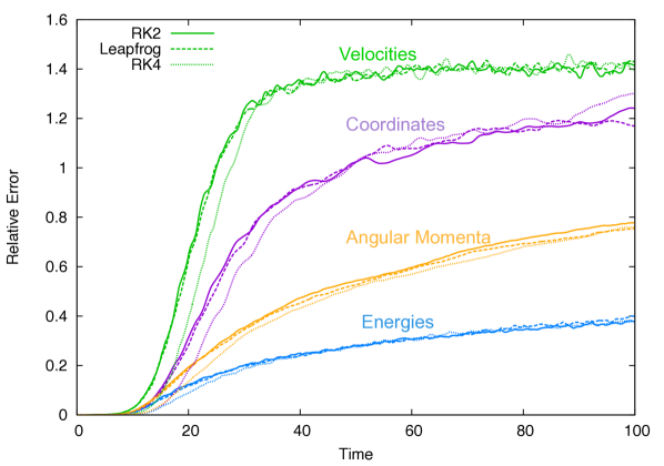
Figure 11: Comparison of error growth in leapfrog, second order Runge-Kutta (RK2) and fourth order Runge-Kutta (RK4), with fixed stepsize. The errors are inferred by repeating the runs while halving the stepsize, with $N=2048$.

We would like to estimate the timescale over which the error in a given variable $V$ reaches a threshold $h$ ($V$ can either be a phase space variable or a mean field conserved quantity). During the exponential phase, the growth in $V$ is $\delta V\sim e^{t/t_{e}}\delta V_{0}$, where $\delta V_{0}$ is determined by the value of the error at the start of exponential growth stage. The timescale to reach $h$ is thus $\ln\frac{h}{\delta V_{0}}$. According to the picture presented above (Section 3.2), exponential growth persists until saturation time $t_{c}$, when $e^{t_{c}/t_{e}}\delta x_{0}\sim R/\sqrt{N}$ (where as before $x$ is a spatial Cartesian coordinate). Assuming this same characteristic exponentiation rate for both $V$ and $x$, (as we already found), and that for $t\gg t_{c}$ the divergence can be approximated by a power law in time, one may suppose that (for $t\geq t_{c}$)

$$\delta V\approx\frac{R}{\sqrt{N}}\Bigg{(}1+\Bigg{(}\frac{t-t_{c}}{t_{c}}\Bigg{)}^{s}\Bigg{)}\frac{\delta V_{0}}{\delta x_{0}}.$$ (14)

From Fig. 8, $1\la s\la 2$ for $t\ga 20$, before either diffusion ($s=1/2$) or saturation ($s\rightarrow 0$) sets in (depending on the variable considered). For $t\gg t_{c}$, one expects a threshold $\delta V=h$ to be reached on timescale $t_{\rm relax}\sim t_{c}N^{1/2s}$. Thus, when a diffusion process is eventually dominant one expects, for a large enough threshold, an error growth that is roughly linear in $N$, akin to that deduced from two-body relaxation estimates. On the other hand, for the systematic evolution — characteristic of the error growth in the phase space variables before saturation sets in — one expects the threshold to be reached on timescales scaling as $\sim N^{1/4}$ to $\sim N^{1/2}$.

Fig. 9 shows the ‘relaxation times’, taken to reach thresholds $h=5\%$ and $h=33\%$. The timescales to reach the $5\%$ threshold are dominated by the early exponential evolution. The exponentiation rates do not vary much with $N$ or variable type. However, the error $\delta V_{0}$ at the start of the exponential period however does, particularly due to the role of strong encounters as described in Sections 3.2.3 and 3.2.4 — hence the dependence on $N$ and variable type. In the case of energy error growth, which as was seen is relatively slow, the associated relaxation time at $h=5\%$ is large enough for the effect of the post-exponential evolution to be dominant for larger values of $N$. The growth of the timescale for the errors to reach $5\%$ is in this case consistent with a scaling $\sim N^{1/4}$ for $N=512$ and larger.

For the threshold of $33\%$, there is clear separation between the relaxation times associated with the different variables. For the energy, a diffusion process is dominant at all $N$, and the relaxation time for error growth to reach $h=33\%$ is roughly linear. Indeed, it follows quite well the two-body relaxation form, with Coulomb logarithm factor $\gamma=0.11$, as suggested by Giersz & Heggie (1994). (Note that the last two points, $N=4096$ and $N=8192$, are missing because the energy error does not reach $33\%$ over the timescales considered). For relatively small $N$ (up to $N=512$), the timescales associated with velocity and angular momentum errors are still dominated by the mechanisms of error growth that affect the angular momentum and velocity in similar manner (the pre-exponential, exponential, and systematic evolution driven by the multiplicative enhancement of encounters discussed in Section 3.2.2). For larger $N$, however, the timescale associated with the velocities grows as $\sim N^{1/4}$ (corresponding to $s\sim 2$ in 14). The angular momentum relaxation to the $33\%$ level, on the other hand, follows roughly a $N^{1/2}$ scaling. Except for the last point, when it steepens significantly as the diffusive contribution finally becomes dominant at $N=8192$.

3.5 Propagation of errors in fixed stepsize integrations

The simulations presented in the previous subsections came with the advantage of an error estimate, calculated from a preset tolerance, which limits the maximal error even in the absence of softening. This is the case where the central contradiction between the persistence of the exponential instability with non-saturating rate and the predictions of the collisionless limit is clearest. The local error, set by the tolerance, could be inserted into theoretical estimates of the dynamics of the growth of errors. It could thus be compared with the global error estimated using the reversibility criterion, which is linked to theoretical measures of dynamical information loss (as discussed in the Appendix).

From a practical numerical point of view however, the method used in the previous subsections may seem detached from modern $N$-body simulations of collisionless systems. For these normally use symplectic methods, which are time symmetric and therefore reversible when the dynamical equations are. The criterion of reversibility then becomes evidently irrelevant (except for tracking roundoff error if floating-point arithmetic is used). Simulations intended to model collisionless systems also invoke softening of the gravitational force.

In this section, we repeat all our simulations while using a leapfrog integrator with fixed stepsize and softened force law. We run pairs of simulations, such that for every run there is an auxiliary one with the stepsize halved. An error estimate is derived by comparing the trajectories of the simulations with the larger stepsize with those with the smaller ones (started with exactly the same initial conditions). For our fiducial runs, we set the larger timestep at $\Delta t=10^{-2}$ units and the (Plummer) softening to $\epsilon^{2}=0.001$. For these values, the softening is small enough so as not to drastically suppress the dynamics of the exponential growth, and the RMS errors in particle energies are approximately the same as in the runs of the previous subsections. We have not undertaken a comprehensive examination of the effects of varying the softening and stepsize. However some trials — in the range of $10^{-4}\leq\Delta t\leq 10^{-2}$ and $\times 10^{-5}\leq\epsilon^{2}\leq\times 10^{-3}$ — suggest that the qualitative behaviour described below is generic. Though the absolute numerical values of error growth rates in each variable are sensitive to $\Delta t$ and $\epsilon$, the relative growth rates in the different variables (coordinates, velocities, energies and momenta) are similar.

Some of the results are shown in Fig. 10. For the largest $N$ runs ($N=8192$), they are qualitatively the same as those in the corresponding Fig. 7. Except for the slower initial growth, due to the presence of softening, they are also quantitatively similar. Some differences are however apparent between the smaller $N$ runs. First, there is a steeper rise in the post-exponential error growth curves of the phase space variables, particularly the positions. In the light of the tests we have conducted (and describe further below), this is probably due to the lack of error control, provided in the previous subsections by the preset tolerance. This leads to faster growth of errors in the phase space variables in the present runs, as compared to what was found before. If one assumes that encounters leading to growth of errors are local, and thus initially affect only the velocities, then the larger errors in positions would reflect inter-encounter enhancement of errors initiated at discrete encounters. These would be mainly errors in phases of trajectories, which would explain the especially steep error growth, in both phase space variables, when phase mixing is the dominant mechanism of growth, immediately prior to saturation. More importantly, Fig. 10 also shows slower initial rise in the angular momentum errors, and a clearer transition to the diffusion limit than found in Fig. 7, where an adaptive stepsize was used in conjunction with a preset tolerance. For smaller $N$, that prescription thus seems to enhance the error growth in angular momentum during the systematic growth stage, and to suppress its subsequent diffusive evolution.

Figure 12: Error growth evaluated using a fixed stepsize fourth order Runge-Kutta method and employing the reversibility criterion. With (Plummer) softening $\epsilon^{2}=0.001$ (left panel) and $\epsilon^{2}=0.00025$ (right panel), and $N=2048$.

Figure 13: ‘Relaxation times’, determined by evaluating differences between full and half timestep trajectories at the $33\%$ (left panel) and $66\%$ (right panel) threshold levels. At the $33\%$ error level, the energy relaxation can still approximately follows the two-body relaxation form with the same parameters as in Fig. 9. The velocity error $N$-scaling is also similar at this threshold. The angular momentum relaxation $N$-scaling is however different. Due to slower error growth, it no longer closely follows that of the velocities at smaller $N$, and the parametrisation used in Fig. 9 for larger $N$ (reproduced here for comparison), no longer provides an adequate approximation. Nevertheless, the diffusion limit, and associated ’two-body scaling’, is only reached for the relatively high error threshold of $66\%$.

In addition to checking that this general behaviour does not depend on $\Delta t$ and $\epsilon$ — at least in the range mentioned above — we have checked that it persists when the smaller stepsize is reduced down to a tenth of the larger one (instead of half). We also confirmed that it is not due to any structural evolution during the forward runs when the reversibility criterion is used. This was done by running the systems for 100 (and 200 and 300) units before halving the timestep and comparing the evolution with full and half stepsizes.

The differences are also not due to the use of the symplectic leapfrog integrator. This can be seen from Fig. 11, where we present a comparison with what is obtained when a fixed stepsize second and fourth order Runge-Kutta are employed. The error growth associated with the second order Runge-Kutta is almost identical to the leapfrog, while the fourth order is somewhat smaller in magnitude, but still qualitatively similar for all variables. Thus, at least in terms of error propagation as measured here, it would appear that the advantage of the leapfrog method is confined to it being less expensive; needing one force evaluation per timestep instead of two for second order Runge-Kutta or four (for fourth order).

As a final test, we checked whether the discrepancies are related to the different error measures used; namely, comparing systems integrated with different stepsize, as done in this section, as opposed to comparing the forward and reversed in time systems, as done previously. In Fig. 12 we present the results of a comparison run, using the reversibility criterion of the previous subsections but in conjunction with a fourth order Runge-Kutta with fixed stepsize. Although the error growth is initially somewhat smaller in magnitude (compared to the lower left hand panel of Fig. 10 and the RK4 curves in Fig. 11), the qualitative behaviour is the same. The quantitative differences can moreover be largely eliminated by varying the stepsize or the softening (as the right hand panel plot suggests). The differences with results of the previous subsections are thus not due to the different error measures used.

It is therefore apparent that the slow error growth rate in momenta at smaller $N$, relative to other variables considered, is due to the use of a fixed stepsize, as opposed to one varied in accordance with a preset tolerance level as in the previous subsections. The energy errors are similar in the two cases (since, by construction, we could choose the timestep and softening so as to ensure this). Since a preset tolerance, has limiting the maximum error in the phase space variables as criterion, it naturally limits the growth in these. However, the control of errors in the phase space variables does not seem to reflect into a corresponding decrease in the angular momentum errors, at least in the systematic growth stage, when it is actually enhanced for smaller $N$. In the diffusive stage, when it seems suppressed, the previous accumulation of errors is such that, when this stage is reached, the errors added are not large enough to become immediately apparent, except for $N=8192$ or near the very end of the runs (as can be inferred for example from Fig. 8). In the fixed stepsize runs presented here, on the other hand, the pre-difussive error propagation is less steep and the diffusive growth is large enough to be measured as it sets in, even in the smaller $N$ runs.

As the angular momentum error growth in the simulations presented here displays clear diffusive evolution, like the energy, we may expect an associated two body relaxation $N$-scaling, as previously found for the energy (Fig. 9, right panel). Even if this should occur for a larger error threshold, as the errors in angular momentum are still clearly larger than those in energy. This is examined in Fig. 13. For a $33\%$ threshold, the energy errors still scale as in Fig. 9. For this error threshold, the velocities also scale approximately as before. However, the $N$-scaling of the angular momentum errors is steeper than in Fig. 9. The parametrisations used there (and reproduced for comparison) is no longer adequate. But the scaling is still slower than that characteristic of two body relaxation. For a $66\%$ threshold, the velocity errors still vary relatively weakly with $N$, while the angular momentum errors now follow the same two body relaxation form that the energy errors followed at the $33\%$ threshold. Thus, as in the case of energy, a clear transition from systematic to diffusive growth is finally detected. But the systematic stage of error growth still dominates till the errors are about twice those in the case of energy. The faster error growth in angular momentum implies that the timescales to reach that larger error threshold are similar for the energy errors to reach the $33\%$ threshold. Assuming diffusive growth, a threshold larger by factor of two, reached on the same timescale, translates to a ‘relaxation time’ that is smaller by a factor of four.

3.6 Summary and discussion

There are three qualitatively different ways through which errors in the trajectories of $N$-body systems can grow. They can grow systematically, as linear or polynomial functions in the number of time-steps $n$; or they can undergo a random walk and grow diffusively (as $n^{1/2}$); or they can grow exponentially. Through examining the numerical reversibility of spherical $N$-body systems, we have observed three stages of error growth incorporating these different aspects. Through the first two stages, the error growth is similar for the phase space variables (coordinates and velocities) and the mean field conserved quantities (energies and angular momenta), while the third stage is characterized by different modes of growth for the two types of variables. The difference becomes apparent once the ‘chaos’ of the exponential instability has saturated, and the subsequent systematic growth, associated with the same sort of coherent scattering that lead to the exponential instability, has subsisted. The error in the phase space variables can then grow by phase mixing, while that of the mean field conserved quantities grows through a diffusion process.

The initial stage occurs over timescales smaller than the exponential divergence timescale. The errors involved are principally truncation errors enhanced by strong encounters. This phase sets the initial errors that are inflated in the subsequent exponential stage. The results of a theoretical model of the error growth through these two stages are shown in Fig. 5. The characteristic exponential timescale implied is a fraction of a dynamical time ( corresponding to $0.15~{}t_{D}(r=a)$ and $0.08~{}t_{D}(R_{v})$). The error inferred from comparison of the forward and reverse dynamics is compatible to those estimated by the Runge-Kutta routine for relatively large $N$ but are much larger than these for smaller $N$. We interpret this in terms of the role of strong encounters, which diminishes as $N$ increases.

The exponential growth in coordinate errors does not saturate at dimensions comparable to the system size (as in systems where ‘chaos’ can lead to global structural evolution); in fact, it already effectively ceases as the distance between two initially nearby trajectories becomes of order $1/\sqrt{N}$ the characteristic system size. We adapt a model due to GHH to interpret this phenomenon. In its context, the theoretical (dashed) lines of Fig. 3 show that the coherent, multiplicative enhancement of errors due to encounters, that leads to exponential divergence, persists even after the saturation of the exponential growth. In fact up to when the effective exponential rate is $\la 10\%$ its initial flat value. This implies that the systematic post-exponential evolution of the errors in the phase space variables is not immediately dominated by phase mixing, and neither is the post-exponential growth of errors in the mean field conserved quantities immediately diffusive. For angular momentum, diffusive growth in fact only becomes apparent at larger $N$ and late times when an adaptive timestep is used (cf. Fig. 7). The growth of energy errors on the other hand always clearly displays diffusive behaviour, with growth rate $\sim t^{1/2}$, after about ten dynamical times. In contrast, the post-exponential evolution of the errors in the phase space variables can be locally characterised by a power law time evolution with index $1\la s\la 2$.

The different modes of error growth lead to different estimates of the associated ‘relaxation times’ — that is, the time the errors in a given variable reach a certain fixed relative error level. For small thresholds (e.g., $5\%$), the errors are dominated by the early growth. The relaxation times are very similar for the velocity and angular momentum, and also for the energy at lower $N$. At higher threshold (e.g. $33\%$ level) the energy error growth is already fully diffusive, its $N$ variation is nearly linear and well explained by a two-body relaxation law with Coulomb logarithm $\gamma=0.11$. Assuming that error growth continues diffusively to the $100\%$ level, the error growth time to this level is $t_{\rm relax}=0.26~{}\frac{N}{\ln(0.11N)}~{}t_{D}~{}(R_{v})$. This is quite similar to standard estimates of the two-body relaxation time.

As the velocity perturbations do not grow diffusively, the associated relaxation time has weaker $N$-scaling even at the $33\%$ error threshold. And since angular momentum error growth initially follows that of the velocities, its relaxation time is also characterised by weak $N$-scaling. When a fixed stepsize is used, however, convergence of angular momentum errors to the diffusive limit is easier to identify. This is the case both when a symplectic (leapfrog) or fixed timestep Runge-Kutta methods are employed. In general, the results are almost identical (Fig. 11). Tests we have conducted however suggest that a preset tolerance level controls the errors in the phase space variables in a way that does not translate into a similar decrease in errors in the mean field conserved quantities, especially for smaller $N$. For the same energy errors, the angular momentum errors are generally smaller in the fixed stepsize runs, while those in the phase space variables are larger.

Still, even in the case of the fixed stepsize runs, the diffusion limit in angular momentum is reached at a larger threshold than in the case of energy. The corresponding relaxation time is about four times smaller. This accelerated relaxation rate may affect the structure of simulated objects, particularly velocity anisotropies. It may also affect the spatial symmetry of triaxial systems, if the strong error growth in angular momentum extends to general action variables of regular orbits; in configurations with a mixed phase space of regular and chaotic orbits in the collisionless limit, regular trajectories may diffuse into chaotic regions at a rate that is larger than that expected from standard two body relaxation estimates, thus accelerating morphological evolution. Such effects may be particularly important in small haloes and subhaloes, which are identified in cosmological simulations with relatively small number of particles, and far larger errors in force calculations and time integration than in the simulations presented here.

Even in the case of energy, slow diffusive error growth is only reached for relatively large error threshold (already at $33\%$, in the simulations presented here). And the $N$-scaling of the errors can be far slower than the expected two body scaling until the diffusion threshold is reached. This suggests that though there is convergence to the collisionless limit in a formal sense, which is important from the theoretical point of view, as discussed below, this convergence is slow.

4 Chaos and collisionless equilibria

In what sense are $N$-body gravitational systems ‘chaotic’? Generally, one can identify chaos with the presence of a positive Lyapunov exponent. The exponential divergence between nearby trajectories does imply the existence of at least one ‘finite time’ positive exponent (strictly speaking, the exponents involve an infinite time limit, which is not well defined for systems with non-compact phase space as $N$-body systems). Furthermore, for unsoftened systems, the associated timescale does not increase with $N$, and in that sense the instability does not saturate. For configurations with smoothed out potentials that are integrable, this directly contradicts the predictions of the collisionless limit, where all orbits are regular. Nevertheless, the results of the previous section confirm that this instability does not imply global structural evolution on the associated timescale, as it saturates on progressively smaller scales as $N$ increases. And mean field conserved quantities, such as energy and angular momentum, eventually evolve via a standard diffusive process. So in what formal sense are these systems chaotic; and does it matter, from a physical point of view?

A key issue concerns information loss, reflected in the numerical irreversibility and error propagation observed in the previous section, and whether it actually affects macroscopic parameters (spatial density, velocity dispersion etc.), describing the gross statistical properties of the system (represented by moments of the one particle distribution function in case of collisionless systems). In terms of numerical implications, if the local instability of trajectories affects the numerical image of systems whose physical properties should remain unaffected by the instability, then it degrades the faithfulness of simulations as well as their accuracy.

To reconcile the fact of positive Lyapunov exponent with apparent lack of macroscopic evolution on the characteristic timescale, one should show that the associated loss of information decreases with $N$ at any macroscopic scale, and that it leaves the statistical quantities characterising macroscopic structure largely unaffected. For this purpose, one can make use of the phenomenon of the saturation of the exponential instability on progressively smaller scales, by relating it to a measure of information loss on the phase space variables and conserved quantities. The concept of dynamical information loss can be made precise through the Kolmogorov entropy, which essentially measures the rate of increase in the information needed to follow a phase space trajectory in time (e.g. Lichtenberg & Lieberman 1992). A formal definition is technically involved, and a discussion as how it can be applied to $N$-body systems, showing its close connection to effective irreversibility, is relegated to the Appendix. Here we use a simpler definition based on the growth of coarse grained phase space volume.

Let $\Omega(0)$ represent a volume in a six dimensional phase space of positions and velocities. Assume that $\Omega(0)$ is occupied by a continuous distribution of phase points, which define a set of initial conditions at a time $t_{0}$ (for finite $N$-systems, this implicitly assumes a statistical ensemble of such systems, similar to the average over simulations presented earlier, but as the number of ensemble members increases arbitrarily). If the phase space is discretised into cells of volume $\Delta\Omega$, then $\Omega(0)$ is obtained by counting the number of cells that the phase points occupy. Even if a subsequent dynamical evolution of the phase flow obeys the collisionless Boltzmann equation — and so Liouville’s theorem applies on the 6-d phase space — after $n$ timeteps, the volume on the coarse grid will evolve such that $\Omega(n)\geq\Omega(0)$, as trajectories initially confined to a single cell at time $t_{0}$ can spread over many cells at later times. In terms of the standard Boltzmann entropy, $\log\Omega(n)$, one can then define

$$K(\Delta\Omega)=\lim_{n\rightarrow\infty}\frac{1}{n}\log\frac{\Omega(n)}{\Omega(0)},$$ (15)

which is non-vanishing if the volume increases exponentially. The Kolmogorov entropy proper is the limit of $K(\Delta\Omega)$ as $\Delta\Omega\rightarrow 0$.  A nonzero value is associated with the presence of positive Lyapunov exponents (and is directly related to their sum; e.g., Lichtenberg & Lieberman 1992). In this sense, due to the exponential divergence at infinitesimal scales, $N$-body systems have positive Kolmogorov entropy that does not decrease with $N$, as the exponentiation rate does not. 

Nevertheless, the scale saturation of the exponential divergence implies that, at any finite volume resolution $\Delta\Omega$, $K=0$ as $N\rightarrow\infty$. For, given any two initially infinitesimally nearby trajectories and characteristic system size $R$, there is a maximal spatial distance $\sim R/\sqrt{N}$ (with corresponding maximal difference in velocities), beyond which they cannot separate by means of the exponential divergence. And if the progressively smaller scales over which the exponential instability occurs are not resolved, the exponential growth cannot be detected. As the maximal volume in which the location of a phase space point is uncertain at the conclusion of the exponential stage decreases (as $\sim 1/N^{3}$), so does the information loss suffered at the completion of that stage. For an initial uncertainty $\Delta x$ in phase space coordinates, it goes as $\log\left(\frac{R}{\Delta x\sqrt{N}}\right)^{6}$. Eventually, in any numerical implementation, there is a maximal resolution imposed by machine precision. Thus, in principle, beyond $R/\sqrt{N}\sim 10^{-14}$ there would be no meaning for ‘chaos’ due to the exponential instability, as far as double precision numerical implementation is concerned.

The argument above is general. It concerns the loss of information due to the intrinsic exponential divergence of $N$-body systems and the scales on which it acts. This instability is invariably present at these scales, with the same timescale of a fraction of a dynamical time, regardless of the gross structure of the $N$-body configuration. After it saturates, however, the further growth of errors will depend on the detailed dynamics of the system at hand, for example on the spatial symmetry of the smoothed potential and whether it is time dependent or not. As the saturation occurs on smaller scales with larger $N$, this further growth of errors, which we now discuss, becomes increasingly important. The arguments below pertain particularly to configurations in dynamical equilibrium and which support only regular orbits in the collisionless limit, and are thus characterised by distribution functions that depend only on integrals of motion of these orbits. This special case is the basis of much of classical galactic dynamics. In its context, the loss of information is limited, quantitatively and qualitatively, by the slow post-exponential growth of errors, especially by the transition to slow diffusive growth in the mean field conserved quantities (that, is the integrals of motion in the smoothed potential).

Suppose that a set of trajectories (phase points) are started on an energy surface in phase space. As the system evolves, they will remain confined to volumes associated with a narrow energy range $\Delta E(t))$ that eventually grows only on the two body relaxation timescale. For spherical configurations with isotropic velocities, this is a shell with volume that can be expressed in terms of radial coordinates $r$ and $v$ in position and velocity space as

$$\Omega(\Delta E)=\frac{\partial\Omega(E)}{\partial E}\Delta E=(4\pi)^{2}\Delta E\int_{0}^{r_{\rm max(E)}}v(E,r)r^{2}dr,$$ (16)

where $\Omega(E)$ is the phase space volume volume enclosed by energy surface $E$. This scales as $\sim\Delta Evr^{3}$, with $r$ and $v$ understood as typical radial phase space coordinates at energy $E$. Next, consider initial conditions known to be homogeneously distributed within a cell of phase space of volume $\Delta\Omega(0)\sim\Delta v_{0}^{3}\Delta r_{0}^{3}$, where $\Delta r_{0}$ and $\Delta v_{0}$ are uncertainties arising from coarse graining. Due to the loss of information associated with the dynamics, the phase point locations will eventually, after a time $t_{E}$ say, be uncertain. As we saw in the previous section, the error growth rate in energy is much smaller than that in angular momentum. One may then consider an intermediate state when the phase points would be uncertain only within the energy shell $\Delta E$, even after loss of information on other mean field conserved quantities is essentially complete. In this case, the location of the phase points will be uncertain within a volume $\Delta\Omega(t_{E})=\Omega(\Delta E)$, which is $\sim\Delta Evr^{3}$. If initially $\Delta E_{0}\sim(\Delta v_{0})^{2}$, then assuming strict energy conservation ($\Delta E=\Delta E_{0}$), but complete loss of information on the location of phase space points within the energy shell, implies

$$\frac{\Delta\Omega(t_{E})}{\Delta\Omega(0)}\sim\frac{vr^{3}}{\Delta v_{0}(\Delta r_{0})^{3}}.$$ (17)

If $\Delta v_{0}/v=\Delta r_{0}/r\sim 10^{-14}$, say, then $\Delta\Omega(t_{E})/\Delta\Omega(0)\sim 10^{56}$. Thus, the exponential instability, which seeds the process of loss of information over the energy shell, does have an effect in this sense. However, although the volume multiplication is large, the timescale over which it occurs increases with $N$, since for large enough $N$ most error accumulation occurs after the saturation of the exponential instability. According to estimates of Section 3.4, the timescale associated with the error growth in the phase space variables should then scale as $N^{1/4}-N^{1/2}$. Furthermore, even with total uncertainty on the phase space variables within the energy shell, the loss of information is still quite small compared to that accompanying an energy uncertainty also of order one, in which case an additional factor of $10^{28}$ in volume ratio is involved. And this last process occurs over the still longer timescale of diffusive error growth, scaling as $\sim N$.

More importantly, information loss that occurs while the integrals of motion remain well conserved primarily reflects uncertainty in the phases of trajectories. It is in this sense dynamically trivial, and its implication concerning simulated systems relates to the accuracy of the results and much less to the faithfulness of the representation. For example, suppose the system (as is the case of the systems considered in the previous section), can be characterised by a distribution function $f=f(E)$. As long as energies are reasonably well conserved along trajectories, even total loss of information on the phase space coordinates does not imply corresponding evolution in the distribution function. Hence it should not significantly affect the macroscopic state of the self gravitating configuration, described by $f$ and its moments. Indeed, if phase points were labelled only by their energies, and the phase space coarse-graining done solely in terms of energy shells $\Delta E$, then the coarse grained $\Omega(\Delta E)$ would not change dramatically over timescales much smaller than the energy relaxation time. The entropy given by equation (15) would still be non-zero over infinitesimal scales, as on these scales the exponential divergence affects the mean field conserved quantities in the same manner as the phase space variables. But after it saturates, the information loss is limited, as the slow diffusive stage of error growth is reached. A similar situation would arise if the distribution function depended also on momenta, $f=f(E,L)$, or was a function of action variables in the case of general integrable potentials.

To sum up. For any finite phase space resolution, the Kolmogorov entropy tends to zero as $N\rightarrow\infty$. In particular, for any spatial resolution $\ga R/\sqrt{N}$ it tends to zero. The information loss incurred during the exponential stage is thus increasingly limited with increasing $N$, as its saturation scale shrinks. From this perspective, the exponential instability in large $N$-body systems does not imply that they undergo significant ’chaotic mixing’, which explains why they do not generally display relaxation and evolution of macroscopic quantities on the exponential timescale, a characteristic of systems where the exponential instability saturates on larger scales (Kandrup & Sideris 2003). Second, although dynamical evolution leads to large loss in information regarding the phase space coordinates of trajectories, beyond the exponential regime this occurs on timescales that increase with $N$. The loss is moreover small compared to that accompanying the error growth in the mean field conserved quantities, which takes place on a still longer time scale with steeper $N$-scaling, akin to that of standard two body relaxation. Thus, for systems characterised by a distribution function that depends on the mean field conserved quantities, the the gross structure is largely unaffected on smaller timescales, despite the large loss of information on the phase space coordinates of trajectories.

This gives confidence in the convergence towards the collisionless limit and its predictions, despite the persistence of the exponential instability on infinitesimal scales. It gives credibility to the practice of modelling gravitational systems through orbital integration in smooth potentials — the process of mapping characteristics curves of the collisionless Boltzmann equation — and credence in the faithfulness of $N$-body simulations, despite the loss of information inherent in numerical integration. It should be noted nevertheless that the slow scale saturation of the exponential stage — which is followed by systematic growth of errors before slow diffusion sets in, even in the case of the mean field conserved quantities — points to the slowness of the convergence. Indeed, as we saw in the previous section, the diffusion limit, and associated steep $N$ scaling for error growth, was only reached at the $33\%$ error threshold in the case of energy. This threshold was even larger in the case of angular momentum (indeed, in this case, the diffusion limit was clearly reached at all, for all $N$, only in the fixed timestep runs).

5 Conclusion

We have examined two related aspects of $N$-body gravitational systems; the dynamical divergence of initially nearby solutions and the faithfulness of their numerical simulations. We did this by considering the simple case of spherical systems in dynamical equilibrium, running a suite of small $N$ but high accuracy simulations, in the range of $N=128$ to $N=8196$, while quantifying the direct consequences of the growth of errors. This was done by studying the numerical reversibility of solutions advanced with a preset error tolerance (set to $10^{-8}$), and also by comparing fixed timestep integrations conducted with different stepsizes. The latter method mainly employed the widely used symplectic leapfrog integrator, with some comparison runs using second and fourth order Runge-Kutta. The force law was softened, as opposed to the case in runs with adaptive stepsize, where there was no softening.

Three phases of error growth can be distinguished. A simple calculation and numerical results show that the errors add up randomly before the well known local exponential instability of $N$-body systems sets in. As have been found in other studies, the exponential growth time is virtually independent of $N$. However the pre-exponential growth is sensitive to $N$; as measured by the irreversibility of the computed dynamics, it is larger than the estimated truncation error for relatively small $N$ but significantly smaller than that error for larger $N$. Moreover, the exponential instability saturates at progressively smaller spatial scales, of order $1/\sqrt{N}$ the system size, as $N$ increases. A simple model, originally due to Goodman, Heggie & Hut (1993), was adapted to study this phenomenon quantitatively.

These first two phases of the error growth set the stage for the third phase, by providing its initial conditions. This stage starts with systematic growth, driven by the same mechanism of coherent, multiplicatively reinforcing enhancements, born of encounters of the same sort that lead to the exponential instability. Subsequent to this, the growth of errors is qualitatively different in the case of the phase space variables (coordinates and velocities) and the conserved quantities of the mean field dynamics (energies and angular momenta); the former grow through phase mixing, while the latter grow according to a diffusion ($\sim t^{1/2}$) law. This implies different timescales for error growth and their variation with $N$.

The convergence towards the diffusion limit is always clear in the case of energy, where the inferred ‘relaxation time’ of error growth is of the form of that obtained from standard two-body relaxation theory. The convergence towards that limit is harder to identify in the case of angular momenta, especially when a variable timestep is used. In this case, for a similar level of energy errors, the preset tolerance level limits the error growth in the phase space variables in a way that does not translate into similar control in angular momentum errors, especially for smaller $N$ (for larger $N$, there is general agreement with the results of the fixed stepsize runs). Even in the case of the fixed stepsize runs however, the diffusion limit in angular momentum is reached only at an error threshold about double that of energy (and already when the relative error has reached $66\%$).

The relatively short angular momentum error growth times may have consequences for estimating the effect of discreteness effects in simulations. Velocity anisotropies may be particularly affected by the larger growth rate of angular momentum errors, and if the phenomenon applies to general action variables in non-spherical potentials, associated errors can affect the shapes of the corresponding objects (presumably rendering them more spherical). A case in point concerns finite-$N$ configurations with mixed phase space, supporting chaotic as well as regular orbits in the collisionless limit. Here, regular trajectories may diffuse into chaotic regions on timescales shorter than that expected from standard two body relaxation estimates. Once in such regions, the action variables may not be even approximately conserved or defined, and the trajectories may fill the available chaotic region of phase space on a smaller timescales still. Other situations of interest include those involving time dependence of the potential. When this is slow, action variables become adiabatic invariants. The level to which they may be conserved in finite-$N$ systems may also be affected by relatively rapid error growth rates. Such situations, as well more general ones (for example when mergers are involved), may be worth examining in detail in future studies.

The exponential instability persists, at the infinitesimal level, with a rate that does not decrease with $N$. In this sense, arbitrarily large-$N$ unsoftened gravitational systems are ‘chaotic’ even for configurations that support only regular orbits in the collisionless limit. However, when the effect of the local instability is viewed in terms of information loss on a finite resolution scale, a different picture emerges. Because the exponential divergence saturates at increasingly smaller scales, the Kolmogorov entropy, which must be positive for a chaotic system, tends to zero at at any non-infinitesimal resolution level as $N\rightarrow\infty$. This is because, following the completion of the exponential divergence, the volume in which a phase space trajectory can be localised, stage decreases as $\sim 1/N^{3}$. A finite resolution level is inherent in any practical representation, which is ultimately limited by machine precision (or by softening, which, when large enough, has been shown to increase the exponential timescale as $N$ increases: e.g. GHH; El-Zant 2002). This necessarily limits the sense in which $N$-body systems can be termed ‘chaotic’. Indeed, the loss of information is especially minimal if it is viewed in terms of mean field conserved quantities. As long as these are reasonably well conserved a distribution function depending on integrals of motion is also correspondingly conserved, and the dynamics tends to its mean field counterpart, despite the persistence of the exponential instability on infinitesimal scales.

Thus, despite the persistence of the exponential instability — which for spherical systems in equilibrium is in apparent, direct contraction to what is expected in the collisionless limit — our results support the standard assumptions of galactic dynamics, based on that limit. They give credence to the associated practice of modelling large-$N$ systems through orbital integration in smooth potentials, which is perhaps of increasing importance for understanding of Galactic dynamics in the age of GAIA, and confidence in the faithfulness of $N$-body simulations. Nevertheless, the weak $N$-scaling of the error saturation level of the exponential instability entails a similarly weak scaling ($\sim N^{1/4}$ to $\sim N^{1/2}$) for the propagation of errors during the subsequent stage of systematic growth. Even in the case of the mean field conserved quantities, this dominates before the diffusion limit, with its steeper scaling ($\sim N$), is reached. And since this is reached at relatively large error thresholds, the convergence to the predictions of the collisionless limit to high precision (at the $10\%$ error levels say) is slow, even when measured in terms of energy errors. The errors in the phase space variables never reach a diffusive stage; they continue to propagate systematically through phase mixing, and retain a weak $N$ scaling for all error thresholds.

Appendix A Kolmogorov entropy and effective ireversibility

Assume we are dealing with timescales that are small compared to the energy relaxation time, and that the system is described by a 6-d probability phase space distribution function $f=f(E)$ obeying the collisionless Boltzmann equation (and so $f$ is constant along particle trajectories). Discretise the phase space into cuboidal cells, each with volume $\Delta\Omega$, and follow the evolution of a particle trajectory from specified initial conditions. Then record the cell number $c_{i}$ at which a trajectory is located at time times $t_{i}$, with $i=1,..,n$. The Shannon information entropy of this partition of cells under the action of the trajectory is

$$S=-\sum_{i}^{n}p_{i}\log p_{i},$$ (18)

where probabilities $p_{i}$ are proportional to the time the trajectory spends in cell $i$.

Now consider a group of trajectories initially localised in one of the phase space cells. The Shanon entropy for this system of trajectories generally increases as the system evolves, and is maximized as the probabilities $p_{i}$ equate, so that $p_{i}\rightarrow f(E)$ on all cells. The Kolmogorov entropy distinguishes between any general increase in Shanon entropy (e.g. due to phase mixing) and that associated with exponential instability. For our purposes the concept can be developed as follows.

Suppose that after at time $t_{1}$ we take a distribution $f$ of points over the cuboidal phase space cell $c_{1}$ where our integrated trajectory resides. If we reverse back the trajectories in this cell to time $t_{0}$, the collisionless evolution ensures that the fine grained density $f$ is conserved and the distribution will end up under the reversed dynamics in cell $c_{0,1}$ of same volume as $c_{1}$. If there is no divergence between neighbouring trajectories the shape of the cell is conserved during the evolution, and volume conservation implies that cell $c_{0,1}$ will coincide with $c_{0}$ where they all started. In the presence of divergence however, trajectories reversed from $c_{1}$ may fall in cells other than $c_{0}$. In fact the cell $c_{0,1}$ containing the reversed trajectories will be distorted by the evolution and will in general not be cuboidal anymore. The intersection of $c_{0,1}$ with $c_{0}$ will generally define a cell of smaller volume. The continuation of this procedure for times $t_{2},t_{3}...,t_{n}$ defines progressively smaller cells, determined by the intersections of $c_{0,1},c_{0,2},...,c_{0,n}$ with $c_{0}$. Now if we label the cells defined by these intersections as $d_{j}$ (with $j=1,..,n$), and repeat the process for different trajectories of the system (with initial conditions sampled from the distribution function $f(E)$), we can define a finer partition of the phase space. The associated probabilities $p_{d_{j}}$ (which are proportional to $f(E)$ integrated over smaller and smaller volumes of the intersection cells), decrease with increasing maximal timestep $n$.

The Kolmogorov entropy measures the increase per time-step of the Shannon information entropy of this increasingly finer partition as volume $\Delta\Omega$ and the time-step $\Delta t$ both go to zero. This corresponds to the loss of information per time-step, which leads in practice to the inability to numerically track and reverse a trajectory. The reason we obtain finer partitions from the reversed dynamics — and corresponding increase in Shannon entropy — was that trajectories that were initially confined to a cell $c_{i}$ at time $t_{i}$ could be dynamically evolved into occupying many cells (hence the increase in coarse grained volume). This formally relates the phenomenon of effective irreversibility, due to information loss, to the local exponential divergence between nearby trajectories. It also relates the definition here to the more intuitive one given in the body of the paper.

References

- 1974 (1974A&A….37..183A) Aarseth S. J., Henon M., Wielen R., 1974, A&A, 37, 183
- Benhaiem et al. (2018) Benhaiem D., Joyce M., Sylos Labini F., Worrakitpoonpon T., 2018, MNRAS, 473, 2348
- Binney & Tremaine (2008) Binney J., Tremaine S., 2008, Galactic Dynamics. Princeton University Press, Princeton, NJ (BT)
- Blum (2018) Blum A., Hopcroft J., Kannan R., 2018, Foundations of Data Science. https://www.cs.cornell.edu/jeh/book.pdf.
- Braun & Hepp (1977) Braun, W., & Hepp, K. 1977, Communications in Mathematical Physics, 56, 101
- Contopoulos (2002) Contopoulos, G. 2002, Order and chaos in dynamical astronomy /George Contopoulos. Berlin : Springer, c2002. (Astronomy and astrophys library) QB 351 .K58 2002,
- Dehnen & Read (2011) Dehnen W., Read J. I., 2011, EPJP, 126, 55
- Dehnen (2014) Dehnen, W. 2014, Computational Astrophysics and Cosmology, 1, 1
- Dehnen (2017) Dehnen W., 2017, MNRAS, 472, 1226
- Earn (1994) Earn D. J. D., 1994, LNP, 430, 122
- El-Zant (2002) El-Zant A. A., 2002, MNRAS, 331, 23
- Genel et al. (2018) Genel, S., Bryan, G. L., Springel, V., et al. 2018, arXiv:1807.07084
- Giersz & Heggie (1994) Giersz, M., & Heggie, D. C. 1994, MNRAS, 268, 257
- Goodman, Heggie, & Hut (1993) Goodman J., Heggie D. C., Hut P., 1993, ApJ, 415, 715 (GHH)
- Hairer (2006) Hairer E., Lubich C., Wanner G., 2006, Geometrical Numerical Integration , 2nd edn. Springer-Verlag, Berlin
- Hayes (2003) Hayes W. B., 2003, PhRvL, 90, 054104
- Heggie & Hut (2003) Heggie D., Hut P., 2003, The Gravitational Million-Body Problem: A Multidisciplinary Approach to Star Cluster Dynamics. Cambridge University Press, Cambridge
- Hemsendorf & Merritt (2002) Hemsendorf M., Merritt D., 2002, ApJ, 580, 606
- Hernandez & Bertschinger (2018) Hernandez, D. M., & Bertschinger, E. 2018, MNRAS, 475, 5570
- Hoover& Hoover (2012) Hoover W. G., Hoover C. G., 2012, Time Reversibility, Computer Simulation, Algorithms, Chaos. Advanced Series in Nonlinear Dynamics. World Scientific, Singapore
- Huang, Dubinski, & Carlberg (1993) Huang S., Dubinski J., Carlberg R. G., 1993, ApJ, 404, 73
- Kandrup & Smith (1991) Kandrup H. E., Smith H., Jr., 1991, ApJ, 374, 255
- Kandrup & Sideris (2001) Kandrup H. E., Sideris I. V., 2001, PhRvE, 64, 056209
- Kandrup & Sideris (2003) Kandrup H. E., Sideris I. V., 2003, ApJ, 585, 244
- Keller et al. (2018) Keller B. W., Wadsley J. W., Wang L., Kruijssen J. M. D., 2018, arXiv, arXiv:1803.05445
- Lichtenberg & Lieberman (1992) Lichtenberg A. J., Lieberman M. A., 1992, Regular and Chaotic Dynamics. Springer, Berlin
- Miller (1964) Miller R. H., 1964, ApJ, 140, 250
- Portegies Zwart & Boekholt (2014) Portegies Zwart S., & Boekholt, T. 2014, ApJ, 785, L3
- Press et. al. (2007) Press W. H., Teukoslky S. A. , Vetterling W. T., Flannery B. P., 2007, Numerical Recipes: The Art of Scientific Computing. Cambridge University Press, Cambridge.
- Quinlan & Tremaine (1992) Quinlan, G. D., & Tremaine, S. 1992, MNRAS, 259, 505
- Sagdeev, Usikov, & Zaslavsky (1988) Sagdeev R. Z., Usikov D. A., Zaslavsky G. M., 1988, Nonlinear physics. From the Pendulum to Turbulence and Chaos. Harwood Academic Publishers, New York.
- Sellwood & Debattista (2009) Sellwood J. A., Debattista V. P., 2009, MNRAS, 398, 1279
- Sideris & Kandrup (2002) Sideris I. V., Kandrup H. E., 2002, PhRvE, 65, 066203
- Springel (2016) Springel V., 2016, SAAS, 43, 251
- Thiébaut et al. (2008) Thiébaut J., Pichon C., Sousbie T., Prunet S., Pogosyan D., 2008, MNRAS, 387, 397
- Valluri & Merritt (2000) Valluri M., Merritt D., 2000, AdSAC, 10, 229
- Wolf et al. (1985) Wolf A., Swift J. B., Swinney H. L., Vastano J. A., 1985, PhyD, 16, 285
- (38) Young L.-S., in Greven A., Keller G., Warnecke G. eds, Entropy. Princeton University Press, Princeton ,NJ