Performance of the strongly constrained and appropriately normed density functional for solid-state materials

Abstract

Constructed to satisfy all known exact constraints and appropriate norms for a semilocal density functional, the strongly constrained and appropriately normed (SCAN) meta-generalized gradient approximation functional has shown early promise for accurately describing the electronic structure of molecules and solids. One open question is how well SCAN predicts the formation energy, a key quantity for describing the thermodynamic stability of solid-state compounds. To answer this question, we perform an extensive benchmark of SCAN by computing the formation energies for a diverse group of nearly one thousand crystalline compounds for which experimental values are known. Due to an enhanced exchange interaction in the covalent bonding regime, SCAN substantially decreases the formation energy errors for strongly-bound compounds, by approximately 50% to 110 meV/atom, as compared to the generalized gradient approximation of Perdew, Burke, and Ernzerhof (PBE). However, for intermetallic compounds, SCAN performs moderately worse than PBE with an increase in formation energy error of approximately 20%, stemming from SCAN’s distinct behavior in the weak bonding regime. The formation energy errors can be further reduced via elemental chemical potential fitting. We find that SCAN leads to significantly more accurate predicted crystal volumes, moderately enhanced magnetism, and mildly improved band gaps as compared to PBE. Overall, SCAN represents a significant improvement in accurately describing the thermodynamics of strongly-bound compounds.

I Introduction

Density functional theory (DFT) Hohenberg and Kohn (1964); Kohn and Sham (1965) is the standard approach for computing the electronic structure of solid-state materials due to an attractive balance between accuracy and computational efficiency in the Kohn-Sham approach. If the underlying exchange-correlation (xc) energy functional $E_{xc}$ were known, in principle DFT would give the exact ground-state properties of any many-electron system. In practice, the exact $E_{xc}$ is unknown and must be approximated. Examples of such approximations are the well-known local density approximation (LDA) and generalized gradient approximation (GGA). Developing improved approximate functionals for DFT is an important challenge for electronic structure theory.

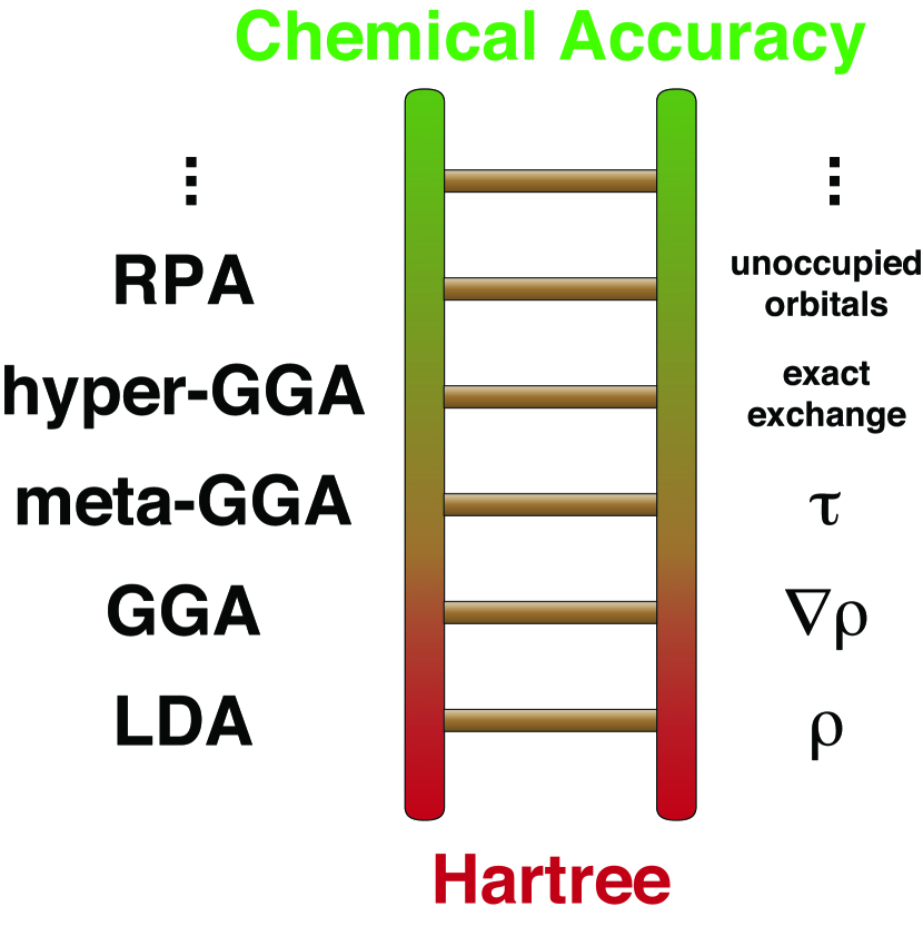
Figure 1: Jacob’s ladder framework for describing different levels of sophistication and accuracy of $E_{xc}$ in density functional theory. Starting from the Hartree level of theory ($E_{xc}=0$) and attempting to climb towards chemical accuracy, each rung of the ladder labeled on the left corresponds to additional dependencies of $E_{xc}$ indicated on the right. The top rung listed is the random phase approximation (RPA). Figure is based on Refs. 3 and 4.

A substantial weakness of DFT is that, unlike certain quantum chemistry approaches, there is no straightforward way to systematically converge to the exact result. In other words, it is not generally clear how to develop increasingly more accurate approximations to $E_{xc}$. However, Perdew has proposed a general framework to describe and develop improvements to $E_{xc}$ by including dependence on additional information. In this framework, known as Jacob’s ladder Perdew and Schmidt (2001), each rung of the ladder is a more sophisticated approximation to $E_{xc}$, as shown in Fig. 1. In the bottom rung, LDA, $E_{xc}$ depends solely the electron density $\rho$. The next rung up is GGA, in which $E_{xc}$ depends on $\nabla\rho$ in addition to $\rho$ itself (for example, in the GGA of Perdew, Burke, and Ernzerhof (PBE) Perdew et al. (1996)). Further up the ladder are more complex $E_{xc}$ functionals containing explicit dependence on Kohn-Sham wavefunctions $\psi$, such as hybrid functionals. While beyond-DFT approaches like DFT+$U$ Himmetoglu et al. (2014) and DFT plus dynamical mean-field theory (DMFT) Kotliar et al. (2006) have not been considered in the Jacob’s ladder framework, they share a similar philosophy. In these methodologies, the energy functional relies on the local density matrix or local Green function, for a set of localized orbitals, in addition to $\rho$, $\nabla\rho$, etc.

Meta-generalized gradient approximation (meta-GGA), the third rung of Jacob’s ladder, takes the $E_{xc}$ form of GGA and adds an additional dependence on the positive orbital kinetic energy density

$$\tau=\sum_{i}\frac{1}{2}|\nabla\psi_{i}|^{2}.$$ (1)

Here $\psi_{i}$ is the Kohn-Sham wavefunction for the $i$th occupied band. $E_{xc}$ now depends on $\tau$ in addition to $\rho$ and $\nabla\rho$:

$$E_{xc}[\rho,\nabla\rho,\tau]=\int\rho\epsilon_{xc}(\rho,\nabla\rho,\tau)\ d^{3}r$$ (2)

Here we consider a spin-dependent meta-GGA, just as the local spin density approximation (LSDA) is the spin-dependent version of LDA. Therefore, just as $E_{xc}$ of LSDA depends on the different spin densities ($\rho_{\uparrow}$ and $\rho_{\downarrow}$) separately, here $E_{xc}$ depends on the different $\rho$, $\nabla\rho$, and $\tau$ for each spin channel. For brevity, we do not indicate the separate spin channels in Eq. 2.

We note that, more generally, the meta-GGA rung of Jacob’s ladder also includes $E_{xc}$ that depends on $\nabla^{2}\rho$ in addition to $\tau$. There is evidence, however, that $\tau$ contains essentially the same information as $\nabla^{2}\rho$ Perdew and Constantin (2007). Therefore, here we only comment on meta-GGA depending solely on $\tau$. $\tau$ is an implicit functional of $\rho$ via the Hohenberg-Kohn theorem. Therefore, meta-GGA can still be considered a pure density functional. Meta-GGA functionals are nonlocal since $\tau$ is not local in $\rho$. However, they can still be considered as semilocal DFT since they are not explicitly nonlocal in $\rho$. Meta-GGA are semilocal in $\psi$. Although nonlocal density functionals (involving a double integral in $\rho$) can be much more computationally intensive, this is not so in the case of meta-GGA since the nonlocality stems only from the dependence on $\psi$, which is readily available.

In 2015, Sun et al. introduced the strongly constrained and appropriately normed (SCAN) functional, a new non-empirical meta-GGA functional Sun et al. (2015). SCAN satisfies all known possible exact constraints for a meta-GGA functional. One example is the requirement that the exchange enhancement factor $F_{x}=E_{x}/E_{x}^{LDA}$ must be no larger than 1.174, a constraint derived from the case of a non-spin-polarized 2-electron density Perdew et al. (2014). Here $E_{x}$ is the exchange part of $E_{xc}$ ($E_{c}$ is the correlation part) and $E_{x}^{LDA}$ is the LDA $E_{x}$. SCAN is also designed to accurately describe particular systems for which exact results are known, which are known as norms. The simplest example of such a norm is the homogeneous electron gas (jellium), which is exactly described by LDA by construction. Examples of norms for SCAN include the jellium surface, as well as the large-$Z$ scaling behavior of the $E_{x}$ and $E_{c}$ for noble gas atoms, where $Z$ is the atomic number. The norms chosen are called appropriate in the sense that a meta-GGA should in principle be able to describe them. Stretched H${}_{2}^{+}$ is an example of an inappropriate norm for meta-GGA since in this case the xc hole will be far from the reference electron Perdew et al. (2016).

The SCAN functional depends on a dimensionless measure of $\tau$ called $\alpha$ defined as:

$$\alpha=\frac{\tau-\tau_{\textrm{single-orbital}}}{\tau_{\textrm{uniform}}}$$ (3)

Here $\tau_{\textrm{single-orbital}}=|\nabla\rho|^{2}/8\rho$ and $\tau_{\textrm{uniform}}=(3/10)(3\pi^{2})^{2/3}\rho^{5/3}$ are the limits of $\tau$ for the single orbital and uniform density cases, respectively. The electron localization function Becke and Edgecombe (1990); Silvi and Savin (1994) can be written very simply in terms of $\alpha$ as $(1+\alpha^{2})^{-1}.$

Figure 2: Non-spin-polarized exchange enhancement factor for the LDA, PBE, and SCAN density functionals as a function of dimensionless density gradient for different $\alpha$. The SCAN functional is constructed based on 3 different limits of $\alpha$ corresponding to the different bonding regimes indicated.

To illustrate the degree to which SCAN differs from the first two rungs of Jacob’s ladder, in Fig. 2 we plot the non-spin-polarized exchange enhancement factor versus the reduced density gradient $s=|\nabla\rho|/[2(3\pi^{2})^{1/3}\rho^{4/3}]$, for different $\alpha$. SCAN distinguishes between three different bonding regimes: metallic ($\alpha=1$), covalent ($\alpha=0$), and weak ($\alpha\rightarrow\infty$). Interpolation between these limiting values is used for other values of $\alpha$. Just as PBE is built around LDA, SCAN is built around PBE. Therefore, just as the $E_{x}^{PBE}\rightarrow E_{x}^{LDA}$ for $s\rightarrow 0$, in the metallic regime ($\alpha=1$), $E_{x}^{SCAN}\rightarrow E_{x}^{PBE}\rightarrow E_{x}^{LDA}$ for the same limit. However, for not-so-slowly varying densities and/or values of $\alpha$ different from unity, SCAN shows significantly different behavior than PBE and LDA.

A limited amount of benchmarking has been performed on SCAN with respect to solid-state materials. Sun et al. computed the lattice constant mean average error for 20 simple elemental and binary solids and found values of 0.081, 0.059, and 0.016 Å for LDA, PBE, and SCAN, respectively Sun et al. (2015). Tran et al. benchmarked a plethora of functionals at the LDA, GGA, meta-GGA, and hybrid levels of theory Tran et al. (2016). In addition to computing the lattice parameter, cohesive energy, and bulk modulus for 44 strongly-bound elemental and binary solids (e.g. Pd, LiF), the lattice parameter and cohesive/binding energy were computed for 5 weakly-bound solids (e.g. Ne, graphite). For the strongly-bound solids, SCAN was found to have the lowest mean absolute relative errors for all the computed properties as compared to the commonly-used LDA, PBE, revPBE, PBEsol, BLYP, TPSS, and PBE0 functionals. The performance of SCAN for the weakly-bound solids was less impressive on an absolute scale (mean absolute relative error in the cohesive/binding energy of over 55%), but again here SCAN out-performed the other common functionals. Several (though not all Charles and Rondinelli (2016)) other recent studies on small numbers of systems are suggestive that SCAN is a significant improvement over LDA and GGA for solid-state materials Sun et al. (2016); Kitchaev et al. (2016); Tian et al. (2016); Kylänpää et al. (2017); Paul et al. (2017); Yao and Kanai (2017); Zhang et al. (2017); Hinuma et al. (2017); Bokdam et al. (2017).

In the present work, we perform an extensive benchmark of SCAN for a diverse set of over 1,000 solids. We focus on the formation energy, which is a central and widely-used quantity describing the thermodynamic stability of solid compounds. We also present results for crystal volume, magnetism, and band gap. In all cases, we compare SCAN to the GGA (PBE) level of theory. PBE is chosen due to the connection to SCAN as well as its prevalence and popularity dft . We find SCAN performs remarkably well for strongly-bound compounds, with a decrease in the formation energy mean average error of around 50% to 110 meV/atom relative to PBE. For less strongly-bound compounds, i.e. intermetallic compounds, SCAN shows no improvement compared to PBE; in fact, it provides moderately worse (by around 20%) formation energy predictions. The distinct exchange behavior of SCAN in the covalent, metallic, and weak bonding regimes is responsible for such trends. SCAN shows significant improvement in predicted crystal structures. In particular, we find a mean average volume error 40% lower than than of PBE. SCAN provides moderately improved band gap predictions compared to PBE, but it still has much larger errors than fully nonlocal functionals such as hybrid functionals and many-body perturbation theory approaches. Overall, SCAN is a significant advance in describing strongly-bound compounds at a modest increase in computational cost.

II Methodology

II.1 Compound formation energy

We benchmark solid-state thermodynamics via the formation energy

$$\Delta E_{f}=E-\sum_{i}x_{i}\mu_{i}.$$ (4)

Here $E$ is the total energy of a compound containing $x_{i}$ atoms of element $i$, which has an elemental chemical potential of $\mu_{i}$, in the formula unit. For example, for FeS₂, $\Delta E_{f}=E_{FeS_{2}}-\mu_{Fe}-2\mu_{S}$. In this work, all formation energies are normalized to the number of atoms in the compound formula unit. We assume the $PV$ term is small for the solid materials studied here, i.e., $\Delta E_{f}\approx\Delta H_{f}$, where $\Delta H_{f}$ is the formation enthalpy. Therefore, in the text we use $\Delta E_{f}$ and $\Delta H_{f}$ interchangeably.

II.2 Elemental reference states

The elemental chemical potentials $\mu$ correspond to the energy per atom of the pure element in a particular reference state. Here we choose the elemental reference states to best match the experiments since we compare to measured formation energies. These reference states generally correspond to the stable phase at standard conditions Dinsdale (1991), with a few exceptions. In the case of P, $\alpha$ white P is the reference state. Since this phase has a complicated structure with partial occupancy, we choose $\beta$ white P as our reference state Aykol et al. (2017). These two phases have similar structural motifs. Similarly, in the case of B we choose $\alpha$ rhombohedral B rather than $\beta$ rhombohedral B. For elements with diatomic gases as the reference phases, we choose the isolated diatomic molecule as our reference phase. We also consider Xe-containing compounds, for which we choose the isolated Xe atom as the reference state. The full list of elemental reference states is given in the Supporting Information

II.3 Compound selection

We use the Open Quantum Materials Database (OQMD) Saal et al. (2013); Kirklin et al. (2015) to acquire the compound and elemental crystal structures, as well as the tabulated experimental formation energies. The experimental formation energies come from two sources: the Scientific Group Thermodata Europe Solid Substance (SSUB) database Scientific Group Thermodata Europe (1999) and the thermodynamic database of the Thermal Processing Technology Center at Illinois Institute of Technology (IIT) Nash (2013). Unlike SSUB, the IIT database focuses on intermetallic compounds.

We find the set of compounds in the OQMD for which the following criteria are satisfied:

1. Compound does not contain Br or Hg

2. There is an experimental formation energy reported for the corresponding composition

3. The compound is reported in the Inorganic Crystal Structure Database (ICSD) Bergerhoff et al. (1983); Belsky et al. (2002)

Criterion 1 is chosen since Br and Hg are liquids at standard conditions, which are more difficult to model. We note that the experimental formation energies are tabulated by composition, rather than by the precise structure, so criterion 2 does not always uniquely identify a single compound with the composition in the case of polymorphism. Criterion 3 is chosen to pick out the structure most likely to correspond to the experimentally measured formation energy. In the case of multiple distinct structures present in ICSD at the composition, we choose the lowest-energy compound (based on calculations in the OQMD). This ensures only a single compound is associated with each composition with a measured formation energy. 1,793 unique compounds in the OQMD satisfy these criteria .

To reduce computational cost, we choose the compounds whose primitive unit cells contain no more than 10 atoms. This corresponds to 1,000 compounds. The distribution of compounds in terms of number of atoms in the primitive cell is included in the Supporting Information. 912 of the compounds are binary, 87 are ternary, and 1 (CaMg(CO₃)₂) is quaternary. 55 of the 1,000 selected compounds are ignored since either (1) there is a significant discrepancy in different reported experimental formation energies, (2) the magnitude of the experimental formation energy is less than 50 meV/atom, and/or (3) the DFT calculation for the compound or any constituent element failed to converge for one or both of the xc functionals. This leaves 945 total compounds. The rationale for excluding these compounds is discussed in more detail in the Supporting Information. We also include the full list of selected compounds, in addition to information on a few exceptions for compound selection, experimental formation energy values, and experimental volume values.

III Computational Details

DFT calculations are performed using the projector augmented wave (PAW) method Blöchl (1994); Kresse and Joubert (1999) with a 600 eV plane wave cutoff using the Vienna ab initio software package (vasp) Kresse and Hafner (1994, 1993); Kresse and Furthmüller (1996a, b). We employ the recommended vasp 5.2 PBE PAW potentials for all calculations (SCAN and PBE) vas since SCAN PAW potentials do not currently exist. This represents an approximation (albeit a widely-used one) as the recent work of Yao and Kanai showed that the use of PBE potentials for SCAN calculations can lead to differences in certain cases Yao and Kanai (2017). Uniform $\Gamma$-centered Monkhorst-Pack $k$-point meshes Monkhorst and Pack (1976) with $k$-point density of at approximately 700 $k$-points per Å^-3 or greater are chosen. The average number of $k$-points times the number of atoms in the unit cell, another metric of $k$-point density, is approximately 11,300. 1st-order Methfessel-Paxton smearing Methfessel and Paxton (1989) of 0.2 eV is employed for structural relaxations, while total energy calculations use the tetrahedron method with Blöchl corrections Blöchl et al. (1994). The energy and ionic forces are converged to 10^-6 eV and 10^-3 eV/Å, respectively. Spin-polarized calculations with ferromagnetic initialization of 3.5 $\mu_{B}$ per magnetic site are employed for compounds containing Sc–Cu, Y–Ag, Lu–Au, La–Yb, and Ac–No; such initialization is also employed for O₂ to properly capture the triplet ground state. For elements with gaseous reference states, the isolated atom/molecule is computed using a face-centered-cubic cell with 15 Å conventional cell lattice parameter and 50 meV Gaussian smearing. We note that our calculations are performed using tighter convergence parameters than the existing PBE-based calculations in the OQMD.

IV Results and Discussion

IV.1 Formation energy

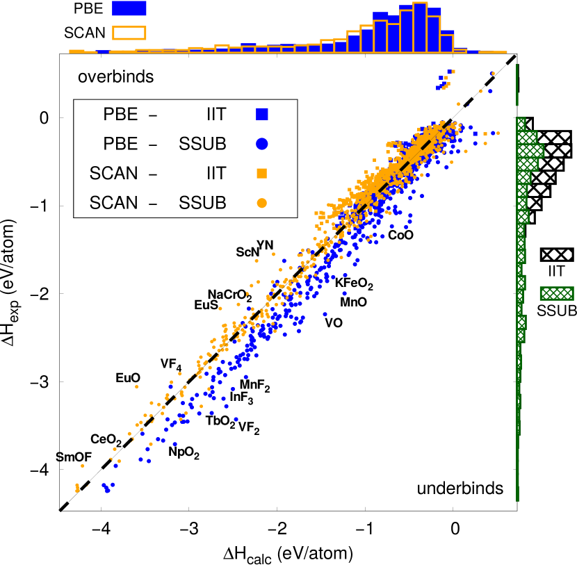
Figure 3: Comparison of calculated and experimental experimental formation energy for the 945 compounds for PBE and SCAN. Multiple points for the same compound and functional correspond to different sources of experimental formation energy. The dashed diagonal line corresponds to the $\Delta H_{calc}=\Delta H_{exp}$ line of perfect agreement. Each bar chart on the axes corresponds to a histogram, which is stacked in the case of the experimental formation energy.

The comparison of computed and experimental formation energies is shown in Fig. 3, which represents the primary result of this work. The most striking trend is the significant improvement of SCAN over PBE for the predicted $\Delta H$ for compounds with a large, negative formation energies. We refer to these compounds as strongly-bound compounds. This trend is seen most dramatically for values of $\Delta H_{exp}$ of around $-1$ to $-4$ eV/atom. Here the magnitude of $\Delta H_{calc}$ for PBE is significantly lower than that of experiment in a systematic fashion, corresponding to an underbinding of the compound with respect to the elements. In stark contrast, no clear systematic underbinding or overbinding of $\Delta H_{calc}$ for SCAN is apparent. We note that the SCAN values for strongly-bound compounds still have deviations (both positive and negative) from the $\Delta H_{calc}=\Delta H_{exp}$ line. A quantitative analysis of the errors, for both functionals, will be presented further below. For compounds with a smaller magnitude of $\Delta H_{exp}$, which we call weakly-bound compounds, the differences in the accuracy of the prediction for PBE and SCAN are less obvious. As shown in the histogram of $\Delta H_{exp}$ in Fig. 3, these weakly-bound compounds represent the majority of the experimental data. This stems in part from the focus of the IIT database on intermetallic compounds, which generally have low-magnitude $\Delta H$.

Figure 4: (a) Absolute and (b) relative errors of the calculated formation energies plotted against the experimental formation energies. The dashed vertical lines correspond to the $\Delta H_{calc}=\Delta H_{exp}$ line of perfect agreement. Histograms of the errors are shown at the top. For the relative errors, the range is limited to $\pm 150\%$.

In order to more easily see the difference in accuracy between $\Delta H_{calc}$ of PBE and SCAN for the full range of $\Delta H_{exp}$, in Fig. 4(a) we plot the error $\Delta H_{calc}-\Delta H_{exp}$ as a function of $\Delta H_{exp}$. Histograms of the errors are also included. Here PBE’s systematic underbinding of $\Delta H$ for strongly-bound compounds can again be observed in the region of $\Delta H_{exp}$ of around $-1$ to $-4$ eV/atom. In addition, the errors appear to increase with increasing magnitude of $\Delta H_{exp}$. In other words, the more negative $\Delta H_{exp}$ is, the more PBE underbinds, which has been previously observed Kirklin et al. (2015). In the histogram of error values for PBE, this systematic underbinding leads to a longer tail of positive error values, resulting in a distribution that appears to be centered around a positive value rather than zero. No such strong systematic underbinding or overbinding for strongly-bound compounds can be observed for SCAN. As such, the distribution of the errors for SCAN appears much better (though not perfectly) centered around zero.

In Fig. 4(a), one can also observe a moderate overbinding trend of SCAN for the weakly-bound compounds. For example, for $\Delta H_{exp}$ of around $-1$ to $-0.5$ eV/atom, many more of the SCAN error values are negative (corresponding to overbinding) than positive. In contrast, such an overbinding tendency for weakly-bound compounds is not observed for PBE. The moderate, systematic overbinding of SCAN for weakly-bound compounds contributes to a slightly negative (overbinding) center-of-mass of the error distribution.

These two trends – SCAN’s lack of systematic underbinding for strongly-bound compounds and its mild overbinding of weakly-bound compounds – are our primary findings in terms of compound formation energy. The same trends can be observed in the relative errors $(\Delta H_{calc}-\Delta H_{exp})/|\Delta H_{exp}|$, shown in Fig. 4(b). Consistent with the absolute error data, PBE exhibits a roughly constant positive average relative error (on the order of +10%) for strongly-bound compounds, contributing to a skewing of the relative error histogram to positive (underbinding) values. In contrast, no clear systematic underbinding or overbinding for strongly-bound compounds is found for SCAN. For the weakly-bound compounds, the relative errors can blow up for compounds with small $\Delta H_{exp}$ due to the $|\Delta H_{exp}|$ in the denominator of the relative error. For example, a relative error of over 240% in magnitude is found for TaCo₂, which has $\Delta H_{exp}$ of only $-0.065$ eV/atom. Therefore, the relative error axis is truncated in Fig. 4(b) for clarity. One can again observe SCAN’s moderate, systematic overbinding of weakly-bound compounds with $\Delta H_{exp}$ of around $-0.5$ to $-1$ eV/atom, contributing to a clear shoulder in the relative error histogram at around $-20$%.

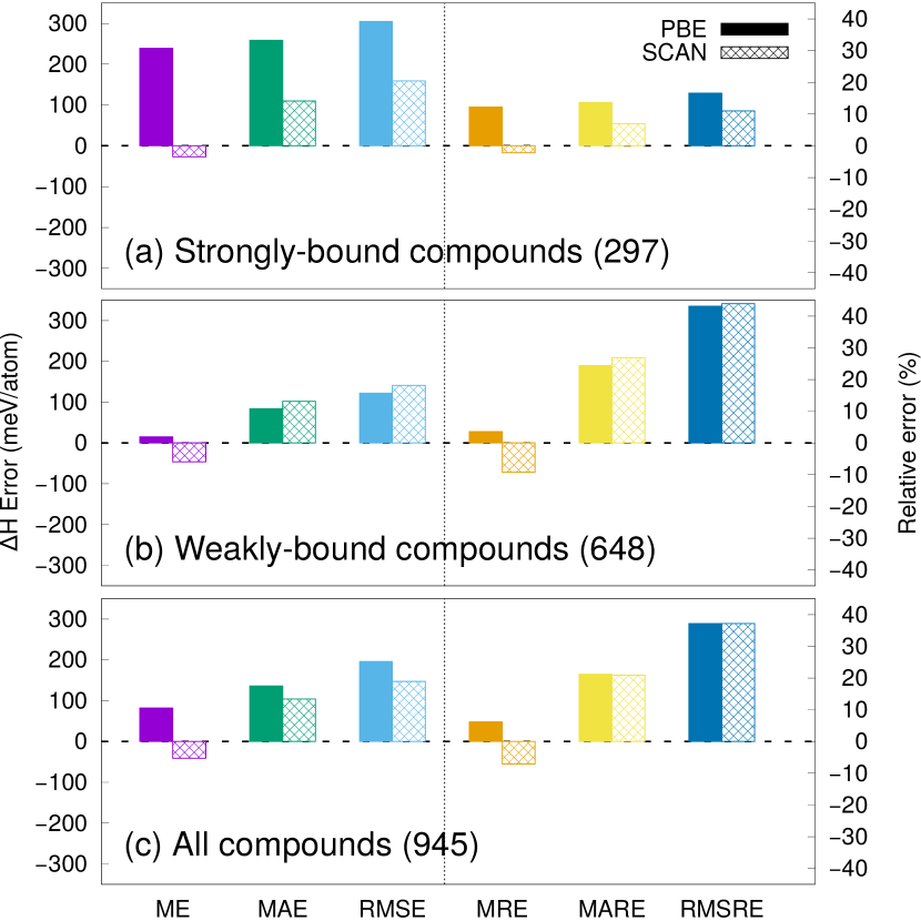
Figure 5: Comparison of absolute and relative errors for PBE and SCAN for (a) 297 strongly-bound compounds, (b) 648 weakly-bound compounds, and (c) all 945 compounds. Absolute (relative) errors are plotted with respect to the left (right) axis.

In order to separately analyze the formation energy errors for strongly- and weakly-bound compounds, we partition the total 945 compounds into these two groups based on $\Delta H_{exp}$. We choose to define strongly-bound compound as any compound with $\Delta H_{exp}<-1$ eV/atom; the rest are weakly-bound compounds. The critical value of precisely $-1$ eV/atom is somewhat arbitrary and is chosen based on visual inspection of the different regions of data in Fig. 3. However, we find no change in the conclusions discussed below by slightly varying this value. In addition, performing an analogous analysis based on partitioning the compound set based on constituent elements rather than $\Delta H_{exp}$, discussed in the Supporting Information, also leads to the same conclusions.

Using this $\Delta H_{exp}$-based convention for compound set partitioning, we quantify the formation energy errors for strongly- and weakly-bound compounds in Figs. 5(a) and 5(b), respectively. Mean error (ME), mean average error (MAE), root-mean-square error (RMSE), mean relative error (MRE), mean absolute relative error (MARE), and root-mean-square relative error (RMSRE) are considered based on the error and relative error expressions discussed above. For each subset of compounds, the absolute and relative error metrics show the same qualitative trend. In particular, by all error metrics SCAN out-performs PBE for the strongly-bound compounds, whereas PBE out-performs SCAN for the weakly-bound compounds. For strongly-bound compounds, SCAN has a ME of only $-0.027$ eV/atom as compared to $+0.239$ eV/atom for PBE. In other words, the distribution of errors for SCAN’s description of strongly-bound compounds is extremely well-centered around zero. This enables much improved MAE and RMSE values for SCAN (0.110 and 0.159 eV/atom) as compared to PBE (0.259 and 0.305 eV/atom). These correspond to very significant ($\approx 50\%$) decreases in error. The maximum absolute error for SCAN ($-0.605$ eV/atom for ScN) is also substantially decreased as compared to that of PBE ($0.963$ eV/atom for VF₂). Similarly large improvements for SCAN are found in terms of the relative errors, with 82%, 49%, and 34% decreases in the magnitudes of the MRE, MARE, and RMSRE values, respectively.

For weakly-bound compounds, we find the opposite qualitative trend. PBE is moderately more accurate than SCAN for such compounds. The ME for PBE is significantly smaller in magnitude ($0.015$ eV/atom) than that of SCAN ($-0.046$ eV/atom). However, SCAN’s increases in MAE and RMSE are a more modest 20% and 16%, respectively, compared to the PBE values. Similarly, for the relative errors, the increase in MARE and RMSRE for SCAN compared to those of PBE are 10% and 2%, respectively. Ultimately, we find SCAN is significantly better for predicting the formation energy of strongly-bound compounds, while it is moderately worse for weakly-bound compounds like intermetallics.

Finally, we briefly comment on the overall $\Delta H_{calc}$ errors (for all 945 compounds). These errors, plotted in Fig. 5(c), reflect the combination of (1) significant error reduction for strongly-bound compounds with large $\Delta H_{exp}$ magnitude and (2) modest error increase for weakly-bound compounds with small $\Delta H_{exp}$ magnitude. In our particular case, there are 648 weakly-bound compounds and only 297 strongly-bound compounds. In this case, SCAN achieves modest decreases in absolute errors with decreases in MAE and RMSE of 24% and 25%, respectively, and essentially no difference in terms of relative errors. We emphasize that the overall formation energy errors in SCAN will be a strong function of the fractions of strongly- and weakly-bound compounds under consideration. Therefore, one should consider the two individual formation energy error trends, rather than the overall trend for our particular compound set, as the key result.

IV.2 Origin of formation energy trends

In order to elucidate the origin of the distinct formation energy trends for strongly- and weakly-bound compounds, we perform a detailed analysis of the strongly-bound oxide CaO and three weakly-bound intermetallic compounds HfOs, ScPt, and VPt₂. While for CaO SCAN reduces the $\Delta H_{calc}$ error from 324 meV/atom in PBE down to just 2 meV/atom, for the intermetallics SCAN increases the error magnitudes by 181–261 meV/atom. We note that both LDA and the earlier meta-GGA of Tao, Perdew, Staroverov, and Scuseria (TPSS) Tao et al. (2003) exhibit similar $\Delta H_{calc}$ as PBE (differences no larger than 19 meV/atom in magnitude) for these intermetallic compounds, which suggests the overbinding of this class of compounds is specific to SCAN.

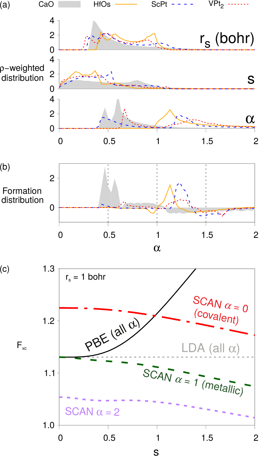
Figure 6: (a) Density-weighted probability distributions of $r_{s}$, $s$, and $\alpha$ in real space for CaO and three intermetallic compounds. The distributions are normalized to unity. (b) The compound $\alpha$ formation distribution defined in analogy to the formation energy of Eq. 4. (c) Non-spin-polarized exchange-correlation enhancement factor at $r_{s}=1$ bohr for LDA, PBE, and SCAN at several relevant $\alpha$ values.

Figure 6(a) contains normalized real-space distributions, for each compound, of the three ingredients to $\epsilon_{xc}$ for SCAN: $\rho$, $s$, and $\alpha$. The density is parametrized by the Wigner-Seitz radius $r_{s}=(3/4\pi\rho)^{1/3}$ for convenience. We weight the distributions by the density $\rho$ since higher-density regions of space have a higher impact on $E_{xc}$ due to the explicit factor of $\rho$ in Eq. 2. The results are shown for SCAN calculations, though we show in the Supporting Information that the distributions are similar for the PBE case.

The distribution of $\alpha$ shows that, unlike CaO, the intermetallic compounds exhibit significant (even dominant in the case of HfOs) probability of larger $\alpha$ in the range of 1–2. In addition, the distributions illustrate the overall relevant ranges of parameter space for the four compounds: $\sim$ 0.25–1.25 for $r_{s}$, $\sim$ 0–1 for $s$, and $\sim$ 0.25–2 for $\alpha$. Including the elemental reference states, whose $\alpha$ and $s$ distributions are shown in the Supporting Information, one finds expanded ranges of $\sim$ 0.25–1.75 for $r_{s}$, $\sim$ 0–2 for $s$, and $\sim$ 0.25–2 for $\alpha$. We note that O₂ has a significantly broader distribution of $s$ and $\alpha$, which is consistent with its distinct molecular nature.

We construct the corresponding formation distribution of $\alpha$ by computing the difference between the $\alpha$ distribution of the compound and the appropriate linear combination of the $\alpha$ distributions of the constituent elements, in analogy to Eq. 4. This function, shown in Fig. 6(b) represents the change in the distribution of $\alpha$ that occurs upon formation of the compound from the elements. The formation distributions show appreciable rearrangement of $\alpha$ upon compound formation. There are distinct behaviors for CaO and for the intermetallics that explain the distinct formation energy behavior for SCAN, which we now will discuss.

The CaO formation distribution exhibits a large positive peak in the vicinity of $\alpha=0.5$, balanced by decreased probability of $\alpha>1$. This peak stems from the filling of the O $p$ shell, whereas the broad valley for larger $\alpha$ corresponds to the depletion of O₂ states. To understand the impact on $E_{xc}$, in Fig. 6(c) we plot the non-spin-polarized exchange-correlation enhancement factor $F_{xc}=E_{xc}/E_{x}^{LDA}$ as a function of $s$ for LDA, PBE, and SCAN for several $\alpha$. As compared to the exchange enhancement in Fig. 2 discussed previously, $F_{xc}$ adds the density-dependent contribution from correlation. The values in Fig. 6(c) are plotted for $r_{s}$ of 1 bohr as a representative example; $F_{xc}$ for other relevant values of $r_{s}$ (shown in the Supporting Information) show the same qualitative behavior. The SCAN $F_{xc}$ increases with decreasing $\alpha$. Therefore, the increased probability for lower $\alpha$ upon formation of CaO leads to a negative $E_{xc}$ contribution to $\Delta H_{calc}$ within SCAN since $E_{x}^{LDA}=-(3/4\pi)(3\pi^{2}\rho)^{1/3}$ is a negative energy. In contrast, PBE as a GGA has no dependence on $\alpha$, so it lacks this negative contribution to $\Delta H_{calc}$. SCAN thus predicts a more negative $\Delta H_{calc}$ than PBE, leading to much better agreement of $\Delta H_{calc}$ with experiment, due to its behavior in the $\alpha=0$ (covalent bonding) regime as compared to that of larger $\alpha$. We attribute the improvement to the exchange energy in particular since this is the largest energetic term. We note that a more rigorous analysis for CaO should consider the spin-dependent $F_{xc}$ since O₂ is in a triplet state, but we expect the same qualitative trend given the differences between $F_{xc}$ for the non-spin-polarized and fully spin-polarized cases shown in Ref. 9.

For the intermetallics, the $\alpha$ formation distribution shows the most significant rearrangement in the regime of $\sim$ 1–1.7. In particular, for each compound there is a positive contribution for $\alpha$ of 1.1–1.3 and a negative contribution for larger $\alpha$ of $\sim$ 1.4–1.7. In other words, intermetallic compound formation leads to smaller $\alpha$ in the $\alpha>1$ regime. This rearrangement stems from the decreased weak bonding in the compounds as compared to elements like Hf, Os, and Pt. As shown in Fig. 6(c), for $\alpha>1$, smaller $\alpha$ again leads to increased $F_{xc}$ and thus a more negative $E_{xc}$. SCAN thus predicts a more negative $\Delta H_{calc}$ than PBE, in this case leading to moderately worse agreement with experiment, due to its behavior in the $\alpha\rightarrow\infty$ (weak bonding) regime. We again attribute the exchange energy in particular since it is the largest energetic term. This finding is consistent with the very different $\Delta H_{calc}$ error for the intermetallic compounds found within TPSS, which exhibits quite distinct $F_{x}$ behavior for $\alpha>1$ Tao et al. (2003).

IV.3 Elemental chemical potential fitting

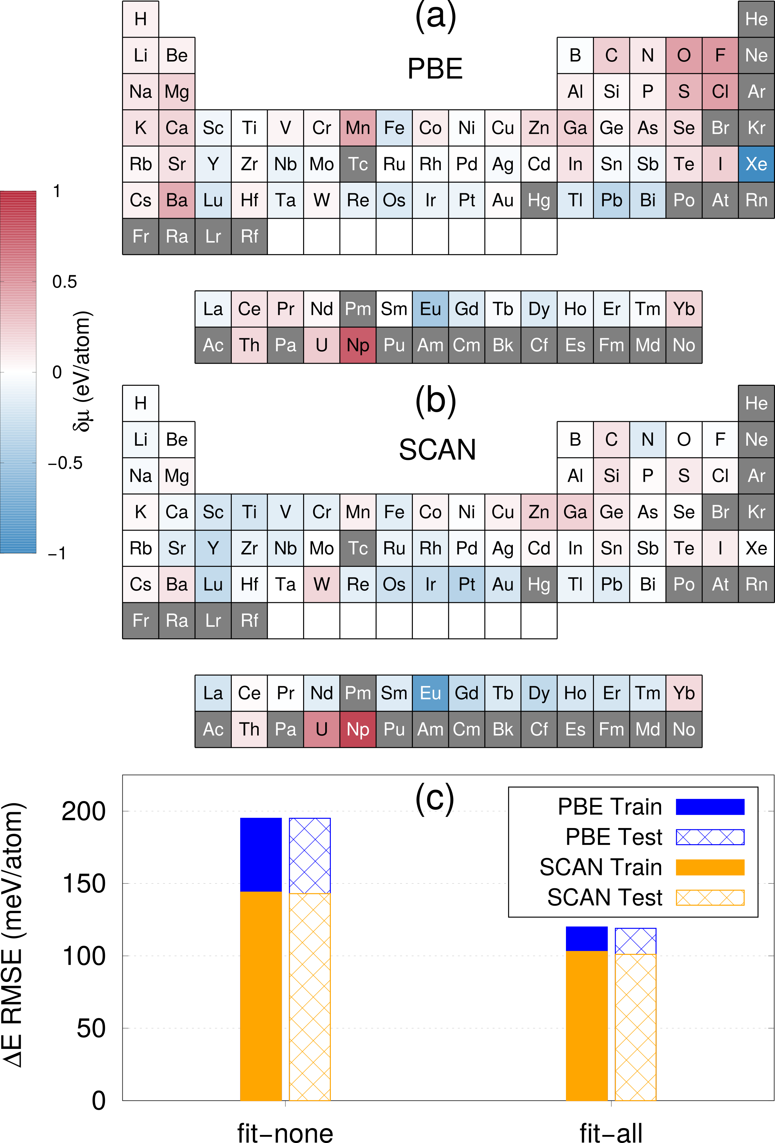
Figure 7: Elemental chemical potential corrections $\delta\mu$ obtained via fitting for (a) PBE and (b) SCAN. Grey-colored squares correspond to elements not considered in the compound set. The training and testing $\Delta E$ RMSE from 9-fold cross-validation are shown in panel (c) for the cases of fitting $\mu$ for no (“fit-none”) and all (“fit-all”) elements.

One approach to improve the quality of the predicted $\Delta H$, at the cost of adding empiricism, is to fit the elemental chemical potential $\mu$ for one or more elements Wang et al. (2006); Stevanović et al. (2012); Grindy et al. (2013); Kirklin et al. (2015). Here we perform a simultaneous least-squares fitting of $\mu$ for all 78 periodic table elements (“fit-all”) contained within our set of 945 compounds, which minimizes the RMSE of $\Delta H$. The resulting corrections to the DFT-calculated $\mu$ (which we call $\delta\mu$) are plotted in Figs. 7(a) and 7(b) for PBE and SCAN, respectively. For PBE, significant positive corrections are found for electronegative elements such as O, S, F, and Cl. These corrections are consistent with PBE’s tendency to underbind the strongly-bound compounds, which typically contain such elements. In contrast, since SCAN does not suffer from an appreciable systematic underbinding or overbinding of the strongly-bound compounds, there are no large corrections to the electronegative elements for SCAN. Since SCAN moderately overbinds intermetallic compounds, there are many more negative $\delta\mu$ for metallic elements for SCAN as compared to those of PBE. One can observe this trend for many alkali, alkaline earth, transition, and lanthanide metals.

In order to assess the possibility of overfitting, we perform 9-fold cross-validation and separately analyze the training and testing errors. Figure 7(c) illustrates the RMSE $\Delta H$ errors for PBE and SCAN for the fit-all case and that of no fitting (“fit-none”). Fitting reduces the error from 195 to 120 meV/atom for PBE and 144 to 104 meV/atom for SCAN. Since the training and testing errors are nearly identical, this indicates there is no overfitting in predicting $\Delta H$ with the set of fit $\mu$. We note that the corresponding testing MAE are 83 and 72 meV/atom for PBE and SCAN, respectively. The full set of fitted $\mu$ values are included in the Supporting Information.

IV.4 Volumes

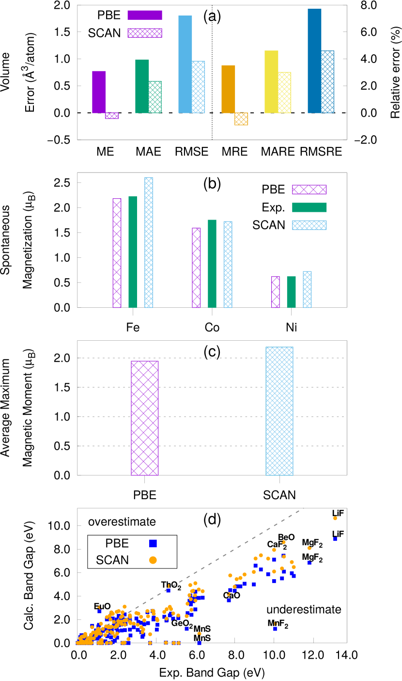
Figure 8: Comparison of predicted structural, magnetic, and electronic properties for PBE and SCAN, with experimental values shown when available. (a) Absolute and relative errors in compound volume. (b) Spontaneous magnetization for Fe, Co, and Ni. (c) Average maximum local magnetic moment for magnetic compounds. (d) Calculated and experimental electronic band gap, with the dashed line corresponding to perfect agreement.

In order to assess the accuracy of the crystal structures, we compare the computed relaxed volume per atom to experimental values taken from the ICSD. Both the compounds and solid elements are considered. Figure 8(a), which shows the absolute and relative errors for PBE and SCAN, demonstrates that SCAN achieves a significant improvement in the predicted volumes. While PBE on average overestimates the volume by 0.77 ų/atom, SCAN only underestimates it by 0.11 ų/atom. The MAE for SCAN is 0.58 ų/atom, a 41% decrease from the corresponding PBE value. The relative error magnitudes for SCAN are similarly smaller than those of PBE.

A complete plot of the predicted and experimental volumes, shown in the Supporting Information, illustrates that the SCAN’s improved prediction of volume is particularly significant for layered materials. For example, SCAN predicts a volume of 35.6 ų/atom for the layered material MgI₂ with experimental volume of 34.3 ų/atom, whereas PBE significantly overestimates the volume with a value of 40.6 ų/atom. Such improved volume prediction for layered materials is consistent with the improved treatment of (intermediate) van der Waals interaction in SCAN Sun et al. (2015). We find similar behavior for one-dimensional materials like BeI₂ and AgCN.

Unlike the behavior for $\Delta H$, the predicted volume behavior is less different between strongly- and weakly-bound compounds. The same qualitative trend, smaller errors for SCAN than PBE, is found for both sets of compounds by all error metrics considered. In addition, for SCAN the quantitative accuracy of the predicted volumes is essentially the same for the two sets of compounds. The difference in volume MAE between the two subsets of compounds is only 0.02 ų/atom for SCAN, with the slightly larger errors for strongly-bound compounds. For PBE, the difference is larger (0.50 ų/atom), also with the larger errors for strongly-bound compounds. This is consistent with the underbinding trend of $\Delta H$ for strongly-bound compounds and suggests that PBE’s treatment of the compound (as opposed to only the elements) contributes to the underbinding of $\Delta H$. Additionally, the larger errors for layered materials, which are mainly strongly-bound compounds (in the sense of large $\Delta H_{exp}$) also contribute to the worsened volume predictions for strongly-bound compounds in PBE. For example, layered ZrCl₂ with $\Delta H_{exp}$ of -1.73 eV/atom exhibits a 44% volume error within PBE (4% in SCAN). Overall, SCAN shows a significant improvement over PBE for prediction of crystal volumes with 57% and 33% MAE reductions for strongly- and weakly-bound compounds, respectively.

IV.5 Magnetism

Next, we explore the predicted magnetic properties. The spontaneous magnetization of the elemental metals Fe, Co, and Ni for PBE and SCAN as compared to experiment Crangle and Goodman (1971) are shown in Fig. 8(b). In all cases, SCAN predicts a moderately larger magnetization than that of PBE. The enhancement in magnetization is 0.42 $\mu_{B}$ (19%), 0.13 $\mu_{B}$ (8%), and 0.1 $\mu_{B}$ (14%) for Fe, Co, and Ni, respectively. For Fe and Ni, this leads to worsened comparison to experiment. For example, SCAN overestimates the magnetization of Fe by 17%, while PBE underestimates it by only 2%. In contrast, SCAN’s magnetization for Co (1.72 $\mu_{B}$) is closer to the experimental value (1.75 $\mu_{B}$) than that of PBE (1.59 $\mu_{B}$). Such results suggest a tendency of SCAN to moderately overestimate the magnetism in itinerant (ferro)magnets in some cases.

We also compare the predicted local magnetic moments of PBE and SCAN in all of the magnetic systems considered. We choose to consider a system magnetic if any local magnetic moment is greater than 0.1 $\mu_{B}$ in magnitude. Figure 8(c) shows the maximum local magnetic moment, averaged over all the magnetic systems. While the overall magnitude of this quantity (around 2 $\mu_{B}$) is not important as it is dependent on the particular set of elements and compounds studied in this work, we comment on the difference in the values between PBE and SCAN. Consistent with the behavior for the elemental ferromagnets, here SCAN again shows a moderate magnetic enhancement. In particular, the average maximum magnetic moment within SCAN is 12% larger than that found within PBE. A complete plot of the magnetic moments for all the magnetic compounds, which illustrates this trend, is included in the Supporting Information. This plot also indicates there are certain compounds predicted to be non-magnetic within PBE for which SCAN predicts magnetism (e.g., FeTe₂ and FeCl₂).

IV.6 Band gaps

Finally, we consider the performance of SCAN for electronic band gap prediction. Semilocal approximations to $E_{xc}$ like LDA and PBE are well known to underestimate band gaps Perdew (1985). Although SCAN is not specifically designed to address this band gap problem, it is interesting to evaluate its accuracy for predicting band gaps as compared to PBE, especially since SCAN in principle contains some nonlocality via $\tau$. Details of the extraction of experimental band gap values Strehlow and Cook (1973) for comparison are discussed in the Supporting Information.

Figure 8(d) compares computed band gaps to experimental values. Nearly all the points lie below the dashed line of perfect agreement, which indicates that SCAN like PBE suffers from a systematic underestimation of electronic band gap. However, the SCAN points are usually in better agreement with experiment. As one example, the SCAN band gap for GaN is 2.2 eV as compared to 3.2 eV in experiment, whereas the PBE gap is 1.7 eV. Additionally, it appears the improvement in band gap prediction for SCAN as compared to PBE becomes more significant on an absolute scale as the magnitude of the band gap increases. For example, for LiF (with a very large experimental gap of 13.1 eV), the SCAN band gap is 1.8 eV larger than that of PBE, though still underestimating the experimental value. The band gap enhancement of SCAN compared to PBE is not solely a result of structural relaxation. For example, SCAN exhibits a 0.3 eV enhancement of band gap of GaN with respect to PBE using the experimental structure, as compared to 0.5 eV using relaxed structures. For LiF, the corresponding band gap enhancement is 1.1 eV and 1.8 eV without and with structural relaxations, respectively.

Overall, we find a band gap MAE of 1.2 eV for SCAN as compared to 1.5 eV for PBE. This indicates that SCAN provides a modest improvement in band gap prediction as compared to PBE, though the band gaps still significantly underestimate experimental values. We note that fully nonlocal approaches to band gap prediction like many-body perturbation theory in the $GW$ approximation Hedin (1965); Hybertsen and Louie (1985, 1986); Faleev et al. (2004); van Schilfgaarde et al. (2006) as well as hybrid functionals like HSE Heyd et al. (2003) perform significantly better at band gap prediction Tran and Blaha (2009). For example, previous work has shown band gap MAE of 0.6 eV for HSE and 0.5 eV for $GW,$ considering the 15 compounds in Ref. 58 for which self-consistent $GW$ and HSE values are given. Another earlier work found a band gap MAE of 0.3 eV for HSE Heyd et al. (2005).

V Conclusions

In summary, an extensive benchmark of the new SCAN meta-GGA for a diverse set of approximately 1,000 inorganic crystals is performed and compared to the GGA level of theory (PBE). Unlike PBE, SCAN does not exhibit a substantial, systematic underbinding of strongly-bound compounds with respect to the elements, due to enhanced exchange interaction in the covalent bonding regime. This leads SCAN to significantly out-perform PBE for formation energies of such compounds, with a decrease in MAE of around 50% to 110 meV/atom. In contrast, due to distinct exchange behavior in the weak bonding regime, SCAN performs moderately worse than PBE for weakly-bound compounds like intermetallics, for which the formation energy MAE increases by 20% to 102 meV/atom. The formation energy errors can be further reduced by fitting the elemental chemical potentials. SCAN shows significant improvement in volume prediction, with a 41% decrease in MAE with respect to PBE to 0.58 ų/atom. A moderate magnetic enhancement is found using SCAN as compared to PBE, with a 12% increase in the average maximum magnetic moment. SCAN significantly underestimates experimental band gaps, though there are moderate improvements (20% decrease in MAE) as compared to PBE. Overall, SCAN represents a significant improvement in accuracy for strongly-bound compounds as compared to PBE.