Accounting Noise and the Pricing of CoCos

Abstract

Contingent Convertible bonds (CoCos) are debt instruments that convert into equity or are written down in times of distress. Existing pricing models assume conversion triggers based on market prices and on the assumption that markets can always observe all relevant firm information. But all Cocos issued so far have triggers based on accounting ratios and/or regulatory intervention. We incorporate that markets receive information through noisy accounting reports issued at discrete time instants, which allows us to distinguish between market and accounting values, and between automatic triggers and regulator-mandated conversions. Our second contribution is to incorporate that coupon payments are contingent too: their payment is conditional on the Maximum Distributable Amount not being exceeded. We examine the impact of CoCo design parameters, asset volatility and accounting noise on the price of a CoCo; and investigate the interaction between CoCo design features, the capital structure of the issuing bank and their implications for risk taking and investment incentives. Finally, we use our model to explain the crash in CoCo prices after Deutsche Bank’s profit warning in February 2016.
JEL codes: G12, G13, G18, G21, G28, G32
AMS subject classification: 91B25, 91G40, 97M30
Key Words: Contingent capital pricing, accounting noise, Coco triggers, Coco design, risk taking incentives, investment incentives

1 Introduction

Contingent Capital instruments or Contingent Convertible bonds (CoCos) are debt instruments designed to convert into equity or to be written down in times of distress. They differ from regular convertibles in that conversion is not an option to be exercized by the holder; conversion is either automatically triggered in response to a particular accounting ratio falling below a specified threshold or at the discretion of the regulator when a so called Point of Non-Viability (PONV) has been reached. They were originally proposed by Flannery (2005) as an alternative to raising equity in times of distress. Their use has exploded since the Great Financial Crisis eroded the capital base of banks across the world and regulators responded by actually raising capital requirements so as to increase the Loss Absorption Capacity of the banking system. In this paper we develop a valuation model that not only takes into account their particular contingent properties but also explicitly incorporates the fact that markets get only imperfect information about the underlying firm dynamics through noisy accounting reports issued at regular discretely spaced time points.

An academic literature has quickly emerged since Flannery’s original advocacy of CoCos (Flannery 2005), and unanimously recommends basing trigger ratios on market values. In line with that view, the pricing models proposed so far assume conversion triggers based on market prices. Moreover, the literature is without exception built on the assumption that markets can always observe all relevant firm information, so the existing literature in fact assumes there is no difference between accounting and market values, which makes the choice between them obviously irrelevant. Whatever the merit of that view (the preference for market based triggers), fact is that basing conversion on market prices actually makes a CoCo ineligible for being counted against capital requirements under European law (cf. Capital Requirements Regulation 575/2013/EU (2013, art. 54), henceforth referred to as CRR) under the framework implementing Basel III capital requirements in the European Union. Accordingly, all CoCos issued so far have without exception triggers for conversion based on accounting ratio’s falling below a particular ratio (the trigger ratio).

In this paper we attempt to bridge this discrepancy between the academic valuation literature on the one hand and the actual capital market practice on the other by valuing CoCos under the assumption that the only information available is noisy accounting information, our first contribution, which in addition is only received at pre-specified discrete moments in time. The underlying processes are continuous, but markets only receive noisy information on those underlying fundamental processes at discrete time instants: accounting reports are only released at discretely spaced points in time, the accounting dates (for example at the end of each quarter). In this way it is possible to distinguish between market and accounting values. This informational structure gives rise to potential discrepancies between true underlying values, accounting ratios and market prices.

We make a second contribution towards a better pricing model for CoCos. The asset pricing literature has so far concentrated on the conversion contingency. But the possibility of a write down or conversion into equity is not the only option-like characteristic embedded in CoCo designs. The coupon payments are contingent too, they can only be paid out if that payment does not exceed the so called Maximum Distributable Amount, a trigger that binds much earlier than the conversion trigger (see (Kiewiet et al. 2017) for extensive details). The relevance of this contingency became very clear in the beginning of 2016, when a profit warning of Deutsche Bank ahead of their first quarter accounting report set off an accross the board crash in CoCo prices (cf. again Kiewiet et al. (2017)).

The model developed in this paper thus contributes in two different ways to the existing literature; it distinguishes between market and book values of assets in the valuation of CoCos and it allows the coupons of CoCos to be already cancelled at a moment before the conversion date. The model is based on the approach used by Duffie and Lando (2001), in which debt is valued under the assumption that the only information available is noisy accounting information which is received at selected moments in time. This setting is particularly relevant for the pricing of CoCos since, as pointed out above, the non-discretionary conversion triggers are always based on imperfect accounting ratios observed at discrete moments in time, rather than on continuously observable market prices.

We first set up a comprehensive description of the structural credit risk model proposed by Duffie and Lando, including the derivation of all the relevant formulas and proofs. We then go beyond the paper by Duffie and Lando by using their framework to provide explicit formulas and algorithms for the pricing of CoCos. The setting is applied to the valuation of different kinds of CoCo bonds, namely CoCos with a (partial) principal write down and CoCos with a conversion into shares. Also a distinction is made between CoCos with a discretionary regulatory trigger, for which conversion could happen at any moment in time, and CoCos that can only be triggered at one of the accounting dates. The model does not lead to closed form solutions, but the expressions for CoCo prices involve integrals that are computed using MCMC-methods.

We first use the model developed in this paper to examine the impact of several CoCo design parameters on the price of a CoCo; we then investigate the interaction between CoCo design features, the capital structure of the issuing bank and their implications for risk taking and investment incentives. Finally, the model is used to explain the big downward price jump that CoCos of Deutsche Bank suffered at the beginning of 2016 after the release of a profit warning. In this particular case the added value of the proposed model becomes clear as it allows for the announcement of a bad accounting report and explicitly allows for the early cancellation of coupon payments (before conversion) when the payment would exceed the so called Maximum Distributable Amount (MDA) trigger, cf. Pitt and Dewji (2016). Market sources indeed indicated at the time that the sudden price drop was out of fear for the MDA trigger more than for setting off the conversion trigger, as the conversion trigger was still far out of reach.

The remainder of this paper is as follows. Section 2 describes CoCos in detail, their design features and their regulatory treatment. Section 3 surveys the existing asset price literature on CoCos. Section 4 sets up the pricing model, making a distinction between market values and accounting values and incorporating the possibility of early cancelling of coupons triggered by the MDA regulations referred to earlier, Section 5 outlines the MCMC algorithms used for evaluating the integrals involved in the final pricing expressions. We outline the derivation of the key pricing formulas, with full details in the Appendix. Section 6 uses the model to analyse the sensitivity of CoCo valuation to various design features, changes in the firm’s capital structure and various external shocks. We also analyse the events following Deutsche Bank’s profit warning of late February 2016, and show that our pricing model does quite well in explaining the observed CoCo price response. Section 7 summarizes and concludes. Proofs of the technical results are collected in the Appendix.

2 Contingent convertible bonds

A Contingent Convertible bond is a bond which converts into equity or is (partially) written down at the conversion date. This means that the design of a CoCo contract is specified by two main characteristics:

• The trigger event: when does conversion happen?

• The conversion mechanism: what does happen at conversion?

2.1 The trigger event

The trigger event specifies at which moment the conversion takes place. We can distinguish three types of trigger events; an accounting trigger, a market trigger and a regulatory trigger. In case of an accounting trigger, the conversion is triggered by an accounting ratio, e.g. the Common Equity Tier 1 Ratio (defined as the fraction of common equity over (risk weighted) assets) falling below a certain barrier. This type of trigger is typical in practice, although it is widely criticized in the academic world. For example, in Flannery (2005) it is argued that a book value will only be triggered long after the damage has already occurred, because book values are not up-to-date at any moment. Therefore, the academic literature widely supports the use of market price based triggers. In the case of a market trigger, the conversion happens if a market value, e.g. the share price of the issuing bank, falls below a certain threshold. A market price is thought to better reflect the current situation of the issuing bank, because a market price is a forward looking parameter; it reflects the market’s opinion on the future of the bank. See Haldane (2011) and also Pennacchi and Tschistyi (2015) for a very articulate defense of this point of view, to which we return in the next section. Against this point of view, in Sundaresan and Wang (2015) and Glasserman and Nouri (2016) it is argued that a market trigger could lead to a multiple equilibria problem for the pricing of a CoCo if the terms of conversion are beneficial to CoCo holders. In this case, a market trigger could also encourage CoCo holders to short-sell shares of the issuing bank, to profit from a conversion, which could subsequently lead to a “death spiral”. These warnings may well explain why market based triggers are actually outlawed in the European Union, cf. CRR. Whatever the EU’s reason for this outlawing of market based triggers, as a consequence no CoCos with market price based triggers have been issued so far. A third type of trigger is the regulatory trigger, which allows the regulator to call for a conversion. All CoCos issued so far have a trigger mechanism which is a combination of an accounting trigger and a regulatory trigger, since that is required for the CoCo to count as regulatory capital in the European Union. The regulatory trigger has not been discussed in the asset pricing literature yet (but see Chan and van Wijnbergen (2018) for a corporate finance perspective on CoCo triggers focusing on risk taking and regulatory forbearance, i.e. regulatory behavior).

2.2 The Conversion mechanism

The conversion mechanism specifies what happens at the moment of conversion. There are two possibilities: a (partial) principal write-down or a conversion into shares. In case of a (partial) principal write-down (PWD) mechanism, the principal of the CoCo bond is (partially) written down at the moment of conversion, to strengthen the capital position of the issuing bank. In case of a conversion into shares, the principal of the CoCo bond is converted into a number of shares. Of course, it needs to be specified how many shares a CoCo holder receives at conversion. This conversion rule can be designed in two different ways. One possibility is that the CoCo holder receives a fixed number of shares $\Delta$ for every monetary unit of principal. This corresponds to a pre-specified share price $1/\Delta$. Another option is a variable number of shares related to the market price prevailing at the moment of time conversion takes place. In this case the CoCo holder would “buy” a number of shares against a market price based conversion price. Some authors have warned for the possibility of a “death spiral” when CoCo conversion is advantageous to CoCo holders and thus leads to incentives to short sell the stock (cf. Sundaresan and Wang (2015)). This possibly leads to an infinitely large dilution of the existing shareholders. A way to avoid this would be to place a floor under the conversion price, again a requirement for the CoCo to count as capital under European law.

2.3 The Maximum Distributable Amount (MDA) trigger

As Contingent Convertible bonds qualify as a form of capital in the Basel III regulations, they are also affected by the concept of the Maximum Distributable Amount (MDA), which requires regulators to block earnings distributions when the bank’s capital becomes too low. An example of such earnings distributions are dividends, but also CoCo coupon payments if the CoCos qualify as AT1 capital. This means that when the bank’s capital falls below some threshold, always (much) higher than the CoCo’s conversion trigger, the payment of coupons is stopped until the bank’s capital is again above the MDA trigger. See Kiewiet et al. (2017) for a detailed discussion of the MDA trigger for coupons. This trigger has not been considered before in the asset pricing literature, but will be introduced explicitly in this paper.

3 Related Literature

The existing asset pricing literature on CoCos can be grouped in three categories (cf. Wilkens and Bethkens (2014) for an early assessment following the same classification): structural models, equity derivative models and credit risk or reduced form models. In a structural model one starts by describing the value of the assets of a firm by a stochastic process. Then the liabilities are introduced and equity is the difference between the assets and those liabilities. Conversion of CoCos occurs when the market value of the firm’s assets or the firm’s capital ratio falls below a predetermined value (the conversion trigger). In most papers, liquidation of the firm is also incorporated in the model by assuming that the equity holders liquidate the firm when the value of assets falls below some optimal threshold, chosen by the shareholders to maximize equity value. Furthermore, it is assumed that default cannot occur before conversion. An early example of such a structural model is Albul et al. (2012); there the firm’s value $A_{t}$ is described by a geometric Brownian motion (GBM) process under the Risk Neutral measure given by

$$\mathrm{d}A_{t} = \mu A_{t}\,\mathrm{d}t+\sigma A_{t}\,\mathrm{d}W_{t},$$

with $\mu$ and $\sigma$ constants and $W$ a standard Brownian motion. The risk-free rate is assumed constant. The firm also issues two types of debt: a straight bond and a CoCo, both with perpetual maturities and both paying coupons at a constant rate. The CoCo converts into equity the first time the asset value falls below some threshold $\alpha_{c}$, so the conversion time is $\tau(\alpha_{c})=\inf\{t\geq 0:A_{t}\leq\alpha_{c}\}$. In their set up, the CoCo converts into equity valued at market prices at a specified conversion ratio $\lambda$, where $\lambda=1$ means that the CoCo holder receives equity with a market value equal to the face value of the CoCo at issue. Like in all other papers surveyed here, the value of the various claims (including the CoCos) is given by the risk-neutral expectation of the discounted future cashflows regarding the claim. The simplicity of the model allows for closed form expressions. In Pennacchi (2011) a similar model is introduced, but also proportional jump processes are added to the firm’s dynamics by adding a compound Poisson process; asset values are governed by the following stochastic process (also under the risk neutral measure)

$$\mathrm{d}A_{t} = (r-\lambda_{t}k_{t})A_{t}\,\mathrm{d}t+\sigma A_{t}\,\mathrm{d}W_{t}+(Y_{q_{t}}-1)\,\mathrm{d}q_{t}.$$

Here $\lambda_{t}$ is the risk neutral jump intensity of the Poisson process $q_{t}$, $k_{t}=E_{Q}(Y-1)$ is the expected proportional jump under the risk neutral measure in case a Poisson jump occurs. The model does not yield closed form solutions so Monte Carlo simulation is used to sketch the solution structure. In Chen et al. (2013) an equally involved model is proposed in which the asset value process also involves a GBM process with Poisson jumps added in, with a distinction between market wide and firm specific jumps. They are mainly interested in downside shocks and, for tractability, they assume that minus the log of the jump sizes have exponential distributions, which allows the authors to derive closed form solutions. Conversion of CoCos into equity is triggered the first time the value of assets falls below some specified threshold. In contrast to the variable conversion share price featured in Albul et al. (2012) and Pennacchi (2011), the CoCo holders receive a fixed number of shares for every dollar of principal when the CoCo converts, which is the way all Cocos with a conversion into shares are set up in practice, cf. Avdiev et al. (2017). An interesting innovation is their introduction of finite maturity debt and the associated potential debt roll over problems. This feature has a significant effect on risk taking behavior before conversion: even when the share conversion takes place at a rate favorable to the old shareholders, conversion leads to higher roll over costs of short term debt, which mitigates risk taking incentives ex ante. The model in Pennacchi and Tschistyi (2015) reverts to a straight GBM process driving asset values, and the focus is on the uniqueness and in fact existence of a price equilibrium when conversion involves a wealth transfer favoring either the CoCo holder (dilutive CoCos) or the old equity holder (non-dilutive CoCos). Academics widely favor conversion triggers based on market prices and dilutive conversion ratios, but in Sundaresan and Wang (2015) it has been argued that stipulating triggers based on market prices leads to multiple price equilibria in the case of dilutive CoCos and in fact non-existence in the case of non-dilutive CoCos (i.e. conversion at terms favoring the old shareholders). Both in Glasserman and Nouri (2016) and Pennacchi and Tschistyi (2015) it is shown that price equilibria will in fact be unique in the case of dilutive CoCos. In Pennacchi and Tschistyi (2015) it is furthermore shown that for perpetual CoCos (which is the structure most seen in practice) non-existence only occurs for implausible parameter values even when they are non-dilutive.

All these models have in common that a conversion trigger based on market values is used, as is widely recommended in the academic literature (cf. in particular Haldane (2011) and Pennacchi and Tschistyi (2015) for an extensive discussion of why market prices should be used for conversion triggers). The problem with basing one’s analysis on that view, whatever its merit, is that there is literally no single CoCo ever issued, at least within the European Union, that follows such a trigger definition. Without exception, within the European Union, where the bulk of all CoCos have been issued, trigger ratios are based on accounting values. In fact in the EU, market based triggers are illegal under European law, cf. CRR, or at least cannot be counted as capital.

Moreover, none of the models discussed so far actually distinguishes between market and accounting based valuation. The single exception in the literature is Glasserman and Nouri (2012), where it is assumed that markets and accountants agree on whether a firm is solvent (if the value of the assets exceeds the value of debt based on market prices, accounting values are assumed to do likewise). But the ratio between the market value of equity and the accounting value of equity, roughly similar to the market-to-book (M-to-B) ratio, follows a GBM process. This approach gives two additional parameters to be used in calibration: the volatility of the M-to-B value process and its correlation to the market process. This is an imaginative attempt to endogenize the M-to-B value process, but there are problems with this first attempt at endogenizing the difference between market values and accounting ratios. First of all, Haldane (2011) doubted casts on their key assumption, that market and accounting valuations always agree on whether the firm is solvent. A less fundamental but practically speaking equally serious problem is that the approach in Glasserman and Nouri (2012) assumes that all processes can be observed continuously. In practice however regulatory capital ratios are only calculated on a quarterly basis.

In this paper we address both shortcomings. We assume that firm values are driven by a GBM, without jumps; we omit jumps for reasons explained in Section 4. We do not introduce a separate independent accounting process like Brigo et al. (2015). Instead we follow the approach taken in Duffie and Lando (2001) who assume an underlying GBM process for the dynamic evolvement of the firm’s asset valuation, but stipulate that that process is not directly observable. Instead, noisy information (“accounting report”) is brought out at discrete time instants (“quarters”). It is reasonable that noise in accounting reports has some persistence, so we assume that the noise term in the accounting report is serially correlated. See Section 4 again for a detailed description.

In addition to these structural models, the literature has seen two other approaches, the credit derivative approach and an equity derivative approach. A credit derivative approach is a reduced form approach where a conversion arrival intensity exists by assumption and is subsequently modeled as a function of latent state variables or predictors of future conversions. This approach is appealing for its tractability but is difficult to apply empirically for the simple reason that conversions have not yet occurred in practice, making the latent variable approach untestable in practice as of the date of writing this article. However it could be useful in linking observed credit spreads on CoCos to presumed drivers of conversion arrival intensities. A third approach, described in Wilkens and Bethkens (2014), is the equity derivative approach where one tries to replicate the CoCo pay off by using equity derivatives directly. The CoCo is seen as a straight bond plus Knock-in Forwards minus Binary Down-in options. The long position in Knock-in Forwards correspond to the possible purchase of shares at the stipulated conversion price in case the trigger event takes place (i.e. when the forwards knock in). The short position in Binary Down-in options reflects the loss of (parts of) the coupon payments once the trigger event occurs. A shortcoming of this approach is that it assumes the investor receives forwards at conversion; but in an equity converter CoCo the investor receives shares, not forwards. This is a significant difference when the trigger event happens a substantial time before expiration of the CoCo. This matters since CoCos must be perpetuals to qualify as capital. If dividends are expected to be low for a substantial period of time after the trigger event occurs, this may not be a major shortcoming. A bigger problem with both the credit derivative and the equity derivative approach is that they unavoidably have to assume trigger events conditional on market price based triggers, which is counterfactual. A third problem with the two derivative based approaches is that if they are to remain analytically tractable, one has to assume a Black-Scholes setting for the market price which cannot easily handle the fat tail risk observed in CoCo prices and cannot incorporate the link between fat tail risk and accounting reports observed in practice, cf. Kiewiet et al. (2017). In Corcuera et al. (2013) it is shown that this problem can be addressed by analyzing an equity derivative based model using ”smile conform” exponential Lévy processes for stock price dynamics, incorporating jumps and fat tails, but this approach unavoidably comes at the cost of having to replace analytical closed form solutions by simulation based solutions.

4 The Model

This section starts with the model description. After that we derive the density of asset values, conditional on accounting information. Finally we present results for the valuation of CoCos for the different trigger events: regulatory triggers, possibly with conversion into shares, and accounting triggers.

4.1 Model Description and the Firm’s Debt Structure

The value of assets of the firm, denoted by $V_{t}$, is modeled by a geometric Brownian motion, that is

$$\frac{\mathrm{d}V_{t}}{V_{t}}=\mu\mathrm{d}t+\sigma\mathrm{d}W_{t},$$ (4.1)

for some $\mu\in\mathbb{R}$, $\sigma>0$. We will not explicitly include jumps in the asset value process, because this does not make sense in the noisy accounting information framework, as it would not be possible to distinguish a big price movement caused by the dynamics of the asset process from a reaction to the accounting information. Define $Z_{t}=\log V_{t}$ and $m=\mu-\sigma^{2}/2$, then $Z$ is a drifted Brownian motion with drift $m$ and volatility $\sigma$, that is

$$Z_{t}=Z_{0}+mt+\sigma W_{t}.$$

As mentioned before, we will consider a framework in which investors do not observe the real asset value, instead they receive imperfect accounting information at known observation times $t_{1}<t_{2}<\dots$ (typically every three months). At every observation date $t_{i}$ there arrives an imperfect accounting report of the real asset value $V_{t_{i}}$, denoted by $\hat{V}_{t_{i}}$, where $\log\hat{V}_{t_{i}}$ and $\log V_{t_{i}}$ are assumed to be joint normal. This means that we can write

$$Y_{t_{i}}:=\log\hat{V}_{t_{i}}=Z_{t_{i}}+U_{t_{i}},$$ (4.2)

where $U_{t_{i}}$ is normally distributed and independent of $Z_{t_{i}}$. In the following we will use the notation $Y_{i}:=Y_{t_{i}}$ and similar notations for $Z$ and $U$. Of course, it is reasonable that there exists some correlation between the accounting noise $U_{1},U_{2},\dots$. To be more specific, following Duffie and Lando (2001), it is assumed that

$$U_{i}=\kappa U_{i-1}+\epsilon_{i},$$

for some fixed $\kappa\in\mathbb{R}$ and independent and indentically distributed $\epsilon_{1},\epsilon_{2},\dots$, which have a normal distribution with mean $\mu_{\epsilon}\in\mathbb{R}$ and variance $\sigma_{\epsilon}^{2}>0$, and are independent of $Z$.
It is assumed that the firm issues two types of debt; straight debt and contingent convertible debt. The total par value of straight debt outstanding is denoted by $P_{1}$, over which coupons are paid continuously at rate $c_{1}$. Furthermore, the straight bonds have a perpetual maturity and it is assumed that default occurs the first time the $\log$-value of assets falls below some threshold $z_{b}$, such that the default time is defined by

$$\tau_{b}=\inf\{t\geq 0:Z_{t}\leq z_{b}\}.$$

At the moment of default a fraction $(1-\alpha)$, for $\alpha\in(0,1)$, of the firm’s asset value is lost to bankruptcy costs, so a fraction $\alpha$ of the asset value is recovered and distributed among the senior debt holders.
The total par value of CoCos outstanding is denoted by $P_{2}$, over which coupons are paid continuously at rate $c_{2}$. Furthermore, the maturity of the contingent convertible bonds is denoted by $T$. In our accounting report framework, we will consider two different types of conversion triggers. The first type of conversion trigger that will be looked into is the regulatory trigger. Banks have the obligation to report it to their supervisor at the moment they are approaching a trigger. Then the regulator will call for conversion, this is called a Point of Non-Viability. Of course, this type of conversion can also happen in between accounting report dates. This type of conversion thus is triggered when the $\log$-value of assets falls for the first time below a conversion threshold $z_{c}$, i.e. the conversion time is given by

$$\tau_{c}=\inf\{t\geq 0:Z_{t}\leq z_{c}\}.$$

We will always assume that $z_{b}<z_{c}$, such that conversion will always happen before default, i.e. $\tau_{c}<\tau_{b}$.
There are also also CoCos whose conversion trigger solely depends on accounting reports. An example is the Coco issued by Barclays on March 3, 2017 (cf. Barclays (2017)). This means that conversion happens when the reported value of the capital ratio falls below some threshold and hence conversion can only happen at one of the accounting report dates $t_{1},t_{2},\dots$. This corresponds to a setting in which the conversion time is defined as

$$\tau_{c}^{A}=\inf\{t_{i}\geq 0:Y_{t_{i}}\leq y_{c}\},$$

for some threshold $y_{c}\geq 0$.
In case we consider CoCos with regulatory triggers, the information available to investors at time $t$ is described by the filtration $\mathcal{H}_{t}$, where

$$\mathcal{H}_{t}=\sigma(\{Y_{t_{1}},\dots Y_{t_{n}},\mathbf{1}_{\{\tau_{c}\leq s\}},\mathbf{1}_{\{\tau_{b}\leq s\}}:s\leq t\}),\text{ for }t_{n}\leq t<t_{n+1}.$$

Here, the indicators are included to ensure that it is also observed in the market whether conversion has already occured or the firm is liquidated before time $t$. In case we deal with CoCos with an accounting trigger, the market information is described by the filtration

$$\mathcal{H}_{t}=\sigma(Y_{t_{1}},\dots Y_{t_{n}}),\text{ for }t_{n}\leq t<t_{n+1}.$$

4.2 The Density of Asset Value, Conditional on Accounting Information

In the previous subsection it was explained that we will consider two different types of conversion triggers. For the first one, the regulatory trigger, the conversion time is determined by the process $Z$ falling below some threshold. In order to compute the market value of CoCos with such a trigger, we need to be able to compute the probability of conversion, conditional on the market information $\mathcal{H}_{t}$. In order to do so, we will need the conditional density of $Z$, given the market information $\mathcal{H}_{t}$. In this subsection, following Duffie and Lando (2001), we will derive an expression for this conditional density, which is intensively used in the remainder of this article.
Consider $t>0$ such that $t_{n}\leq t<t_{n+1}$ and conversion did not happen until time $t$, that is $\tau_{c}>t$. The goal in this section is to find an expression for the conditional distribution of $Z_{t}$, given $\mathcal{H}_{t}$, which we will denote by $f(t,\cdot)$. Most of the results in this section can be found in the article by Duffie and Lando (2001), but we will consider them shortly, to illustrate how the particular density is derived and we will provide some additional explicit formulas.
Consider the following notation for the relevant random vectors and its realisations:

$$Z^{(n)}=(Z_{1},Z_{2},\dots,Z_{n})\text{ and its realisation }z^{(n)}=(z_{1},z_{2},\dots,z_{n}),$$

$$Y^{(n)}=(Y_{1},Y_{2},\dots,Y_{n})\text{ and its realisation }y^{(n)}=(y_{1},y_{2},\dots,y_{n}),$$

$$U^{(n)}=Y^{(n)}-Z^{(n)}\text{ and its realisation }u^{(n)}=y^{(n)}-z^{(n)}.$$

As already mentioned, the goal is to compute $f(t,\cdot)$, the conditional density of $Z_{t}$ given $Y^{(n)}$ and $\tau_{c}>t$. In order to do so, we will first compute the conditional density of $Z_{t_{n}}$ at the report time $t_{n}$, which we will denote by $g_{t_{n}}(\cdot|Y^{(n)},\tau_{c}>t_{n})$. To this end, we will first introduce some functions. Firstly, we need an expression for the probability $\psi(z_{0},x,\sigma\sqrt{t})$ that $\min\{Z_{s}:s\leq t\}>0$, conditional on $Z_{0}=z_{0}>0$ and $Z_{t}=x>0$. This expression is stated in the following lemma and can also be found in the paper by Duffie and Lando (2001).

• The probability $\psi(z_{0},x,\sigma\sqrt{t})$ that $\min\{Z_{s}:s\leq t\}>0$, conditional on $Z_{0}=z_{0}>0$ and $Z_{t}=x>0$, is given by

  $$\psi(z_{0},x,\sigma\sqrt{t})=1-\exp\left(-\frac{2z_{0}x}{\sigma^{2}t}\right).$$

Consider the conditional probability of the intersection $\{Z^{(n)}\leq z^{(n)}\}\cap\{\tau_{c}>t_{n}\}$ given $Y^{(n)}$. We denote by $b_{n}(\cdot|Y^{(n)})$ its partial derivative w.r.t. $z^{(n)}$. Note that $(Z_{n})_{n\in\mathbb{N}}$ and $(U_{n})_{n\in\mathbb{N}}$ are Markov processes and denote by $p_{Z}(z_{n}|z_{n-1})$ and $p_{U}(u_{n}|u_{n-1})$ their respective transition densities for realisations $z^{(n)},u^{(n)}$. Furthermore, denote by $p_{Y}(y_{n}|y^{(n-1)})$ the conditional density of $Y_{n}$ given $Y^{(n-1)}=y^{(n-1)}$. It is then possible (see Duffie and Lando (2001)) to write $b_{n}(z^{(n)}|y^{(n)})$ in a recursive way,

$$b_{n}(z^{(n)}|Y^{(n)})=$$

$$\frac{\psi(z_{n-1}-z_{c},z_{n}-z_{c},\sigma\sqrt{t_{n}-t_{n-1}})p_{Z}(z_{n}|z_{n-1})p_{U}(y_{n}-z_{n}|y_{n-1}-z_{n-1})b_{n-1}(z^{(n-1)}|y^{(n-1)})}{p_{Y}(y_{n}|y^{(n-1)})}.$$ (4.3)

It now follows that the conditional density $g_{t_{n}}(\cdot|Y^{(n)},\tau_{c}>t_{n})$ of $Z^{(n)}$ is given by

$$g_{t_{n}}(z^{(n)}|y^{(n)},\tau_{c}>t_{n})=\frac{b_{n}(z^{(n)}|y^{(n)})}{\int_{(z_{c},\infty)^{n}}b_{n}(z^{(n)}|y^{(n)})\mathrm{d}z^{(n)}}.$$ (4.4)

It should be noted that there is no explicit expression for the integral in the denominator of Equation (4.4), but note the important fact that we know the density up to a normalizing constant. Now the marginal conditional density of $Z_{n}$ at time $t_{n}$ is given by

$$g_{t_{n}}(z_{n}|y^{(n)},\tau_{c}>t_{n})=\int_{(z_{c},\infty)^{n-1}}g_{t_{n}}(z^{(n)}|y^{(n)},\tau_{c}>t_{n})\mathrm{d}z^{(n-1)}.$$ (4.5)

Now that we found the conditional density for a report time $t_{n}$, we can use this to find the conditional density $f(t,\cdot)$ for a general time $t>0$. For this we will need the $\mathcal{H}_{t}$-conditional density of $Z_{t}$, at a time before the first accounting report has arrived. Complementing Duffie and Lando (2001), we will now give an explicit expression for this density.

• $\tilde{f}(t,\cdot,z_{0})$, the $\mathcal{H}_{t}$-conditional density of $Z_{t}$, at a time $t<\tau_{c}$ before the first accounting report has arrived, given that $Z$ started in $z_{0}$, is given by

  $$\tilde{f}(t,x,z_{0})=\frac{1}{\sigma\sqrt{t}}\frac{\exp\left(\frac{-m(z_{0}-x)}{\sigma^{2}}-\frac{m^{2}t}{2\sigma^{2}}\right)\left(\phi\left(\frac{z_{0}-x}{\sigma\sqrt{t}}\right)-\phi\left(\frac{-z_{0}-x+2z_{c}}{\sigma\sqrt{t}}\right)\right)}{\Phi\left(\frac{z_{0}-z_{c}+mt}{\sigma\sqrt{t}}\right)-e^{-2m(z_{0}-z_{c})/\sigma^{2}}\Phi\left(\frac{z_{c}-z_{0}+mt}{\sigma\sqrt{t}}\right)}.$$ (4.6)

Proof.

The proof of this lemma can be found in the Appendix. ∎

Finally, we are now able time to compute the conditional density $f(t,\cdot)$ for a general time $t>0$, $t_{n}<t<t_{n+1}$ such that $\tau_{c}>t$. Using the stationarity of $Z$, the $\mathcal{H}_{t}$-conditional density of $Z_{t}$ can be written as

$$f(t,x)=\int_{z_{c}}^{\infty}\tilde{f}(t-t_{n},x,z_{n})g_{t_{n}}(z_{n}|Y^{(n)},\tau_{c}>t_{n})\mathrm{d}z_{n}.$$ (4.7)

Equation (4.7) should be read as follows; until time $t_{n}$ the process $Z$ has stayed above $z_{c}$ and ended in $z_{n}$, then on the time interval $(t_{n},t)$, in which no new accounting reports arrive, the process has to move from $z_{n}$ to $x$ and stay above $z_{c}$. Although we do not have an analytical expression for the density $f(t,\cdot)$, it is important to note at this point that $f(t,\cdot)$ is written as the integral of $g_{t_{n}}$, which is known up to normalizing constant, as can be seen from Equation (4.4). This makes it possible to compute integrals with respect to $f(t,\cdot)$, using Monte Carlo Markov Chain simulations, which means that results that are stated as an integral weighted by the density $f(t,\cdot)$ can actually be computed. The necessary algorithms are described in Section 5.
As a first use of the density $f(t,\cdot)$, we can for a time $s>t$, where $t<\tau_{c}$, define the $\mathcal{H}_{t}$-(CoCo) survival probability $p_{c}(t,s)=\mathbb{P}(\tau_{c}>s|\mathcal{H}_{t})$. This probability is then given by

$$p_{c}(t,s)=\int_{z_{c}}^{\infty}(1-\pi(s-t,x-z_{c}))f(t,x)\mathrm{d}x,$$ (4.8)

where, as in Duffie and Lando (2001), $\pi(t,x)$ denotes the probability that $Z$ hits $0$ before time $t$, starting from $x>0$. This probability is given by the following lemma, which follows from the well known expression for the distribution of a Brownian motion’s running minimum (see e.g. Harrison (1985), Section 1.8, equation (11)).

• The probability $\pi(t,x)$ that $Z$ hits $0$ before time $t$, starting from $x>0$, is given by

  $$\pi(t,x)=1-\Phi\left(\frac{x+mt}{\sigma\sqrt{t}}\right)+e^{-2mx/\sigma^{2}}\Phi\left(\frac{-x+mt}{\sigma\sqrt{t}}\right).$$

4.3 Valuation of CoCos

In this subsection we will provide formulas for the market values of the different type of CoCos. Firstly, in subsection 4.3.1, CoCos with a regulatory trigger which suffer a principal write down at conversion, are valued. Then, it is also shown how to incorporate early cancelling of coupons, due to the MDA-regulations. In subsection 4.3.2, we then extend the PWD-assumption to CoCos with a conversion into shares. These first two cases are all for the regulatory trigger and the results are all in the form of an integral weighted by the the above derived conditional density $f(t,\cdot)$. It is postponed to Section 5 to provide the necessary Algorithms to compute this integrals. Then, in Section 4.3.3, PWD CoCos with only an accounting trigger are valued.

4.3.1 Valuation of PWD CoCos with a regulatory trigger

In this section we will value CoCos with a regulatory trigger and a principal write down at conversion. At the end of the section we will also incorporate the MDA-trigger. Recall that in case of a regulatory trigger, the conversion date was defined as

$$\tau_{c}=\inf\{t\geq 0:Z_{t}\leq z_{c}\}.$$

Also, recall that the firm pays coupons continuously at rate $c_{2}$ until either maturity or conversion. We consider a principal write down CoCo, which means a fraction $1-R$ of the principal value is written down at conversion, while a fraction $R$ is recovered to the bond holder, for $R\in[0,1)$. Furthermore it is assumed that the risk free rate is constant, denoted by $r$.
Now the value at time $t<\tau_{c}$ of the CoCos, given the imperfect accounting information $\mathcal{H}_{t}$, is given by

$$C(t) =\mathbb{E}\left(P_{2}e^{-r(T-t)}\mathbf{1}_{\{\tau_{c}>T\}}|\mathcal{H}_{t}\right)+\mathbb{E}\left(\int_{t}^{T}c_{2}P_{2}e^{-r(u-t)}\mathbf{1}_{\{\tau_{c}>u\}}\mathrm{d}u|\mathcal{H}_{t}\right)$$

$$\quad+\mathbb{E}\left(RP_{2}e^{-r(\tau_{c}-t)}\mathbf{1}_{\{\tau_{c}\leq T\}}|\mathcal{H}_{t}\right)$$

$$=P_{2}e^{-r(T-t)}p_{c}(t,T)+c_{2}P_{2}\int_{t}^{T}e^{-r(u-t)}p_{c}(t,u)\mathrm{d}u-RP_{2}\int_{t}^{T}e^{-r(u-t)}p_{c}(t,\mathrm{d}u).$$ (4.9)

Here the first term represents the payment of the principal, in case conversion does not happen before maturity, while the second term accounts for the payment of coupons until either conversion or maturity. The last term values the recovery of the principal at conversion. Note that every term is written in terms of the CoCo survival probability $p_{c}(t,s)$, which was given as an integral, weighted by the density $f(t,\cdot)$. Unsurprisingly, it turns out that these three terms together can be written as one integral weighted by the conditional density $f(t,\cdot)$, which was derived in the previous section. This leads to the main result of this subsection, which is proved in the Appendix.

• The secondary market price of the CoCo at time $t<\tau_{c}$ is given by

  $$C(t)=\int_{z_{c}}^{\infty}h(x)f(t,x)\mathrm{d}x,$$ (4.10)

  where $h(x)$ is defined as

  $$h(x):=\frac{r-c}{r}P_{2}e^{-r(T-t)}(1-\pi(T-t,x-z_{c}))+\frac{c_{2}}{r}P_{2}+\left(\frac{c_{2}P_{2}}{r}-RP_{2}\right)I(x),$$ (4.11)

  in which $I(x)$ is given by

  $$I(x) :=\exp\left(-\frac{m(x-z_{c})+(x-z_{c})\sqrt{m^{2}+2r\sigma^{2}}}{\sigma^{2}}\right)\left(\Phi\left(\frac{x-z_{c}-\sqrt{m^{2}+2r\sigma^{2}}(T-t)}{\sigma\sqrt{T-t}}\right)-1\right)$$

  $$\leavevmode\nobreak\ \leavevmode\nobreak\ \leavevmode\nobreak\ +\exp\left(-\frac{m(x-z_{c})-(x-z_{c})\sqrt{m^{2}+2r\sigma^{2}}}{\sigma^{2}}\right)\left(\Phi\left(\frac{x-z_{c}+\sqrt{m^{2}+2r\sigma^{2}}(T-t)}{\sigma\sqrt{T-t}}\right)-1\right),$$ (4.12)

  where $\Phi$ denotes the normal cumulative distribution function.

In the valuation of the firm’s convertible debt in Equation (4.3.1), it is assumed that coupons are paid until conversion. However, as pointed out before, CoCos are affected by the Maximum Distributable Amount (MDA), which requires regulators to stop earnings distributions when the firm’s total capital falls below some trigger, higher than the conversion trigger. This we will incorporate in the model by introducing a trigger $z_{cc}>z_{c}$. If $Z$ is below $z_{cc}$ the firm will not pay coupons, while if $Z$ is above $z_{cc}$ the firm still pays coupons. To value the CoCo in this case, only the second term in Equation (4.3.1) needs to be adjusted. In this case, coupons are only paid at time $u$ if $Z_{u}>z_{cc}$, so the term

$$\mathbb{E}\left(\int_{t}^{T}c_{2}P_{2}e^{-r(u-t)}\mathbf{1}_{\{\tau_{c}>u\}}\mathrm{d}u|\mathcal{H}_{t}\right),$$

needs to be replaced with

$$\mathbb{E}\left(\int_{t}^{T}c_{2}P_{2}e^{-r(u-t)}\mathbf{1}_{\{\tau_{c}>u,Z_{u}>z_{cc}\}}\mathrm{d}u|\mathcal{H}_{t}\right).$$ (4.13)

For $\tau_{c}>t$ and $t_{n}\leq t<t_{n+1}$ this term equals

$$c_{2}P_{2}\int_{t}^{T}e^{-r(u-t)}\mathbb{P}\left(\tau_{c}>u,Z_{u}>z_{cc}|Y^{(n)},\tau_{c}>t\right)\mathrm{d}u.$$

Thus, to value the CoCos while including the effects of the MDA-trigger, the quantity we need to compute is $\mathbb{P}\left(\tau_{c}>u,Z_{u}>z_{cc}|Y^{(n)},\tau_{c}>t\right)$, which can be written in a similar way as the CoCo survival probability $p_{c}(t,s)$. In order to compute this conditional probability, we first need the following well known result : the joint distribution of a drifted Brownian motion and its running minimum (see e.g. Harrison (1985), Section 1.8, Corollary 7).

• The joint probability $\tilde{\pi}(t,x,y)$ that $Z$, starting from $x>0$, does not hit 0 before time $t$ and that $Z_{t}>y$ is given by

  $$\tilde{\pi}(t,x,y):=\mathbb{P}(\inf_{0\leq s\leq t}Z_{s}>0,Z_{t}>y)=\Phi\left(\frac{x-y+mt}{\sigma\sqrt{t}}\right)-e^{-2mx/\sigma^{2}}\Phi\left(\frac{-x-y+mt}{\sigma\sqrt{t}}\right).$$ (4.14)

Now, similarly to Equation (4.8), we can write

$$\mathbb{P}\left(\tau_{c}>u,Z_{u}>z_{cc}|Y^{(n)},\tau_{c}>t\right)=\int_{z_{c}}^{\infty}\tilde{\pi}(u-t,x-z_{c},z_{cc}-z_{c})f(t,x)\mathrm{d}x,$$ (4.15)

such that we again found the solution as an integral weighted by the density $f(t,\cdot)$. The other two terms in Equation (4.3.1) do not change, so the CoCo price at time $t<\tau_{c}$ is given by the sum of the new term in (4.13) and the unchanged part

$$Pe^{-r(T-t)}p_{c}(t,T)-RP\int_{t}^{T}e^{-r(u-t)}p_{c}(t,\mathrm{d}u).$$

By an adaption of Equation (4.10) it is seen that this unchanged part can be written as

$$\int_{z_{c}}^{\infty}\tilde{h}(x)f(t,x)\mathrm{d}x,$$

where

$$\tilde{h}(x)=Pe^{-r(T-t)}(1-\pi(T-t,x-z_{c}))-RPI(x),$$

in which $I(x)$ is given by Equation (Theorem 4.4 (Price of a PWD CoCo with a regulatory trigger)).

4.3.2 Valuation of CoCos with a conversion into shares and a regulatory trigger

In this section we consider the valuation of contingent convertible bonds which convert into equity at the conversion date. To recall, we assumed the firm issues two types of debt; straight debt and contingent convertible debt. The total par value of straight debt outstanding is denoted by $P_{1}$, over which coupons are paid continuously at rate $c_{1}$. Furthermore, the straight bonds have a perpetual maturity and default occurs at

$$\tau_{b}=\inf\{t\geq 0:Z_{t}\leq z_{b}\}.$$

At the moment of default a fraction $(1-\alpha)$, for $\alpha\in(0,1)$, of the firm’s asset value is lost to bankruptcy costs, so a fraction $\alpha$ of the asset value is recovered and distributed among the senior debt holders.
The total par value of CoCos outstanding is denoted by $P_{2}$, over which coupons are paid continuously at rate $c_{2}$. Furthermore, the maturity of the contingent convertible bonds is denoted by $T$. We consider a regulatory trigger, which means the conversion date is defined as

$$\tau_{c}=\inf\{t\geq 0:Z_{t}\leq z_{c}\},$$

where $z_{c}>z_{b}$, to ensure that conversion happens before default. Following Chen et al. (2013), we will assume the CoCo holders receive $\Delta$ shares for every dollar of principal at the moment of conversion. This means that, if we normalize the number of shares before conversion to 1, the CoCo holders own a fraction $\rho=\frac{\Delta P_{2}}{\Delta P_{2}+1}$ of the firm’s equity after conversion.
To recall, the information in the market at time $t$ is described by the filtration

$$\mathcal{H}_{t}=\sigma(\{Y_{t_{1}},\dots Y_{t_{n}},\mathbf{1}_{\{\tau_{c}\leq s\}},\mathbf{1}_{\{\tau_{b}\leq s\}}:s\leq t\}),\text{ for $t_{n}\leq t<t_{n+1}$}.$$

In analogy to Equation (4.3.1), the market price of the CoCos is given by

$$C(t) =\mathbb{E}\left(P_{2}e^{-r(T-t)}\mathbf{1}_{\{\tau_{c}>T\}}|\mathcal{H}_{t}\right)+\mathbb{E}\left(\int_{t}^{T}c_{2}P_{2}e^{-r(u-t)}\mathbf{1}_{\{\tau_{c}>u\}}\mathrm{d}u|\mathcal{H}_{t}\right)$$

$$\leavevmode\nobreak\ \leavevmode\nobreak\ \leavevmode\nobreak\ +\mathbb{E}\left(\frac{\Delta P_{2}}{\Delta P_{2}+1}E^{PC}(\tau_{c})e^{-r(\tau_{c}-t)}\mathbf{1}_{\{\tau_{c}\leq T\}}|\mathcal{H}_{t}\right).$$ (4.16)

Of course only the third term has changed compared to Equation (4.3.1), because this term describes what happens at the moment of conversion (note that the second term needs to be replaced by the corresponding term in Equation (4.13), if we want to include early cancelling of coupons). The third term now describes that the CoCo holders obtain a fraction $\frac{\Delta P_{2}}{\Delta P_{2}+1}$ of the firms post-conversion equity, denoted by $E^{PC}(\tau_{c})$. This post conversion equity satisfies

$$E^{PC}(\tau_{c})=V_{\tau_{c}}-D(\tau_{c})-\mathbb{E}\left(e^{-r(\tau_{b}-\tau_{c})}(1-\alpha)V_{\tau_{b}}|\mathcal{H}_{\tau_{c}}\right).$$

That is, the firm’s value of assets minus the value of straight debt, denoted by $D(\tau_{c})$, and bankruptcy costs, described by the last term. Note that the value of straight debt at conversion is given by

$$D(\tau_{c})=\mathbb{E}\left(\int_{\tau_{c}}^{\infty}c_{1}P_{1}e^{-r(u-\tau_{c})}\mathbf{1}_{\{\tau_{b}>u\}}\mathrm{d}u|\mathcal{H}_{\tau_{c}}\right)+\mathbb{E}\left(\alpha V_{\tau_{b}}e^{-r(\tau_{b}-\tau_{c})}|\mathcal{H}_{\tau_{c}}\right),$$

where the first term accounts for the continuous payment of coupons and the second term describes the payment at default. It follows that the post-conversion equity value is given by

$$E^{PC}(\tau_{c}) =V_{\tau_{c}}-\mathbb{E}\left(\int_{\tau_{c}}^{\infty}c_{1}P_{1}e^{-r(u-\tau_{c})}\mathbf{1}_{\{\tau_{b}>u\}}\mathrm{d}u|\mathcal{H}_{\tau_{c}}\right)-\mathbb{E}\left(e^{-r(\tau_{b}-\tau_{c})}V_{\tau_{b}}|\mathcal{H}_{\tau_{c}}\right)$$

$$=e^{z_{c}}-\mathbb{E}\left(\int_{t}^{\infty}c_{1}P_{1}e^{-r(u-\tau_{c})}\mathbf{1}_{\{\tau_{c}\leq u,\tau_{b}>u\}}\mathrm{d}u|\mathcal{H}_{\tau_{c}}\right)-e^{z_{b}}\mathbb{E}\left(e^{-r(\tau_{b}-\tau_{c})}|\mathcal{H}_{\tau_{c}}\right).$$

So for $\tau_{c}>t$, the third term in Equation (4.3.2) can be written as

$$\mathbb{E}\left(\frac{\Delta P_{2}}{\Delta P_{2}+1}E^{PC}(\tau_{c})e^{-r(\tau_{c}-t)}\mathbf{1}_{\{\tau_{c}\leq T\}}|\mathcal{H}_{t}\right)$$

$$=\frac{\Delta P_{2}}{\Delta P_{2}+1}e^{z_{c}}\int_{t}^{T}e^{-r(u-t)}\mathbb{P}(\tau_{c}\in\mathrm{d}u|\tau_{c}>t,Y^{(n)})$$

$$\leavevmode\nobreak\ \leavevmode\nobreak\ \leavevmode\nobreak\ -\frac{\Delta P_{2}c_{1}P_{1}}{\Delta P_{2}+1}\int_{t}^{\infty}e^{-r(u-t)}\mathbb{P}(\tau_{c}\leq T\wedge u,\tau_{b}>u|\tau_{c}>t,Y^{(n)})\mathrm{d}u$$

$$\leavevmode\nobreak\ \leavevmode\nobreak\ \leavevmode\nobreak\ -\frac{\Delta P_{2}}{\Delta P_{2}+1}e^{z_{b}}\int_{t}^{\infty}e^{-r(u-t)}\mathbb{P}(\tau_{c}\leq T,\tau_{b}\in\mathrm{d}u|\tau_{c}>t,Y^{(n)}).$$ (4.17)

So in this case, the key to valuation is finding an expression for the joint conditional distribution of $\tau_{c}$ and $\tau_{b}$, as needed in the above integrals. These expressions can again be written as (double) integrals, weighted by the density $f(t,\cdot)$. Which leads to the following theorem, for which a proof is provided in the Appendix.

• The secondary market price at time $t<\tau_{c}$ of the CoCo with a regulatory trigger and a conversion into shares is given by

  $$C(t)=\int_{z_{c}}^{\infty}(h_{0}(x)+h_{1}(x))f(t,x)\mathrm{d}x+\int_{z_{c}}^{\infty}\int_{z_{c}}^{\infty}f(t,x)\hat{f}(x,z_{c},\tilde{z},T-t)h_{2}(\tilde{z})\mathrm{d}\tilde{z}\mathrm{d}x,$$ (4.18)

  where $\hat{f}(x,y,\tilde{z},t_{2})$ is given by

  $$\hat{f}(x,y,\tilde{z},t_{2})=\frac{1}{\sigma\sqrt{t_{2}}}\exp\left(\frac{-m(x-\tilde{z})}{\sigma^{2}}-\frac{m^{2}t_{2}}{2\sigma^{2}}\right)\left(\phi\left(\frac{x-\tilde{z}}{\sigma\sqrt{t_{2}}}\right)-\phi\left(\frac{-x-\tilde{z}+2y}{\sigma\sqrt{t_{2}}}\right)\right)$$ (4.19)

  and where

  $$h_{0}(x)=\frac{r-c_{2}}{r}P_{2}e^{-r(T-t)}(1-\pi(T-t,x-z_{c}))+\frac{c_{2}P_{2}}{r}+\frac{c_{2}P_{2}}{r}I(x),$$

  $$h_{1}(x)=\frac{\Delta P_{2}}{\Delta P_{2}+1}\left(e^{z_{b}}J_{b}(x)+c_{1}P_{1}\tilde{I}(x)-c_{1}P_{1}\tilde{J}_{b}(x)-e^{z_{c}}I(x)\right),$$

  $$h_{2}(\tilde{z})=\frac{\Delta P_{2}}{\Delta P_{2}+1}e^{-r(T-t)}(c_{1}P_{1}\tilde{J}_{b}(\tilde{z})-e^{z_{b}}J_{b}(\tilde{z})),$$

  in which $I(x)$ is given by Equation (Theorem 4.4 (Price of a PWD CoCo with a regulatory trigger)), $\tilde{I}(x)$ equals

  $$\tilde{I}(x)=-\frac{1}{r}e^{-r(T-t)}(1-\pi(T-t,x-z_{c}))+\frac{1}{r}+\frac{1}{r}I(x),$$

  $J_{b}(x)$ is given by

  $$J_{b}(x) =-\exp\left(-\frac{m(x-z_{b})+(x-z_{b})\sqrt{m^{2}+2r\sigma^{2}}}{\sigma^{2}}\right)$$

  and $\tilde{J}_{b}(x)=\frac{1}{r}+\frac{1}{r}J_{b}(x)$.

4.3.3 Valuation of PWD CoCos with an accounting trigger

In this section we will consider PWD CoCos which conversion trigger solely depends on accounting reports, for example the CoCos issued by Barclays. This means that conversion happens when the reported value of the capital ratio falls below some threshold and hence conversion can only happen at one of the accounting report dates $t_{1},t_{2},\dots$. This corresponds to a setting in which the conversion time is defined as

$$\tau_{c}^{A}=\inf\{t_{i}\geq 0:Y_{t_{i}}\leq y_{c}\},$$

for some threshold $y_{c}\geq 0$. In this case the available information at time $t$ would reduce to

$$\mathcal{H}_{t}=\sigma(Y_{t_{1}},\dots,Y_{t_{n}}),$$

for the largest $n$ such that $t_{n}\leq t$. This means that we are interested in the probability that, given $n$ accounting reports and $\tau_{c}^{A}>t_{n}$, the $(n+i)$th accounting report will cause a trigger event, for $i=1,2,\dots$. This probability is given in the next proposition, of which the proof can be found in the Appendix.

• The $i$-step conditional survival probability (concerning $\tau_{c}^{A}$), conditional on $n$ previous accounting reports, is given by

  $$\mathbb{P}\left(\tau_{c}^{A}>t_{n+i}|Y^{(n)}=y^{(n)}\right) =\int_{\mathbb{R}^{n}}\mathbb{P}(\xi(z_{n})\in(y_{c},\infty)^{i})p_{Z}(z^{(n)}|y^{(n)})\mathrm{d}z^{(n)},$$ (4.20)

  where

  $$p_{Z}(z^{(n)}|y^{(n)}) =\frac{\prod_{i=1}^{n}p_{Z}(z_{i}|z_{i-1})p_{U}(y_{i}-z_{i}|y_{i-1}-z_{i-1})}{p_{Y}(y_{n}|y^{(n-1)})},$$ (4.21)

  and where $\xi(z_{n})$ denotes a multivariate normal distributed random variable with mean vector $\hat{\mu}_{i}$ and covariance matrix $\Sigma_{i}$, for which formulas, depending on $z_{n}$, are provided in the Appendix.

Note that that $p_{Z}(z_{i}|z_{i-1})$ is a Gaussian density with mean $z_{i-1}+m\Delta t$ and variance $\sigma^{2}\Delta t$ and that $p_{U}(u_{i}|u_{i-1})$ is a Gaussian density with mean $\kappa u_{i-1}+\mu_{\epsilon}$ and variance $\sigma_{\epsilon}^{2}$. We did not provide a formula for $p_{Y}(y_{n}|y^{n-1})$, but it turns out in Section 5 that we do not need this to compute the integral of Equation (4.20).
Using this proposition, it is now possible to value the contingent convertible bond with, as before, principal $P_{2}$, continuous coupon rate $c_{2}$, maturity $T$ and a principal write-down with recovery rate $R$. As in Equation (4.3.1), this CoCo has secondary market price

$$C^{\prime}(t) =\mathbb{E}\left(Pe^{-r(T-t)}\mathbf{1}_{\{\tau_{c}^{A}>T\}}|\mathcal{H}_{t}\right)+\mathbb{E}\left(\int_{t}^{T}cPe^{-r(u-t)}\mathbf{1}_{\{\tau_{c}^{A}>u\}}\mathrm{d}u|\mathcal{H}_{t}\right)$$

$$\leavevmode\nobreak\ \leavevmode\nobreak\ \leavevmode\nobreak\ +\mathbb{E}\left(RPe^{-r(\tau_{c}^{A}-t)}\mathbf{1}_{\{\tau_{c}^{A}\leq T\}}|\mathcal{H}_{t}\right),$$ (4.22)

which can be written in terms of the above derived $i$-step survival probability, as is stated in the next result, which is proved in the Appendix.

• For $t_{n}\leq t<t_{n+1}$, $T=t_{n+m}$ for some $m\in\mathbb{N}$ and $Y^{(n)}=y^{(n)}$, where $y_{i}>y_{c},1\leq i\leq n$, the market price $C^{\prime}(t)$ of the CoCos is given by

  $$C^{\prime}(t) =(1-R)Pe^{-r(T-t)}\mathbb{P}(\tau_{c}^{A}>t_{n+m}|Y^{(n)}=y^{(n)})$$

  $$\leavevmode\nobreak\ \leavevmode\nobreak\ \leavevmode\nobreak\ \leavevmode\nobreak\ +\sum_{i=1}^{m-1}\left(\frac{cP}{r}-RP\right)(e^{-r(t_{n+i}-t)}-e^{-r(t_{n+i+1}-t)})\mathbb{P}(\tau_{c}^{A}>t_{n+i}|Y^{(n)}=y^{(n)})$$

  $$\leavevmode\nobreak\ \leavevmode\nobreak\ \leavevmode\nobreak\ \leavevmode\nobreak\ +\frac{cP}{r}(1-e^{-r(t_{n+1}-t)})+RPe^{-r(t_{n+1}-t)},$$ (4.23)

It should be noted that the only things left to compute are the $i$-step survival probabilities $\mathbb{P}(\tau_{c}^{A}>t_{n+i}|Y^{(n)}=y^{(n)})$, for which the formula is provided in Proposition 4.3.3 in terms of an integral, which can be evaluated using the method described in Section 5.
As in the case of the regulatory trigger, we can also incorporate the MDA-regulations, which imply that coupons are already cancelled at a moment before the conversion date. It is now assumed that coupons over the time interval $[t_{i},t_{i+1})$ are only paid if $Y_{i}>y_{cc}$, for some trigger level $y_{cc}>y_{c}$. To value the CoCo in this case, the second term in Equation (4.3.3) needs to be changed to

$$\mathbb{E}\left(\sum_{i=1}^{m-1}\int_{t_{n+i}}^{t_{n+i+1}}cPe^{-r(u-t)}\mathbf{1}_{\{\tau_{c}^{A}>u,Y_{n+i}>y_{cc}\}}\mathrm{d}u+\mathbf{1}_{\{Y_{n}>y_{cc}\}}\int_{t}^{t_{n+1}}cPe^{-r(u-t)}\mathrm{d}u\Big{|}\mathcal{H}_{t}\right),$$

where $t_{n}\leq t<t_{n+1}$, $T=t_{n+m}$ for some $m\in\mathbb{N}$.
This leads us to the next result, stating the value of PWD CoCo with an trigger, when we also take into account the early cancelling of coupons, due to the MDA regulations.

• When we include the MDA trigger, the CoCo price of Equation (Theorem 4.8 (Price of a PWD CoCo with a sole accounting trigger)) modifies into

  $$C^{\prime}(t) =Pe^{-r(T-t)}\mathbb{P}(\tau_{c}^{A}>t_{n+m}|Y^{(n)}=y^{(n)})+\mathbf{1}_{\{Y_{n}>y_{cc}\}}\frac{cP}{r}(1-e^{-r(t_{n+1}-t)})$$

  $$\leavevmode\nobreak\ \leavevmode\nobreak\ \leavevmode\nobreak\ \leavevmode\nobreak\ +\sum_{i=1}^{m-1}\frac{cP}{r}(e^{-r(t_{n+i}-t)}-e^{-r(t_{n+i+1}-t)})\mathbb{P}(\tau_{c}^{A}>t_{n+i},Y_{n+i}>y_{cc}|Y^{(n)}=y^{(n)})$$

  $$\leavevmode\nobreak\ \leavevmode\nobreak\ \leavevmode\nobreak\ \leavevmode\nobreak\ +RP\sum_{i=1}^{m}e^{-r(t_{n+j}-t)}\left(\mathbb{P}(\tau_{c}^{A}>t_{n+i-1}|Y^{(n)}=y^{(n)})-\mathbb{P}(\tau_{c}^{A}>t_{n+i}|Y^{(n)}=y^{(n)})\right),$$

  where, similar to Equation (4.20),

  $$\mathbb{P}(\tau_{c}^{A}>t_{n+i},Y_{n+i}>y_{cc}|Y^{(n)}=y^{(n)}) =\int_{\mathbb{R}^{n}}\mathbb{P}(\xi(z_{n})\in(y_{c},\infty)^{i-1}\times(y_{cc},\infty))p_{Z}(z^{(n)}|y^{(n)})\mathrm{d}z^{(n)}.$$ (4.25)

5 MCMC algorithms for simulating the model

In this section the algorithms that are necessary to compute all the derived CoCo values, are provided. The results in the previous section contain three kind of expressions, for which three different algorithms are proposed in this subsection. The first expressions we will consider are those of the form

$$\int_{z_{c}}^{\infty}h(x)f(t,x)\mathrm{d}x.$$

That is, integrals of a function $h$, weighted by the density $f(t,\cdot)$. This type of expression is needed in the valuation of a PWD CoCo with a regulatory trigger (cf. Theorem 4.3.1), when we include the MDA trigger (cf. Equation (4.15)) and in the first part of the formula for the value of a CoCo with a conversion into shares (cf. Theorem 4.3.2).
First note that we can write

$$\int_{z_{c}}^{\infty}h(x)f(t,x)\mathrm{d}x =\int_{z_{c}}^{\infty}h(x)\int_{z_{c}}^{\infty}\tilde{f}(t-t_{n},x,z_{n})g_{t_{n}}(z_{n}|Y^{(n)},\tau_{c}>t_{n})\mathrm{d}z_{n}\mathrm{d}x$$

$$=\int_{z_{c}}^{\infty}\int_{(z_{c},\infty)^{n}}h(x)\tilde{f}(t-t_{n},x,z_{n})g_{t_{n}}(z^{(n)}|Y^{(n)},\tau_{c}>t_{n})\mathrm{d}z^{(n)}\mathrm{d}x$$

$$=\int_{(z_{c},\infty)^{n+1}}h(z_{n+1})\tilde{f}(t-t_{n},z_{n+1},z_{n})g_{t_{n}}(z^{(n)}|Y^{(n)},\tau_{c}>t_{n})\mathrm{d}z^{(n+1)}.$$ (5.1)

So we will need a sample $((z^{(n+1)})^{1},\dots,(z^{n+1})^{G})$ from the $(n+1)$-dimensional distribution on $(z_{c},\infty)^{n+1}$ with density $\tilde{f}(t-t_{n},z_{n+1},z_{n})g_{t_{n}}(z^{(n)}|Y^{(n)},\tau_{c}>t_{n})$, in order to approximate this integral as

$$C(t)\approx\frac{1}{G}\sum_{g=1}^{G}h(z_{n+1}^{g}).$$ (5.2)

The algorithm used to obtain the sample, is the following MCMC-algorithm.

• 1. In each iteration $g$, $g=1,\dots n_{0}+G$, given the current value $(z^{(n+1)})^{g}$, the proposal $(z^{n+1})^{\prime}$ is drawn according to

     $$(z^{(n+1)})^{\prime}=(z^{(n+1)})^{g}+X,\text{ for }X\sim\text{N}_{n+1}(0,\Sigma),$$

     where the $(n+1)\times(n+1)$-covariance matrix $\Sigma$ is chosen to reach some desired acceptance rate.

  2. Set

     $$(z^{(n+1)})^{(g+1)}=\left\{\begin{matrix}(z^{(n+1)})^{\prime}&\text{ with prob.}&\alpha((z^{(n+1)})^{g},(z^{(n+1)})^{\prime})\\ z^{(n+1)}&\text{ with prob.}&1-\alpha((z^{(n+1)})^{g},(z^{(n+1)})^{\prime})\end{matrix}\right.,$$

     where the acceptance-probability $\alpha(z^{(n+1)},(z^{(n+1)})^{\prime})$ is given by

     $$\alpha(z^{(n+1)},(z^{(n+1)})^{\prime}) =\min\left\{1,\frac{\tilde{f}(t-t_{n},z_{n+1}^{\prime},z_{n}^{\prime})g_{t_{n}}((z^{(n)})^{\prime}|y^{(n)},\tau_{c}>t_{n})}{\tilde{f}(t-t_{n},z_{n+1},z_{n})g_{t_{n}}(z^{(n)}|y^{(n)},\tau_{c}>t_{n})}\right\}$$

     $$=\min\left\{1,\frac{\tilde{f}(t-t_{n},z_{n+1}^{\prime},z_{n}^{\prime})b_{n}((z^{(n)})^{\prime}|y^{(n)})}{\tilde{f}(t-t_{n},z_{n+1},z_{n})b_{n}(z^{(n)}|y^{(n)})}\right\}.$$

  3. Discard the draws from the first $n_{0}$ iterations and save the sample $(z^{(n+1)})^{n_{0}+1},\dots,(z^{(n+1)})^{n_{0}+G}$.

The acceptance probability involves the term ${\displaystyle\frac{b_{n}((z^{(n)})^{\prime}|y^{(n)})}{b_{n}(z^{(n)}|y^{(n)})}}$. It follows from Equation (4.3) that this fraction is explicitly given by

$$\frac{b_{n}((z^{(n)})^{\prime}|y^{(n)})}{b_{n}(z^{(n)}|y^{(n)})}=\frac{\prod_{i=1}^{n}\psi(z^{\prime}_{i-1}-z_{c},z^{\prime}_{i}-z_{c},\sigma\sqrt{t_{i}-t_{i-1}})p_{Z}(z_{i}^{\prime}|z^{\prime}_{i-1})p_{U}(y_{i}-z^{\prime}_{i}|y_{i-1}-z^{\prime}_{i-1})}{\prod_{i=1}^{n}\psi(z_{i-1}-z_{c},z_{i}-z_{c},\sigma\sqrt{t_{i}-t_{i-1}})p_{Z}(z_{i}|z_{i-1})p_{U}(y_{i}-z_{i}|y_{i-1}-z_{i-1})},$$

under the convention that $t_{0}=0$ and $p_{U}(\cdot|u_{0})=p_{U}(\cdot)$ is a Gaussian density with mean $\mu_{\epsilon}$ and variance $\sigma_{\epsilon}^{2}$. Note that $p_{Z}(z_{i}|z_{i-1})$ is a Gaussian density with mean $z_{i-1}+m(t_{i}-t_{i-1})$ and variance $\sigma^{2}(t_{i}-t_{i-1})$, that $p_{U}(u_{i}|u_{i-1})$ is a Gaussian density with mean $\kappa u_{i-1}+\mu_{\epsilon}$ and variance $\sigma_{\epsilon}^{2}$ and that an expression for $\psi$ is provided in Lemma 4.2. Algorithm 5, in combination with Equations (5.2) and (5), allows us two compute all expressions which are of the form of an integral of a function, weighted by the density $f(t,\cdot)$.
The second expression that occurs in the valuation of CoCos in the previous section, is the expression we see in the second part of the solution for a CoCo with a regulatory trigger and a conversion into shares, as in Theorem 4.3.2. Which is the following double integral

$$\int_{z_{c}}^{\infty}\int_{z_{c}}^{\infty}f(t,x)\hat{f}(x,z_{c},\tilde{z},T-t)h_{2}(\tilde{z})\mathrm{d}\tilde{z}\mathrm{d}x.$$

Note that this integral can be, similarly to the above, written as

$$\int_{z_{c}}^{\infty}\int_{(z_{c},\infty)^{n+1}}h_{2}(\tilde{z})\hat{f}(z_{n+1},z_{c},\tilde{z},T-t)\tilde{f}(t-t_{n},z_{n+1},z_{n})g_{t_{n}}(z^{(n)}|Y^{(n)},\tau_{c}>t_{n})\mathrm{d}z^{(n+1)}\mathrm{d}\tilde{z}$$

$$=\int_{(z_{c},\infty)^{n+2}}h_{2}(z_{n+2})\hat{f}(z_{n+1},z_{c},z_{n+2},T-t)\tilde{f}(t-t_{n},z_{n+1},z_{n})g_{t_{n}}(z^{(n)}|Y^{(n)},\tau_{c}>t_{n})\mathrm{d}z^{(n+2)}.$$ (5.3)

Now note that, by definition of $\hat{f}$, it holds that

$$\int_{z_{c}}^{\infty}\hat{f}(z_{n+1},z_{c},z_{n+2},T-t)\mathrm{d}z_{n+2} =\int_{z_{c}}^{\infty}\mathbb{P}\left(\inf_{0\leq s\leq T-t}Z_{s}>z_{c},Z_{T-t}\in\mathrm{d}z_{n+2}\Big{|}Z_{0}=z_{n+1}\right)$$

$$=\mathbb{P}\left(\inf_{0\leq s\leq T-t}Z_{s}>z_{c}|Z_{0}=z_{n+1}\right)$$

$$=1-\pi(T-t,z_{n+1}-z_{c}).$$

Hence, $\hat{f}(z_{n+1},z_{c},z_{n+2},T-t)\tilde{f}(t-t_{n},z_{n+1},z_{n})g_{t_{n}}(z^{(n)}|Y^{(n)},\tau_{c}>t_{n})$ is not a density function on $(z_{c},\infty)^{n+2}$, so it is not possible to proceed in the same way as in the previous case. However, by the above we know that

$$\frac{\hat{f}(z_{n+1},z_{c},z_{n+2},T-t)\tilde{f}(t-t_{n},z_{n+1},z_{n})g_{t_{n}}(z^{(n)}|Y^{(n)},\tau_{c}>t_{n})}{1-\pi(T-t,z_{n+1}-z_{c})}$$

is a density function on $(z_{c},\infty)^{n+2}$.
So if we have a sample $((z^{(n+2)})^{1},\dots,(z^{n+2})^{G})$ from the $(n+2)$-dimensional distribution with this density, we can approximate the integral in Equation (5) by

$$\frac{1}{G}\sum_{g=1}^{G}h_{2}(z_{n+2}^{g})(1-\pi(T-t,z_{n+1}^{g}-z_{c})).$$ (5.4)

This sample is, in analogy to Algorithm 5, obtained by the following MCMC-algorithm.

• 1. In each iteration $g$, $g=1,\dots n_{0}+G$, given the current value $(z^{(n+2)})^{g}$, the proposal $(z^{n+2})^{\prime}$ is drawn according to

     $$(z^{(n+2)})^{\prime}=(z^{(n+2)})^{g}+X,\text{ for }X\sim\text{N}_{n+2}(0,\Sigma),$$

     where the $(n+2)\times(n+2)$-covariance matrix $\Sigma$ is chosen to reach some desired acceptance rate.

  2. Set

     $$(z^{(n+2)})^{(g+1)}=\left\{\begin{matrix}(z^{(n+2)})^{\prime}&\text{ with prob.}&\alpha((z^{(n+2)})^{g},(z^{(n+2)})^{\prime})\\ z^{(n+2)}&\text{ with prob.}&1-\alpha((z^{(n+2)})^{g},(z^{(n+2)})^{\prime})\end{matrix}\right.,$$

     where the acceptance-probability $\alpha(z^{(n+2)},(z^{(n+2)})^{\prime})$ is given by

     $$\min\left\{1,\frac{\hat{f}(z_{n+1}^{\prime},z_{c},z_{n+2}^{\prime},T-t)\tilde{f}(t-t_{n},z_{n+1}^{\prime},z_{n}^{\prime})b_{n}((z^{(n)})^{\prime}|y^{(n)})(1-\pi(T-t,z_{n+1}-z_{c}))}{\hat{f}(z_{n+1},z_{c},z_{n+2},T-t)\tilde{f}(t-t_{n},z_{n+1},z_{n})b_{n}(z^{(n)}|y^{(n)})(1-\pi(T-t,z^{\prime}_{n+1}-z_{c}))}\right\}.$$

  3. Discard the draws from the first $n_{0}$ iterations and save the sample $(z^{(n+2)})^{n_{0}+1},\dots,(z^{(n+2)})^{n_{0}+G}$.

The last type of expression that occurs in the valuation of CoCos in the previous section, are the $i$-step survival probabilities in the valuation of a CoCo with an accounting report trigger, as in Theorem 4.3.3 and Theorem 4.3.3. This expressions are in Equation (4.20) and Equation (4.25) given in the form

$$\int_{\mathbb{R}^{n}}\mathbb{P}(\xi(z_{n})\in\Xi_{i})p_{Z}(z^{(n)}|y^{(n)})\mathrm{d}z^{(n)},$$

for a set $\Xi_{i}$ which equals $(y_{c},\infty)^{i}$ or $(y_{c},\infty)^{i-1}\times(y_{cc},\infty)$ and a multivariate normally distributed random variable $\xi(z_{n})$. For a sample $((z^{(n)})^{1},\dots,(z^{(n)})^{G})$ from $p_{Z}(z^{(n)}|y^{(n)})$, this type of integral can be approximated by

$$\frac{1}{G}\sum_{g=1}^{G}\mathbb{P}(\xi(z_{n}^{g})\in\Xi_{i}).$$ (5.5)

The necessary sample is again obtained using a MCMC-algorithm, as follows.

• 1. In each iteration $g$, $g=1,\dots,n_{0}+G$, given the current value $(z^{(n)})^{g}$, the proposal $(z^{n})^{\prime}$ is drawn according to

     $$(z^{(n)})^{\prime}=(z^{(n)})^{g}+X,\text{ for }X\sim\text{N}_{n}(0,\Sigma),$$

     where the $n\times n$-covariance matrix $\Sigma$ is chosen to reach some desired acceptance rate.

  2. Set

     $$(z^{(n)})^{(g+1)}=\left\{\begin{matrix}(z^{(n)})^{\prime}&\text{ with prob.}&\alpha((z^{(n)})^{g},(z^{(n)})^{\prime})\\ z^{(n)}&\text{ with prob.}&1-\alpha((z^{(n)})^{g},(z^{(n)})^{\prime})\end{matrix}\right.,$$

     where the acceptance-probability $\alpha(z^{(n)},(z^{(n)})^{\prime})$ is given by

     $$\alpha(z^{(n)},(z^{(n)})^{\prime}) =\min\left\{1,\frac{p_{Z}((z^{(n)})^{\prime}|y^{(n)})}{p_{Z}(z^{(n)}|y^{(n)})}\right\}$$

     $$=\min\left\{1,\frac{\prod_{i=1}^{n}p_{Z}(z_{i}^{\prime}|z^{\prime}_{i-1})p_{U}(y_{i}-z^{\prime}_{i}|y_{i-1}-z^{\prime}_{i-1})}{\prod_{i=1}^{n}p_{Z}(z_{i}|z_{i-1})p_{U}(y_{i}-z_{i}|y_{i-1}-z_{i-1})}\right\}.$$

  3. Discard the draws from the first $n_{0}$ iterations (because the Markov chain needs a burn-in period to converge to the target distribution) and save the sample $(z^{(n)})^{n_{0}+1},\dots,(z^{(n)})^{n_{0}+G}$.

6 Applying the model

In this section we use the model to shed light on a variety of questions related to the basic valuation model itself and its sensitivity to design and “environmental” variables such as volatility shocks. We then explore the interaction between CoCos and other elements of the capital structure, and in particular look at risk taking and investment incentives when CoCos are used instead of other types of funding, like straight debt or equity. Finally we use the fact that we incorporate the MDA trigger and the coupon payment contingency by comparing the Deutsche Bank profit scare and its impact on CoCo prices with model predictions we obtain with our valuation model.

Parameter	Value
Initial asset value $V_{0}$	100
$n$, the number of accounting reports until time $t$	2
Conversion trigger $v_{c}$	80
Default trigger $v_{b}$	65
Recovery rate at default $\alpha$	0.5
Total principal straight debt $P_{1}$	50
Coupon straight debt	0.04
Total principal CoCos $P_{2}$	5
Coupon CoCos $c_{2}$	0.07
Maturity CoCos $T$	t+5
Drift asset process $m$	0.01
Volatility asset process $\sigma$	0.1
Mean accounting noise $\mu_{\epsilon}$	0
Volatility accounting noise $\sigma_{\epsilon}$	0.1
Risk free rate	0.03

Table 1: Base Case Parameters

6.1 Parametrization of the base case

Table 1 lists the values of the base case parameters. For the choice of the base case parameters, some restraints should be taken into account. For example, the conversion trigger should be higher than the default trigger. Also, a CoCo should pay a higher coupon than straight debt, to compensate for the higher risk. Furthermore, we have no empirical evidence for a reasonable level of accounting noise, so we set the volatility of accounting noise equal to the base case parameter chosen by Duffie and Lando (2001), where the accounting noise variance is chosen to match short run default probabilities implicit in short run CDS spreads.

In the base case, we will assume the CoCo has a regulatory trigger, i.e. the regulator has access to the true state of the bank and conversion can take place at any time, not just at accounting dates, but the market has to evaluate conversion probabilities given this trigger rule using accounting information only (cf. Section 4.3.2 for the mathematics of this trigger). We will also explore other trigger mechanisms.
Furthermore, we define the dilution ratio $\rho$ (cf. Section 4.3.2) as the fraction shares owned by the CoCo holder post-conversion:

$$\rho = \frac{\Delta P_{2}}{\Delta P_{2}+1}$$ (6.1)

where $P_{2}$ is the face value of the CoCo before conversion, and $\Delta$ equals the number of shares the CoCo holder receives at conversion. The number of old shares is normalized to 1. A dilution ratio of $\rho=0$ means that the CoCo suffers a principal write-down (PWD) at conversion, while $\rho=1$ corresponds to the extreme case that the original shareholders are completely wiped out at conversion.
To compute prices for PWD CoCos, we make use of Theorem 4.3.1. The integral involved is approximated as in Equation (5.2), for which the necessary sample is obtained by using Algorithm 5. To compute prices for CoCos with a conversion into shares, we make use of Theorem 4.3.2, where the first term in the pricing formula follows again by using Algorithm 5 and the second term is approximated as in Equation (5.4), for which the necessary sample is obtained by execution of Algorithm 5. Then the figures are produced by repeatedly following this procedures for different values of the parameters.

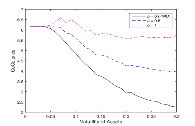
Figure 1: CoCo Prices and asset volatility for different CoCo design parameters

6.2 Asset Volatility, Accounting Noise and CoCo design parameters

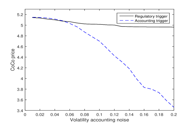
Figure 2: Accounting noise and trigger design

In this subsection we study the impact of changes in asset volatility and accounting noise on CoCo prices as a function of different design parameters.

6.2.1 Asset Volatility shocks

We first look at the price impact of changes in volatility of the underlying asset value process for different CoCo designs. In Figure 1 several CoCo prices are plotted against the volatility of assets $\sigma$, see Equation (4.1). The solid line corresponds to a PWD CoCo. Clearly, the price of a PWD CoCo decreases when assets become more volatile. This is of course as one would expect, as a higher $\sigma$ increases the probability of the principal write-down happening, causing the CoCo price to decrease. The dashed line, corresponding to $\rho=0.5$, shows already that this negative effect from volatility on the CoCo price is weaker when terms of conversion are more favorable to the CoCo investor in that her loss is lower, at least some shares are received after conversion, although not yet enough to compensate for the loss of principal. In the extreme case that shareholders are completely wiped out at conversion, corresponding to the dashed-dotted line, this negative effect is even partially reversed. In this case, the price first increases with volatility as the (now favorable) conversion becomes more likely. However, for higher volatility levels the increasing probability of default and associated costs of bankruptcy push the price down again.

6.2.2 Accounting Noise shocks

We next consider the relationship between accounting noise $\sigma_{\epsilon}$ and the price of a CoCo. In Figure 2, CoCos with a regulatory trigger and CoCos with an accounting based trigger are considered. The book value CoCo is priced by the formula given in Equation (Theorem 4.8 (Price of a PWD CoCo with a sole accounting trigger)); This value is computed using the approximation in Equation (5.5), for which the necessary samples are obtained by using 5.

Figure 2 shows the importance of taking into account the trigger design for the pricing of the CoCo. The increase in accounting volatility has almost no impact on the value of the CoCo with a regulatory trigger (the solid line in Figure 2); but the dashed line shows that the value of CoCos with a trigger that depends on accounting reports, the CoCo price is seriously (and obviously negatively) affected by accounting noise. This is in line with the results of  Duffie and Lando (2001): they find that the default probability increases when the reports become more noisy. In our CoCo setting, this means that the probability of conversion increases when $\sigma_{\epsilon}$ increases, causing the CoCo price to go down. Figure 2 shows that the price of a CoCo with the trigger depending on accounting reports (slotted line) is much more sensitive to accounting noise than the price of a CoCo with a regulatory (PONV) trigger (solid line).

6.2.3 Accounting news and correlation in the accounting report error

Consider next the impact of the correlation coefficient $\kappa$ in the accounting noise error term. In Figure 3 we show the price response of a PWD CoCo to a bad news accounting report. The set up is as follows. After the first report ($Y_{1}=\log 100)$, a second report is issued: $Y_{2}=\log 85$. The conversion trigger is set at $\log 80$, with a PONV trigger type. The plots show a clear and immediate price response to the arrival of the bad news.

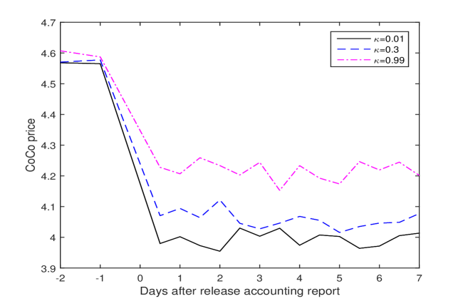
Figure 3: Price response to “bad accounting news” for different values of the autocorrelation parameter $\kappa$.

Interestingly, a clear pattern emerges if the exercise is repeated for different values of the autocorrelation parameter $\kappa$: although the pattern is similar over the entire range from almost no correlation in accounting noise ($\kappa=0.01)$ to almost complete persistence of accounting noise innovations ($\kappa=0.99)$, for higher values of the correlation parameter the price response is more muted. Since the accounting report is known to be contaminated by accounting noise each time a new report is issued, a higher value of $\kappa$ means that more of the past noise arrivals survive in the current one, while at the same time the variance of the accounting noise term $U_{i}$ increases with $\kappa$, as it is, in a stationary regime, proportional to $1/(1-\kappa^{2})$. This in turn lowers the information value of accounting news and explains why a bad (i.e. worse than the previous one) report leads to a smaller negative price response for higher $\kappa:$ the signal is less informative so triggers a smaller price response.

6.2.4 Time lapsed since last accounting report

In Figure 4 we report on a different experiment: we show how different CoCo designs are influenced by time lapsed since the last accounting report. The plot shows the value of three differently structured CoCo’s, each with a different degree of shareholder dilution after conversion as a function of time lapsed since the last accounting report. The black line represents a PWD CoCo where the CoCo is written off upon conversion and no subsequent dilution of the old shareholder takes place; the other two lines represent equity converters, one with partial dilution of the old shareholder ($\rho=0.5)$, the dashed-dotted line, and one where the old shareholder is completely wiped out after conversion $(\rho=1)$, the dashed line.

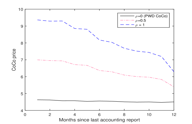
Figure 4: Time since last accounting report.

The plots show very little impact on the PWD CoCo while the two equity converters decline in value as the time since the last accounting report increases. A longer time lapse does not change the asset price dynamics but leads to a higher uncertainty as to where the asset value is at the time of valuation. This is similar to moving more weights in the tails and thus a larger probability of bankruptcy. Since bankruptcy follows conversion, a higher probability of bankruptcy does not influence the PWD, they will then already have lost everything because conversion precedes bankruptcy. But the more shares the CoCo holder receives upon conversion, the more she loses from a subsequent bankruptcy, so the price decline increases more for higher values of the dilution parameter $\rho$.

6.3 Design parameters and CoCo Valuation

Consider next the impact on pricing of the main characteristics of the CoCo design: the trigger level and the number of shares received upon conversion.

6.3.1 The conversion trigger

In Figure 5, the CoCo price is plotted against the conversion trigger for different degrees of dilution. The solid line corresponds to a PWD CoCo, the other lines to CoCos with varying degrees of dilution of the original shareholders upon conversion as specified in the legend.

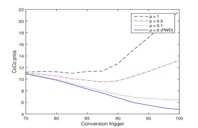
Figure 5: Conversion Trigger

As one would expect, the price of a PWD CoCo (the solid line) is lower for a higher conversion trigger: a higher conversion trigger increases the probability of a principal write-down and its associated loss of principal. However, the other lines show that if conversion terms are more favorable to the CoCo investor, the impact of the trigger level changes: price will increase with the conversion trigger if the dilution ratio favors the CoCo holder enough. In the extreme case that the dilution ratio $\rho$ equals one (the dashed line in Figure 5), the CoCo price goes up with the conversion trigger. For less extreme dilution parameters, this positive effect is weaker, and the corresponding lines are in between the two extremes (no dilution versus complete dilution).

6.3.2 On dilution and Leverage

In Figure 6, the price of a CoCo is plotted against $\Delta$, the number of shares received at conversion per unit of principal, for different values of straight debt in the firm’s capital structure. The case $\Delta=0$ corresponds to a principal write-down CoCo, while $\Delta=\infty$ corresponds to the case in which all of the original shareholders are wiped out at conversion and the CoCo investors are then the only shareholders left. Figure 6 clearly shows that the CoCo price increases with $\Delta$. This is of course as expected, as a higher $\Delta$ means a higher payout at conversion. Furthermore, the figure shows that a CoCo with a conversion into shares has a higher price when there is a lower amount of straight debt issued. Hence the CoCo is more valuable when the firm has a lower leverage. This can also easily be explained, as the CoCo investors receive a fraction of the firm’s equity value at conversion and the equity value is higher in case there are less liabilities.

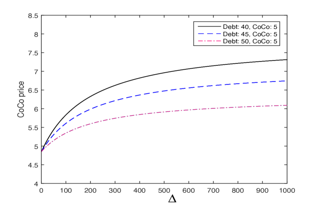
Figure 6: CoCo prices against dilution, for different leverage ratios.

The lines for different leverage converge to the same point on the vertical axis as $\Delta\rightarrow 0;$ for a PWD CoCo, leverage has no impact on the price since both the CoCo and equity are junior to debt. This result does depend on the assumption that the variance of the asset value process is exogenously chosen; if it would be endogenously chosen, higher leverage would lead to more risk taking and a higher variance, which would have an impact on the value of the CoCo even if it has a PWD structure (this point is made in Chan and van Wijnbergen (2016; revised November 2017)).

6.4 Capital structure, CoCos and Risk Taking Incentives

6.4.1 Issuing CoCos to replace straight debt

Consider next the impact of the issuance of CoCos on the capital structure of the bank and, deduced from that, on incentives for shareholders. First consider the case in which straight debt is replaced with CoCos. In Figure 7 we show the change in equity value (on the vertical axis) as a consequence of replacing 5 units of straight debt with 5 units of CoCos, set off against different trigger prices. The different lines correspond to different degrees of the dilution parameter $\rho$, again ranging from 0 to 1 (from no dilution at all to infinite dilution). The solid line and the dotted line indicate that shareholders only benefit from replacing debt with CoCos when the terms of conversion are favorable enough to the shareholders and the trigger is high enough. For low trigger ratios, the conversion possibility becomes very small and the exercise comes down to swapping debt for debt. That actually turns out to have a negative impact on equity values because CoCos then are just a more expensive form of debt so replacing debt with CoCos then actually destroys equity value. As the trigger ratio goes up (move to the right in Figure 7), the probability of getting the benefit of wiping out the CoCo debt at favorable terms becomes more likely and starts to dominate, hence the positive sign for high trigger ratios. Of course that second effect does not take place for highly dilutive CoCos, for low probability of conversion the impact of the debt for CoCo swap is negative, as with non-dilutive CoCo’s. But as the conversion trigger rises and with it the conversion probability, the negative impact of a highly dilutive conversion comes closer, so the price impact turns even more negative. So the dashed line and the dashed-dotted line (highly dilutive cases) show that shareholders have no incentive to swap debt for highly dilutive CoCos, and increasingly less so as the probability of conversion increases with higher trigger levels (academic convention).

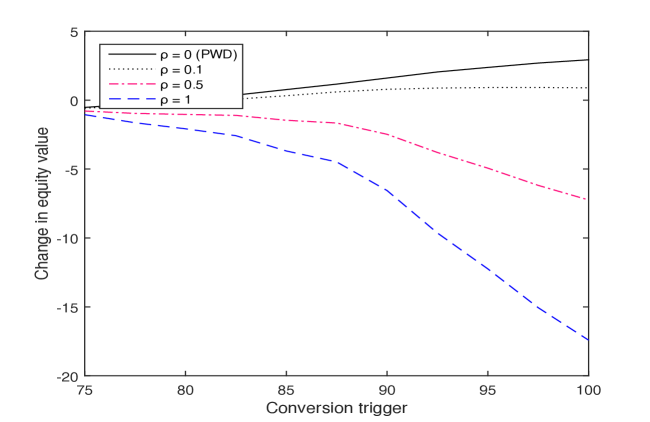
Figure 7: Change in Equity Value when 5 units of debt are replaced with 5 units of CoCo (in market value terms).

6.4.2 Issuing CoCos to replace equity

Consider next a change in capital structure in the other direction, where equity instead of debt is replaced by CoCos. Specifically, we assume a CoCo is issued and the proceeds are used to buy back equity at market value. The consequences on equity values are shown in Figure 8, again for different trigger levels (on the horizontal axis with the different lines representing different degrees of dilution after conversion).

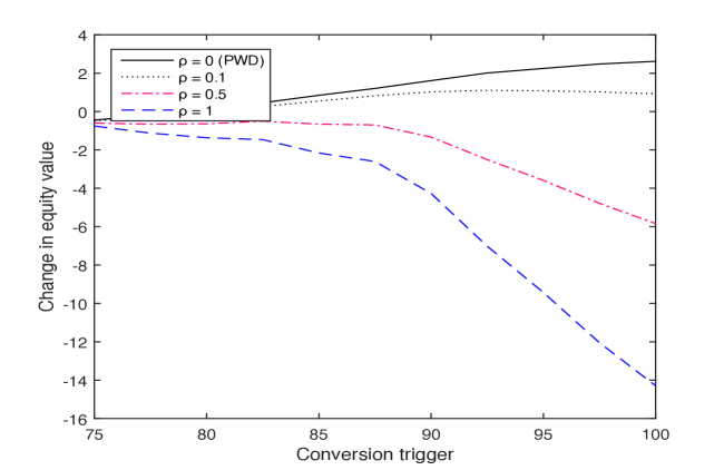
Figure 8: Change in equity value when 5 units of equity are replaced with 5 units of CoCos (in market value)

The pattern is very similar to the debt for CoCo swaps analyzed in Figure 7. Equity holders have a strong incentive to issue PWD CoCos with $\rho=0$ instead of new equity (or even issue PWD CoCos to buy back debt as is done in this policy experiment), since they actually gain on conversion. However for lower trigger ratios the probability of conversion becomes too small, turning CoCos de facto into expensive debt, so the impact on equity value turns negative for low values of the trigger ratio. And equity holders will never want to issue dilutive CoCos ($\rho=1$ is the extreme case with infinite dilution) for any level of the trigger ratio: before conversion these CoCos are an expensive form of debt and after conversion or rather at conversion time equity holders will actually loose out when conversion takes place, making the instrument unambiguously unattractive to shareholders when structured this way. These results may well explain why some 60% of all CoCos are PWD CoCos, cf. Avdiev et al. (2017), instead of the dilutive CoCos favored by the academic literature (Calomiris and Herring (2013) is an early and eloquent example of what is a widely shared view in the academic literature arguing CoCos should be highly dilutive).

6.5 Debt Overhang: on CoCos and Investment Incentives

Debt overhang arises when the firm’s loss absorption capacity has become too low to protect the debtholders from fluctuations in asset values (cf. Merton (1974), Myers (1977)), possibly to the point of arrears having emerged already. One consequence of debt overhang is that investment incentives are reduced for equity holders, since part of the benefits of a new project will in effect have to be shared with the creditors. Even if there are no actual arrears yet, but debt is trading under par, part of the asset value increase will go into increased market value of the debt, at the (partial) expense of a higher market value for equity. In a structural model without CoCos, the shareholders then do not have an incentive to invest exactly at the moment the firm most needs an increase in asset values, i.e. when the firm is near bankruptcy. Almost all of the value of the investment will then be captured by the debt holders, as the value of debt increases when the probability of a bankruptcy is reduced. In which way CoCos interact with a situation with debt overhang is an interesting question; CoCos introduce additional loss absorption capacity which is good for debt holders, but CoCos may also have their own impact on equity values. Debt holders may also profit in another way in that, depending on the design of the CoCos, shareholders may have an increased incentive to make an investment to avoid conversion.

The debt overhang and incentive issue can be looked at within the context of our model by looking at what happens when assets are increased by one unit, financed through one unit of equity (issued at market value). If the total market value of equity goes up by more than one unit, the shareholders would make a profit when they invest, giving them an incentive to do so. However, when equity increases by less than one unit, the investment is not beneficial to shareholders to offset the expense, all or part of the benefits are apparently captured by debt holders. We therefore consider the case in which a new accounting report has just be released, with an asset value, see Equation (4.2), of $Y_{t_{n}}=100$; we can then examine what happens when this asset value increases by one unit. The profit of this investment of one unit is plotted against the conversion trigger in Figure 9.

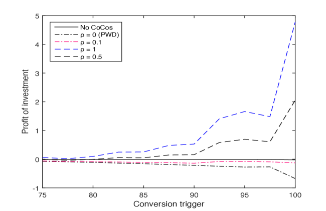
Figure 9: Debt overhang, CoCos and investment incentives

The solid black line is our benchmark case with only straight debt in addition to equity. The simulation shows the impact of debt overhang: without CoCos (the solid line) the shareholders do not make a profit when they invest, they actually suffer a small loss. The dashed-dotted lines show that when the terms of conversion are favorable to shareholders (i.e. CoCo holders loose out upon conversion), the shareholders have even less of an incentive to engage in additional investment, actually worsening the debt overhang problem. The black dashed-dotted line corresponds to the existence of a PWD CoCo in the capital structure of the firm and shows that the PWD CoCo indeed makes the investment incentive for shareholders more negative, especially close to the conversion trigger. So the strongest increase in Debt Overhang is with the CoCos that most favors shareholders, the CoCos with a principal write-down. The same happens to a somewhat lesser degree with CoCos at slightly less non-dilutive terms but still favorable to shareholders. Thus PWD or insufficiently dilutive CoCos are not capable of solving the problem of debt overhang. However, highly dilutive CoCos do strengthen shareholders’ incentives to invest because they want to avoid conversion. See in particular the dashed lines in Figure 9, which correspond to highly dilutive CoCos; clearly such CoCos improve the shareholders’ investment incentives because they wish to avoid conversion. Especially close to the conversion trigger, the shareholders have in this case a substantive incentive to invest in a last attempt to avoid the unfavorable conversion. To summarize, when terms of conversion are beneficial enough to CoCo investors instead of favoring the old shareholders, CoCos are capable of creating more of an investment incentive for the shareholders. However, PWD CoCos and in general less dilutive CoCos actually lead to lower investment incentives and worsen the debt overhang problem when compared to straight debt.

6.6 Coupon payments, the MDA trigger and the Deutsche Bank CoCo scare of February 2016

In the literature it is generally assumed that coupons are paid until conversion. However coupon payments are affected by the so called Maximum Distributable Amount trigger, under which regulators stop the payment of coupons (and dividends) when the firm’s capital value falls below some trigger that is higher than the conversion trigger. Coupon payments can start again when the capital value goes back up and exceeds the trigger value again. This means that in the valuation of a CoCo, we can apply Theorem 4.3.2 and Algorithm 5, but with the coupon term defined as in Equation (4.13). To demonstrate the relevance of the inclusion of this trigger in the valuation of CoCos, we will look at the big price drop that the CoCos of Deutsche Bank suffered at the beginning of 2016. On January 28 Deutsche Bank reported a net loss of 2.1 Billion EUR over the last quarter of 2015. The relevant report furthermore reported for its Risk-Weighted Assets a value of 397 Billion EUR, down from 408 Billion EUR in the previous accounting report. Also, the Common Equity Tier 1 (CET1) ratio, defined as the fraction of the common equity and the risk weighted asset (RWA), fell from 11.5% to 11.1%, primarily reflecting the net loss over the quarter. The information is taken from the Financial Data Supplement 4Q2015, Deutsche Bank (2016), the report that caused a big downward move in the price of the CoCos of Deutsche Bank.

At this time, Deutsche Bank had four different CoCos issued (two in USD, one in EUR, one in GBP, all PWD CoCos). To avoid having to deal with an additional exchange rate risk factor, we will only consider the EUR CoCo. This CoCo’s write-down is triggered when the CET1-ratio hits the level of 5.125% and it pays a coupon of 6%. As is clear from the above, the CET1-ratio did not even come close to the low trigger level. Still, the CoCo price tumbled 19.5% percent within the week after the announcement of the report. Market publications at the time widely argued that this happened out of fear for reaching the MDA trigger and the subsequent cancelling of coupon payments. The model developed in this paper is particularly relevant to analyze this case, as we can include the announcement of a bad accounting report in the valuation, as well as the early cancelling of coupons when the MDA trigger is hit. The precise value of the MDA trigger is not publicly known, so it is not possible to use the real value of the MDA trigger. However, it is still interesting to examine how much of a price drop the model can explain by taking the MDA trigger close to the reported values. Unless stated otherwise, we use the same parameters as in Table 1. Before the bad accounting report arrives, we assume there is one accounting report, with a value $Y_{t_{1}}$= EUR 408 bn. Then the new accounting report arrives, so we now have two accounting reports with values $Y_{t_{1}}$=EUR 408 bn and $Y_{t_{2}}$=EUR 397 bn. The triggers are chosen such that they correspond with CET1 ratios at the moment of the accounting report. That is, we choose $v_{c}$ such that it corresponds to a CET1 ratio of 5.125%. We know the CET1 ratio is 11.1% where RWA is EUR 397 bn, so the total amount of debt (only CoCos and straight debt in the model) is EUR 397 bn $\times$ 0.889 = EUR 352.93 bn. So a CET1 ratio of 5.125% would then correspond to a RWA value of EUR 352.93/(1-0.05125) = EUR 372 bn, which is thus the value of the conversion trigger $v_{c}$. The value of the MDA trigger $v_{cc}$ can be chosen in the same way, a MDA trigger at a CET1 ratio of 10% would correspond to a RWA value of EUR 352.93/(1-0.1) bn = EUR 392 bn. The coupon of the CoCo is $c_{2}$ = 0.06. As the relevant CoCo has a perpetual maturity, we choose the first call date, 10/10/18, as the maturity. Because we assumed that the second accounting report arrives at 01/28/16, t=0 corresponds to 07/28/15. Hence T = 3 + 2/12 + 13/365. In Figure 10 the price change after the announcement of a bad accounting report is illustrated for different choices of the MDA trigger.

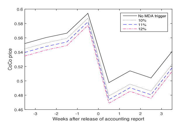
Figure 10: CoCo price after the release of the bad accounting report for different values of the MDA trigger.

The solid line corresponds to the case where the MDA-trigger is not included in the model, in this case only a drop of 14.3% in the CoCo price occurs, when looking at the price just before the release of the accounting report and afterwards. However, if we add the MDA trigger to the model, a stronger negative price change follows. The dashed line corresponds to the case that we take the MDA trigger at 11%, i.e. just beneath the reported CET1 value. This gives a price drop of 18.7%. If we take the MDA trigger to be 10%, the price drops by 17.3%, which is illustrated by the dotted line. However, we have to take the MDA trigger above the reported CET1 ratio of 11.1% to create a price drop of 19.5%, cf. the dashed-dotted line. That is, a price drop of 19.5% corresponds in the model to the situation that the MDA trigger is already breached, which was not the case. However, it is clear that a significant part of the price change is driven by the MDA trigger, not by the conversion trigger. The above illustrates the added value of explicitly incorporating accounting reports into the analysis and taking the MDA trigger into account in the valuation of a CoCo, especially when the MDA trigger is coming close, but the conversion trigger is still far away.

7 Conclusions

CoCos are debt instruments that are written down or converted into equity when the value of the issuing bank becomes too low. CoCos have taken European capital markets by storm. Over 560 bn Euro has been issued over the past five years, with more likely to come. Apparently banks see CoCos as an attractive alternative to issuing new equity when faced with a capital shortage. The academic literature has rapidly developed attempting to analyse and price the new debt instruments, but at the same time a remarkable divergence has opened up between this academic literature and the type of CoCos issued in actual practice. Without exception, the academic literature argues for conversion triggers based on market values instead of accounting ratios. Accordingly, with the exception of Glasserman and Nouri (2012), the asset pricing literature on CoCos has analysed market based conversion triggers only. Yet, at least in the European Union and Switzerland, market based triggers disqualify the instrument as capital under EU regulation, so without a single exception all CoCos issued so far base their conversion trigger on accounting ratios. In addition, they have to keep open the possibility of regulatory intervention when a so called Point of Non-Viability is reached. Moreover, the literature has paid no attention to the triggers in place for suspension of coupon payments, although those triggers have most likely caused most of the recent volatility in CoCo prices. In this paper we bridge the gap between the academic literature and actual practice by explicitly introducing coupon suspension triggers and, arguably more important, explicitly introducing key features of the accounting process in the model which allows us to analyse accounting ratio based conversion triggers and PONV interventions in a meaningful way.

In order to do so we model the basic stochastic process driving asset values as a standard geometric Brownian Motion, as does most of the literature. Where we diverge is in our assumption that the process is not directly observable. Instead information reaches the market based on noisy accounting reports issued at regular but discrete time epochs only. In this way we can take into account differences between accounting values and market values. Our model is based on the premise that the market cannot observe the true asset value process, it only has access to noisy accounting reports which moreover, are only published at discrete moments in time. In this way, the price of CoCos can only be based on the information from the accounting reports, not on the underlying true asset process as this is not observed directly. The model does not lead to closed form solutions for CoCo prices, but Markov Chain Monte Carlo methods are used to compute prices.

The model was remarkably successful in reproducing the price response of CoCos to a widely reported adverse profit warning issued by Deutsche Bank in February 2016. This exercise has shown the importance of incorporating the so called MDA trigger in valuation models, the trigger that governs suspension of coupon payments. Using the model as a tool of analysis yields a rich set of results on the relation between valuation, CoCo design and environment variables such as asset volatility and accounting noise. Moreover, we have shown that CoCos depending on their design have a significant impact on shareholder incentives to take on additional risk or on investment incentives in situations of debt overhang, and interact in interesting ways with the capital structure of the bank issuing them. The various results, such as the attractiveness of PWD CoCos for equity holders, can help explain the design choices made in practice where about 60% of all CoCos issued are of that variety. The explicit incorporation of the accounting process as providing noisy reports on the underlying unobservable firm fundamentals, which are issued at regular but discrete time instants, allows us to analyse CoCo designs based on accounting ratios as well as triggers based on reaching a so called Point of Non-Viability. The relation between risk taking incentives, leverage and CoCo design should be of interest to regulators. We show that CoCos, again depending on their design features, may significantly change the sensitivity of equity values to risk, thereby possibly opening the door to risk arbitrage for given capital requirements, taking into account asset characteristics only, as is the case under the BIS based capital regime.

Appendix A Appendix

In this Appendix, all the mathematical details and proofs that are left out in the main text, are provided.
Proof of Lemma 4.2 $\tilde{f}(t,\cdot,z_{0})$ is defined by

$$\mathbb{P}\left(Z_{t}\in\mathrm{d}x|\tau_{b}>t\right)=\tilde{f}(t,x,z_{0})\mathrm{d}x.$$

By Bayes’ rule we can write

$$\mathbb{P}\left(Z_{t}\in\mathrm{d}x|\tau_{b}>t\right)=\frac{\mathbb{P}\left(Z_{t}\in\mathrm{d}x,\tau_{b}>t\right)}{\mathbb{P}(\tau_{b}>t)}.$$

The denominator of this expression is given by

$$\mathbb{P}(\tau_{b}>t)=1-\pi(t,z_{0}-z_{b})=\Phi\left(\frac{z_{0}-z_{b}+mt}{\sigma\sqrt{t}}\right)-e^{-2m(z_{0}-z_{b})/\sigma^{2}}\Phi\left(\frac{z_{b}-z_{0}+mt}{\sigma\sqrt{t}}\right).$$

In order to compute the numerator, we will rely on the following result by Harrison [1985], which can be found in Section 1.8, Proposition 1. Denote by $X_{t}$ a Brownian motion with drift $\mu$, variance $\sigma^{2}$ and $X_{0}=0$. Furthermore define $M_{t}:=\max\{X_{s}:0\leq s\leq t\}$. Then the joint distribution of $X_{t}$ and $M_{t}$ satisfies

$$\mathbb{P}\left(X_{t}\in\mathrm{d}x,M_{t}\leq y\right)=\frac{1}{\sigma\sqrt{t}}\exp\left(\frac{\mu x}{\sigma^{2}}-\frac{\mu^{2}t}{2\sigma^{2}}\right)\left(\phi\left(\frac{x}{\sigma\sqrt{t}}\right)-\phi\left(\frac{x-2y}{\sigma\sqrt{t}}\right)\right)\mathrm{d}x,$$ (A.1)

where $\phi$ denotes the standard normal density function. Now, denote $X_{t}=-Z_{t}+z_{0}$, which is a Brownian motion with drift $-m$, variance $\sigma^{2}$ and $X_{0}=0$. Furthermore, denote $M_{t}=\max\{X_{s}:0\leq s\leq t\}$. Then Equation (A.1) implies that

$$\mathbb{P}\left(Z_{t}\in\mathrm{d}x,\tau_{b}>t\right) =\mathbb{P}\left(Z_{t}\in\mathrm{d}x,\inf_{0\leq s\leq t}Z_{s}>z_{b}\right)$$

$$=\mathbb{P}\left(X_{t}\in\mathrm{d}(z_{0}-x),M_{t}\leq z_{0}-z_{b}\right)$$

$$=\frac{1}{\sigma\sqrt{t}}\exp\left(\frac{-m(z_{0}-x)}{\sigma^{2}}-\frac{m^{2}t}{2\sigma^{2}}\right)\left(\phi\left(\frac{z_{0}-x}{\sigma\sqrt{t}}\right)-\phi\left(\frac{-z_{0}-x+2z_{b}}{\sigma\sqrt{t}}\right)\right)\mathrm{d}x.$$ (A.2)

So we conclude that

$$\tilde{f}(t,x,z_{0})=\frac{1}{\sigma\sqrt{t}}\frac{\exp\left(\frac{-m(z_{0}-x)}{\sigma^{2}}-\frac{m^{2}t}{2\sigma^{2}}\right)\left(\phi\left(\frac{z_{0}-x}{\sigma\sqrt{t}}\right)-\phi\left(\frac{-z_{0}-x+2z_{b}}{\sigma\sqrt{t}}\right)\right)}{\Phi\left(\frac{z_{0}-z_{b}+mt}{\sigma\sqrt{t}}\right)-e^{-2m(z_{0}-z_{b})/\sigma^{2}}\Phi\left(\frac{z_{b}-z_{0}+mt}{\sigma\sqrt{t}}\right)}.$$

$\square$
Proof of Theorem 4.3.1 Recall that the CoCo price was written as

$$C(t)=Pe^{-r(T-t)}p_{c}(t,T)+cP\int_{t}^{T}e^{-r(u-t)}p_{c}(t,u)\mathrm{d}u-RP\int_{t}^{T}e^{-r(u-t)}p_{c}(t,\mathrm{d}u).$$ (A.3)

The integral in this last term can be written as

$$\int_{t}^{T}e^{-r(u-t)}p_{c}(t,\mathrm{d}u) =\int_{t}^{T}e^{-r(u-t)}\frac{\partial}{\partial u}p_{c}(t,u)\mathrm{d}u$$

$$=\int_{t}^{T}e^{-r(u-t)}\int_{z_{c}}^{\infty}\frac{\partial}{\partial u}(1-\pi(u-t,x-z_{c}))f(t,x,\omega)\mathrm{d}x\mathrm{d}u$$

$$=\int_{z_{c}}^{\infty}f(t,x,\omega)\int_{t}^{T}e^{-r(u-t)}\frac{\partial}{\partial u}(1-\pi(u-t,x-z_{c}))\mathrm{d}u\mathrm{d}x$$

$$=\int_{z_{c}}^{\infty}f(t,x,\omega)I(x)\mathrm{d}x,$$

where

$$I(x)=\int_{t}^{T}e^{-r(u-t)}\frac{\partial}{\partial u}(1-\pi(u-t,x-z_{c}))\mathrm{d}u.$$

Furthermore, the integral in the second term of Equation (A.3) can be written as

$$\int_{t}^{T}e^{-r(u-t)}p_{c}(t,u)\mathrm{d}u =\int_{t}^{T}e^{-r(u-t)}\int_{z_{c}}^{\infty}(1-\pi(u-t,x-z_{c}))f(t,x,\omega)\mathrm{d}x\mathrm{d}u$$

$$=\int_{z_{c}}^{\infty}f(t,x,\omega)\int_{t}^{T}e^{-r(u-t)}(1-\pi(u-t,x-z_{c}))\mathrm{d}u\mathrm{d}x$$

$$=\int_{z_{c}}^{\infty}f(t,x,\omega)\tilde{I}(x)\mathrm{d}x,$$

where

$$\tilde{I}(x) =\int_{t}^{T}e^{-r(u-t)}(1-\pi(u-t,x-z_{c}))\mathrm{d}u$$

$$=\left[-\frac{1}{r}e^{-r(u-t)}(1-\pi(u-t,x-z_{c}))\right]_{u=t}^{T}+\frac{1}{r}I(x)$$

$$=-\frac{1}{r}e^{-r(T-t)}(1-\pi(T-t,x-z_{c}))+\frac{1}{r}+\frac{1}{r}I(x).$$

Putting the above together allows us to write the CoCo price $C(t)$ as a single integral, weighted by the density $f(t,x)$, as follows

$$C(t) =\int_{z_{c}}^{\infty}\left(Pe^{-r(T-t)}(1-\pi(T-t,x-z_{c}))+cP\tilde{I}(x)-RPI(x)\right)f(t,xa)\mathrm{d}x$$

$$=\int_{z_{c}}^{\infty}\left(\frac{r-c}{r}Pe^{-r(T-t)}(1-\pi(T-t,x-z_{c}))+\frac{c}{r}P+\left(\frac{cP}{r}-RP\right)I(x)\right)f(t,x)\mathrm{d}x.$$

It now remains to find an analytical expression for $I(x)$. First consider

$$\frac{\partial}{\partial u}(1-\pi(u-t,x-z_{c}))$$

$$\quad=\frac{\partial}{\partial u}\left(\Phi\left(\frac{x-z_{c}+m(u-t)}{\sigma\sqrt{u-t}}\right)-e^{-2m(x-z_{c})/\sigma^{2}}\Phi\left(\frac{-(x-z_{c})+m(u-t)}{\sigma\sqrt{u-t}}\right)\right)$$

$$\quad=\phi\left(\frac{x-z_{c}+m(u-t)}{\sigma\sqrt{u-t}}\right)\left(\frac{m}{2\sigma\sqrt{u-t}}-\frac{x-z_{c}}{2\sigma(u-t)^{3/2}}\right)$$

$$\quad\quad-e^{-2m(x-z_{c})/\sigma^{2}}\phi\left(\frac{-(x-z_{c})+m(u-t)}{\sigma\sqrt{u-t}}\right)\left(\frac{m}{2\sigma\sqrt{u-t}}+\frac{x-z_{c}}{2\sigma(u-t)^{3/2}}\right)$$

$$\quad=\frac{z_{c}-x}{\sigma(u-t)^{3/2}}\phi\left(\frac{x-z_{c}+m(u-t)}{\sigma\sqrt{u-t}}\right),$$

which implies

$$I(x) =\int_{t}^{T}e^{-r(u-t)}\frac{z_{c}-x}{\sigma(u-t)^{3/2}}\frac{1}{\sqrt{2\pi}}\exp\left(-\frac{(x-z_{c}+m(u-t))^{2}}{2\sigma^{2}(u-t)}\right)\mathrm{d}u$$

$$=\frac{z_{c}-x}{\sqrt{2\pi\sigma^{2}}}\exp\left(-\frac{m(x-z_{c})}{\sigma^{2}}\right)\int_{0}^{T-t}e^{-ru}\frac{1}{u^{3/2}}\exp\left(-\frac{(x-z_{c})^{2}}{2\sigma^{2}u}-\frac{m^{2}u}{2\sigma^{2}}\right)\mathrm{d}u$$

$$=\frac{z_{c}-x}{\sqrt{2\pi\sigma^{2}}}\exp\left(-\frac{m(x-z_{c})}{\sigma^{2}}\right)\int_{0}^{T-t}\frac{1}{u^{3/2}}\exp\left(-\frac{(x-z_{c})^{2}}{2\sigma^{2}}\frac{1}{u}-\left(\frac{m^{2}}{2\sigma^{2}}+r\right)u\right)\mathrm{d}u$$

$$=2\frac{z_{c}-x}{\sqrt{2\pi\sigma^{2}}}\exp\left(-\frac{m(x-z_{c})}{\sigma^{2}}\right)\int_{(T-t)^{-1/2}}^{\infty}\exp\left(-Av^{2}-B\frac{1}{v^{2}}\right)\mathrm{d}v,$$ (A.4)

where the last line follows by substitution of $v=u^{-1/2}$ and by setting

$$A=\frac{(x-z_{c})^{2}}{2\sigma^{2}},\leavevmode\nobreak\ B=\frac{m^{2}}{2\sigma^{2}}+r.$$

Now, by noting that $(Av^{2}+B/v^{2})=(\sqrt{A}v-\sqrt{B}/v)^{2}+2\sqrt{AB}$, as well as $(Av^{2}+B/v^{2})=(\sqrt{A}v+\sqrt{B}/v)^{2}-2\sqrt{AB}$, the remaining integral can be evaluated, by doing the substitutions $u=\sqrt{A}v-\sqrt{B}/v$ and $u=\sqrt{A}v+\sqrt{B}/v$, as follows

$$\int_{(T-t)^{-1/2}}^{\infty}\exp\left(-Av^{2}-B\frac{1}{v^{2}}\right)\mathrm{d}v$$

$$=\frac{1}{2\sqrt{A}}\int_{(T-t)^{-1/2}}^{\infty}\exp\left(-(\sqrt{A}v-\sqrt{B}/v)^{2}-2\sqrt{AB}\right)(\sqrt{A}+\sqrt{B}\frac{1}{v^{2}})\mathrm{d}v$$

$$\leavevmode\nobreak\ \leavevmode\nobreak\ \leavevmode\nobreak\ +\frac{1}{2\sqrt{A}}\int_{(T-t)^{-1/2}}^{\infty}\exp\left(-(\sqrt{A}v+\sqrt{B}/v)^{2}+2\sqrt{AB}\right)(\sqrt{A}-\sqrt{B}\frac{1}{v^{2}})\mathrm{d}v$$

$$=\frac{1}{2\sqrt{A}}e^{-2\sqrt{AB}}\int_{\sqrt{A/(T-t)}-\sqrt{B(T-t)}}^{\infty}e^{-u^{2}}\mathrm{d}u$$

$$\leavevmode\nobreak\ \leavevmode\nobreak\ \leavevmode\nobreak\ +\frac{1}{2\sqrt{A}}e^{2\sqrt{AB}}\int_{\sqrt{A/(T-t)}+\sqrt{B(T-t)}}^{\infty}e^{-u^{2}}\mathrm{d}u$$

$$=\frac{\sqrt{\pi}}{4\sqrt{A}}\left(e^{-2\sqrt{AB}}\operatorname{erfc}\left(\sqrt{A/(T-t)}-\sqrt{B(T-t)}\right)\right.$$

$$\leavevmode\nobreak\ \leavevmode\nobreak\ \leavevmode\nobreak\ +\left.e^{2\sqrt{AB}}\operatorname{erfc}\left(\sqrt{A/(T-t)}+\sqrt{B(T-t)}\right)\right),$$ (A.5)

where $\operatorname{erfc}(x)$ is the complementary error function, which is defined by

$$\operatorname{erfc}(x):=\frac{2}{\sqrt{\pi}}\int_{x}^{\infty}e^{-u^{2}}\mathrm{d}u$$

and satisfies

$$\frac{1}{2}\operatorname{erfc}(x/\sqrt{2})=1-\Phi(x).$$

Combining Equations (A) and (A) and substituting back the expressions for $A$ and $B$, finally leads to the expression for $I(x)$:

$$I(x) =2\frac{z_{c}-x}{\sqrt{2\pi\sigma^{2}}}\exp\left(-\frac{m(x-z_{c})}{\sigma^{2}}\right)\int_{(T-t)^{-1/2}}^{\infty}\exp\left(-Av^{2}-B\frac{1}{v^{2}}\right)\mathrm{d}v$$

$$=\exp\left(-\frac{m(x-z_{c})}{\sigma^{2}}\right)\left(-e^{-2\sqrt{AB}}\frac{1}{2}\operatorname{erfc}\left(\sqrt{A/(T-t)}-\sqrt{B(T-t)}\right)\right.$$

$$\leavevmode\nobreak\ \leavevmode\nobreak\ \leavevmode\nobreak\ -\left.e^{2\sqrt{AB}}\frac{1}{2}\operatorname{erfc}\left(\sqrt{A/(T-t)}+\sqrt{B(T-t)}\right)\right)$$

$$=\exp\left(-\frac{m(x-z_{c})+(x-z_{c})\sqrt{m^{2}+2r\sigma^{2}}}{\sigma^{2}}\right)\left(\Phi\left(\frac{x-z_{c}-\sqrt{m^{2}+2r\sigma^{2}}(T-t)}{\sigma\sqrt{T-t}}\right)-1\right)$$

$$\leavevmode\nobreak\ \leavevmode\nobreak\ \leavevmode\nobreak\ +\exp\left(-\frac{m(x-z_{c})-(x-z_{c})\sqrt{m^{2}+2r\sigma^{2}}}{\sigma^{2}}\right)\left(\Phi\left(\frac{x-z_{c}+\sqrt{m^{2}+2r\sigma^{2}}(T-t)}{\sigma\sqrt{T-t}}\right)-1\right).$$ (A.6)

$\square$
Proof of Theorem 4.3.2 The market price of the CoCos is given by

$$C(t) =\mathbb{E}\left(P_{2}e^{-r(T-t)}\mathbf{1}_{\{\tau_{c}>T\}}|\mathcal{H}_{t}\right)+\mathbb{E}\left(\int_{t}^{T}c_{2}P_{2}e^{-r(u-t)}\mathbf{1}_{\{\tau_{c}>u\}}\mathrm{d}u|\mathcal{H}_{t}\right)$$

$$\leavevmode\nobreak\ \leavevmode\nobreak\ \leavevmode\nobreak\ +\mathbb{E}\left(\frac{\Delta P_{2}}{\Delta P_{2}+1}E^{PC}(\tau_{c})e^{-r(\tau_{c}-t)}\mathbf{1}_{\{\tau_{c}\leq T\}}|\mathcal{H}_{t}\right).$$ (A.7)

The first two terms together, are captured in the integral

$$\int_{z_{c}}^{\infty}h_{0}(x)f(t,x)\mathrm{d}x,$$

as is clear from taking $R=0$ in the PWD case, cf. Theorem 4.3.1.
Recall that the third term in Equation (A) was written as

$$\mathbb{E}\left(\frac{\Delta P_{2}}{\Delta P_{2}+1}E^{PC}(\tau_{c})e^{-r(\tau_{c}-t)}\mathbf{1}_{\{\tau_{c}\leq T\}}|\mathcal{H}_{t}\right)$$

$$=\frac{\Delta P_{2}}{\Delta P_{2}+1}e^{z_{c}}\int_{t}^{T}e^{-r(u-t)}\mathbb{P}(\tau_{c}\in\mathrm{d}u|\tau_{c}>t,Y^{(n)})$$

$$\leavevmode\nobreak\ \leavevmode\nobreak\ \leavevmode\nobreak\ -\frac{\Delta P_{2}c_{1}P_{1}}{\Delta P_{2}+1}\int_{t}^{\infty}e^{-r(u-t)}\mathbb{P}(\tau_{c}\leq T\wedge u,\tau_{b}>u|\tau_{c}>t,Y^{(n)})\mathrm{d}u$$

$$\leavevmode\nobreak\ \leavevmode\nobreak\ \leavevmode\nobreak\ -\frac{\Delta P_{2}}{\Delta P_{2}+1}e^{z_{b}}\int_{t}^{\infty}e^{-r(u-t)}\mathbb{P}(\tau_{c}\leq T,\tau_{b}\in\mathrm{d}u|\tau_{c}>t,Y^{(n)}).$$ (A.8)

Note that the first integral in this equation is already computed in the proof of Theorem 4.3.1 and given by

$$e^{z_{c}}\int_{t}^{T}e^{-r(u-t)}\mathbb{P}(\tau_{c}\in\mathrm{d}u|\tau_{c}>t,Y^{(n)})=-e^{z_{c}}\int_{z_{c}}^{\infty}f(t,x)I(x)\mathrm{d}x,$$ (A.9)

where $I(x)$ is given by Equation (A).
To compute the other integrals in Equation (A), it is sufficient to find expressions for

$$\mathbb{P}(\tau_{c}\leq T,\tau_{b}>u|\tau_{c}>t,Y^{(n)}=y^{(n)})\text{ and }\mathbb{P}(\tau_{c}\leq u,\tau_{b}>u|\tau_{c}>t,Y^{(n)}=y^{(n)}).$$

In order to find expressions for this joint probabilities, we first need the following lemma.

• The joint probability $\gamma(x,y,z,t_{1},t_{2})$ that $Z$, starting from $x$, does not hit $z$ before time $t_{1}$ but does hit $y$ before time $t_{2}$, is for $x>y>z$ given by

  $$\gamma(x,y,z,t_{1},t_{2}) =\mathbb{P}(\inf_{0\leq s\leq t_{1}}Z_{s}>z,\inf_{0\leq s\leq t_{2}}Z_{s}\leq y)$$

  $$=\left\{\begin{matrix}\pi(t_{2},x-y)-\pi(t_{1},x-z)&\text{ for }t_{1}\leq t_{2},\\ 1-\pi(t_{1},x-z)-\int_{y}^{\infty}(1-\pi(t_{1}-t_{2},\tilde{z}-z))\hat{f}(x,y,\tilde{z},t_{2})\mathrm{d}\tilde{z}&\text{ for }t_{1}>t_{2},\end{matrix}\right.$$

  where

  $$\hat{f}(x,y,\tilde{z},t_{2})=\frac{1}{\sigma\sqrt{t_{2}}}\exp\left(\frac{-m(x-\tilde{z})}{\sigma^{2}}-\frac{m^{2}t_{2}}{2\sigma^{2}}\right)\left(\phi\left(\frac{x-\tilde{z}}{\sigma\sqrt{t_{2}}}\right)-\phi\left(\frac{-x-\tilde{z}+2y}{\sigma\sqrt{t_{2}}}\right)\right)$$ (A.10)

Proof.

• For $t_{1}\leq t_{2}$, we can write

  $$\mathbb{P}(\inf_{0\leq s\leq t_{1}}Z_{s}>z,\inf_{0\leq s\leq t_{2}}Z_{s}\leq y) =\mathbb{P}(\inf_{0\leq s\leq t_{2}}Z_{s}\leq y)-\mathbb{P}(\inf_{0\leq s\leq t_{1}}Z_{s}\leq z,\inf_{0\leq s\leq t_{2}}Z_{s}\leq y)$$

  $$=\mathbb{P}(\inf_{0\leq s\leq t_{2}}Z_{s}\leq y)-\mathbb{P}(\inf_{0\leq s\leq t_{1}}Z_{s}\leq z)$$

  $$=\pi(t_{2},x-y)-\pi(t_{1},x-z).$$

• For $t_{1}>t_{2}$, note that

  $$\mathbb{P}(\inf_{0\leq s\leq t_{1}}Z_{s}>z,\inf_{0\leq s\leq t_{2}}Z_{s}\leq y) =\mathbb{P}(\inf_{0\leq s\leq t_{1}}Z_{s}>z)-\mathbb{P}(\inf_{0\leq s\leq t_{1}}Z_{s}>z,\inf_{0\leq s\leq t_{2}}Z_{s}>y)$$

  $$=1-\pi(t_{1},x-z)-\mathbb{P}(\inf_{0\leq s\leq t_{1}}Z_{s}>z,\inf_{0\leq s\leq t_{2}}Z_{s}>y),$$

  where

  $$\mathbb{P}(\inf_{0\leq s\leq t_{1}}Z_{s}>z,\inf_{0\leq s\leq t_{2}}Z_{s}>y)$$

  $$\quad=\int_{y}^{\infty}\mathbb{P}\left(\inf_{t_{2}\leq s\leq t_{1}}Z_{s}>z,\inf_{0\leq s\leq t_{2}}Z_{s}>y|Z_{t_{2}}=\tilde{z}\right)\mathbb{P}(Z_{t_{2}}\in\mathrm{d}\tilde{z})$$

  $$\quad=\int_{y}^{\infty}\mathbb{P}\left(\inf_{t_{2}\leq s\leq t_{1}}Z_{s}-Z_{t_{2}}>z-\tilde{z}\right)\mathbb{P}(\inf_{0\leq s\leq t_{2}}Z_{s}>y,Z_{t_{2}}\in\mathrm{d}\tilde{z})$$

  $$\quad=\int_{y}^{\infty}\mathbb{P}\left(\inf_{0\leq s\leq t_{1}-t_{2}}Z_{s}>z-\tilde{z}+x\right)\mathbb{P}(\inf_{0\leq s\leq t_{2}}Z_{s}>y,Z_{t_{2}}\in\mathrm{d}\tilde{z})$$

  $$\quad=\int_{y}^{\infty}(1-\pi(t_{1}-t_{2},\tilde{z}-z))\mathbb{P}(\inf_{0\leq s\leq t_{2}}Z_{s}>y,Z_{t_{2}}\in\mathrm{d}\tilde{z}),$$

  where is used that $Z$ has independent and stationary increments.
  Now the result follows by noting that by a modification of Equation (A) to the current setting, it holds that

$$\mathbb{P}(\inf_{0\leq s\leq t_{2}}Z_{s}>y,Z_{t_{2}}\in\mathrm{d}\tilde{z})=\hat{f}(x,y,\tilde{z},t_{2})\mathrm{d}\tilde{z}.$$

∎

Now the desired probabilities are, in analogy to Equation (4.8), given by

$$\mathbb{P}(\tau_{c}\leq T,\tau_{b}>u|\tau_{c}>t,Y^{(n)}=y^{(n)})=\int_{z_{c}}^{\infty}\gamma(x,z_{c},z_{b},u-t,T-t)f(t,x)\mathrm{d}x$$

and

$$\mathbb{P}(\tau_{c}\leq u,\tau_{b}>u|\tau_{c}>t,Y^{(n)}=y^{(n)})=\int_{z_{c}}^{\infty}\gamma(x,z_{c},z_{b},u-t,u-t)f(t,x)\mathrm{d}x.$$

Recall that the objective was to compute the last two integrals in Equation (A). Let us first consider the second one, that is

$$-\int_{t}^{\infty}e^{-r(u-t)}\mathbb{P}(\tau_{c}\leq T,\tau_{b}\in\mathrm{d}u|\tau_{c}>t,Y^{(n)}) =\int_{t}^{\infty}e^{-r(u-t)}\frac{\partial}{\partial u}\mathbb{P}(\tau_{c}\leq T,\tau_{b}>u|\tau_{c}>t,Y^{(n)})\mathrm{d}u$$

$$=(\mathrm{I})+(\mathrm{II}),$$

where

$$(\mathrm{I}) =\int_{t}^{T}e^{-r(u-t)}\frac{\partial}{\partial u}\mathbb{P}(\tau_{c}\leq T,\tau_{b}>u|\tau_{c}>t,Y^{(n)})\mathrm{d}u$$

$$=\int_{z_{c}}^{\infty}f(t,x)\int_{t}^{T}e^{-r(u-t)}\frac{\partial}{\partial u}\gamma(x,z_{c},z_{b},u-t,T-t)\mathrm{d}u\mathrm{d}x$$

$$=\int_{z_{c}}^{\infty}f(t,x)\int_{t}^{T}e^{-r(u-t)}\frac{\partial}{\partial u}(-\pi(u-t,x-z_{b}))\mathrm{d}u\mathrm{d}x$$

$$=\int_{z_{c}}^{\infty}f(t,x)I_{b}(x)\mathrm{d}x,$$

in which

$$I_{b}(x) =\int_{t}^{T}e^{-r(u-t)}\frac{\partial}{\partial u}(-\pi(u-t,x-z_{b}))\mathrm{d}u$$

$$=\exp\left(-\frac{m(x-z_{b})+(x-z_{b})\sqrt{m^{2}+2r\sigma^{2}}}{\sigma^{2}}\right)\left(\Phi\left(\frac{x-z_{b}-\sqrt{m^{2}+2r\sigma^{2}}(T-t)}{\sigma\sqrt{T-t}}\right)-1\right)$$

$$\leavevmode\nobreak\ \leavevmode\nobreak\ \leavevmode\nobreak\ +\exp\left(-\frac{m(x-z_{b})-(x-z_{b})\sqrt{m^{2}+2r\sigma^{2}}}{\sigma^{2}}\right)\left(\Phi\left(\frac{x-z_{b}+\sqrt{m^{2}+2r\sigma^{2}}(T-t)}{\sigma\sqrt{T-t}}\right)-1\right),$$ (A.11)

which follows from Equation (A), by replacing $z_{c}$ by $z_{b}$. Furthermore, we have

$$(\mathrm{II}) =\int_{T}^{\infty}e^{-r(u-t)}\frac{\partial}{\partial u}\mathbb{P}(\tau_{c}\leq T,\tau_{b}>u|\tau_{c}>t,Y^{(n)})\mathrm{d}u$$

$$=\int_{z_{c}}^{\infty}f(t,x)\int_{T}^{\infty}e^{-r(u-t)}\frac{\partial}{\partial u}\gamma(x,z_{c},z_{b},u-t,T-t)\mathrm{d}u\mathrm{d}x$$

$$=\int_{z_{c}}^{\infty}f(t,x)\int_{T}^{\infty}e^{-r(u-t)}\frac{\partial}{\partial u}(-\pi(u-t,x-z_{b}))\mathrm{d}u\mathrm{d}x$$

$$\leavevmode\nobreak\ \leavevmode\nobreak\ \leavevmode\nobreak\ -\int_{z_{c}}^{\infty}\int_{z_{c}}^{\infty}f(t,x)\hat{f}(x,z_{c},\tilde{z},T-t)\int_{T}^{\infty}e^{-r(u-t)}\frac{\partial}{\partial u}(1-\pi(u-T,\tilde{z}-z_{b}))\mathrm{d}u\mathrm{d}\tilde{z}\mathrm{d}x$$

$$=\int_{z_{c}}^{\infty}f(t,x)(J_{b}(x)-I_{b}(x))\mathrm{d}x$$

$$\leavevmode\nobreak\ \leavevmode\nobreak\ \leavevmode\nobreak\ -\int_{z_{c}}^{\infty}\int_{z_{c}}^{\infty}f(t,x)\hat{f}(x,z_{c},\tilde{z},T-t)e^{-r(T-t)}J_{b}(\tilde{z},T)\mathrm{d}\tilde{z}\mathrm{d}x,$$

where

$$J_{b}(x) =\int_{t}^{\infty}e^{-r(u-t)}\frac{\partial}{\partial u}(1-\pi(u-t,x-z_{b}))\mathrm{d}u$$

$$=-\exp\left(-\frac{m(x-z_{b})+(x-z_{b})\sqrt{m^{2}+2r\sigma^{2}}}{\sigma^{2}}\right),$$ (A.12)

where the last line follows by taking $T\to\infty$ in Equation (A). This leaves us with an expression for the last integral in Equation (A).
Similarly, the other integral satisfies

$$\int_{t}^{\infty}e^{-r(u-t)}\mathbb{P}(\tau_{c}\leq T\wedge u,\tau_{b}>u|\tau_{c}>t,Y^{(n)})\mathrm{d}u =(\mathrm{III})+(\mathrm{IV}),$$

where

$$(\mathrm{III}) =\int_{t}^{T}e^{-r(u-t)}\mathbb{P}(\tau_{c}\leq u,\tau_{b}>u|\tau_{c}>t,Y^{(n)})\mathrm{d}u$$

$$=\int_{z_{c}}^{\infty}f(t,x)\int_{t}^{T}e^{-r(u-t)}\gamma(x,z_{c},z_{b},u-t,u-t)\mathrm{d}u\mathrm{d}x$$

$$=\int_{z_{c}}^{\infty}f(t,x)\int_{t}^{T}e^{-r(u-t)}(\pi(u-t,x-z_{c})-\pi(u-t,x-z_{b}))\mathrm{d}u\mathrm{d}x$$

$$=\int_{z_{c}}^{\infty}f(t,x)(\tilde{I}_{b}(x)-\tilde{I}(x))\mathrm{d}x$$

in which $\tilde{I}(x)$ is defined in the proof Theorem 4.3.1 and $\tilde{I}_{b}(x)$ is equivalently defined as

$$\tilde{I}_{b}(x) =\int_{t}^{T}e^{-r(u-t)}(1-\pi(u-t,x-z_{b}))\mathrm{d}u$$

$$=\left[-\frac{1}{r}e^{-r(u-t)}(1-\pi(u-t,x-z_{b}))\right]_{u=t}^{T}+\frac{1}{r}I_{b}(x)$$

$$=-\frac{1}{r}e^{-r(T-t)}(1-\pi(T-t,x-z_{b}))+\frac{1}{r}+\frac{1}{r}I_{b}(x).$$ (A.13)

Furthermore, we have

$$(\mathrm{IV}) =\int_{T}^{\infty}e^{-r(u-t)}\mathbb{P}(\tau_{c}\leq T,\tau_{b}>u|\tau_{c}>t,Y^{(n)})\mathrm{d}u$$

$$=\int_{z_{c}}^{\infty}\int_{T}^{\infty}e^{-r(u-t)}\gamma(x,z_{c},z_{b},u-t,T-t)\mathrm{d}u\mathrm{d}x$$

$$=\int_{z_{c}}^{\infty}f(t,x)\int_{T}^{\infty}e^{-r(u-t)}(1-\pi(u-t,x-z_{b}))\mathrm{d}u\mathrm{d}x$$

$$\leavevmode\nobreak\ \leavevmode\nobreak\ \leavevmode\nobreak\ -\int_{z_{c}}^{\infty}\int_{z_{c}}^{\infty}f(t,x)\hat{f}(x,z_{c},\tilde{z},T-t)\int_{T}^{\infty}e^{-r(u-t)}(1-\pi(u-T,\tilde{z}-z_{b}))\mathrm{d}u\mathrm{d}\tilde{z}\mathrm{d}x$$

$$=\int_{z_{c}}^{\infty}f(t,x)(\tilde{J}_{b}(x)-\tilde{I}_{b}(x))\mathrm{d}x$$

$$\leavevmode\nobreak\ \leavevmode\nobreak\ \leavevmode\nobreak\ -\int_{z_{c}}^{\infty}\int_{z_{c}}^{\infty}f(t,x)\hat{f}(x,z_{c},\tilde{z},T-t)e^{-r(T-t)}\tilde{J}_{b}(\tilde{z})\mathrm{d}\tilde{z}\mathrm{d}x,$$

in which

$$\tilde{J}_{b}(x) =\int_{t}^{\infty}e^{-r(u-t)}(1-\pi(u-t,x-z_{b}))\mathrm{d}u$$

$$=\left[-\frac{1}{r}(1-\pi(u-t,x-z_{b})\right]_{u=t}^{\infty}+\frac{1}{r}J_{b}(x)$$

$$=\frac{1}{r}+\frac{1}{r}J_{b}(x).$$ (A.14)

Putting all the above together leads to an expression for the last two integrals in Equation (A), given by

$$-c_{1}P_{1}\int_{t}^{\infty}e^{-r(u-t)}\mathbb{P}(\tau_{c}\leq T\wedge u,\tau_{b}>u|\tau_{c}>t,Y^{(n)})\mathrm{d}u$$

$$\quad-e^{z_{b}}\int_{t}^{\infty}e^{-r(u-t)}\mathbb{P}(\tau_{c}\leq T,\tau_{b}\in\mathrm{d}u|\tau_{c}>t,Y^{(n)})$$

$$\quad=e^{z_{b}}((I)+(II))-c_{1}P_{1}((III)+(IV))$$

$$\quad=\int_{z_{c}}^{\infty}f(t,x)\left(e^{z_{b}}J_{b}(x)+c_{1}P_{1}\tilde{I}(x)-c_{1}P_{1}\tilde{J}_{b}(x)\right)\mathrm{d}x$$

$$\quad\quad+\int_{z_{c}}^{\infty}\int_{z_{c}}^{\infty}f(t,x)\hat{f}(x,z_{c},\tilde{z},T-t)e^{-r(T-t)}(c_{1}P_{1}\tilde{J}_{b}(\tilde{z})-e^{z_{b}}J_{b}(\tilde{z}))\mathrm{d}\tilde{z}\mathrm{d}x.$$ (A.15)

Finally, by combining Equations (A), (A.9) and (A), it follows that the third term in Equation (4.3.2), i.e.

$$\mathbb{E}\left(\frac{\Delta P_{2}}{\Delta P_{2}+1}E^{PC}(\tau_{c})e^{-r(\tau_{c}-t)}\mathbf{1}_{\{\tau_{c}\leq T\}}|\mathcal{H}_{t}\right),$$

is given by

$$\int_{z_{c}}^{\infty}f(t,x)h_{1}(x)\mathrm{d}x+\int_{z_{c}}^{\infty}\int_{z_{c}}^{\infty}f(t,x)\hat{f}(x,z_{c},\tilde{z},T-t)h_{2}(\tilde{z})\mathrm{d}\tilde{z}\mathrm{d}x,$$ (A.16)

where

$$h_{1}(x)=\frac{\Delta P_{2}}{\Delta P_{2}+1}\left(e^{z_{b}}J_{b}(x)+c_{1}P_{1}\tilde{I}(x)-c_{1}P_{1}\tilde{J}_{b}(x)-e^{z_{c}}I(x)\right),$$

$$h_{2}(\tilde{z})=\frac{\Delta P_{2}}{\Delta P_{2}+1}e^{-r(T-t)}(c_{1}P_{1}\tilde{J}_{b}(\tilde{z})-e^{z_{b}}J_{b}(\tilde{z})).$$

$\square$
Proof of Proposition 4.3.3 Denote by $\Delta t$ the time between two successive accounting reports and recall from section 4.1 the notation $Y_{i}=Y_{t_{i}},Z_{i}=Z_{t_{i}},U_{i}=U_{t_{i}}$ and that $Y_{i}=Z_{i}+U_{i}$, where

$$U_{i}=\kappa U_{i-1}+\epsilon_{i},$$

for some fixed $\kappa\in\mathbb{R}$ and independent and identically distributed $\epsilon_{1},\epsilon_{2},\dots$, which have a normal distribution with mean $\mu_{\epsilon}$ and variance $\sigma_{\epsilon}^{2}$, and are independent of $Z$. This allows us to write, for $i=1,2,\dots$

$$\left(\begin{matrix}Y_{n+i}\\ \vdots\\ Y_{n+1}\end{matrix}\right) =M\left(\begin{matrix}Z_{n+i}-Z_{n+i-1}\\ \vdots\\ Z_{n+1}-Z_{n}\\ \epsilon_{n+i}\\ \vdots\\ \epsilon_{n+1}\end{matrix}\right)+\left(\begin{matrix}\kappa^{i}\\ \vdots\\ \kappa\end{matrix}\right)Y_{n}+\left(\begin{matrix}1-\kappa^{i}\\ \vdots\\ 1-\kappa\end{matrix}\right)Z_{n},$$

where $M$ denotes the $(i\times 2i)$-matrix defined by

$$M=\overbrace{\left(\begin{matrix}1&1&\cdots&1&1\\ 0&1&\cdots&1&1\\ \vdots&\ddots&\ddots&\vdots&\vdots\\ 0&\cdots&0&1&1\\ 0&\cdots&0&0&1\end{matrix}\right.}^{\text{ $i$ components}}\overbrace{\left.\begin{matrix}1&\kappa&\kappa^{2}&\cdots&\kappa^{i-1}\\ 0&1&\kappa&\cdots&\kappa^{i-2}\\ \vdots&\ddots&\ddots&\ddots&\vdots\\ 0&\cdots&0&1&\kappa\\ 0&\cdots&0&0&1\end{matrix}\right)}^{\text{ $i$ components}}$$

and where the vector $(Z_{n+i}-Z_{n+i-1},\dots,Z_{n+1}-Z_{n},\epsilon_{n+i},\dots,\epsilon_{n+1})$ follows a multivariate normal distribution with $2i$-dimensional mean vector $\mu_{i}^{\prime}$ and $(2i\times 2i)$-dimensional covariance matrix $\Sigma_{i}^{\prime}$, defined by

$$\mu_{i}^{\prime}=\begin{pmatrix}m\Delta t\\ \vdots\\ m\Delta t\\ \mu_{\epsilon}\\ \vdots\\ \mu_{\epsilon}\end{pmatrix},\leavevmode\nobreak\ \Sigma_{i}^{\prime}=\text{Diag}(\sigma^{2}\Delta t,\dots\sigma^{2}\Delta t,\sigma_{\epsilon}^{2},\dots,\sigma_{\epsilon}^{2}).$$

Hence it follows that the conditional density $p_{Y}(y_{n+i},\dots,y_{n+1}|y^{(n)},z^{(n)})$ of $y_{n+i},\dots,y_{n+1}$ given $Y^{(n)}=y^{(n)}$ and $Z^{(n)}=z^{(n)}$, is the density of a multivariate normal distribution with mean vector

$$\hat{\mu}_{i}=M\mu_{i}^{\prime}+\left(\begin{matrix}\kappa^{i}\\ \vdots\\ \kappa\end{matrix}\right)y_{n}+\left(\begin{matrix}1-\kappa^{i}\\ \vdots\\ 1-\kappa\end{matrix}\right)z_{n}$$

and covariance matrix

$$\Sigma_{i}=M\Sigma_{i}^{\prime}M^{\top}.$$

The conditional density of the next $i$ accounting values, given $Y^{(n)}$ can be written as

$$p_{Y}(y_{n+i},\dots,y_{n+1}|y^{(n)})=\int_{\mathbb{R}^{n}}p_{Y}(y_{n+i},\dots,y_{n+1}|y^{(n)},z^{(n)})p_{Z}(z^{(n)}|y^{(n)})\mathrm{d}z^{(n)},$$

where the conditional density $p_{Z}(z^{(n)}|y^{(n)})$ of $Z^{(n)}$, given $Y^{(n)}=y^{(n)}$, can be computed in the same way as $b_{n}(z^{(n)}|y^{(n)})$ in section 4.2, which leads to

$$p_{Z}(z^{(n)}|y^{(n)}) =\frac{p_{Z}(z_{n}|z_{n-1})p_{U}(y_{n}-z_{n}|y_{n-1}-z_{n-1})p_{Z}(z^{(n-1)}|y^{(n-1)})}{p_{Y}(y_{n}|y^{(n-1)})}$$

$$=\frac{\prod_{i=1}^{n}p_{Z}(z_{i}|z_{i-1})p_{U}(y_{i}-z_{i}|y_{i-1}-z_{i-1})}{p_{Y}(y_{n}|y^{(n-1)})},$$ (A.17)

This leads to an expression for the survival probability until time $t_{n+i}$, given survival until time $t_{n}\leq t<t_{n+1}$, that is

$$\mathbb{P}\left(\tau_{c}^{A}>t_{n+i}|Y^{(n)}=y^{(n)}\right) =\int_{(y_{c},\infty)^{i}}p_{Y}(y_{n+i},\dots,y_{n+1}|y^{(n)})\mathrm{d}y_{n+1},\dots,\mathrm{d}y_{n+i}$$

$$=\int_{\mathbb{R}^{n}}\mathbb{P}(\xi(z_{n})\in(y_{c},\infty)^{i})p_{Z}(z^{(n)}|y^{(n)})\mathrm{d}z^{(n)},$$ (A.18)

where $\xi(z_{n})$ denotes a multivariate normal distributed random variable with mean vector $\hat{\mu}_{i}$ and covariance matrix $\Sigma_{i}$. $\square$

Proof of Theorem 4.3.3 The CoCo’s market price is given by

$$C^{\prime}(t) =\mathbb{E}\left(Pe^{-r(T-t)}\mathbf{1}_{\{\tau_{c}>T\}}|\mathcal{H}_{t}\right)+\mathbb{E}\left(\int_{t}^{T}cPe^{-r(u-t)}\mathbf{1}_{\{\tau_{c}>u\}}\mathrm{d}u|\mathcal{H}_{t}\right)$$

$$\leavevmode\nobreak\ \leavevmode\nobreak\ \leavevmode\nobreak\ +\mathbb{E}\left(RPe^{-r(\tau_{c}-t)}\mathbf{1}_{\{\tau_{c}\leq T\}}|\mathcal{H}_{t}\right).$$ (A.19)

For $t_{n}\leq t<t_{n+1}$, $T=t_{n+m}$ for some $m\in\mathbb{N}$ and $Y^{(n)}=y^{(n)}$, where $y_{i}>y_{c},1\leq i\leq n$, this can be written as

$$C^{\prime}(t) =Pe^{-r(T-t)}\mathbb{P}(\tau_{c}>T|Y^{(n)}=y^{(n)})+\int_{t}^{T}cPe^{-r(u-t)}\mathbb{P}(\tau_{c}>u|Y^{(n)}=y^{(n)})\mathrm{d}u$$

$$\leavevmode\nobreak\ \leavevmode\nobreak\ \leavevmode\nobreak\ \leavevmode\nobreak\ +RP\sum_{i=1}^{m}e^{-r(t_{n+i}-t)}\mathbb{P}(\tau_{c}=t_{n+i}|Y^{(n)}=y^{(n)})$$

$$=Pe^{-r(T-t)}\mathbb{P}(\tau_{c}>t_{n+m}|Y^{(n)}=y^{(n)})$$

$$\leavevmode\nobreak\ \leavevmode\nobreak\ \leavevmode\nobreak\ \leavevmode\nobreak\ +cP\left(\sum_{i=1}^{m-1}\int_{t_{n+i}}^{t_{n+i+1}}e^{-r(u-t)}\mathrm{d}u\mathbb{P}(\tau_{c}>t_{n+i}|Y^{(n)}=y^{(n)})+\int_{t}^{t_{n+i}}e^{-r(u-t)}\mathrm{d}u\right)$$

$$\leavevmode\nobreak\ \leavevmode\nobreak\ \leavevmode\nobreak\ \leavevmode\nobreak\ +RP\sum_{i=1}^{m}e^{-r(t_{n+i}-t)}\left(\mathbb{P}(\tau_{c}>t_{n+i-1}|Y^{(n)}=y^{(n)})-\mathbb{P}(\tau_{c}>t_{n+i}|Y^{(n)}=y^{(n)})\right)$$

$$=Pe^{-r(T-t)}\mathbb{P}(\tau_{c}>t_{n+m}|Y^{(n)}=y^{(n)})$$

$$\leavevmode\nobreak\ \leavevmode\nobreak\ \leavevmode\nobreak\ \leavevmode\nobreak\ +\sum_{i=1}^{m-1}\frac{cP}{r}(e^{-r(t_{n+i}-t)}-e^{-r(t_{n+i+1}-t)})\mathbb{P}(\tau_{c}>t_{n+i}|Y^{(n)}=y^{(n)})$$

$$\leavevmode\nobreak\ \leavevmode\nobreak\ \leavevmode\nobreak\ \leavevmode\nobreak\ +\frac{cP}{r}(1-e^{-r(t_{n+1}-t)})$$

$$\leavevmode\nobreak\ \leavevmode\nobreak\ \leavevmode\nobreak\ \leavevmode\nobreak\ +RP\sum_{i=1}^{m}e^{-r(t_{n+i}-t)}\left(\mathbb{P}(\tau_{c}>t_{n+i-1}|Y^{(n)}=y^{(n)})-\mathbb{P}(\tau_{c}>t_{n+i}|Y^{(n)}=y^{(n)})\right)$$

$$=(1-R)Pe^{-r(T-t)}\mathbb{P}(\tau_{c}>t_{n+m}|Y^{(n)}=y^{(n)})$$

$$\leavevmode\nobreak\ \leavevmode\nobreak\ \leavevmode\nobreak\ \leavevmode\nobreak\ +\sum_{i=1}^{m-1}\left(\frac{cP}{r}-RP\right)(e^{-r(t_{n+i}-t)}-e^{-r(t_{n+i+1}-t)})\mathbb{P}(\tau_{c}>t_{n+i}|Y^{(n)}=y^{(n)})$$

$$\leavevmode\nobreak\ \leavevmode\nobreak\ \leavevmode\nobreak\ \leavevmode\nobreak\ +\frac{cP}{r}(1-e^{-r(t_{n+1}-t)})+RPe^{-r(t_{n+1}-t)},$$

$\square$
Proof of Theorem 4.3.3 This theorem is only a small adaption of Theorem 4.3.3. The second term in Equation (A) above, needs to be replaced by

$$\mathbb{E}\left(\sum_{i=1}^{m-1}\int_{t_{n+i}}^{t_{n+i+1}}cPe^{-r(u-t)}\mathbf{1}_{\{\tau_{c}^{A}>u,Y_{n+i}>y_{cc}\}}\mathrm{d}u+\mathbf{1}_{\{Y_{n}>y_{cc}\}}\int_{t}^{t_{n+1}}cPe^{-r(u-t)}\mathrm{d}u\Big{|}\mathcal{H}_{t}\right),$$

where $t_{n}\leq t<t_{n+1}$, $T=t_{n+m}$ for some $m\in\mathbb{N}$.
For $Y^{(n)}=y^{(n)}$, where $y_{i}>y_{c},1\leq i\leq n$, this can be written as

$$\sum_{i=1}^{m-1}\int_{t_{n+i}}^{t_{n+i+1}}e^{-r(u-t)}\mathbb{P}(\tau_{c}^{A}>u,Y_{n+i}>y_{cc}|Y^{(n)}=y^{(n)})\mathrm{d}u+\mathbf{1}_{\{Y_{n}>y_{cc}\}}\int_{t}^{t_{n+1}}cPe^{-r(u-t)}\mathrm{d}u$$

$$\quad=\sum_{i=1}^{m-1}\frac{cP}{r}(e^{-r(t_{n+i}-t)}-e^{-r(t_{n+i+1}-t)})\mathbb{P}(\tau_{c}^{A}>t_{n+i},Y_{n+i}>y_{cc}|Y^{(n)}=y^{(n)})$$

$$\quad\quad+\mathbf{1}_{\{Y_{n}>y_{cc}\}}\frac{cP}{r}(1-e^{-r(t_{n+1}-t)}),$$

where, similar to Equation (A),

$$\mathbb{P}(\tau_{c}^{A}>t_{n+i},Y_{n+i}>y_{cc}|Y^{(n)}=y^{(n)}) =\mathbb{P}(Y_{n+1}>y_{c},\dots,Y_{n+i-1}>y_{c},Y_{n+i}>y_{cc}|Y^{(n)}=y^{(n)})$$

$$=\int_{\mathbb{R}^{n}}\mathbb{P}(\xi(z_{n})\in(y_{c},\infty)^{i-1}\times(y_{cc},\infty))p_{Z}(z^{(n)}|y^{(n)})\mathrm{d}z^{(n)}.\,\hfill\mbox{ $\square$}$$

References

• Albul et al. [2012] B. Albul, D. Jaffee, and Tchistyi A. Contingent convertible bonds and capital structure decisions. Working paper, University of California, 2012. Available at SSRN: https://ssrn.com/abstract=2772612.
• Avdiev et al. [2017] S. Avdiev, B. Bogdanova, P. Bolton, Wei Jiang, and A. Kartasheva. Coco issuance and bank fragility. Working paper, BIS, 2017. Available at SSRN: https://ssrn.com/abstract=3066030.
• Barclays [2017] Barclays. Barclays Coco IPO, March 3, 2017.
• Brigo et al. [2015] D. Brigo, J. Garcia, and N. Pede. Coco bonds valuation with equity-and-credit risk calibrated first passage structural models. International Journal of Theoretical and Applied Finance, 18(03):1550015, 2015.
• Calomiris and Herring [2013] C.W. Calomiris and R.J. Herring. How to design a contingent convertible debt requirement that helps solve our too-big-to-fail problem*. Journal of Applied Corporate Finance, 25(2):39–62, 2013. ISSN 1745-6622.
• Capital Requirements Regulation 575/2013/EU [2013] Capital Requirements Regulation 575/2013/EU, 2013. URL http://eur-lex.europa.eu/legal-content/en/TXT/?uri=celex%3A32013R0575.
• Chan and van Wijnbergen [2016; revised November 2017] S. Chan and S. van Wijnbergen. Coco design, risk shifting incentives and capital regulation. Working paper, CEPR, 2016; revised November 2017. URL https://www.ceps.eu/system/files/ECMI%20WP%20No%202_0.pdf.
• Chan and van Wijnbergen [2018] S. Chan and S. van Wijnbergen. Regulatory forbearance, cocos and bank risk shifting. Working paper, University of Amsterdam, 2018. In preparation.
• Chen et al. [2013] N. Chen, P. Glasserman, B. Nouri, and M. Pelger. Cocos, bail-in and tail risk. Working paper 0004, Office of Financial Research, 2013. Available at SSRN: https://ssrn.com/abstract=2296462.
• Corcuera et al. [2013] J. Corcuera, J. De Spiegeleer, A. Ferreiro-Castilla, A. Kyprianou, D. Madan, and W. Schoutens. Pricing of contingent convertibles under smile conform models. Journal of credit risk, 9(3):121–140, 2013.
• Duffie and Lando [2001] D. Duffie and D. Lando. Term structures of credit spreads with incomplete accounting information. Econometrica, 69(3):633–664, 2001.
• Flannery [2005] M.J. Flannery. No pain, no gain: Effecting market discipline via ”reverse convertible debentures”. In Hal S. Scott, editor, Capital Adequacy beyond Basel: Banking, Securities, and Insurance, pages 171–196. Oxford University Press, 2005.
• Glasserman and Nouri [2012] P. Glasserman and B. Nouri. Contingent capital with a capital-ratio trigger. Management Science, 58(10):1816–1833, 2012.
• Glasserman and Nouri [2016] P. Glasserman and B. Nouri. Market-triggered changes in capital structure: equilibrium price dynamics. Econometrica, 84(6):2113–2153, 2016.
• Haldane [2011] A.G. Haldane. Capital discipline. Bank of England, based on a speech given at the meetings of the AEA, Denver January 9th 2011, 2011. URL https://www.bis.org/review/r110325a.pdf.
• Harrison [1985] J.M. Harrison. Brownian motion and stochastic flow systems. John Wiley and Sons, 1985.
• Kiewiet et al. [2017] G. Kiewiet, I. van Lelyveld, and S. van Wijnbergen. Contingent convertibles: can the market handle them? Working paper DP12359, CEPR, 2017. URL www.cepr.org/active/publications/discussion_papers/dp.php?dpno=12359.
• Deutsche Bank [2016] Deutsche Bank. Financial data supplement Q42015. https://www.db.com/ir/en/download/FDS_4Q2015_11_03_2016.pdf, 2016.
• Merton [1974] Robert Merton. On the pricing of corporate debt: the risk structure of interest rates. Journal of Finance, 29(2):449–470, May 1974.
• Myers [1977] Stuart Myers. Determinants of corporate borrowing. Journal of Financial Economics, 5(2):147 – 175, 1977.
• Pennacchi [2011] G. Pennacchi. A structural model of contingent bank capital. Working paper, University of Illinois, 2011. URL https://business.illinois.edu/gpennacc/ConCap061811.pdf.
• Pennacchi and Tschistyi [2015] G. Pennacchi and A. Tschistyi. A reexamination of contingent convertibles with stock price triggers. Working paper, University of Illinois, 2015. Available at SSRN: https://ssrn.com/abstract=2773335.
• Pitt and Dewji [2016] L. Pitt and B. Dewji. Company update Deutsche Bank. Goldman Sachs Credit Research, October 6, 2016.
• Shreve [2004] S. Shreve. Stochastic Calculus and Finance II: Continuous Time. Springer Verlag, 2nd edition, 2004.
• Sundaresan and Wang [2015] S. Sundaresan and Z. Wang. On the design of contingent capital with a market trigger. The Journal of Finance, 70(2):881–920, 2015.
• Wilkens and Bethkens [2014] S. Wilkens and N Bethkens. Contingent convertible (CoCo) bonds: A first empirical assesment of selected pricing models. Financial Analysts Journal, 70(2), 2014.