Cross-calibration of GaAs deformation potentials and gradient-elastic tensors using photoluminescence and nuclear magnetic resonance spectroscopy in GaAs/AlGaAs quantum dot structures.

Abstract

Lattice matched GaAs/AlGaAs epitaxial structures with quantum dots are studied under static uniaxial stress applied either along the $[001]$ or $[110]$ crystal directions. We conduct simultaneous measurements of the spectral shifts in the photoluminescence of the bulk GaAs substrate, which relate to strain via deformation potentials $a$ and $b$, and the quadrupolar shifts in the optically detected nuclear magnetic resonance spectra of the quantum dots, which relate to the same strain via the gradient-elastic tensor $S_{ijkl}$. Measurements in two uniaxial stress configurations are used to derive the ratio $b/a=0.241\pm 0.008$ in good agreement with previous studies on GaAs. Based on the previously estimated value of $a\approx-8.8$ eV we derive the product of the nuclear quadrupolar moment $Q$ and the $S$-tensor diagonal component in GaAs to be $QS_{11}\approx+0.76\times 10^{-6}$ V for ⁷⁵As and $QS_{11}\approx-0.37\times 10^{-6}$ V for ⁶⁹Ga nuclei. In our experiments the signs of $S_{11}$ are directly measurable, which was not possible in the earlier nuclear acoustic resonance studies. Our $QS_{11}$ values are a factor of $\sim$1.4 smaller than those derived from the nuclear acoustic resonance experiments [Phys. Rev. B 10, 4244 (1974)]. The gradient-elastic tensor values measured in this work can be applied in structural analysis of strained III-V semiconductor nanostructures via accurate modelling of their magnetic resonance spectra.

I Introduction

Electronic and optical properties of semiconductors depend strongly on the symmetry of the underlying crystal structure Chuang (1995); Sun et al. (2010). Many technologically important semiconductors, such as Si, Ge, GaAs, InP have high crystal symmetry belonging to the cubic crystal system. Elastic deformation (strain) induced by external stress or internal morphology leads to reduction of the crystal symmetry, resulting in significant modification of the optical and electronic properties. Strain-induced effects not only serve as a tool in studying the physics and structure of semiconductors, but have already found several important applications, including pressure sensors and transducers, as well as MOSFET transistors and semiconductor lasers with improved performance. Semiconductor technologies under development also involve strain effects. One example is quantum information technologies based on semiconductor quantum dots, where strain is used both in self assembly growth of the quantum dot nanostructures and for tuning their properties Ding et al. (2010); Seravalli et al. (2003); Seidl et al. (2006); Trotta et al. (2012); Rastelli et al. .

The changes in semiconductor electronic properties induced by strain originate from the changes in orientations and overlaps of the electronic orbitals. One manifestation of these changes is in the shifts of the energies of the electronic bands, and in lifting of their degeneracies. In GaAs the strain-induced modification of the electronic structure can be described by four parameters – the deformation potentials $a_{c}$ and $a_{v}$ describe the overall shift of the conduction and valence bands respectively, while $b$ and $d$ describe lifting of degeneracy and splitting in the valence band. Deformation potentials of GaAs have been measuredPollak et al. (1966); Bhargava and Nathan (1967); Bendorius and Shileika (1970); Chandrasekhar and Pollak (1977); Qiang et al. (1990); Mair et al. (1998) using photoluminescence, photoreflectance, and electroreflectance techniques. The most consistent experimental and theoreticalPriester et al. (1988); Van de Walle (1989); Wei and Zunger (1999); Cheiwchanchamnangij and Lambrecht (2011); Cakan et al. (2016) results are available for the combination $a=a_{c}+a_{v}$, which describes the change of the direct band gap in a deformed crystal Vurgaftman et al. (2001); Adachi (2009). The largest uncertainty is associated with the individual values of $a_{c}$ and $a_{v}$. The $b$ and $d$ have been measured as well, although the values quoted in different reports vary by as large as a factor of $\sim$2.

The same strain-induced changes of the electronic bonds are responsible for non-zero electric field gradients (EFGs) at the sites of the atomic nuclei (EFGs vanish in an unstrained crystal with cubic symmetry). This effect can be observed as quadrupolar splitting of the nuclear magnetic resonance (NMR) spectra of the nuclei with spin $I>1/2$. The relation between strain and EFG is described by a fourth rank ”gradient-elastic” tensor $S_{ijkl}$, which can be parameterized by two components $S_{11}$ and $S_{44}$ in case of cubic crystal symmetry. The need for accurate $S_{ijkl}$ values have reemerged recently in view of using NMR for non-destructive structural analysis of nanoscale semiconductor structures Chekhovich et al. (2012); Munsch et al. (2014); Flisinski et al. (2010); Sokolov et al. (2016); Kuznetsova et al. (2014); Bulutay (2012); Bulutay et al. (2014) as well as exploring the effect of nuclear quadrupolar interaction on coherent electron-nuclear spin dynamics in solid state qubitsChekhovich et al. (2015); Wüst et al. (2016); Botzem et al. (2015).

The initial measurements of $S_{ijkl}$ in various crystal materials used static straining, but their accuracy suffered since quadrupolar spectral shifts were not resolved and could only be observed as broadening of the NMR spectra Shulman et al. (1957). In later experiments more reliable measurements were achieved as NMR spectra with resolved quadrupolar satellites could be obtained under static strain Marsh and Casabella (1966); Bogdanov and Lemanov (1967), but in the particular case of GaAs, no accurate estimates of $S_{ijkl}$ could be derived Bogdanov and Lemanov (1968). Sundfors et. al. have derived $S_{ijkl}$ for a wide range of materialsSundfors (1969, 1974); Sundfors and Tsui (1975); Sundfors et al. (1976) including GaAs and other III-V semiconductors. The experiments in these studies relied on measuring absorbtion of the acoustic waves rather than direct detection of the quadrupolar shifts in NMR spectra. In a more recent study optically detected NMR was measured in a GaAs/AlGaAs quantum well under static bending strain Guerrier and Harley (1997). Quadrupolar shifts were resolved for ⁷⁵As and were found to be consistent with the results of acoustic resonance measurementSundfors (1969, 1974). However, the induced deformation was comparable to the built-in strain, the accuracy of strain measurement was limited, and oblique magnetic field configuration meant that individual $S_{ijkl}$ components were not derived explicitly.

Here we study GaAs/AlGaAs quantum dot (QD) structures and perform simultaneous measurements of optically detected NMR on individual QDs and photoluminescence of free excitons in bulk GaAs substrate in a sub-micrometer vicinity of the QD. Large elastic deformations exceeding built-in strains by more than an order of magnitude are induced by stressing the samples mechanically. Optically detected NMR reveals spectra with well-resolved quadrupolar satellites, so that quadrupolar shifts are measured with an accuracy of $\pm 1\%$. Using the commonly accepted value for deformation potential $a$, the energy shifts in the free exciton photoluminescence of the GaAs substrate are used to measure the magnitude of the same strain field that is probed via QD NMR. From these dual measurements we are able to relate elastic strain to the directly measured nuclear spin quadrupolar shifts and deduce the $S_{11}$ components of the gradient-elastic tensor of ⁷⁵As and ⁶⁹Ga in GaAs. Our accurate measurements reveal $S_{11}$ that are $\sim$30% smaller than the only direct measurement based on nuclear acoustic resonance Sundfors (1974). The $S_{11}$ constants derived in this work can be used directly in analysing and predicting the nuclear quadrupolar effects in GaAs-based semiconductor nanostructures. Furthermore, since gradient-elastic tensors describe modification of the electronic orbitals in the vicinity of the nucleus, the accurate experimental $S_{11}$ values can be used as a reference in fitting the calculated parameters in electronic band-structure modelling.

II Strain effects in $GaAs$: definitions

The electronic band structure of a bulk crystal can be described by the Luttinger model where the effects of strain are taken into account by the Bir-Pikus Hamiltonian Sun et al. (2010); Chuang (1995). The optical recombination properties of GaAs are determined mainly by the states with momentum $k\approx 0$ corresponding to the centre of the Brilluoin zone which simplifies the analysis. The bottom of the conduction band is two-fold degenerate due to the electron spin, and as such remains degenerate under strain. The only effect of strain on the conduction band is an overall energy shift $a_{c}\epsilon_{h}$, which depends only on the hydrostatic part of the strain tensor $\epsilon_{h}=\epsilon_{xx}+\epsilon_{yy}+\epsilon_{zz}$ (here, and throughout the text we use coordinate frame aligned with the cubic crystal axes $x\parallel[100]$, $y\parallel[010]$, $z\parallel[001]$). In case of GaAs $a_{c}<0$, so that under compressive strain ($\epsilon_{h}<0$) the conduction band energy increases.

Without strain, the cubic symmetry of GaAs results in a four-fold degeneracy at the top of the valence band. At small strains the energies of the valence band at $k=0$ can be adequately described without coupling to the split-off band, which reduces the model to a 4$\times$4 Hamiltonian with a straightforward analytical solution. Strain does not break time reversal symmetry, and thus at most can split the valence band into two states each with a two-fold degeneracy. The valence band energy shifts are $-a_{v}\epsilon_{h}\pm\sqrt{b^{2}\epsilon_{b}^{2}+\frac{3}{4}b^{2}\epsilon_{\eta}^{2}+d^{2}\epsilon_{s}^{2}}$, where $\epsilon_{b}=\epsilon_{zz}-(\epsilon_{xx}+\epsilon_{yy})/2$ is the ”biaxial” component of the shear strain, and we denote $\epsilon_{\eta}=\epsilon_{xx}-\epsilon_{yy}$ and $\epsilon_{s}^{2}=\epsilon_{xy}^{2}+\epsilon_{yz}^{2}+\epsilon_{xz}^{2}$. It is commonly accepted that under compressive hydrostatic strain ($\epsilon_{h}<0$) the valence band moves to lower energy, corresponding to $a_{v}<0$ with the sign convention used hereVurgaftman et al. (2001). The energy of the photoluminescence photons (measurable experimentally) is the difference of the conduction and valence band energies and can be written as

$$\begin{split}E_{\textrm{PL}}=E_{g}+a\epsilon_{h}\pm\sqrt{b^{2}\epsilon_{b}^{2}+\frac{3}{4}b^{2}\epsilon_{\eta}^{2}+d^{2}\epsilon_{s}^{2}},\end{split}$$ (1)

where $E_{g}$ is the direct bandgap energy of unstrained GaAs. Under uniaxial compressive strain along $z$ (characterized by $\epsilon_{zz}<0$ and $\epsilon_{xx}=\epsilon_{yy}>0$) the transition with lower PL energy corresponds to the valence band light holes (LH) with momentum $j_{z}=\pm 1/2$, while higher PL energy corresponds to the heavy holes with momentum $j_{z}=\pm 3/2$.

In any crystal in equilibrium the electric field at the atomic nucleus site is zero. However the gradients of the electric field components are not necessarily zero and are described by a symmetric second rank tensor $V_{ij}$ of the second spatial derivatives of the electrostatic potential $V$. In a crystal with cubic symmetry $V_{ij}$ vanishes at the nuclear sites, but when the crystal is strained, electric field gradients arise and in linear approximation are related to the strain tensor $\epsilon_{kl}$ via $V_{ij}=S_{ijkl}\epsilon_{kl}$. A nucleus with a non-zero electric quadrupolar moment $Q$ interacts with the electric field gradients. In a simplest case of high static magnetic field the effect of the quadrupolar interaction is to split the NMR transition into a multiplet of transitions between the states whose spin projections onto magnetic field differ by $\pm 1$. In case of spin $I=3/2$ nuclei and static magnetic field directed along the $z$ axis a triplet of equidistant NMR frequencies is observed with splitting Volkoff et al. (1952); Shulman et al. (1957); Guerrier and Harley (1997):

$$\begin{split}\nu_{Q}=\frac{eQ}{2h}S_{11}\epsilon_{b},\\ \end{split}$$ (2)

where $e>0$ is the elementary charge, $h$ is the Planck constant and we used Voigt notation for the component of the gradient elastic tensor $S_{11}=S_{xxxx}=S_{yyyy}=S_{zzzz}$. (For a detailed derivation see Appendix A). Unlike the free exciton energies measured in PL spectroscopy (Eq. 1), the shifts measured in NMR spectra (Eq. 2) are not sensitive to the hydrostatic strain and depend only on shear strains of a particular symmetry (described by $\epsilon_{b}$). This property is exploited in this work to cross-calibrate the magnitudes of $S_{11}$ and deformation potentials.

III Samples and experimental techniques

The structure studied in this work was grown using molecular beam epitaxy. The schematic cross section is shown in Fig. 1(a). The first step in the growth is the deposition of a 350 nm thick buffer GaAs layer onto an undoped $\sim$0.35 mm thick $(001)$-oriented GaAs wafer. This is followed by the growth of a 100 nm thick bottom barrier Al_0.5Ga_0.5As layer. Aluminium droplets are then grown and used to etch nanoholes in the bottom barrier Atkinson et al. (2012). A typical nanohole is $\sim$40 nm in diameter and $\sim$5 nm deep. A layer of GaAs with a nominal thickness of 3.5 nm is then deposited, resulting in formation of quantum dots (QDs) due to filling up of the nanoholes, as well as formation of a quantum well (QW) layer. A 100 nm thick top Al_0.5Ga_0.5As barrier layer is then grown, followed by a 7 nm thick cap layer.

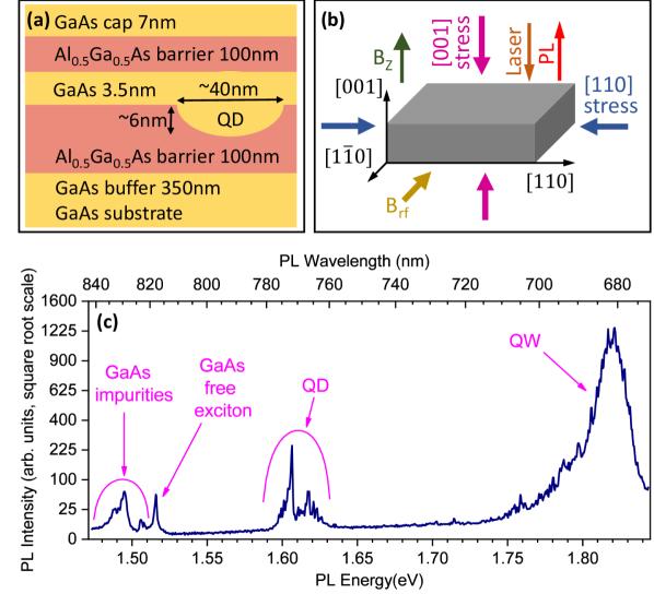
Figure 1: (a) Sample structure showing the sequence of GaAs and Al_0.5Ga_0.5As epitaxial layers. (b) Schematic of the experiment geometry showing orientation of a sample, direction of the static magnetic field $B_{z}$, radio frequency field $B_{rf}$, and the direction of the photoluminescence excitation and collection. External stress is applied either along the $[001]$ direction or the $[110]$ direction. (c) Typical photoluminescence spectrum at $B_{z}=0$ showing emission from the quantum well (QW), a single quantum dot (QD), as well as emission from the GaAs substrate which includes free exciton emission and impurity-induced recombination. Square-root vertical scale is used to reveal weak spectral features.

The structure was cleaved into small parallelepiped pieces with dimensions of $\sim 0.9\times 1.5\times 0.35$ mm along the $[110]$, $[1\bar{1}0]$ and $[001]$ directions respectively. Three samples were prepared. The first sample was as grown (unstressed). The second sample was glued between two flat titanium surfaces and stressed compressively along the $[110]$ direction using titanium screw and nut that press the two titanium surfaces towards each other. The third sample was glued between the bottom titanium flat surface and the top sapphire flat surface to be stressed compressively along the $[001]$ growth direction. All of the samples were studied in a configuration shown in Fig. 1(b). Magnetic field up to 10 T was aligned along the $z$-axis ($[001]$) within $\pm 2^{\circ}$, which is also the direction of the laser excitation and photoluminescence (PL) collection. For the sample stressed along the $[001]$ direction, optical excitation and PL propogated through the sapphire glass.

All experiments are conducted in a helium bath cryostat at a sample temperature $\sim$4.2 K. A small copper coil is mounted close to the sample and is used to generate radiofrequency magnetic field $B_{rf}$ along the $[1\bar{1}0]$ direction in the NMR experiments. Quantum dot NMR spectra are measured using optical hyperpolarization of the nuclear spins (via circularly polarized laser excitation) and optical detection of the electron hyperfine shifts. The signals of the quadrupolar nuclei are enhanced using ”inverse” NMR technique Chekhovich et al. (2012). A detailed description and analysis of the relevant NMR methods has been reported previously Chekhovich et al. (2012), and is not repeated here: in this work we use these techniques as a tool that gives an accurate spectral distribution of the resonant frequencies of the nuclei within the volume of an individual quantum dot. The excitation laser is focused into a spot of $\sim$1 $\mu$m in diameter, so that carriers are generated simultaneously in the QW, the GaAs buffer layer, and the QDs within the area of the laser spot. The photoluminescence signal is collected and analyzed with a grating spectrometer and a charge coupled device (CCD) camera.

A typical broadband PL spectrum measured under HeNe laser excitation ($632.8$ nm) is shown in Fig. 1(c). Spectral features observed include emission from the QW ($\sim$1.85 eV), free exciton emission of the bulk GaAs buffer and substrate layers ($\sim$1.515 eV), impurity-induced PL of bulk GaAs ($\sim$1.48-1.51 eV) including bound excitons as well as recombination involving donor and acceptor states Gurioli et al. (1998); Shah et al. (1969); Kudo et al. (1986); Gopal et al. (2000); Amo et al. (2006); Sell et al. (1973). Quantum dot emission is observed at $\sim$1.60-1.63 eV and consists of several narrow spectral lines corresponding to different exciton states of a single QD. Since photoluminescence is excited only in a small area of the sample, the spectrum of GaAs free exciton can be used to probe local strain fields in a $\sim$1 $\mu$m sized spot. Moreover, NMR is detected from the spectral shifts in the QD emission and thus samples an even smaller nanometer-sized part of the optically excited area. In this way it is ensured that GaAs PL spectroscopy and QD NMR sample the same strain field.

IV Experimental results and analysis

IV.1 Effect of strain on GaAs photoluminescence and nuclear magnetic resonance spectra

Figure 2(a) shows GaAs free exciton PL spectra measured in three different samples at $B_{z}$=0, while Fig. 2(b) shows ⁷⁵As NMR spectra measured at $B_{z}$=8 T from the QDs in the same optically excited spots as in (a). Since the size of the optically excited spot is much smaller than the size of the sample, and the stiffness tensors of GaAs and AlAs are very similar Vurgaftman et al. (2001) all significant variations of strain induced by external stress occur on length scales that are much larger than the studied spot size. As a result the two types of spectroscopy probe the same strain field.

Bulk GaAs PL is measured with laser excitation intensity $\sim$5$\times 10^{6}$ W/m². On the one hand it is high enough to saturate the impurity-induced PL and make free exciton emission dominant, while on the other hand it is low enough to avoid excessive spectral broadening. In an unstressed sample PL is detected with a variable orientation of linear polarization: the top two spectra in Fig. 2(a) are measured along the orthogonal polarization axes and reveal very small polarization degree and a negligible splitting. This is expected for unstrained GaAs PL, since the valence band state at $k=0$ is four-fold degenerate. The corresponding NMR spectrum (Fig. 2(b), top) reveals a triplet of lines with a small quadrupolar splitting $|\nu_{Q}|\approx$26.2 kHz, most likely related to the strain arising from the residual lattice mismatch of the GaAs and Al_0.5Ga_0.5As layers. Each line of the triplet corresponds to an individual dipolar nuclear spin transition $I_{z}\leftrightarrow I_{z+1}$ as labeled in Fig. 2(b).

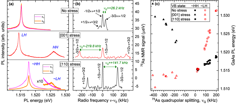
Figure 2: Effect of strain on bulk GaAs photoluminescence (PL) and quantum dot NMR spectra. (a) Free-exciton PL from a GaAs substrate measured at $B=$0 T under excitation with a photon energy $\sim$1.54 eV and intensity $\sim$5$\times 10^{6}$ W/m² in an unstressed sample (top), sample stressed along $[001]$ (middle), and sample stressed along $[110]$ (bottom). In an unstressed sample emission has negligible splitting between peaks detected in two orthogonal linear polarizations ($\pi_{1}$, $\pi_{2}$). Stress along $[001]$ splits luminescence spectrum into two non-polarized peaks corresponding to emission of light (LH) and heavy (HH) hole excitons. Stress along $[110]$ splits luminescence spectrum into a stronger peak with partial linear polarization corresponding to emission from a predominantly HH exciton, and a weak linearly polarized peak from a predominantly LH exciton (parts of the spectra with $\times 10$ vertical magnification are shown to reveal the $\sim$LH peak). (b) Nuclear magnetic resonance spectra of ⁷⁵As nuclei measured with $\sigma^{+}$ polarized optical excitation at $B_{z}=$8 T ($\nu_{0}\approx$58.46 MHz) on GaAs/AlGaAs quantum dots from the same spots as GaAs luminescence spectra in (a). Well-resolved NMR triplets arising from quadrupolar effects are observed. In an unstressed sample small quadrupolar shift $\nu_{Q}$ is observed due to the residual strain of the GaAs/AlGaAs heterostructure. Under $[001]$ ($[110]$) stress, the resulting strain shifts the $-3/2\leftrightarrow-1/2$ satellite transition to lower (higher) frequency corresponding to negative (positive) $\nu_{Q}$. (c) Energies of predominantly HH (solid symbols) and LH (open symbols) bulk GaAs PL peaks plotted against quadrupolar shift $\nu_{Q}$ measured in multiple quantum dots in an unstressed (circles), $[001]$-stressed (triangles), and $[110]$-stressed (squares) samples. GaAs PL energies and NMR frequencies are derived from the spectra using Lorentzian and Gaussian peak fitting respectively. Variation of $\nu_{Q}$ and PL energies in each sample is due to the inhomogeneity of strain across the sample surface – the exception is the four points at $\nu_{Q}\approx+200$ kHz that were measured at an increased stress along $[110]$.

For the sample stressed along $[001]$, GaAs free exciton PL is split into two non-polarized lines (Fig. 2(a), middle). This is expected, since deformation along $[001]$ lifts the degeneracy and splits the state at the top of the valence band into a two-fold degenerate state with momentum projection $j=\pm 1/2$ corresponding to the light holes (LH), and a two-fold degenerate state with $j=\pm 3/2$ corresponding to the heavy holes (HH). The effect of strain is also manifested in NMR through a significantly larger triplet splitting $|\nu_{Q}|\approx$219.8 kHz (Fig. 2(b), middle).

The stress along $[110]$ also splits the four-fold degenerate top of the valence band into two doublets. These however are no longer pure heavy and light hole states, and their recombination results in a linearly polarized PL (Fig. 2(a), bottom). The peak at $\sim$1.518 eV is partially linearly polarized and corresponds to the state with predominantly heavy hole character ($\sim$HH). By contrast, the peak at $\sim$1.525 eV is strongly polarized and corresponds to a predominantly light hole state ($\sim$LH). The intensity of the $\sim$LH peak is reduced due to the relaxation into the $\sim$HH state. The NMR triplet splitting (Fig. 2(b), bottom) is also significantly larger than in an unstressed sample with $|\nu_{Q}|\approx$141.7 kHz.

The measurements of GaAs free exciton PL and ⁷⁵As NMR were repeated on multiple spots in all three samples and spectra similar to those shown in Fig. 2(a,b) were observed. For each spot PL energies and NMR frequencies were derived by fitting the spectral peaks. The resulting summary in Fig. 2(c) shows PL energies of $\sim$HH/HH (solid symbols) and $\sim$LH/LH (open symbols) excitons as a function of the quadrupolar splitting $\nu_{Q}$ in an unstressed (circles), $[001]$-stressed (triangles), and $[110]$-stressed (squares) samples. It can be seen that in the unstressed sample $\nu_{Q}$ varies in a small range between 15 and 30 kHz, due to the differences in the residual strains in the individual quantum dots, while GaAs PL peak energy varies in a small range between 1.5145 and 1.5155 eV, most likely due to the local residual strains arising from crystal imperfections. The spectral shifts in the stressed samples are significantly larger than the random variations in the unstressed sample. There is a clear trend in Fig. 2(c) that larger quadrupolar shifts are correlated with larger GaAs PL energy shifts. On the other hand, the stress-induced spectral shifts (both in PL and NMR) vary across the surface area of the sample, since non-uniform contact between the sample and the titanium stress mount leads to spatial non-uniformity of the stress and strain fields. However, these non-uniformities have characteristic lengths much larger than the laser excitation spot, so that the strain detected in optical PL and NMR spectra can be treated as constant for each individual spot.

For the purpose of quantitative analysis it is convenient to re-plot the data of Fig. 2(c) in a different form. This is shown in Fig. 3 where the average energy of LH and HH (solid symbols, left scales) as well as the splitting of the LH and HH (open symbols, right scales) are plotted as a function of $\nu_{Q}$ for the $[001]$-stressed (a) and $[110]$-stressed (b) samples.

In case of the $[001]$-stressed sample [Fig. 3(a)], the average energy of LH and HH shows significant random variations. By contrast, the LH-HH splitting is very well described by a linear dependence on $\nu_{Q}$. The best fit is shown by a dashed line in Fig. 3(a) and the slope is $k_{[001]}^{-}=46.5\pm 0.8\mu$eV/kHz (95% confidence interval). The situation is reversed for the sample stressed along $[110]$ as shown in Fig. 3(b). While the LH-HH splitting shows variations, the dependence of the average LH and HH recombination energies is well described by a linear function (solid line) with a fitted slope $k_{[110]}^{+}=55.1\pm 1.5\mu$eV/kHz. As we show below, such a difference between the cases of $[001]$-stressed and $[110]$-stressed samples is not a coincidence. With some basic assumptions about the spatial distribution of strain in the stressed samples the measured $k_{[001]}^{-}$ and $k_{[110]}^{+}$ values are used to derive the gradient elastic tensor component $S_{11}$ as show in Sec. IV.4. Prior to this derivation, in the next subsections we present analysis of the properties of the gradient-elastic tensor that require no assumptions about strain configuration.

It is worth noting that rigorous analysis of bulk GaAs PL spectra requires taking into account electron-hole exchange interaction and polariton effects. However, these effects are of the order of $\sim$0.25 meV, which is significantly smaller than the strain induced spectral shifts observed here. More importantly, it has been shown that the strain-induced spectral shifts of all the PL components are well described by the free electron and hole deformation potentials Sell et al. (1973). Since our subsequent analysis relies only on the ratios of the strain-induced PL and NMR spectral shifts (rather than absolute GaAs PL energies), it is sufficient to use a simplified ”free-exciton” description of the GaAs PL ignoring polariton effects.

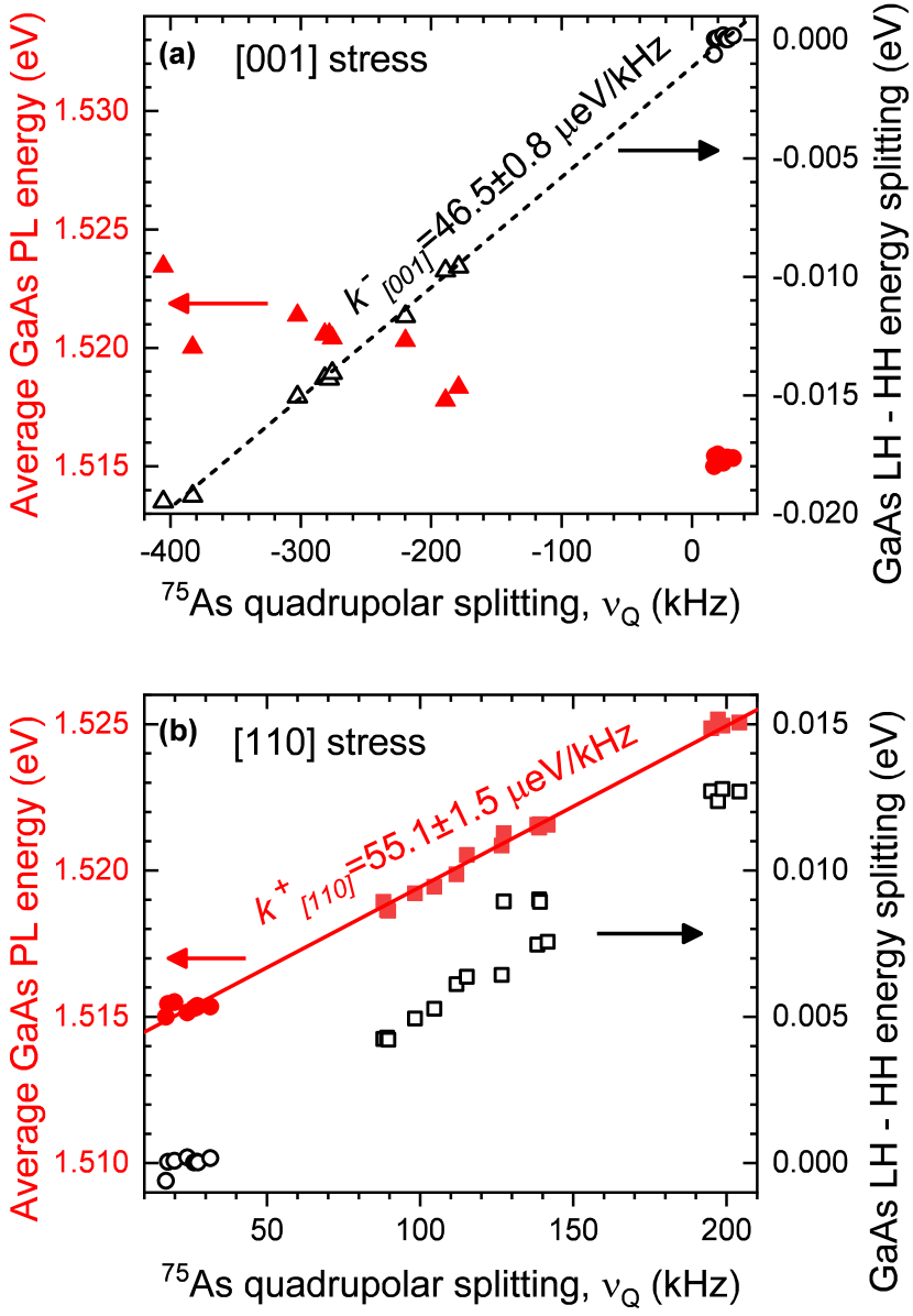
Figure 3: Data of Fig. 2(c) plotted in terms of the arithmetic average PL energy of the LH and HH excitons (solid symbols, left scales) and the difference of the LH and HH exciton PL energies (open symbols, right scales) as a function of ⁷⁵As quadrupolar shift $\nu_{Q}$. (a) Results for the unstressed (circles) and $[001]$-stressed (triangles) samples. LH-HH splitting is well described by a linear function with a slope $k_{[001]}^{-}=46.5\pm 0.8~{}\mu$eV/kHz (dashed line). (b) Results for the unstressed (circles) and $[110]$-stressed (squares) samples. The average LH-HH PL energy is well described by a linear function with a slope $k_{[110]}^{+}=55.1\pm 1.5~{}\mu$eV/kHz (solid line).

IV.2 Measurement of the sign of the $S$-tensor components

We now show how the sign of the gradient-elastic tensor can be determined directly, if it is possible to identify spin projections of the nuclear spin states corresponding to each NMR transitions. The nuclear spin states can be identified from the hyperfine interaction effects, if the sing of the electron spin polarization is known. In order to define the sign of the electron spin polarization we start by considering the signs of the carrier $g$-factors. The electron $g$-factor in the studied QDs Ulhaq et al. (2016) as well as in thin GaAs/AlGaAs quantum wells Snelling et al. (1992) is small and the shifts of the excitonic levels induced by magnetic field along the growth axis are dominated by the hole Zeeman effect. The sign of the hole $g$-factor Snelling et al. (1992); Ulhaq et al. (2016) is such that at positive magnetic field $B_{z}>0$ the exciton with a positive (negative) hole momentum projection $j_{z}$=$+3/2$ ($-3/2$) labeled $\Uparrow$ ($\Downarrow$) has higher (lower) energy. In order to be optically active the high- (low-) energy exciton must have electron spin projection $s_{z}$=$-1/2$ ($+1/2$) denoted $\downarrow$ ($\uparrow$). Figure 4(a) shows PL spectra of a neutral exciton in a typical QD at $B_{z}=8$ T measured under $\sigma^{+}$ and $\sigma^{-}$ optical excitation at $\sim$1.65 eV. Each PL spectrum is a doublet of optically allowed (”bright”) excitons, with high- (low-) energy Zeeman component corresponding to recombination of a $\Uparrow\downarrow$ ($\Downarrow\uparrow$) exciton.

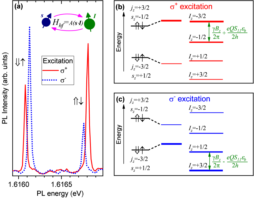
Figure 4: Derivation of the sign of the gradient elastic tensor. (a) Photoluminescence spectra of a QD neutral exciton measured at $B_{z}$=8 T under $\sigma^{+}$ (solid line) and $\sigma^{-}$ (dashed line) polarized excitation at 1.65 eV. The $\sigma^{+}$ excitation predominantly populates the exciton state with hole spin $s_{z}=+3/2$ ($\Uparrow$) and electron spin $s_{z}=-1/2$ ($\downarrow$), while $\sigma^{-}$ excitation predominantly populates the $\Downarrow\uparrow$ exciton. Electron spin $\mathbf{s}$ can be transferred to a nuclear spin $\mathbf{I}$ via hyperfine interaction (inset) resulting in dynamic nuclear polarization, which in turn leads to hyperfine shifts of the exciton transitions. (b) Schematic of spin effects under $\sigma^{+}$ excitation which increases population of the $s_{z}=-1/2$ excitons (thicker horizontal line) and reduces population of the $s_{z}=+1/2$ exciton (thinner line). Dynamic nuclear polarization enhances the population of the $I_{z}=-3/2$ nuclear spin states. This is observed as a hyperfine shift of the $s_{z}=-1/2$ excitons to higher energy and enhanced amplitude of the $-3/2\leftrightarrow-1/2$ NMR transition with frequency $\frac{\gamma B_{z}}{2\pi}+\frac{eQ}{2h}S_{11}\epsilon_{b}$. (c) Excitation with $\sigma^{-}$ light leads to the opposite sign of electron and nuclear spin polarizations, enhancing the $+1/2\leftrightarrow+3/2$ NMR transition at frequency $\frac{\gamma B_{z}}{2\pi}-\frac{eQ}{2h}S_{11}\epsilon_{b}$. By matching the signs of the exciton spectral shifts in (a) and the sign of the NMR spectral shifts [cf. Fig. 2(b)] it is possible to deduce the sign of the gradient elastic tensor component $S_{11}$ (see Sec. IV.2).

Two effects are observed under circularly polarized excitation in Fig. 4(a): (i) the emission intensity of the high-(low-) energy Zeeman component is enhanced under $\sigma^{+}$ ($\sigma^{-}$) excitation, and (ii) the Zeeman splitting increases (decreases) under $\sigma^{+}$ ($\sigma^{-}$) excitation due to the buildup of nuclear spin polarization. These two effects are related: to understand their origin we first consider the case of $\sigma^{+}$ excitation [Fig. 4(b)], which generates predominantly $\Uparrow\downarrow$ excitons. During repeated optical excitation the $s_{z}=-1/2$ electrons transfer their polarization to the nuclei of the dot via the flip-flop process Chekhovich et al. (2017) enabled by the hyperfine interaction. Since the flip-flops are spin-conserving, the nuclei become predominantly polarized into the states with negative spin $I_{z}<0$. The net nuclear spin polarization back-acts on the electron spin via hyperfine interaction, described by the Hamiltonian $\hat{H}_{hf}=A(\hat{s}\cdot\hat{I})$. The hyperfine constant $A$ is positive for Ga and As nuclei due to their positive gyromagnetic ratios $\gamma>0$. As a result the $\Uparrow\downarrow$ exciton shifts to higher energy under $\sigma^{+}$ excitation. In a similar manner, under $\sigma^{-}$ excitation [Fig. 4(c)] the population of the $\Downarrow\uparrow$ exciton is enhanced, and it also shifts to higher energy since now both $s_{z}$ and $I_{z}$ are positive. This is indeed observed in Fig. 4(a): the Zeeman component whose intensity is enhanced by circularly polarized excitation always shifts to higher energy. This observation confirms the positive sign of $A$ and that the spin flip-flops are the source of dynamic nuclear spin polarization. Taking also into account the signs of the electron and hole $g$-factors, we conclude that circularly polarized excitation that enhances the high- (low-) energy exciton population and labeled here $\sigma^{+}$($\sigma^{-}$), populates predominantly nuclear spin states with negative (positive) projection $I_{z}$.

For the NMR spectra measured with $\sigma^{+}$ optical excitation the population of the $I_{z}=-3/2$ and $I_{z}=-1/2$ states is enhanced as discussed above. As a result the amplitude of the $-3/2\leftrightarrow-1/2$ satellite NMR peak exceeds the amplitude of the $+1/2\leftrightarrow+3/2$ satellite STs . The spectra of Fig. 2(b) were measured under $\sigma^{+}$ optical excitation (i.e., excitation that enhances the intensity of the high energy Zeeman exciton component). For the case of compressive stress along $[001]$ the $-3/2\leftrightarrow-1/2$ NMR peak has a lower frequency than the $-1/2\leftrightarrow+1/2$ central peak [middle spectrum in Fig. 2(b)], corresponding to $\nu_{Q}<0$. The quadrupolar shift $\nu_{Q}$ is related to strain via Eqs. 14, 15 and we find that $\nu_{Q}=\frac{eQ}{2h}S_{11}\epsilon_{b}<0$ in this experiment. In case of $[001]$ compression $\epsilon_{b}<0$, and since the quadrupolar moment of ⁷⁵As is positiveStone (2016) $Q>0$, we concluded that $S_{11}>0$ for ⁷⁵As.

While in the above calculations we assumed $B_{z}>0$, the opposite assumption $B_{z}<0$ leads to the same conclusions about the signs of the gradient elastic tensor components $S_{11}$. Finally, we note that in previous work on InGaAs/GaAsChekhovich et al. (2012) and GaAs/AlGaAsUlhaq et al. (2016) QDs, the shift of the $-3/2\leftrightarrow-1/2$ satellite peak to lower frequency was arbitrarily assigned a positive $\nu_{Q}$ value since the sign of $S_{11}$ was undefined. By contrast, in the present work the sign of $\nu_{Q}$ is strictly determined by Eqs. 2, 14, 15 and the signs of $S_{11}$ and $Q$.

IV.3 Measurement of the ratio of the electric field gradients on $As$ and $Ga$ lattice sites

Measurement of NMR via optical detection of the hyperfine shifts in the PL spectra of a quantum dot guarantees that only the nuclei of a single quantum dot contribute to the NMR spectrum. Thus if NMR spectrum is measured on As and Ga nuclei of the same quantum dot, one can ensure that the nuclei of the two isotopes belong to the same nanoscale volume and probe the same strain field. Then, according to Eq. 2, the ratio of the quadrupolar shifts of the two isotopes is simply $\nu_{Q}^{{}^{69}\mathrm{Ga}}/\nu_{Q}^{{}^{75}\mathrm{As}}=(Q^{{}^{69}\mathrm{Ga}}S_{11}^{{}^{69}\mathrm{Ga}})/(Q^{{}^{75}\mathrm{As}}S_{11}^{{}^{75}\mathrm{As}})$ and does not depend on the actual strain magnitude $\epsilon_{b}$. Figure 5(a) shows NMR spectra of ⁶⁹Ga (top) and ⁷⁵As (bottom) measured on the same quantum dot at $B_{z}=$5.5 T using $\sigma^{+}$ optical excitation. Both isotopes have spin $I=$3/2 giving rise to the well resolved NMR triplets with different quadrupolar splittings $\nu_{Q}$. We note that the satellite peak with higher amplitude, corresponding to the $-3/2\leftrightarrow-1/2$ transition, appears on the low (high) frequency side for Ga (As) implying opposite signs of $\nu_{Q}$ and hence opposite signs of $QS_{11}$ for the two isotopes. Since $S_{11}>0$ for ⁷⁵As and $Q>0$ for all stable Ga and As isotopes we conclude that $S_{11}<0$ for ⁶⁹Ga and ⁷¹Ga. Similar measurements of ⁶⁹Ga and ⁷⁵As NMR were conducted on several quantum dots in an unstressed and stressed samples and are summarized in Fig. 5(b) where $\nu_{Q}^{{}^{69}\mathrm{Ga}}$ is shown as a function of $\nu_{Q}^{{}^{75}\mathrm{As}}$ by the symbols. The linear fit is shown by the line and yields the slope $k_{{}^{69}\mathrm{Ga}/^{75}\mathrm{As}}=(Q^{{}^{69}\mathrm{Ga}}S_{11}^{{}^{69}\mathrm{Ga}})/(Q^{{}^{75}\mathrm{As}}S_{11}^{{}^{75}\mathrm{As}})=-0.495\pm 0.012$. Taking the values of quadrupolar moments Stone (2016) $Q^{{}^{69}\mathrm{Ga}}=0.171\times 10^{-28}$ m² and $Q^{{}^{75}\mathrm{As}}=0.314\times 10^{-28}$ m² we calculate for the ratio of the components of the gradient elastic tensors: $S_{11}^{{}^{69}\mathrm{Ga}}/S_{11}^{{}^{75}\mathrm{As}}=-0.909$ so that the magnitude of the strain-induced EFG is smaller at the gallium sites.

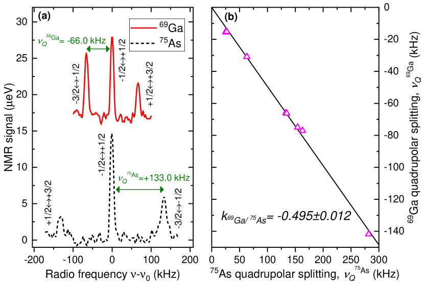
Figure 5: (a) NMR spectra of a single quantum dot measured at high magnetic field $B_{z}\approx 5.5$ T on ⁷⁵As nuclei ($\nu_{0}\approx$40.27 MHz, dashed line) and ⁶⁹Ga nuclei ($\nu_{0}\approx$56.46 MHz, solid line). Both isotopes are spin-3/2 and exhibit well resolved quadrupolar triplets with different splittings $\nu_{Q}$. (b) Dependence of the ⁶⁹Ga quadrupolar splitting $\nu_{Q}^{{}^{69}\mathrm{Ga}}$ on the ⁷⁵As splitting $\nu_{Q}^{{}^{75}\mathrm{As}}$ measured on different individual quantum dots in an unstressed sample as well as in samples stressed along $[001]$ or $[110]$ crystal axes (symbols). Linear fitting is shown by the solid line and its slope $k_{{}^{69}\mathrm{Ga}/^{75}\mathrm{As}}=-0.495\pm 0.012$ gives an estimate of the ratio $(Q^{{}^{69}\mathrm{Ga}}S_{11}^{{}^{69}\mathrm{Ga}})/(Q^{{}^{75}\mathrm{As}}S_{11}^{{}^{75}\mathrm{As}})$ between the products of gradient elastic tensor components $S_{11}$ and quadrupolar moments $Q$ of ⁶⁹Ga and ⁷⁵As in GaAs.

IV.4 Derivation of the gradient-elastic tensor component $S_{11}$ in GaAs

We now discuss how simultaneous measurements of GaAs free exciton PL and QD NMR presented in Section IV.1 can be used to calibrate the fundamental material parameters of GaAs. First we consider the case of a sample stressed along the $[001]$ direction. If the stress is produced by applying a uniform $z$-oriented pressure to the top and bottom $(001)$ surfaces of the sample, the resulting strain has a very simple configuration where $\epsilon_{h}$ and $\epsilon_{b}$ are finite, while $\epsilon_{\eta}$ and $\epsilon_{s}$ vanish for symmetry reasons ($\epsilon_{xx}=\epsilon_{yy}$ and $\epsilon_{xy}=\epsilon_{yz}=\epsilon_{zx}=0$). In this case according to Eq. 1 the splitting between the LH and HH PL transition energies is simply $2|b\epsilon_{b}|$. Since both the LH-HH exciton splitting and the NMR shift now depend only on $\epsilon_{b}$, their ratio can be taken to eliminate $\epsilon_{b}$ and we find:

$$\begin{split}k_{[001]}^{-}=-\frac{4hb}{eQS_{11}},\end{split}$$ (3)

where the minus sign is added to account for the fact that the PL of the predominantly LH exciton has a lower energy at $\epsilon_{b}<0$. The $k_{[001]}^{-}$ has been measured experimentally for ⁷⁵As (see Fig. 3(a) and Section IV.1).

In a real sample, the pressure on the surfaces of the sample is not necessarily uniform and aligned to the $z$ axis. In this case Eq. 3 holds only at the geometrical centre of the top $(001)$ surface (for symmetry reasons), while away from the centre the non-diagonal strain components may arise leading e.g. to $\epsilon_{s}\neq 0$. According to Eqs. 1, 2 the effect of the finite $\epsilon_{s}$ or $\epsilon_{\eta}$ is to induce an additional splitting of the heavy and light hole excitons without affecting the NMR spectral splitting $\nu_{Q}$, in which case the dependence of the LH-HH splitting on $\nu_{Q}$ would no longer be linear when measured over the surface of the sample. In experiment, multiple spots of the $[001]$-stressed sample, both at the centre of the sample surface and close to the edges were investigated. The strain can be seen to vary significantly across the sample surface: $\nu_{Q}$ is found to range between $-$400..$-$180 kHz [Fig. 3(a)] indicating variation of $\epsilon_{b}$, while the spread in the average GaAs PL energies [full triangles in Fig. 3(a)] indicates variation of $\epsilon_{h}$. On the other hand the resulting dependence of the LH-HH splitting on $\nu_{Q}$ is still well described by a linear function [open triangles and dashed line in Fig. 3(a)]. This can only be if $\epsilon_{s}$ and $\epsilon_{\eta}$ are small in the studied sample and thus the experimentally measured ratio $k_{[001]}^{-}=46.5\pm 0.8\mu$eV/kHz describes the relation of the fundamental parameters $b$ and $S_{11}$ of GaAs according to Eq. 3.

We now consider the case of a sample stressed along the $[110]$ direction. If the stress is produced by applying a uniform pressure along $[110]$ to the $(110)$ surfaces of the sample the resulting strain will have non-zero $\epsilon_{h}$, $\epsilon_{b}$, as well as $\epsilon_{s}$ arising from the $\epsilon_{xy}$ component. (Recall that $x$ and $y$ axes are aligned along $[100]$ and $[010]$ respectively, so that $\epsilon_{xy}=\epsilon_{xx}=\epsilon_{yy}$ under uniform stress along $[110]$). Even in an ideal case the GaAs PL energies (Eq. 1) under $[110]$ stress involve the $d^{2}\epsilon_{s}^{2}$ term, making it difficult to relate to the NMR shifts given by Eq. 2. In a real sample, the non-diagonal shear strain $\epsilon_{xy}$ is not necessarily constant and $\epsilon_{\eta}$ is not necessarily zero due to the inevitable non-uniformities of the stress induced by the titanium strain mount. This is evidenced in Fig. 3(b) where the LH-HH splitting (open squares) is seen to deviate considerably from a linear dependence on $\nu_{Q}$, which is proportional only to $\epsilon_{b}$.

However, it is possible to eliminate the effect of the unknown shear strain components $\epsilon_{s}$, $\epsilon_{\eta}$ in a $[110]$-stress configuration. For that we notice that the top $(001)$ surface of the sample which is studied optically is free from external stress (traction free). As a result, the boundary conditions dictateBarber (2010) that three of the components of the mechanical stress tensor vanish $\sigma_{zx}=\sigma_{zy}=\sigma_{zz}=0$, and the only non-zero components are $\sigma_{xx}$, $\sigma_{yy}$, $\sigma_{xy}$. Writing down the strain-stress relation one can easily verify that in a GaAs crystal (cubic symmetry), the ratio of the biaxial and hydrostatic strains at the free $(001)$ surface does not depend on the actual $\sigma_{xx}$, $\sigma_{yy}$, $\sigma_{xy}$ values and equals $\epsilon_{b}/\epsilon_{h}=\frac{\sigma_{xx}+\sigma_{yy}}{2c_{12}+c_{11}}/\frac{\sigma_{xx}+\sigma_{yy}}{2c_{12}-2c_{11}}=\frac{2c_{12}+c_{11}}{2c_{12}-2c_{11}}\approx-1.742$, where $c_{11}$ and $c_{12}$ are the stiffness constants of GaAsAdachi (2009). Now we use this relation to express $\epsilon_{b}$ through $\epsilon_{h}$ in Eq. 2 to make quadrupolar shift $\nu_{Q}$ depend only on $\epsilon_{h}$. Since the average LH-HH shift of the GaAs PL energy $a\epsilon_{h}$ also depends only on $\epsilon_{h}$ (Eq. 1) it can be related to $\nu_{Q}$ by eliminating the strain to find:

$$\begin{split}k_{[110]}^{+}=\frac{4ha}{eQS_{11}}\frac{c_{12}-c_{11}}{2c_{12}+c_{11}},\end{split}$$ (4)

The solid symbols and the line in Fig. 3(b) demonstrate that the average GaAs PL energy is indeed a linear function of $\nu_{Q}$, confirming the invariance of $\epsilon_{b}/\epsilon_{h}$ at the surface of the studied sample. Thus Eq. 4 relates the $a$ and $S_{11}$ parameters through the experimentally measured value $k_{[110]}^{+}=55.1\pm 1.5~{}\mu$eV/kHz.

Table 1: GaAs parameters.

Parameter	Units	Previous work	This work
$a=a_{c}+a_{v}$	eV	$-8.7$ Pollak et al. (1966); $-8.9$ Bhargava and Nathan (1967); $-8.7$ Bendorius and Shileika (1970); $-8.93$ Chandrasekhar and Pollak (1977); $-8.72$ Qiang et al. (1990); $-10.19$ Mair et al. (1998); $-8.5$ Vurgaftman et al. (2001); $-8.8$ Adachi (2009)
$b$	eV	$-2.1$ Pollak et al. (1966); $-1.96$ Bhargava and Nathan (1967); $-1.76$ Chandrasekhar and Pollak (1977); $-2.00$ Qiang et al. (1990); $-2.00$ Mair et al. (1998); $-2.0$ Vurgaftman et al. (2001); $-1.85$ Adachi (2009)
$b/a$		$0.24$ Pollak et al. (1966); $0.22$ Bhargava and Nathan (1967); $0.20$ Chandrasekhar and Pollak (1977); $0.23$ Qiang et al. (1990); $0.20$ Mair et al. (1998); $0.24$ Vurgaftman et al. (2001); $0.21$ Adachi (2009)	${0.241\pm 0.008}$
$c_{11}$	GPa	$122.1$ Vurgaftman et al. (2001); $118.8$ Adachi (2009)
$c_{12}$	GPa	$56.6$ Vurgaftman et al. (2001); $53.8$ Adachi (2009)
$c_{44}$	GPa	$60.0$ Vurgaftman et al. (2001); $59.4$ Adachi (2009)
$\frac{2c_{12}+c_{11}}{2c_{12}-2c_{11}}$		$-1.796$ Vurgaftman et al. (2001); $-1.742$ Adachi (2009)
$\frac{Q^{{}^{69}\mathrm{Ga}}S_{11}^{{}^{69}\mathrm{Ga}}}{Q^{{}^{75}\mathrm{As}}S_{11}^{{}^{75}\mathrm{As}}}$		$-0.508$ Sundfors (1974)	${-0.495\pm 0.012}$
$Q^{{}^{75}\mathrm{As}}S_{11}^{{}^{75}\mathrm{As}}$	$10^{-6}$ V	$\pm 1.06$ Sundfors (1974)	${+0.76}$
$Q^{{}^{69}\mathrm{Ga}}S_{11}^{{}^{69}\mathrm{Ga}}$	$10^{-6}$ V	$\mp 0.543$ Sundfors (1974)	${-0.37}$
$Q^{{}^{69}\mathrm{Ga}}$	$10^{-28}$ m2	$0.171$ Stone (2016)
$Q^{{}^{75}\mathrm{As}}$	$10^{-28}$ m2	$0.314$ Stone (2016)
$S_{11}^{{}^{75}\mathrm{As}}$	$10^{21}$ V/m2	$\pm 34.0$ Sundfors (1974)	${+24.1}$
$S_{11}^{{}^{69}\mathrm{Ga}}$	$10^{21}$ V/m2	$\mp 31.7$ Sundfors (1974)	${-21.9}$

Since the absolute values of stress and strain are not measured in our experiment, the results presented above can be used to estimate the ratios of the GaAs parameters. The absolute value of a parameter can then be estimated by taking the values of other parameters from the previous studies.

The elementary charge $e$ and the Planck constant $h$ are known with very high accuracy. The stiffness constants of GaAs $c_{11}$ and $c_{12}$ are also known with a good accuracy. While $c_{11}$ and $c_{12}$ in GaAs exhibit some temperature dependence, the ratio $c_{11}/c_{12}$ used in our analysis is reported to be nearly invariant from cryogenic to room temperature Cottam and Saunders (1973). Here we use the $c_{11}$, $c_{12}$ values at 300 K from Ref. Adachi (2009). This leaves three GaAs parameters: the deformation potentials $a=(a_{c}+a_{v})$, $b$ and the $QS_{11}$ product of ⁷⁵As. Since there are two experimentally measured ratios (Eqs. 3, 4), these three parameters can be linked by two independent relations.

One of the relations can be obtained by dividing Eqs. 3 and 4 to eliminate $QS_{11}$ which gives the ratio of the deformation potentials:

$$\begin{split}&\frac{b}{a}=\frac{k_{[100]}^{-}}{k_{[110]}^{+}}\frac{c_{12}-c_{11}}{2c_{12}+c_{11}}=\\ &\quad\quad=(0.841\pm 0.027)\frac{c_{12}-c_{11}}{2c_{12}+c_{11}}=0.241\pm 0.008,\end{split}$$ (5)

where the error estimate is purely due to the experimental uncertainty in $k_{[100]}^{-}$ and $k_{[110]}^{+}$ and there can be an additional error due to the $\sim\pm$2% uncertainty in the $c_{11}$, $c_{12}$ values. Our estimate of $b/a$ is in excellent agreement with the ratio derived from the recommended Vurgaftman et al. (2001); Adachi (2009) values of $a$ and $b$ based on a number of independent experimental and theoretical studies. Such agreement supports the validity of our experimental method based on relating PL and NMR spectral shifts. The estimates derived in this work are summarized in Table 1 together with the results of the earlier work.

For the second relation we use Eq. 4 to link the deformation potential $a$ with the component of the gradient elastic tensor $S_{11}$. The variation of the GaAs fundamental gap under hydrostatic strain characterized by $a=a_{c}+a_{v}$ has been studied experimentally by several authorsDing et al. (2010); Seravalli et al. (2003); Seidl et al. (2006); Trotta et al. (2012); Rastelli et al. . There is some variation, but most experiments as well as calculations Van de Walle (1989) are consistent and it is commonly acceptedVurgaftman et al. (2001); Adachi (2009) that $a\approx-8.8$ eV. By contrast there are only few reports on experimental gradient-elastic tensors in GaAs Sundfors (1974); Bogdanov and Lemanov (1968); Guerrier and Harley (1997) with only one series of experiments where $S_{11}$ and $S_{44}$ were measured directly Sundfors (1969, 1974). Thus we use $a\approx-8.8$ eV (Ref.Adachi (2009)) to evaluate $Q^{{}^{75}\mathrm{As}}S_{11}^{{}^{75}\mathrm{As}}\approx+0.76$ $\mu$V. The uncertainty of this estimate arising from the experimental uncertainty in $k_{[110]}^{+}$ is only $\pm 3\%$, so the main error is likely to arise from the uncertainty in $a$, which is approximately $\pm 5\%$ based on the spread of the values derived in different independent studies. Using the $k_{{}^{69}\mathrm{Ga}/^{75}\mathrm{As}}$ ratio measured in Sec. IV.3 we also estimate $Q^{{}^{69}\mathrm{Ga}}S_{11}^{{}^{69}\mathrm{Ga}}\approx-0.37$ $\mu$V for ⁶⁹Ga with a similar relative uncertainty. These values are $\sim$30% smaller than those derived by SundforsSundfors (1974) from the nuclear acoustic resonance measurements (Table 1). We point out here that normally it is the $QS_{11}$ product and not $S_{11}$ that is measured in NMR experiments and is used to predict the NMR spectra in strained semiconductor structures – the individual values for $S_{ijkl}$ and $Q$ are not accessible in conventional NMR measurements. Nonetheless, for the reference, we quote in Table 1 the $S_{11}$ values derived in this work and reported in Ref.Sundfors (1974), where in both case we divided the measured $QS_{11}$ products by the most recent recommended valuesStone (2016) of quadrupolar moments $Q$. For practical applications, it is preferable to use the $QS_{11}$ product values, or when using $S_{ijkl}$ and $Q$ separately, take their values from the same source. We also note that the $S_{11}$ values in Ref.Sundfors (1974) are in the c.g.s. units of $\times 10^{15}$ statcoulomb/cm³ and are multiplied here by 2997924.580 to convert them to the V/m² SI units.

V Discussion and conclusion

An important feature of this work is that elastic strain is probed optically through the spectral shifts the free exciton PL in bulk GaAs. This method offers certain advantages: there is no need to measure the stress or control precisely the size and the shape of the sample, moreover the strain can be probed locally on a micrometer scale, so that modest strain inhomogeneities across the sample are not a limitation. The downside is that the accuracy of the measured strain is limited by the current uncertainty in the deformation potentials. On the other hand, the detection of the nuclear quadrupolar effects in this work is achieved in a most straightforward way – by measuring the quadrupolar splitting of the NMR spectral triplet. This is different from the previous studies on GaAs Sundfors (1969, 1974) where detection was rather indirect and relied on measuring the changes of the quality factors of mechanical resonances.

The $\sim 30$% difference in the measured $S_{11}$ values between this work and the work of Sundfors Sundfors (1969, 1974) appears to be too large to be attributed to the uncertainty in deformation potentials of GaAs. On the other hand we note that the ratio of $S_{11}$ for Ga and As is in remarkably good agreement. Moreover, it was pointed out by Sundfors Sundfors (1969) that his room temperature acoustic resonance measurements of $S_{11}$ for ¹¹⁵In in InSb were notably larger than the corresponding $S_{11}$ values obtained in two independent studies using static strain Shulman et al. (1957); Bogdanov and Lemanov (1968) at 77 K. One possibility, is that all of the $S_{ijkl}$ values reported in Refs.Sundfors (1969, 1974) had a systematic offset arising from a number of parameters that needed to be calibrated for acoustic resonance measurements. Moreover, the deviation in the results may arise from the fundamental differences in how nuclear spin system responds to static and dynamic (acoustic wave) strain, as well as from the temperature dependence – these aspects remain unexplored and would require further work.

The PL/NMR method for derivation of the gradient-elastic tensor reported here have potential to be extended further. For example the $S_{44}$ component of GaAs that was not probed here, can be measured. Such a measurement would require shear strain and magnetic field which is not parallel to one of the cubic axes (e.g. $[001]$). The GaAs/AlGaAs pair is unique since it permits nearly lattice matched epitaxial growth. As a result external stress can induce deformations significantly exceeding the built-in strain, making it possible to use bandgap shifts to gauge the strain. Application to other materials, e.g. InAs/GaAs quantum wells and dots may require alternative methods for probing the strain, such as X-ray diffraction.

For practical applications the $QS_{11}$ for GaAs can be taken directly from the values measured here (Table 1). For the $QS_{44}$ parameters that were not measured here, we recommend taking the values from Ref.Sundfors (1974) and rescaling by a factor of $0.7$, which is the ratio of the $QS_{11}$ values measured here and in Ref.Sundfors (1974). Since GaAs and InAs were found to have very similar gradient elastic tensorsSundfors (1974), similar scaling by a factor of $0.7$ can be applied to the $S$-tensor values for InAs.

Appendix A Relation between strain and nuclear quadrupolar effects

The second spatial derivatives of the electrostatic potential $V(x,y,z)$ at the nuclear sites form a second rank symmetric tensor $V_{\alpha\beta}=\frac{\partial^{2}V}{\partial\alpha\partial\beta}$ ($\alpha,\beta=x,y,z$). Small deformation of a solid body is described via the second rank elastic strain tensor

$$\begin{split}\epsilon_{ij}=\frac{\partial u_{i}}{\partial x_{j}}\quad(i,j=x,y,z),\end{split}$$ (6)

where $u_{i}$ are the components of the vector field of displacements $\vec{u}(x,y,z)$ characterizing the deformation. In the limit of small deformation $V_{ij}$ is related to $\epsilon_{kl}$ via:

$$\begin{split}V_{ij}=\sum_{k,l}S_{ijkl}\epsilon_{kl}\quad(i,j,k,l=x,y,z),\end{split}$$ (7)

where $S_{ijkl}$ is a fourth rank ”gradient-elastic” tensor. Not all of its 81 components are independent, and the number of independent parameters is greatly reduced further in crystal structures with high symmetry. In case of a zinc-blend crystal (cubic symmetry group $T_{d}$) the non-vanishing elements of $S_{ijkl}$ are Shulman et al. (1957):

$$\begin{split}&S_{xxxx}=S_{yyyy}=S_{zzzz}\\ &S_{yzyz}=S_{zxzx}=S_{xyxy}\\ &S_{xxyy}=S_{yyzz}=S_{zzxx}=S_{xxzz}=S_{zzyy}=S_{yyxx}\\ \end{split}$$ (8)

Moreover, since $V_{ij}$ and $\epsilon_{ij}$ are both symmetric, the gradient elastic tensor has an additional symmetry with respect to the pari of the first and second indices as well as the pair of the third and fourth indices ($S_{ijkl}=S_{jikl}=S_{ijlk}=S_{jilk}$). Thus in a coordinate frame aligned with the crystal axes $x\parallel[100]$, $y\parallel[010]$, $z\parallel[001]$ there are in total 21 non-zero components and the tensor is fully characterized by 3 independent parameters $S_{xxxx}$, $S_{xxyy}$ and $S_{yzyz}$. Taking into account the symmetries of $S_{ijkl}$ we can evaluate Eq. 7 to find the explicit expression for the electric field gradients:

$$\begin{split}&V_{1}=V_{xx}=S_{xxxx}\epsilon_{xx}+S_{xxyy}(\epsilon_{yy}+\epsilon_{zz})=\\ &\quad=S_{xxxx}(\epsilon_{xx}-(\epsilon_{yy}+\epsilon_{zz})/2)\\ &V_{2}=V_{yy}=S_{xxxx}\epsilon_{yy}+S_{xxyy}(\epsilon_{xx}+\epsilon_{zz})=\\ &\quad=S_{xxxx}(\epsilon_{yy}-(\epsilon_{xx}+\epsilon_{zz})/2)\\ &V_{3}=V_{zz}=S_{xxxx}\epsilon_{zz}+S_{xxyy}(\epsilon_{xx}+\epsilon_{yy})=\\ &\quad=S_{xxxx}(\epsilon_{zz}-(\epsilon_{xx}+\epsilon_{yy})/2)\\ &V_{4}=V_{yz}=V_{zy}=2S_{yzyz}\epsilon_{yz}\\ &V_{5}=V_{xz}=V_{zx}=2S_{yzyz}\epsilon_{xz}\\ &V_{6}=V_{xy}=V_{yx}=2S_{yzyz}\epsilon_{xy}\end{split}$$ (9)

where the right hand side parts of the first three equations were obtained by setting $S_{xxyy}=-S_{xxxx}/2$, which is a common convention to take into account the fact that only the traceless part of $V_{ij}$ is observable in NMR Harrison and Sagalyn (1962). We have also introduced EFG components $V_{m}\quad(m=1..6)$ in Voigt notation, using which we can rewrite Eq. 9 as:

$$\begin{split}&V_{1}=S_{11}(\epsilon_{1}-(\epsilon_{2}+\epsilon_{3})/2)\\ &V_{2}=S_{11}(\epsilon_{2}-(\epsilon_{1}+\epsilon_{3})/2)\\ &V_{3}=S_{11}(\epsilon_{3}-(\epsilon_{1}+\epsilon_{2})/2)\\ &V_{4}=S_{44}\epsilon_{4}\\ &V_{5}=S_{44}\epsilon_{5}\\ &V_{6}=S_{44}\epsilon_{6},\end{split}$$ (10)

where $S_{11}=S_{xxxx}$ and $S_{44}=S_{yzyz}$. While Voigt notation simplifies the equations and is commonly accepted it needs to be used with care. Unlike $S_{ijkl}$, the 2$\times$2 matrix $S_{mn}$ is not a tensor and does not follow the tensor transformation rules. One of the consequences of this is that the definition of the non-diagonal components of strain should include an additional factor of $2$, so that $\epsilon_{4}=2\epsilon_{yz}$, $\epsilon_{5}=2\epsilon_{xz}$, $\epsilon_{6}=2\epsilon_{xy}$, while this factor of 2 is not needed in the definition of $V_{4}$, $V_{5}$, $V_{6}$ (see Eq. 9). A similar situation is encountered in the strain-stress relation $\sigma_{ij}=c_{ijkl}\epsilon_{kl}$ expressed in Voigt notation where the shear strains $\epsilon_{4}$, $\epsilon_{5}$, $\epsilon_{6}$ require a factor of 2 in their definition, while there is no such factor for the stress components $\sigma_{4}$, $\sigma_{5}$, $\sigma_{6}$ (see Ch. 10 in Ref. Newnham (2005)).

The Hamiltonian $\hat{H}_{Q}$ describing the interaction of the nucleus with spin $I$ and quadrupolar moment Q with the electric field gradients isSlichter (1990):

$$\begin{split}\hat{H}_{Q}=\frac{eQ}{6I(2I-1)h}\sum_{i,j=x,y,z}V_{ij}\left(\frac{3}{2}(\hat{I}_{i}\hat{I}_{j}+\hat{I}_{j}\hat{I}_{i})-\delta_{ij}I^{2}\right),\end{split}$$ (11)

where $e>0$ is the elementary charge, $h$ is the Planck constant, $\delta_{ij}$ is Kronecker’s delta, $\hat{I_{i}}$ are spin operator components in Cartesian coordinates and the Hamiltonian is in frequency units (Hz). Static magnetic field gives rise to the Zeeman Hamiltonian

$$\begin{split}\hat{H}_{Z}=-\frac{\gamma B_{z}}{2\pi}\hat{I}_{z},\end{split}$$ (12)

where $\gamma$ is the nuclear gyromagnetic ratio, and we explicitly consider the case of the field $B_{z}$ aligned along the $z$ axis. For the spin-3/2 nuclei the total Hamiltonian $H_{Z}+H_{Q}$ is a 4$\times$4 matrix and can in principle be diagonalised analytically to find the eigenstates.

A much simpler approximate solution can be found for the case of large magnetic field. In our experiments the effects induced by magnetic field (characterized by Larmor frequency $>$40 MHz) are at least two orders of magnitude larger than the quadrupolar effects (characterized by quadrupolar shifts $<$0.4 MHz). Thus with good accuracy quadrupolar effects can be treated as a perturbation, and to the first order we can omit all off-diagonal terms of the total HamiltonianPound (1950). The resulting eigenstates are the eigenstates of the $\hat{I}_{z}$ operator with eigenenergies (in Hz units):

$$\begin{split}&E_{-3/2}=\frac{3\gamma B_{z}}{4\pi}+\frac{eQ}{4h}S_{11}\epsilon_{b}\\ &E_{-1/2}=\frac{\gamma B_{z}}{4\pi}-\frac{eQ}{4h}S_{11}\epsilon_{b}\\ &E_{+1/2}=-\frac{\gamma B_{z}}{4\pi}-\frac{eQ}{4h}S_{11}\epsilon_{b}\\ &E_{+3/2}=-\frac{3\gamma B_{z}}{4\pi}+\frac{eQ}{4h}S_{11}\epsilon_{b},\end{split}$$ (13)

where we have substituted the EFG values from Eq. 9, the energies are indexed by their corresponding $\hat{I}_{z}$ eigenvalue, and the effect of elastic deformation on the nuclear spin states is manifested only via the ”biaxial” part of strain $\epsilon_{b}=\epsilon_{zz}-(\epsilon_{xx}+\epsilon_{yy})/2$. The dipolar transitions are allowed for the pairs of states where $I_{z}$ changes by $\pm$1, and the NMR frequencies are obtained by taking the differences of the corresponding energies in Eq. 13:

$$\begin{split}&\nu_{-3/2\leftrightarrow-1/2}=\frac{\gamma B_{z}}{2\pi}+\frac{eQ}{2h}S_{11}\epsilon_{b}\\ &\nu_{-1/2\leftrightarrow+1/2}=\frac{\gamma B_{z}}{2\pi}\\ &\nu_{+1/2\leftrightarrow+3/2}=\frac{\gamma B_{z}}{2\pi}-\frac{eQ}{2h}S_{11}\epsilon_{b}.\\ \end{split}$$ (14)

Equation 14 describes a triplet of NMR transitions with a central transition $-1/2\leftrightarrow+1/2$ unaffected by strain and two satellite transitions on either side of the central transition, separated by the quadrupolar shift

$$\begin{split}\nu_{Q}=\frac{eQ}{2h}S_{11}\epsilon_{b},\\ \end{split}$$ (15)

which is the same as Eq. 2.

References

- Chuang (1995) S. L. Chuang, Physics of Optoelectronic Devices (Wiley New York, 1995).
- Sun et al. (2010) Y. Sun, S. E. Thompson, and T. Nishida, Strain Effect in Semiconductors. Theory and Device Applications (Springer New York, 2010).
- Ding et al. (2010) F. Ding, R. Singh, J. D. Plumhof, T. Zander, V. Křápek, Y. H. Chen, M. Benyoucef, V. Zwiller, K. Dörr, G. Bester, A. Rastelli, and O. G. Schmidt, Phys. Rev. Lett. 104, 067405 (2010).
- Seravalli et al. (2003) L. Seravalli, M. Minelli, P. Frigeri, P. Allegri, V. Avanzini, and S. Franchi, Applied Physics Letters 82, 2341 (2003).
- Seidl et al. (2006) S. Seidl, M. Kroner, A. Högele, K. Karrai, R. J. Warburton, A. Badolato, and P. M. Petroff, Applied Physics Letters 88, 203113 (2006).
- Trotta et al. (2012) R. Trotta, P. Atkinson, J. D. Plumhof, E. Zallo, R. O. Rezaev, S. Kumar, S. Baunack, J. R. Schroter, A. Rastelli, and O. G. Schmidt, Advanced Materials 24, 2668 (2012).
- (7) A. Rastelli, F. Ding, J. D. Plumhof, S. Kumar, R. Trotta, C. Deneke, A. Malachias, P. Atkinson, E. Zallo, T. Zander, A. Herklotz, R. Singh, V. Krapek, J. R. Schroter, S. Kiravittaya, M. Benyoucef, R. Hafenbrak, K. D. Jons, D. J. Thurmer, D. Grimm, G. Bester, K. Dorr, P. Michler, and O. G. Schmidt, physica status solidi (b) 249, 687.
- Pollak et al. (1966) F. H. Pollak, M. Cardona, and K. L. Shaklee, Phys. Rev. Lett. 16, 942 (1966).
- Bhargava and Nathan (1967) R. N. Bhargava and M. I. Nathan, Phys. Rev. 161, 695 (1967).
- Bendorius and Shileika (1970) R. Bendorius and A. Shileika, Solid State Communications 8, 1111 (1970).
- Chandrasekhar and Pollak (1977) M. Chandrasekhar and F. H. Pollak, Phys. Rev. B 15, 2127 (1977).
- Qiang et al. (1990) H. Qiang, F. H. Pollak, and G. Hickman, Solid State Communications 76, 1087 (1990).
- Mair et al. (1998) R. Mair, R. Prepost, E. Garwin, and T. Maruyama, Physics Letters A 239, 277 (1998).
- Priester et al. (1988) C. Priester, G. Allan, and M. Lannoo, Phys. Rev. B 37, 8519 (1988).
- Van de Walle (1989) C. G. Van de Walle, Phys. Rev. B 39, 1871 (1989).
- Wei and Zunger (1999) S.-H. Wei and A. Zunger, Phys. Rev. B 60, 5404 (1999).
- Cheiwchanchamnangij and Lambrecht (2011) T. Cheiwchanchamnangij and W. R. L. Lambrecht, Phys. Rev. B 84, 035203 (2011).
- Cakan et al. (2016) A. Cakan, C. Sevik, and C. Bulutay, Journal of Physics D: Applied Physics 49, 085104 (2016).
- Vurgaftman et al. (2001) I. Vurgaftman, J. R. Meyer, and L. R. Ram-Mohan, Journal of Applied Physics 89, 5815 (2001).
- Adachi (2009) S. Adachi, Properties of Semiconductor Alloys: Group-, - and - Semiconductors (Wiley, 2009).
- Chekhovich et al. (2012) E. A. Chekhovich, K. V. Kavokin, J. Puebla, A. B. Krysa, M. Hopkinson, A. D. Andreev, A. M. Sanchez, R. Beanland, M. S. Skolnick, and A. I. Tartakovskii, Nature Nanotechnology 7, 646 (2012).
- Munsch et al. (2014) M. Munsch, G. Wust, A. V. Kuhlmann, F. Xue, A. Ludwig, D. Reuter, A. D. Wieck, M. Poggio, and R. J. Warburton, Nature Nanotechnology 9, 671 (2014).
- Flisinski et al. (2010) K. Flisinski, I. Y. Gerlovin, I. V. Ignatiev, M. Y. Petrov, S. Y. Verbin, D. R. Yakovlev, D. Reuter, A. D. Wieck, and M. Bayer, Phys. Rev. B 82, 081308 (2010).
- Sokolov et al. (2016) P. S. Sokolov, M. Y. Petrov, T. Mehrtens, K. Müller-Caspary, A. Rosenauer, D. Reuter, and A. D. Wieck, Phys. Rev. B 93, 045301 (2016).
- Kuznetsova et al. (2014) M. S. Kuznetsova, K. Flisinski, I. Y. Gerlovin, M. Y. Petrov, I. V. Ignatiev, S. Y. Verbin, D. R. Yakovlev, D. Reuter, A. D. Wieck, and M. Bayer, Phys. Rev. B 89, 125304 (2014).
- Bulutay (2012) C. Bulutay, Phys. Rev. B 85, 115313 (2012).
- Bulutay et al. (2014) C. Bulutay, E. A. Chekhovich, and A. I. Tartakovskii, Phys. Rev. B 90, 205425 (2014).
- Chekhovich et al. (2015) E. A. Chekhovich, M. Hopkinson, M. S. Skolnick, and A. I. Tartakovskii, Nature Communications 6, 6348 (2015).
- Wüst et al. (2016) G. Wüst, M. Munsch, F. Maier, A. V. Kuhlmann, A. Ludwig, A. D. Wieck, D. Loss, M. Poggio, and R. J. Warburton, Nature Nanotechnology 11, 885 (2016).
- Botzem et al. (2015) T. Botzem, R. P. G. McNeil, J.-M. Mol, D. Schuh, D. Bougeard, and H. Bluhm, Nature Communications 7, 11170 (2015).
- Shulman et al. (1957) R. G. Shulman, B. J. Wyluda, and P. W. Anderson, Phys. Rev. 107, 953 (1957).
- Marsh and Casabella (1966) J. L. Marsh and P. A. Casabella, Phys. Rev. 150, 546 (1966).
- Bogdanov and Lemanov (1967) V. L. Bogdanov and V. V. Lemanov, Sov. Phys. - Solid State 9, 356 (1967).
- Bogdanov and Lemanov (1968) V. L. Bogdanov and V. V. Lemanov, Sov. Phys. - Solid State 10, 159 (1968).
- Sundfors (1969) R. K. Sundfors, Phys. Rev. 177, 1221 (1969).
- Sundfors (1974) R. K. Sundfors, Phys. Rev. B 10, 4244 (1974).
- Sundfors and Tsui (1975) R. K. Sundfors and R. K. Tsui, Phys. Rev. B 12, 790 (1975).
- Sundfors et al. (1976) R. K. Sundfors, R. K. Tsui, and C. Schwab, Phys. Rev. B 13, 4504 (1976).
- Guerrier and Harley (1997) D. J. Guerrier and R. T. Harley, Applied Physics Letters 70, 1739 (1997).
- Volkoff et al. (1952) G. M. Volkoff, H. E. Petch, and D. W. L. Smellie, Canadian Journal of Physics 30, 270 (1952).
- Atkinson et al. (2012) P. Atkinson, E. Zallo, and O. G. Schmidt, J. Appl. Phys. 112, 054303 (2012).
- Gurioli et al. (1998) M. Gurioli, P. Borri, M. Colocci, M. Gulia, F. Rossi, E. Molinari, P. E. Selbmann, and P. Lugli, Phys. Rev. B 58, R13403 (1998).
- Shah et al. (1969) J. Shah, R. C. C. Leite, and R. E. Nahory, Phys. Rev. 184, 811 (1969).
- Kudo et al. (1986) K. Kudo, Y. Makita, I. Takayasu, T. Nomura, T. Kobayashi, T. Izumi, and T. Matsumori, Journal of Applied Physics 59, 888 (1986).
- Gopal et al. (2000) A. V. Gopal, R. Kumar, A. S. Vengurlekar, A. Bosacchi, S. Franchi, and L. N. Pfeiffer, Journal of Applied Physics 87, 1858 (2000).
- Amo et al. (2006) A. Amo, M. D. Martín, L. Viña, A. I. Toropov, and K. S. Zhuravlev, Phys. Rev. B 73, 035205 (2006).
- Sell et al. (1973) D. D. Sell, S. E. Stokowski, R. Dingle, and J. V. DiLorenzo, Phys. Rev. B 7, 4568 (1973).
- Ulhaq et al. (2016) A. Ulhaq, Q. Duan, E. Zallo, F. Ding, O. G. Schmidt, A. I. Tartakovskii, M. S. Skolnick, and E. A. Chekhovich, Phys. Rev. B 93, 165306 (2016).
- Snelling et al. (1992) M. J. Snelling, E. Blackwood, C. J. McDonagh, R. T. Harley, and C. T. B. Foxon, Phys. Rev. B 45, 3922 (1992).
- Chekhovich et al. (2017) E. A. Chekhovich, A. Ulhaq, E. Zallo, F. Ding, O. G. Schmidt, and M. S. Skolnick, Nature Materials 16, 982 (2017).
- (51) The amplitudes of the NMR peaks are not linearly proportional to the differences in the nuclear spin level populations, since the spectra were measured using ”inverse” NMR method Chekhovich et al. (2012). However, the amplitudes still depend monotonically on population differences, so that the satellite transition with a larger amplitude corresponds to spin levels with a larger population difference.
- Stone (2016) N. Stone, Atomic Data and Nuclear Data Tables 111-112, 1 (2016).
- Barber (2010) J. Barber, Elasticity (Springer, 2010).
- Cottam and Saunders (1973) R. I. Cottam and G. A. Saunders, Journal of Physics C: Solid State Physics 6, 2105 (1973).
- Harrison and Sagalyn (1962) R. J. Harrison and P. L. Sagalyn, Phys. Rev. 128, 1630 (1962).
- Newnham (2005) R. E. Newnham, Properties of Materials. Anisotropy, Symmetry, Structure (Oxford University Press, 2005).
- Slichter (1990) C. P. Slichter, Principles of Magnetic Resonance (Springer, 1990).
- Pound (1950) R. V. Pound, Phys. Rev. 79, 685 (1950).