Quantifying the visual concreteness of words and topics
in multimodal datasets

Abstract

Multimodal machine learning algorithms aim to learn visual-textual correspondences. Previous work suggests that concepts with concrete visual manifestations may be easier to learn than concepts with abstract ones. We give an algorithm for automatically computing the visual concreteness of words and topics within multimodal datasets. We apply the approach in four settings, ranging from image captions to images/text scraped from historical books. In addition to enabling explorations of concepts in multimodal datasets, our concreteness scores predict the capacity of machine learning algorithms to learn textual/visual relationships. We find that 1) concrete concepts are indeed easier to learn; 2) the large number of algorithms we consider have similar failure cases; 3) the precise positive relationship between concreteness and performance varies between datasets. We conclude with recommendations for using concreteness scores to facilitate future multimodal research.

1 Introduction

Text and images are often used together to serve as a richer form of content. For example, news articles may be accompanied by photographs or infographics; images shared on social media are often coupled with descriptions or tags; and textbooks include illustrations, photos, and other visual elements. The ubiquity and diversity of such “text+image” material (henceforth referred to as multimodal content) suggest that, from the standpoint of sharing information, images and text are often natural complements.

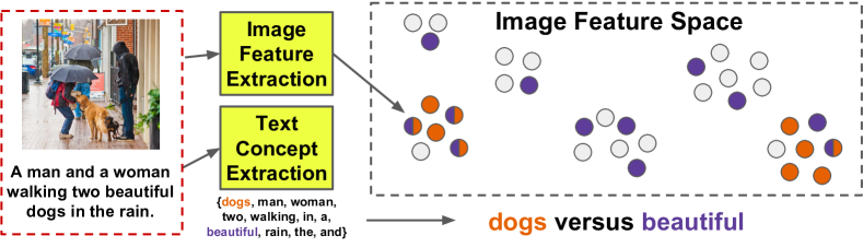
Figure 1: Demonstration of visual concreteness estimation on an example from the COCO dataset. The degree of visual clustering of textual concepts is measured using a nearest neighbor technique. The concreteness of “dogs” is greater than the concreteness of “beautiful” because images associated with “dogs” are packed tightly into two clusters, while images associated with “beautiful” are spread evenly.

Ideally, machine learning algorithms that incorporate information from both text and images should have a fuller perspective than those that consider either text or images in isolation. But Hill and Korhonen (2014b) observe that for their particular multimodal architecture, the level of concreteness of a concept being represented — intuitively, the idea of a dog is more concrete than that of beauty — affects whether multimodal or single-channel representations are more effective. In their case, concreteness was derived for 766 nouns and verbs from a fixed psycholinguistic database of human ratings.

In contrast, we introduce an adaptive algorithm for characterizing the visual concreteness of all the concepts indexed textually (e.g., “dog”) in a given multimodal dataset. Our approach is to leverage the geometry of image/text space. Intuitively, a visually concrete concept is one associated with more locally similar sets of images; for example, images associated with “dog” will likely contain dogs, whereas images associated with “beautiful” may contain flowers, sunsets, weddings, or an abundance of other possibilities — see Fig. 2.

Allowing concreteness to be dataset-specific is an important innovation because concreteness is contextual. For example, in one dataset we work with, our method scores “London” as highly concrete because of a preponderance of iconic London images in it, such as Big Ben and double-decker buses; whereas for a separate dataset, “London” is used as a geotag for diverse images, so the same word scores as highly non-concrete.

In addition to being dataset-specific, our method readily scales, does not depend on an external search engine, and is compatible with both discrete and continuous textual concepts (e.g., topic distributions).

Dataset-specific visual concreteness scores enable a variety of purposes. In this paper, we focus on using them to: 1) explore multimodal datasets; and 2) predict how easily concepts will be learned in a machine learning setting. We apply our method to four large multimodal datasets, ranging from image captions to image/text data scraped from Wikipedia, to examine the relationship between concreteness scores and the performance of machine learning algorithms. Specifically, we consider the cross-modal retrieval problem, and examine a number of NLP, vision, and retrieval algorithms. Across all 320 significantly different experimental settings (= 4 datasets $\times$ 2 image-representation algorithms $\times$ 5 textual-representation algorithms $\times$ 4 text/image alignment algorithms $\times$ 2 feature pre-processing schemes), we find that more concrete instances are easier to retrieve, and that different algorithms have similar failure cases. Interestingly, the relationship between concreteness and retrievability varies significantly based on dataset: some datasets appear to have a linear relationship between the two, whereas others exhibit a concreteness threshold beyond which retrieval becomes much easier.

We believe that our work can have a positive impact on future multimodal research. §8 gives more detail, but in brief, we see implications in (1) evaluation — more credit should perhaps be assigned to performance on non-concrete concepts; (2) creating or augmenting multimodal datasets, where one might a priori consider the desired relative proportion of concrete vs. non-concrete concepts; and (3) curriculum learning Bengio et al. (2009), where ordering of training examples could take concreteness levels into account.

2 Related Work

Applying machine learning to understand visual-textual relationships has enabled a number of new applications, e.g., better accessibility via automatic generation of alt text (Garcia et al., 2016), cheaper training-data acquisition for computer vision Joulin et al. (2016); Veit et al. (2017), and cross-modal retrieval systems, e.g., Rasiwasia et al. (2010); Costa Pereira et al. (2014).

Multimodal datasets often have substantially differing characteristics, and are used for different tasks (Baltrušaitis et al., 2017). Some commonly used datasets couple images with a handful of unordered tags (Barnard et al., 2003; Cusano et al., 2004; Grangier and Bengio, 2008; Chen et al., 2013, inter alia) or short, literal natural language captions (Farhadi et al., 2010; Ordóñez et al., 2011; Kulkarni et al., 2013; Fang et al., 2015, inter alia). In other cross-modal retrieval settings, images are paired with long, only loosely thematically-related documents. (Khan et al., 2009; Socher and Fei-Fei, 2010; Jia et al., 2011; Zhuang et al., 2013, inter alia). We provide experimental results on both types of data.

Concreteness in datasets has been previously studied in either text-only cases Turney et al. (2011); Hill et al. (2013) or by incorporating human judgments of perception into models Silberer and Lapata (2012); Hill and Korhonen (2014a). Other work has quantified characteristics of concreteness in multimodal datasets Young et al. (2014); Hill et al. (2014); Hill and Korhonen (2014b); Kiela and Bottou (2014); Jas and Parikh (2015); Lazaridou et al. (2015); Silberer et al. (2016); Lu et al. (2017); Bhaskar et al. (2017). Most related to our work is that of Kiela et al. Kiela et al. (2014); the authors use Google image search to collect 50 images each for a variety of words and compute the average cosine similarity between vector representations of returned images. In contrast, our method can be tuned to specific datasets without reliance on an external search engine. Other algorithmic advantages of our method include that: it more readily scales than previous solutions, it makes relatively few assumptions regarding the distribution of images/text, it normalizes for word frequency in a principled fashion, and it can produce confidence intervals. Finally, the method we propose can be applied to both discrete and continuous concepts like topic distributions.

3 Quantifying Visual Concreteness

To compute visual concreteness scores, we adopt the same general approach as Kiela et al. (2014): for a fixed text concept (i.e., a word or topic), we measure the variance in the corresponding visual features. The method is summarized in Figure 2.

3.1 Concreteness of discrete words

We assume as input a multimodal dataset of $n$ images represented in a space where nearest neighbors may be computed. Additionally, each image is associated with a set of discrete words/tags. We write $w_{v}$ for the set of words/tags associated with image $v$, and $V_{w}$ for the set of all images associated with a word $w$. For example, if the $v^{th}$ image is of a dog playing frisbee, $w_{v}$ might be $\{\text{frisbee},\text{dog},\text{in},\text{park}\}$, and $v\in V_{\text{park}}$.

Our goal is to measure how “clustered” a word is in image feature space. Specifically, we ask: for each image $v\in V_{w}$, how often are $v$’s nearest neighbors also associated with $w$? We thus compute the expected value of ${\rm MNI}^{k}_{w}$, the number of mutually neighboring images of word $w$:

$$\mathbb{E}_{P_{data}}[{\rm MNI}^{k}_{w}]=\frac{1}{|V_{w}|}\sum_{v\in V_{w}}|{\rm NN}^{k}(v)\cap V_{w}|\,,$$ (1)

where ${\rm NN}^{k}(v)$ denotes the set of $v$’s $k$ nearest neighbors in image space.

While Equation 1 measures clusteredness, it does not properly normalize for frequency. Consider a word like “and”; we expect it to have low concreteness, but its associated images will share neighbors simply because “and” is a frequent unigram. To correct for this, we compute the concreteness of a word as the ratio of $\mathbb{E}[{\rm MNI}^{k}_{w}]$ under the true distribution of the image data to a random distribution of the image data:

$$\text{concreteness}(w)=\frac{\mathbb{E}_{P_{data}}[{\rm MNI}^{k}_{w}]}{\mathbb{E}_{P_{random}}[{\rm MNI}^{k}_{w}]}$$ (2)

While the denominator of this expression can be computed in closed form, we use $\mathbb{E}_{P_{random}}[{\rm MNI}^{k}_{w}]\approx\frac{k|V_{w}|}{n}$; this approximation is faster to compute and is negligibly different from the true expectation in practice.

3.2 Extension to continuous topics

We extend the definition of concreteness to continuous concepts, so that our work applies also to topic model outputs; this extension is needed because the intersection in Equation 1 cannot be directly applied to real values. Assume we are given a set of topics $T$ and an image-by-topic matrix $Y\in\mathbb{R}^{n\times|T|}$, where the $v^{th}$ row is a topic distribution for the text associated with image $v$, i.e., $Y_{ij}=P(\text{topic }j|\text{image }i)$. For each topic $t$, we compute the average topic weight for each image $v$’s neighbors, and take a weighted average as:

$$\text{concreteness}(t)=\frac{n}{k}\cdot\frac{\sum_{v=1}^{n}[Y_{vt}\sum_{j\in{\rm NN}^{k}(v)}Y_{jt}]}{\left(\sum_{v=1}^{n}Y_{vt}\right)^{2}}$$ (3)

Note that Equations 1 and 3 are computations of means. Therefore, confidence intervals can be computed in both cases either using a normality assumption or bootstrapping.

4 Datasets

We consider four datasets that span a variety of multimodal settings. Two are publicly available and widely used (COCO/Flickr); we collected and preprocessed the other two (Wiki/BL). The Wikipedia and British Library sets are available for download at http://www.cs.cornell.edu/~jhessel/concreteness/concreteness.html. Dataset statistics are given in Table 1, and summarized as follows:

Figure 2: Examples of text and images from our new Wiki/BL datasets.

Wikipedia (Wiki). We collected a dataset consisting of 192K articles from the English Wikipedia, along with the 549K images contained in those articles. Following Wilson’s popularity filtering technique, we selected this subset of Wikipedia by identifying articles that received at least 50 views on March 5th, 2016. To our knowledge, the previous largest publicly available multimodal Wikipedia dataset comes from ImageCLEF’s 2011 retrieval task Popescu et al. (2010), which consists of 137K images associated with English articles.

	# Images	Mean Len	Train$/$	Test
Wiki	549K	$1397.8$	177K$/$	10K
BL	405K	$2269.6$	69K$/$	5K
COCO	123K	$10.5$	568K$/$	10K
Flickr	754K	$9.0$	744K$/$	10K

Table 1: Dataset statistics: total number of images, average text length in words, and size of the train/test splits we use in §6.

Images often appear on multiple pages: an image of the Eiffel tower might appear on pages for Paris, for Gustave Eiffel, and for the tower itself.

Historical Books from British Library (BL). The British Library has released a set of digitized books British Library Labs (2016) consisting of 25M pages of OCRed text, alongside 500K+ images scraped from those pages of text. The release splits images into four categories; we ignore “bound covers” and “embellishments” and use images identified as “plates” and “medium sized.” We associated images with all text within a 3-page window.

This raw data collection is noisy. Many books are not in English, some books contain far more images than others, and the images themselves are of varying size and rotation. To combat these issues we only keep books that have identifiably English text; for each cross-validation split in our machine-learning experiments (§6) we sample at most 10 images from each book; and we use book-level holdout so that no images/text in the test set are from books in the training set.

Captions and Tags. We also examine two popular existing datasets: Microsoft COCO (captions) Lin et al. (2014) (COCO) and MIRFLICKR-1M (tags) Huiskes et al. (2010) (Flickr). For COCO, we construct our own training/validation splits from the 123K images, each of which has 5 captions. For Flickr, as an initial preprocessing step we only consider the 7.3K tags that appear at least 200 times, and the 754K images that are associated with at least 3 of the 7.3K valid tags.

5 Validation of Concreteness Scoring

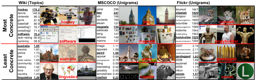
Figure 3: Examples of the most and least concrete words/topics from Wiki, COCO, and Flickr, along with example images associated with each highlighted word/topic.

We apply our concreteness measure to the four datasets. For COCO and Flickr, we use unigrams as concepts, while for Wiki and BL, we extract 256-dimensional topic distributions using Latent Dirichlet Allocation (LDA) Blei et al. (2003). For BL, topic distributions are derived from text in the aforementioned 3 page window; for Wiki, for each image, we compute the mean topic distribution of all articles that image appears in; for Flickr, we associate images with all of their tags; for COCO, we concatenate all captions for a given image. For computing concreteness scores for COCO/Flickr, we only consider unigrams associated with at least 100 images, so as to ensure the stability of MNI as defined in Equation 1.

We extract image features from the pre-softmax layer of a deep convolutional neural network, ResNet50 He et al. (2016), pretrained for the ImageNet classification task Deng et al. (2009); this method is known to be a strong baseline Sharif Razavian et al. (2014). For nearest neighbor search, we use the Annoy library, which computes approximate kNN efficiently. We use $k=50$ nearest neighbors, though the results presented are stable for reasonable choices of $k$, e.g., $k=25,100$.

5.1 Concreteness and human judgments

Following Kiela et al. Kiela et al. (2014), we borrow a dataset of human judgments to validate our concreteness computation method. The concreteness of words is a topic of interest in psychology because concreteness relates to a variety of aspects of human behavior, e.g., language acquisition, memory, etc. Schwanenflugel and Shoben (1983); Paivio (1991); Walker and Hulme (1999); De Groot and Keijzer (2000).

We compare against the human-gathered unigram concreteness judgments provided in the USF Norms dataset (USF) Nelson et al. (2004); for each unigram, raters provided judgments of its concreteness on a 1-7 scale. For Flickr/COCO, we compute Spearman correlation using these per-unigram scores (the vocabulary overlap between USF and Flickr/COCO is 1.3K/1.6K), and for Wiki/BL, we compute topic-level human judgment scores via a simple average amongst the top 100 most probable words in the topic.

As a null hypothesis, we consider the possibility that our concreteness measure is simply mirroring frequency information. We measure frequency for each dataset by measuring how often a particular word/topic appears in it. A useful concreteness measure should correlate with USF more than a simple frequency baseline does.

For COCO/Flickr/Wiki, concreteness scores output by our method positively correlate with human judgments of concreteness more than frequency does (see Figure 4). For COCO, this pattern holds even when controlling for part-of-speech (not shown), whereas Flickr adjectives are not correlated with USF. For BL, neither frequency nor our concreteness scores are significantly correlated with USF. Thus, in three of our four datasets, our measure tends to predict human concreteness judgments better than frequency.

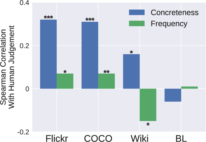
Figure 4: Spearman correlations between human judgment (USF) and our algorithm’s outputs, and dataset frequency. In the case of Flickr/COCO/WIKI our concreteness scores correlate with human judgement to a greater extent than frequency. For BL, neither frequency nor our concreteness measure is correlated with human judgement. ***/**/* := $p<.001/.01/.05$

Concreteness and frequency. While concreteness measures correlate with human judgment better than frequency, we do expect some correlation between a word’s frequency and its concreteness Gorman (1961). In all cases, we observe a moderate-to-strong positive correlation between infrequency and concreteness ($\rho_{wiki},\rho_{coco},\rho_{flickr},\rho_{bl}=.06,.35,.40,.71$) indicating that rarer words/topics are more concrete, in general. However, the correlation is not perfect, and concreteness and frequency measure different properties of words.

5.2 Concreteness within datasets

Figure 3 gives examples from Wiki, COCO, and Flickr illustrating the concepts associated with the smallest and largest concreteness scores according to our method. The scores often align with intuition, e.g., for Wiki, sports topics are often concrete, whereas country-based or abstract-idea-based topics are not. For COCO, polar (because of polar bears) and ben (because of Big Ben) are concrete; whereas somewhere and possibly are associated with a wide variety of images.

Concreteness scores form a continuum, making explicit not only the extrema (as in Figure 3) but also the middle ground, e.g., in COCO, “wilderness” (rank 479) is more visually concrete than “outside” (rank 2012). Also, dataset-specific intricacies that are not obvious a priori are highlighted, e.g., in COCO, 150/151 references to “magnets” (rank 6) are in the visual context of a refrigerator (making “magnets” visually concrete) though the converse is not true, as both “refrigerator” (rank 329) and “fridge” (rank 272) often appear without magnets; 61 captions in COCO are exactly “There is no image here to provide a caption for,” and this dataset error is made explicit through concreteness score computations.

5.3 Concreteness varies across datasets

To what extent are the concreteness scores dataset-specific? To investigate this question, we compute the correlation between Flickr and COCO unigram concreteness scores for 1129 overlapping terms. While the two are positively correlated ($\rho=.48,p<.01$) there are many exceptions that highlight the utility of computing dataset-independent scores. For instance, “London” is extremely concrete in COCO (rank 9) as compared to in Flickr (rank 1110). In COCO, images of London tend to be iconic (i.e., Big Ben, double decker buses); in contrast, “London” often serves as a geotag for a wider variety of images in Flickr. Conversely, “watch” in Flickr is concrete (rank 196) as it tends to refer to the timepiece, whereas “watch” is not concrete in COCO (rank 958) as it tends to refer to the verb; while these relationships are not obvious a priori, our concreteness method has helped to highlight these usage differences between the image tagging and captioning datasets.

6 Learning Image/Text Correspondences

Previous work suggests that incorporating visual features for less concrete concepts can be harmful in word similarity tasks Hill and Korhonen (2014b); Kiela et al. (2014); Kiela and Bottou (2014); Hill et al. (2014). However, it is less clear if this intuition applies to more practical tasks (e.g., retrieval), or if this problem can be overcome simply by applying the “right” machine learning algorithm. We aim to tackle these questions in this section.

The learning task. The task we consider is the construction of a joint embedding of images and text into a shared vector space. Truly corresponding image/text pairs (e.g., if the text is a caption of that image) should be placed close together in the new space relative to image/text pairs that do not match. This task is a good representative of multimodal learning because computing a joint embedding of text and images is often a “first step” for downstream tasks, e.g., cross-modal retrieval Rasiwasia et al. (2010), image tagging Chen et al. (2013), and caption generation Kiros et al. (2015).

Evaluations. Following previous work in cross-modal retrieval, we measure performance using the top-$k\%$ hit rate (also called recall-at-$k$-percent, $R@k\%$; higher is better). Cross-modal retrieval can be applied in either direction, i.e., searching for an image given a body of text, or vice-versa. We examine both the image-search-text and text-search-image cases . For simplicity, we average retrieval performance from both directions, producing a single metric; higher is better.

Visual Representations. Echoing Wei et al. (2016), we find that features extracted from convolutional neural networks (CNNs) outperform classical computer vision descriptors (e.g., color histograms) for multimodal retrieval. We consider two different CNNs pretrained on different datasets: ResNet50 features trained on the ImageNet classification task (RN-Imagenet), and InceptionV3 Szegedy et al. (2015) trained on the OpenImages Krasin et al. (2017) image tagging task (I3-OpenImages).

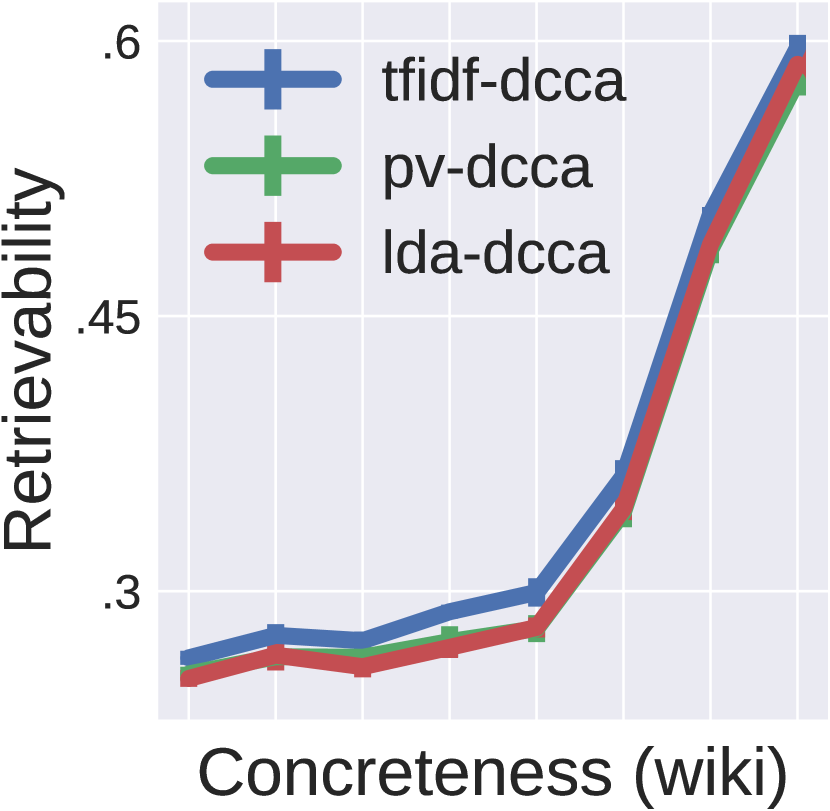
	NP	LS	NS	DCCA
BTM	14.1	19.8	20.7	27.9
LDA	19.8	36.2	33.1	37.0
PV	22.0	30.8	29.4	37.1
uni	17.3	29.3	30.2	36.3
tfidf	18.1	35.2	33.2	38.7

(a) Wikipedia

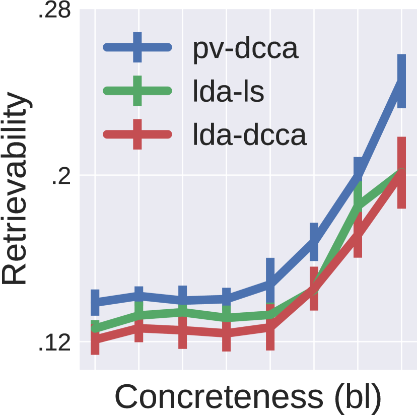
	NP	LS	NS	DCCA
BTM	6.7	7.3	7.2	9.5
LDA	10.2	17.1	13.8	16.4
PV	12.6	14.1	14.1	17.8
uni	11.0	13.2	12.4	15.6
tfidf	10.9	15.1	13.5	15.5

(b) British Library

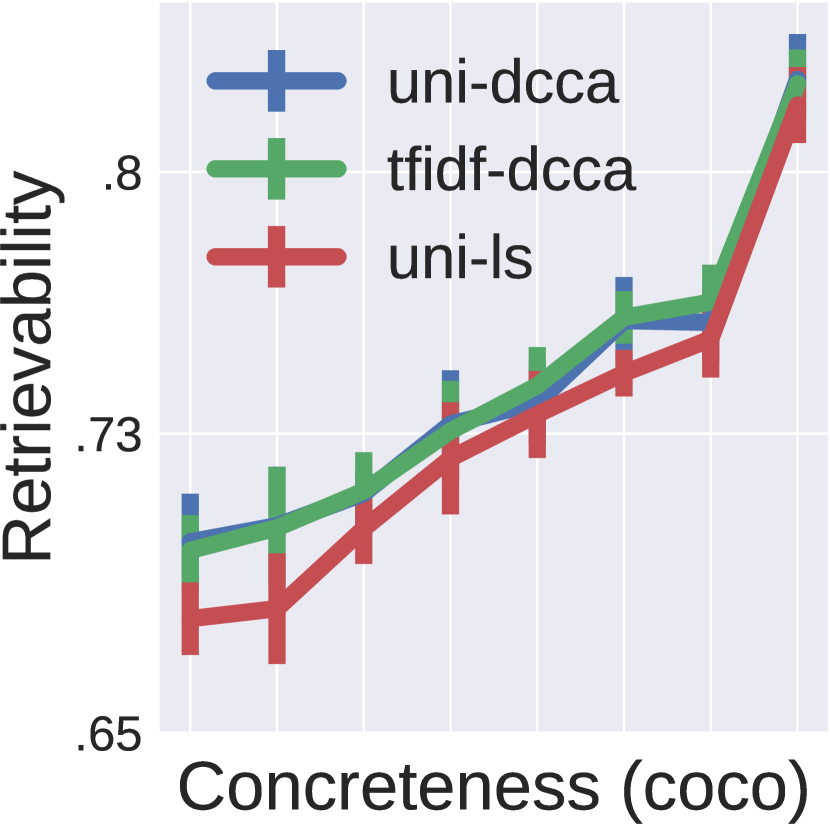
	NP	LS	NS	DCCA
BTM	27.3	39.9	52.5	58.6
LDA	23.2	51.6	51.9	51.8
PV	14.1	28.4	25.7	33.5
uni	28.7	74.6	72.5	75.0
tfidf	32.9	74.0	74.1	74.9

(c) COCO

	NP	LS	NS	DCCA
BTM	23.9	19.1	31.0	32.4
LDA	18.4	32.2	34.4	34.7
PV	13.9	21.3	20.0	26.6
uni	34.7	62.5	62.0	59.6
tfidf	35.1	61.6	63.9	60.2

(d) Flickr

Figure 5: Concreteness scores versus retrievability (plotted) for each dataset, along with Recall at 1% (in tables, higher is better) for each algorithm combination. Tables give average retrieval performance over 10-fold cross-validation for each combination of NLP/alignment algorithm; the best, second best, and third best performing combinations are bolded and colored. The concreteness versus retrievability curves are plotted for the top-3 performing algorithms, though similar results hold for all algorithms. Our concreteness scores and performance are positively correlated, though the shape of the relationship between the two differs from dataset to dataset (note the differing scales of the y-axes). All results are for RN-ImageNet; the similar I3-OpenImages results are omitted for space reasons.

Text Representations. We consider sparse unigram and tfidf indicator vectors. In both cases, we limit the vocabulary size to 7.5K. We next consider latent-variable bag-of-words models, including LDA Blei et al. (2003) (256 topics, trained with Mallet McCallum (2002)) a specialized biterm topic model (BTM) Yan et al. (2013) for short texts (30 topics), and paragraph vectors (PV) Le and Mikolov (2014) (PV-DBOW version, 256 dimensions, trained with Gensim Řehůřek and Sojka (2010)).

Alignment of Text and Images. We explore four algorithms for learning correspondences between image and text vectors. We first compare against Hodosh et al. (2013)’s nonparametric baseline (NP), which is akin to a nearest-neighbor search. This algorithm is related to the concreteness score algorithm we previously introduced in that it exploits the geometry of the image/text spaces using nearest-neighbor techniques. In general, performance metrics for this algorithm provide an estimate of how “easy” a particular task is in terms of the initial image/text representations.

We next map image features to text features via a simple linear transformation. Let $(t_{i},v_{i})$ be a text/image pair in the dataset. We learn a linear transformation $W$ that minimizes

$$\sum_{i}\|Wf_{\text{image}}(v_{i})-f_{\text{text}}(t_{i})\|_{2}^{2}+\lambda\|W\|_{F}$$ (4)

for feature extraction functions $f_{\text{image}}$ and $f_{\text{text}}$, e.g., RN-ImageNet/LDA. It is possible to map images onto text as in Equation 4, or map text onto images in an analogous fashion. We find that the directionality of the mapping is important. We train models in both directions, and combine their best-performing results into a single least-squares (LS) model.

Next we consider Negative Sampling (NS), which balances two objectives: true image/text pairs should be close in the shared latent space, while randomly combined image/text pairs should be far apart. For a text/image pair $(t_{i},v_{i})$, let $s(t_{i},v_{i})$ be the cosine similarity of the pair in the shared space. The loss for a single positive example $(t_{i},v_{i})$ given a negative sample $(t_{i}^{\prime},v_{i}^{\prime})$ is

$$h\bigl{(}s(t_{i},v_{i}),s(t_{i},v_{i}^{\prime})\bigr{)}+h\bigl{(}s(t_{i},v_{i}),s(t_{i}^{\prime},v_{i})\bigr{)}$$ (5)

for the hinge function $h(p,n)=\max\{0,\alpha-p+n\}$. Following Kiros et al. (2015) we set $\alpha=.2$.

Finally, we consider Canonical Correlation Analysis (CCA), which projects image and text representations down to independent dimensions of high multimodal correlation. CCA-based methods are popular within the IR community for learning multimodal embeddings Costa Pereira et al. (2014); Gong et al. (2014). We use Wang et al. (2015b)’s stochastic method for training deep CCA Andrew et al. (2013) (DCCA), a method that is competitive with traditional kernel CCA Wang et al. (2015a) but less memory-intensive to train.

Training details. LS, NS, and DCCA were implemented using Keras Chollet et al. (2015). In total, we examine all combinations of: four datasets, five NLP algorithms, two vision algorithms, four cross-modal alignment algorithms, and two feature preprocessing settings; each combination was run using 10-fold cross-validation.

Absolute retrieval quality. The tables in Figure 5 contain the retrieval results for RN-ImageNet image features across each dataset, alignment algorithm, and text representation scheme. We show results for $R@1\%$, but $R@5\%$ and $R@10\%$ are similar. I3-OpenImages image features underperform relative to RN-ImageNet and are omitted for space reasons, though the results are similar.

The BL corpus is the most difficult of the datasets we consider, yielding the lowest retrieval scores. The highly-curated COCO dataset appears to be the easiest, followed by Flickr and then Wikipedia. No single algorithm combination is “best” in all cases.

6.1 Concreteness scores and performance

We now examine the relationship between retrieval performance and concreteness scores. Because concreteness scores are on the word/topic level, we define a retrievability metric that summarizes an algorithm’s performance on a given concept; for example, we might expect that $\text{retrievability}(\text{dog})$ is greater than $\text{retrievability}(\text{beautiful})$.

Borrowing the $R@1\%$ metric from the previous section, we let $\mathbb{I}[r_{i}<1\%]$ be an indicator variable indicating that test instance $i$ was retrieved correctly, i.e., $\mathbb{I}[r_{i}<1\%]$ is 1 if the the average rank $r_{i}$ of the image-search-text/text-search-image directions is better than $1\%$, and 0 otherwise. Let $s_{ic}$ be the affinity of test instance $i$ to concept $c$. In the case of topic distributions, $s_{ic}$ is the proportion of topic $c$ in instance $i$; in the case of unigrams, $s_{ic}$ is the length-normalized count of unigram $c$ on instance $i$. Retrievability is defined using a weighted average over test instances $i$ as:

$$\text{retrievability}(c)=\frac{\sum_{i}s_{ic}\cdot\mathbb{I}[r_{i}<1\%]}{\sum_{i}s_{ic}}$$ (6)

The retrievability of $c$ will be higher if instances more associated with $c$ are more easily retrieved by the algorithm.

Retrievability vs. Concreteness. The graphs in Figure 5 plot our concreteness scores versus retrievability of the top 3 performing NLP/alignment algorithm combinations for all 4 datasets. In all cases, there is a strong positive correlation between concreteness and retrievability, which provides evidence that more concrete concepts are easier to retrieve.

The shape of the concreteness-retrievability curve appears to vary between datasets more than between algorithms. In COCO, the relationship between the two appears to smoothly increase. In Wiki, on the other hand, there appears to be a concreteness threshold, beyond which retrieval becomes much easier.

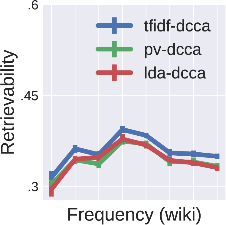
(a) Wikipedia

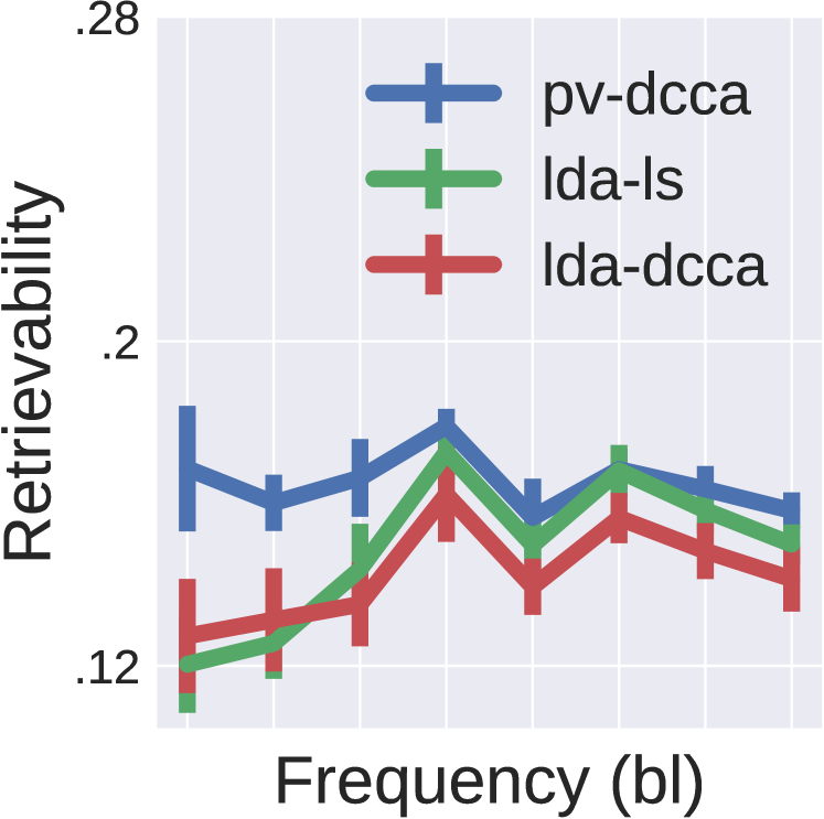
(b) British Library

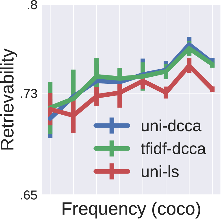
(c) COCO

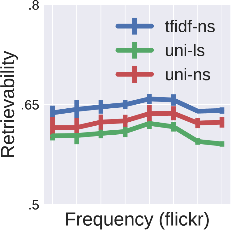
(d) Flickr

Figure 6: Correlation between word/topic frequency and retrievability for each of the four datasets. Compared to our concreteness measure (see Figure 5; note that the while x-axes are different, the y-axes are the same) frequency explains relatively little variance in retrievability.

There is little relationship between retrievability and frequency, further suggesting that our concreteness measure is not simply mirroring frequency. We re-made the plots in Figure 5, except we swapped the x-axis from concreteness to frequency; the resulting plots, given in Figure 6, are much flatter, indicating that retrievability and frequency are mostly uncorrelated. Additional regression analyses reveal that for the top-3 performing algorithms on Flickr/Wiki/BL/COCO, concreteness explains 33%/64%/11%/15% of the variance in retrievability, respectively. In contrast, for all datasets, frequency explained less than 1% of the variance in retrievability.

7 Beyond Cross-Modal Retrieval

Concreteness scores do more than just predict retrieval performance; they also predict the difficulty of image classification. Two popular shared tasks from the ImageNet 2015 competition published class-level errors of all entered systems. We used the unigram concreteness scores from Flickr/COCO computed in §3 to derive concreteness scores for the ImageNet classes. We find that for both classification and localization, for all 10 top performing entries, and for both Flickr/COCO, there exists a moderate-to-strong Spearman correlation between concreteness and performance among the classes for which concreteness scores were available ($n_{\text{flickr}},n_{\text{coco}}=171,288$; $.18<\rho<.44$; $p<.003$ in all cases). This result suggests that concrete concepts may tend to be easier on tasks other than retrieval, as well.

8 Future Directions

At present, it remains unclear if abstract concepts should be viewed as noise to be discarded (as in Kiela et al. Kiela et al. (2014)), or more difficult, but learnable, signal. Because large datasets (e.g., social media) increasingly mix modalities using ambiguous, abstract language, researchers will need to tackle this question going forward. We hope that visual concreteness scores can guide investigations of the trickiest aspects of multimodal tasks. Our work suggests the following future directions:

Evaluating algorithms: Because concreteness scores are able to predict performance prior to training, evaluations could be reported over concrete and abstract instances separately, as opposed to aggregating into a single performance metric. A new algorithm that consistently performs well on non-concrete concepts, even at the expense of performance on concrete concepts, would represent a significant advance in multimodal learning.

Designing datasets: When constructing a new multimodal dataset, or augmenting an existing one, concreteness scores can offer insights regarding how resources should be allocated. Most directly, these scores enable focusing on “concrete visual concepts” Huiskes et al. (2010); Chen et al. (2015), by issuing image-search queries could be issued exclusively for concrete concepts during dataset construction. The opposite approach could also be employed, by prioritizing less concrete concepts.

Curriculum learning: During training, instances could be up/down-weighted in the training process in accordance with concreteness scores. It is not clear if placing more weight on the trickier cases (down-weighting concreteness), or giving up on the harder instances (up-weighting concreteness) would lead to better performance, or differing algorithm behavior.

9 Acknowledgments

This work was supported in part by NSF grants SES-1741441/IIS-1652536/IIS-1526155, a Yahoo Faculty Research and Engagement Program grant, the Alfred P. Sloan Foundation, and a Cornell Library Grant. Any opinions, findings, and conclusions or recommendations expressed in this material are those of the authors and do not necessarily reflect the views of the NSF, Sloan Foundation, Yahoo, or other sponsors. Nvidia kindly provided the Titan X GPU used in this work.

We would additionally like to thank Maria Antoniak, Amit Bahl, Jeffrey Chen, Bharath Hariharan, Arzoo Katiyar, Vlad Niculae, Xanda Schofield, Laure Thompson, Shaomei Wu, and the anonymous reviewers for their constructive comments.

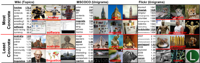
Figure 7: Images in this figure are reproduced in accordance with the following licensing information. The original authors of the images do not necessarily endorse this work or the opinions expressed in it. Copyright information is given left-to-right. Wikipedia: “hockey” – Dan4th Nicholas (CC BY 2.0); Leech44 (CC BY 3.0); Usasoccer2010 (CC BY-SA 3.0). All “software” images derive from software licensed under GNU GPL v3; screenshot used under fair use. “Australia” – Toby Hudson (CC BY-SA 3.0); public domain; public domain. “linguistics” – Suasysar (public domain); USDA (public domain); Rama (CC BY-SA 2.0 FR). MSCOCO: “ben” – Michael Garnett (CC BY-NC-ND 2.0); Giovanni Tufo (CC BY-NC-ND 2.0); Edinho Souto (CC BY-NC-SA 2.0). “magnets” – Gabriel Pires (CC BY-NC-SA 2.0); the_blue (CC BY-NC-SA 2.0); Dennis S. Hurd (CC BY-NC-ND 2.0) “weird” – waferboard (CC BY 2.0); jaci XIII (CC BY-NC-SA 2.0); Ozzy Delaney (CC BY 2.0). “caption” – Robert G. Daigle (CC BY 2.0) TJ Gehling (CC BY-NC-ND 2.0); amhuxham (CC BY-NC-SA 2.0). Flickr: “cheetah” – Nathan Rupert (CC BY-NC-ND 2.0); Karen Dorsett (CC BY-ND 2.0); Vearl Brown (CC BY-NC 2.0). “bodybuilder” – Kent (SSCusp) (CC BY-NC-ND 2.0); Frank Carroll (CC BY-NC-SA 2.0); Kent (SSCusp) (CC BY-NC-ND 2.0). “geotagged” – tpholland (CC BY 2.0); s2art (CC BY-NC-SA 2.0); Joe Penniston (CC BY-NC-ND 2.0). “canon” – ajagendorf25 (CC BY 2.0); Tom Lin (CC BY-NC-ND 2.0); Leo Reynolds (CC BY-NC-SA 2.0).

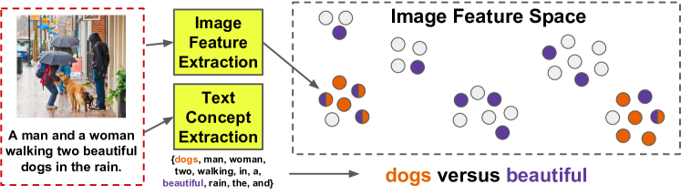
Figure 8: Images in this figure are reproduced in accordance with the following licensing information. The original authors of the images do not necessarily endorse this work or the opinions expressed in it. J. Michel (aka: Mitch) Carriere (CC BY-NC-ND 2.0)

Figure 9: Images in this figure are reproduced in accordance with the following licensing information. The original authors of the images do not necessarily endorse this work or the opinions expressed in it. Wiki – US Air Force (public domain); Fairsing (public domain). The BL images are also public domain, and were originally released by the british library.

References

- Andrew et al. (2013) Galen Andrew, Raman Arora, Jeff A. Bilmes, and Karen Livescu. 2013. Deep canonical correlation analysis. In ICML.
- Baltrušaitis et al. (2017) Tadas Baltrušaitis, Chaitanya Ahuja, and Louis-Philippe Morency. 2017. Multimodal machine learning: A survey and taxonomy. arXiv preprint 1705.09406.
- Barnard et al. (2003) Kobus Barnard, Pinar Duygulu, David Forsyth, Nando De Freitas, David M. Blei, and Michael I. Jordan. 2003. Matching words and pictures. JMLR.
- Bengio et al. (2009) Yoshua Bengio, Jérôme Louradour, Ronan Collobert, and Jason Weston. 2009. Curriculum learning. In ICML.
- Bhaskar et al. (2017) Sai Abishek Bhaskar, Maximilian Köper, Sabine Schulte im Walde, and Diego Frassinelli. 2017. Exploring multi-modal text+image models to distinguish between abstract and concrete nouns. In IWCS Workshop on Foundations of Situated and Multimodal Communication.
- Blei et al. (2003) David M. Blei, Andrew Y. Ng, and Michael I. Jordan. 2003. Latent Dirichlet allocation. JMLR.
- British Library Labs (2016) British Library Labs. 2016. Digitised books. https://data.bl.uk/digbks/.
- Chen et al. (2013) Minmin Chen, Alice X. Zheng, and Kilian Q. Weinberger. 2013. Fast image tagging. In ICML.
- Chen et al. (2015) Xinlei Chen, Hao Fang, Tsung-Yi Lin, Ramakrishna Vedantam, Saurabh Gupta, Piotr Dollár, and C. Lawrence Zitnick. 2015. Microsoft COCO captions: Data collection and evaluation server. arXiv preprint arXiv:1504.00325.
- Chollet et al. (2015) François Chollet et al. 2015. Keras. https://github.com/fchollet/keras.
- Costa Pereira et al. (2014) Jose Costa Pereira, Emanuele Coviello, Gabriel Doyle, Nikhil Rasiwasia, Gert R.G. Lanckriet, Roger Levy, and Nuno Vasconcelos. 2014. On the role of correlation and abstraction in cross-modal multimedia retrieval. TPAMI.
- Cusano et al. (2004) Claudio Cusano, Gianluigi Ciocca, and Raimondo Schettini. 2004. Image annotation using SVM. In Electronic Imaging.
- De Groot and Keijzer (2000) Annette De Groot and Rineke Keijzer. 2000. What is hard to learn is easy to forget: The roles of word concreteness, cognate status, and word frequency in foreign-language vocabulary learning and forgetting. Language Learning, 50(1):1–56.
- Deng et al. (2009) Jia Deng, Wei Dong, Richard Socher, Li-Jia Li, Kai Li, and Li Fei-Fei. 2009. ImageNet: A large-scale hierarchical image database. In CVPR.
- Fang et al. (2015) Hao Fang, Saurabh Gupta, Forrest Iandola, Rupesh K. Srivastava, Li Deng, Piotr Dollár, Jianfeng Gao, Xiaodong He, Margaret Mitchell, John C. Platt, C. Lawrence Zitnick, and Geoffrey Zweig. 2015. From captions to visual concepts and back. In CVPR.
- Farhadi et al. (2010) Ali Farhadi, Mohsen Hejrati, Mohammad Amin Sadeghi, Peter Young, Cyrus Rashtchian, Julia Hockenmaier, and David Forsyth. 2010. Every picture tells a story: Generating sentences from images. In ECCV.
- Garcia et al. (2016) Dario Garcia Garcia, Manohar Paluri, and Shaomei Wu. 2016. Under the hood: Building accessibility tools for the visually impaired on facebook. https://code.facebook.com/posts/457605107772545/under-the-hood-building-accessibility-tools-for-the-visually-impaired-on-facebook/.
- Gong et al. (2014) Yunchao Gong, Qifa Ke, Michael Isard, and Svetlana Lazebnik. 2014. A multi-view embedding space for modeling internet images, tags, and their semantics. IJCV.
- Gorman (1961) Aloysia M. Gorman. 1961. Recognition memory for nouns as a function of abstractness and frequency. Journal of Experimental Psychology, 61(1):23–29.
- Grangier and Bengio (2008) David Grangier and Samy Bengio. 2008. A discriminative kernel-based approach to rank images from text queries. TPAMI.
- He et al. (2016) Kaiming He, Xiangyu Zhang, Shaoqing Ren, and Jian Sun. 2016. Deep residual learning for image recognition. In CVPR.
- Hill et al. (2013) Felix Hill, Douwe Kiela, and Anna Korhonen. 2013. Concreteness and corpora: A theoretical and practical analysis. In Workshop on Cognitive Modeling and Computational Linguistics.
- Hill and Korhonen (2014a) Felix Hill and Anna Korhonen. 2014a. Concreteness and subjectivity as dimensions of lexical meaning. In ACL, pages 725–731.
- Hill and Korhonen (2014b) Felix Hill and Anna Korhonen. 2014b. Learning abstract concept embeddings from multi-modal data: Since you probably can’t see what I mean. In EMNLP.
- Hill et al. (2014) Felix Hill, Roi Reichart, and Anna Korhonen. 2014. Multi-modal models for concrete and abstract concept meaning. TACL.
- Hodosh et al. (2013) Micah Hodosh, Peter Young, and Julia Hockenmaier. 2013. Framing image description as a ranking task: Data, models and evaluation metrics. JAIR.
- Huiskes et al. (2010) Mark J. Huiskes, Bart Thomee, and Michael S. Lew. 2010. New trends and ideas in visual concept detection: the MIR flickr retrieval evaluation initiative. In ACM MIR.
- Ioffe and Szegedy (2015) Sergey Ioffe and Christian Szegedy. 2015. Batch normalization: Accelerating deep network training by reducing internal covariate shift. JMLR.
- Jas and Parikh (2015) Mainak Jas and Devi Parikh. 2015. Image specificity. In CVPR.
- Jia et al. (2011) Yangqing Jia, Mathieu Salzmann, and Trevor Darrell. 2011. Learning cross-modality similarity for multinomial data. In ICCV.
- Joulin et al. (2016) Armand Joulin, Laurens van der Maaten, Allan Jabri, and Nicolas Vasilache. 2016. Learning visual features from large weakly supervised data. In ECCV.
- Khan et al. (2009) Inayatullah Khan, Amir Saffari, and Horst Bischof. 2009. TVGraz: Multi-modal learning of object categories by combining textual and visual features. In Workshop of the Austrian Association for Pattern Recognition.
- Kiela and Bottou (2014) Douwe Kiela and Léon Bottou. 2014. Learning image embeddings using convolutional neural networks for improved multi-modal semantics. In EMNLP.
- Kiela et al. (2014) Douwe Kiela, Felix Hill, Anna Korhonen, and Stephen Clark. 2014. Improving multi-modal representations using image dispersion: Why less is sometimes more. In ACL.
- Kingma and Ba (2015) Diederik Kingma and Jimmy Ba. 2015. Adam: A method for stochastic optimization. In ICLR.
- Kiros et al. (2015) Ryan Kiros, Ruslan Salakhutdinov, and Richard S. Zemel. 2015. Unifying visual-semantic embeddings with multimodal neural language models. TACL.
- Krasin et al. (2017) Ivan Krasin, Tom Duerig, Neil Alldrin, Vittorio Ferrari, Sami Abu-El-Haija, Alina Kuznetsova, Hassan Rom, Jasper Uijlings, Stefan Popov, Andreas Veit, Serge Belongie, Victor Gomes, Abhinav Gupta, Chen Sun, Gal Chechik, David Cai, Zheyun Feng, Dhyanesh Narayanan, and Kevin Murphy. 2017. OpenImages: A public dataset for large-scale multi-label and multi-class image classification. Dataset available from https://github.com/openimages.
- Kulkarni et al. (2013) Girish Kulkarni, Visruth Premraj, Vicente Ordóñez, Sagnik Dhar, Siming Li, Yejin Choi, Alexander C. Berg, and Tamara L. Berg. 2013. Babytalk: Understanding and generating simple image descriptions. TPAMI.
- Lazaridou et al. (2015) Angeliki Lazaridou, Nghia The Pham, and Marco Baroni. 2015. Combining language and vision with a multimodal skip-gram model. In NAACL.
- Le and Mikolov (2014) Quoc V. Le and Tomas Mikolov. 2014. Distributed representations of sentences and documents. In ICML.
- Lin et al. (2014) Tsung-Yi Lin, Michael Maire, Serge Belongie, James Hays, Pietro Perona, Deva Ramanan, Piotr Dollár, and C. Lawrence Zitnick. 2014. Microsoft COCO: Common objects in context. In ECCV.
- Lu et al. (2017) Jiasen Lu, Caiming Xiong, Devi Parikh, and Richard Socher. 2017. Knowing when to look: Adaptive attention via a visual sentinel for image captioning.
- McCallum (2002) Andrew Kachites McCallum. 2002. Mallet: A machine learning for language toolkit. http://mallet.cs.umass.edu.
- Nelson et al. (2004) Douglas L. Nelson, Cathy L. McEvoy, and Thomas A. Schreiber. 2004. The University of South Florida free association, rhyme, and word fragment norms. Behavior Research Methods, Instruments, & Computers, 36(3):402–407.
- Ordóñez et al. (2011) Vicente Ordóñez, Girish Kulkarni, and Tamara L. Berg. 2011. Im2text: Describing images using 1 million captioned photographs. In NIPS.
- Paivio (1991) Allan Paivio. 1991. Dual coding theory: Retrospect and current status. Canadian Journal of Psychology, 45(3):255–287.
- Popescu et al. (2010) Adrian Popescu, Theodora Tsikrika, and Jana Kludas. 2010. Overview of the Wikipedia retrieval task at ImageCLEF 2010. In CLEF.
- Rasiwasia et al. (2010) Nikhil Rasiwasia, Jose Costa Pereira, Emanuele Coviello, Gabriel Doyle, Gert R.G. Lanckriet, Roger Levy, and Nuno Vasconcelos. 2010. A new approach to cross-modal multimedia retrieval. In ACM MM.
- Řehůřek and Sojka (2010) Radim Řehůřek and Petr Sojka. 2010. Software framework for topic modelling with large corpora. In LREC Workshop on NLP Frameworks.
- Schwanenflugel and Shoben (1983) Paula J. Schwanenflugel and Edward J. Shoben. 1983. Differential context effects in the comprehension of abstract and concrete verbal materials. Journal of Experimental Psychology: Learning, Memory, and Cognition, 9(1):82–102.
- Sharif Razavian et al. (2014) Ali Sharif Razavian, Hossein Azizpour, Josephine Sullivan, and Stefan Carlsson. 2014. CNN features off-the-shelf: an astounding baseline for recognition. In CVPR Workshop.
- Silberer et al. (2016) Carina Silberer, Vittorio Ferrari, and Mirella Lapata. 2016. Visually grounded meaning representations. TPAMI.
- Silberer and Lapata (2012) Carina Silberer and Mirella Lapata. 2012. Grounded models of semantic representation. In EMNLP.
- Socher and Fei-Fei (2010) Richard Socher and Li Fei-Fei. 2010. Connecting modalities: Semi-supervised segmentation and annotation of images using unaligned text corpora. In CVPR.
- Szegedy et al. (2015) Christian Szegedy, Wei Liu, Yangqing Jia, Pierre Sermanet, Scott Reed, Dragomir Anguelov, Dumitru Erhan, Vincent Vanhoucke, and Andrew Rabinovich. 2015. Going deeper with convolutions. In CVPR.
- Turney et al. (2011) Peter D. Turney, Yair Neuman, Dan Assaf, and Yohai Cohen. 2011. Literal and metaphorical sense identification through concrete and abstract context. In EMNLP.
- Veit et al. (2017) Andreas Veit, Neil Alldrin, Gal Chechik, Ivan Krasin, Abhinav Gupta, and Serge Belongie. 2017. Learning from noisy large-scale datasets with minimal supervision. In CVPR.
- Walker and Hulme (1999) Ian Walker and Charles Hulme. 1999. Concrete words are easier to recall than abstract words: Evidence for a semantic contribution to short-term serial recall. Journal of Experimental Psychology: Learning, Memory, and Cognition, 25(5):1256–1271.
- Wang et al. (2015a) Weiran Wang, Raman Arora, Karen Livescu, and Jeff A. Bilmes. 2015a. On deep multi-view representation learning. In ICML.
- Wang et al. (2015b) Weiran Wang, Raman Arora, Karen Livescu, and Nathan Srebro. 2015b. Stochastic optimization for deep cca via nonlinear orthogonal iterations. In Communication, Control, and Computing.
- Wei et al. (2016) Yunchao Wei, Yao Zhao, Canyi Lu, Shikui Wei, Luoqi Liu, Zhenfeng Zhu, and Shuicheng Yan. 2016. Cross-modal retrieval with cnn visual features: A new baseline. Transactions on Cybernetics.
- Yan et al. (2013) Xiaohui Yan, Jiafeng Guo, Yanyan Lan, and Xueqi Cheng. 2013. A biterm topic model for short texts. In WWW.
- Young et al. (2014) Peter Young, Alice Lai, Micah Hodosh, and Julia Hockenmaier. 2014. From image descriptions to visual denotations: New similarity metrics for semantic inference over event descriptions. TACL.
- Zhuang et al. (2013) Yue Ting Zhuang, Yan Fei Wang, Fei Wu, Yin Zhang, and Wei Ming Lu. 2013. Supervised coupled dictionary learning with group structures for multi-modal retrieval. In AAAI.