Long-Horizon Forecasting Using Deep Learning

Long-Horizon Forecasting Using Deep Learning

Abstract

Existing forecasting methods based on deep Recurrent Neural Networks (DeepRNN) target short term predictions, e.g given a set of features predict some output for the next time step or a couple steps in the future. This paper aims to explore the challenges of long horizon forecasting in DeepRNN methods and provide solutions that help produce accurate predictions.

1 Introduction

Predicting future values is known as time series forecasting and has applications in a variety of fields such as medicine, finance, economics, meteorology, and customer support center operations. Time Series Forecasting is a well studied area with methods ranging from classical statical models such as Autoregressive integrated moving average (ARIMA), simple machine learning techniques such as support vector machines (SVM), and most recently artificial neural networks (ANNs), recurrent neural network (RNN) and Long short term memory (LSTMs)(hochreiter1997long). The methods mentioned are highly successful in short horizon forecasting such as stock prediction (kimoto1990stock), recommender systems (RRN) and ICU diagnosis (lipton2015learning). Unfortunately, these approaches are lacking when it comes to long horizon forecasting, and the ability to capture temporal and causal aspects inherent in the data for a much longer time is missing.

The following examples illustrate situations in which long horizon forecasting is invaluable:

Alzheimer’s Prognosis Given the current symptoms, predicting the diagnosis is a sometimes trivial task. A person with Alzheimer’s Disease (AD) that shows clear symptoms, is easily diagnosed by physicians. In addition to this, when a person has developed clear symptoms of dementia or AD, treatment options are limited. There are no current treatments provably cure or even slow AD (tagkey2017iii). Clearly then, the value of identifying patients at early stages of the disease, or even before, is a key goal in utilizing effective preventative treatments. This involves diagnosis years in advance; After all, it is much more challenging to capture patient changes in a long horizon (e.g, predict that a cognitively normal patient will most likely develop dementia in 5 years) vs short horizon (e.g, diagnosis a patient who currently shows clear symptoms of dementia). Given the significance of this problem a contest, TADPOLE (tadpole) was created to address this problem.

Energy Consumption One of the major issues nowadays is energy consumption. The biggest concern of power system operators is to maintain the balance between generation and load. An example of that is electricity consumption, electric power is becoming the main energy form relied upon in all economic sectors all over the world, the prediction of electricity consumption becomes a key component in the management (e.g. power flow) of the electrical grid. (Arghira2013)

Population growth Government policymakers and planners around the world use population projections to gauge future demand for food, water, energy, and services, and to forecast future demographic characteristics. Population projections can alert policymakers to major trends that may affect economic development and help policymakers craft policies that can be adapted for various projection scenarios. The accuracy of population projections has been attracting more attention, driven by concerns about the possible long-term effects of aging, HIV/AIDS, and other demographic trends (population). To produce accurate projections, the model must track changes in the attribute parameters such as the mortality rate, birth rate and health-care etc over time. This exaggerates the problem from just predicting population growth to predicting all the factors the affect the population growth either directly or indirectly.

Long term economic consequence of political changes One of the largest political changes in the last decade was the Arab spring that swept the Middle East in early 2011 and dramatically altered the political landscape of the region. Autocratic regimes in Egypt, Libya, Tunisia, and Yemen were overthrown, giving hope to citizens towards a long-overdue process of democratic transition in the Arab world. While the promise of democracy in the Arab transition countries was seen as the driving force in the uprisings, economic issues were an equally important factor. The explosive combination economics move in tandem, and political stability is very difficult, if not impossible, to achieve if the economy is in disarray (khan2014economic). Studying the economical effects of the Arab spring on the Middle East became a very interesting problem for economists. Long term and short term effects are very different in this case and to be able to capture each appropriately, changes in parameter trends over time must be taken into consideration.

In this paper we focus on the first two examples, studying Alzheimer’s disease, in particular, the change in brain’s ventricular volume which is a strong indicator of neurodegenerative disease progression and forecasting electrical energy consumption in the United States.

The state of the art method for forecasting is the Long Short-Term Memory (LSTM) (hochreiter1997long), and often an LSTM model outperforms all other machine learning techniques. As previously stated, it has achieved good results for short horizon forecasts. As forecasting distance increases, however, the accuracy may decrease exponentially this shown in different situation figure 1 shows the change in mean absolute error of Ventricular volume prediction over time. One obvious solution is to create a univariate model and take the latest observations as input to the next step and make predictions based on the new input (RRN). Nevertheless, a multivariate model has higher accuracy then a univariate which is also shown in figure 1. Another challenge is that to forecast variables in a multivariate model we need features at all time points, but data from future time points are clearly not available.

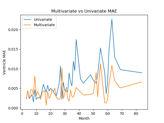
Figure 1: MAE of Ventricles over time

Our contributions are as follows:

• Incorporate model bias into deep neural networks To the best of our knowledge this is the first paper to address long-horizon forecasting problem. That is, this is the first multivariate model that captures changes over a long period of time on a large scale.

• Experiments We show that by introducing bias models outperforms all state-of-the-art models when applied to several datasets.

2 Background

2.1 LSTM

A popular choice for forecasting is Long Short-Term Memory (LSTM) (hochreiter1997long); that is because LSTMs incorporates memory units that explicitly allow the network to learn when to “forget” previous hidden states and when to update hidden states given new information. The LSTM unit shown in figure 2.

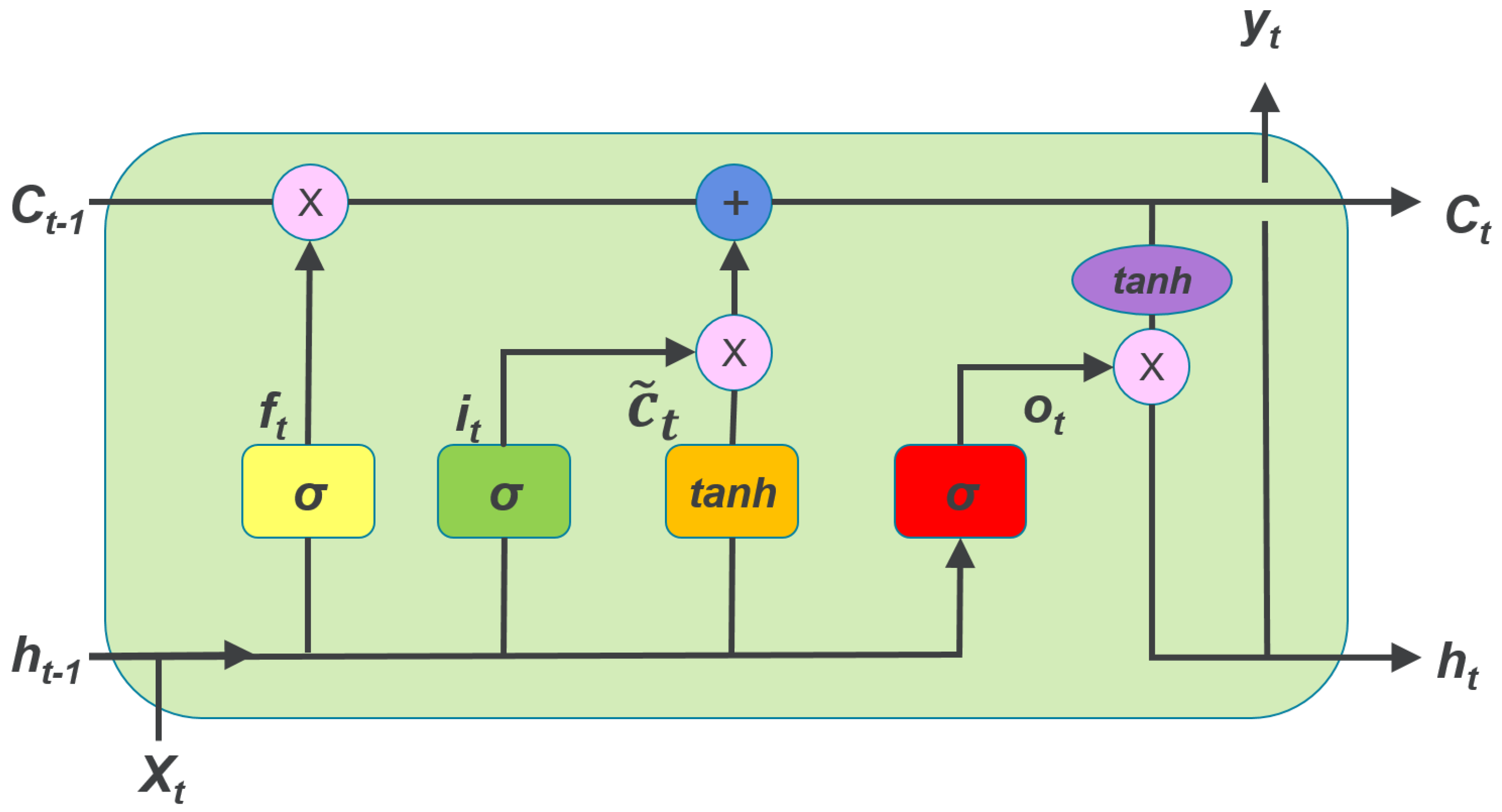
Figure 2: Long Short-term Memory Neural Network

The state updates satisfy the following operations:

$$\begin{split}&\mathbf{i}_{t}=\sigma\left(\mathbf{W}_{xi}\mathbf{x}_{t}+\mathbf{W}_{hi}\mathbf{h}_{t-1}+\mathbf{b}_{i}\right)\\ &\mathbf{f}_{t}=\sigma\left(\mathbf{W}_{xf}\mathbf{x}_{t}+\mathbf{W}_{hf}\mathbf{h}_{t-1}+\mathbf{b}_{f}\right)\\ &\mathbf{o}_{t}=\sigma\left(\mathbf{W}_{xo}\mathbf{x}_{t}+\mathbf{W}_{ho}\mathbf{h}_{t-1}+\mathbf{b}_{o}\right)\\ &\mathbf{\tilde{c_{t}}}=\tanh\left(\mathbf{W}_{xc}\mathbf{x}_{t}+\mathbf{W}_{hc}\mathbf{h}_{t-1}+\mathbf{b}_{c}\right)\\ &\mathbf{c}_{t}=\mathbf{f}_{t}\odot\mathbf{c}_{t-1}+\mathbf{i}_{t}\odot\mathbf{\tilde{c_{t}}}\\ &\mathbf{h}_{t}=\tanh\left(\mathbf{o}_{t}\odot\mathbf{c}_{t}\right)\end{split}$$ (1)

Here $\sigma$ is the logistic sigmoid function and $\odot$ is the Hadamard (element-wise) product; $\mathbf{W}_{i},\mathbf{W}_{f},\mathbf{W}_{o},\mathbf{W}_{c}$ are recurrent weight matrices; $\mathbf{b}_{i},\mathbf{b}_{f},\mathbf{b}_{o},\mathbf{b}_{c}$ are the bias terms. In addition to a hidden unit $\mathbf{h}_{t}$ , the LSTM includes an input gate $\mathbf{i}_{t}$ , forget gate $\mathbf{f}_{t}$ , output gate $\mathbf{o}_{t}$ , input modulation gate $\mathbf{\tilde{c_{t}}}$ , and memory cell $\mathbf{c}_{t}$.

Note that there is other variations of LSTM including Gated recurrent unit GRU (gru), No Forget Gate (NFG), No Peepholes (NP) , No Input Activation Function (NIAF) and others. A comparison between different variations of LSTM was done by (greff2017lstm) and there results show that although LSTM variations are computationally cheaper, none of the variants can improve upon the standard LSTM architecture significantly. Since we are proposing a general purpose long-horizon forecasting model we will use the standard LSTM shown in figure 2.

2.2 Markov chain and Maximum Likelihood

A Markov chain is a probabilistic sequence model figure 3 shows a simple Markov chain where $X:x_{1},x_{2},x_{3},...,x_{N}$ represents states, $N$ is the number of states which maybe discrete (taking values in a finite i.e diagnosis) or continuous (taking values in an uncountably infinite set i.e ventricular volume) and $a$ is the probability of transition from one state to another, Markov chain assumes that predictions for the future state is based solely on its present state. This is known as Markov Assumption (gagniuc2017markov):

$$P\left(x_{t}\mid x_{1},\ldots,x_{t-1}\right)=P\left(x_{t}\mid x_{t-1}\right)$$ (2)

Where $x_{t}$ is state $X$ at time $t$. Also in any state the sum of transition probabilities is given by:

$$\sum_{i,j=1}^{N}a_{ij}=1$$ (3)

Where $i$ is the current state.

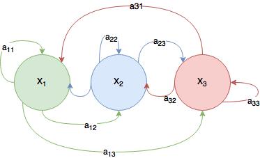
Figure 3: Markov Chain

We will be using the the concept of Markov chain to predict the changes from one observed state to another an example is the change between diagnosis (Cognitive normal, Mild cognitive impairment and Alzheimer disease).
To estimate the transition parameters $a$ we use maximum likelihood (Figueredo:2009dg), from equation 2 we can infer the following:

$$a_{ij}=P\left(x_{t}=j\mid x_{t-1}=i\right)$$ (4)

Taking a sample from the chain of size $n$ where $x^{n}_{1}\equiv x_{1},x_{2},\ldots,x_{n}$. This is a realization of the random variable $X_{1}^{n}$ we deduce the following:

$$P\left(X^{n}_{1}=x^{n}_{1}\right) =P\left(X_{1}=x_{1}\right)\prod_{t=2}^{n}P\left(X_{t}=x_{t}\mid X_{t-1}=x_{t-1}\right)$$ (5)

$$=P\left(X_{1}=x_{1}\right)\prod_{t=2}^{n}a_{x_{t-1}x_{t}}$$

$$=P\left(X_{1}=x_{1}\right)\prod_{i=1}^{k}\prod_{j=1}^{k}a_{ij}^{n_{ij}}$$

Where $n_{ij}$ is the number of times $i$ is followed by $j$ in $X^{n}_{1}$; the objective function is to maximize equation 5, taking the $\log$ gives us:

$$\log\text{L}\left(a\right) =\log P\left(X_{1}=x_{1}\right)+\sum_{ij}n_{ij}\log a_{ij}$$ (6)

Differentiating equation 6 then solving for $a$ we get the following:

$$\hat{a}_{ij} =\frac{n_{ij}}{\sum_{j=1}^{m}n_{ij}}$$ (7)

3 Models

In this work, we compare three models: a multivariate LSTM with a single target and bias as shown in figure 4 and Continuous multivariate LSTM with multiple target and bias figure 5.

3.1 Simple Multivariate LSTM with bias

In the first approach (figure 4) we use Multivariate LSTM Recurrent Neural Networks, the input to the first LSTM are actual features, for all future LSTM the input is the bias term $x_{bias_{i}}$ and the value of output from the previous LSTM. We introduce a new term $\tilde{x}_{t}$ such that:

$$\tilde{x}_{i}=\left\{\begin{array}[]{ll}x_{i}\text{ at }t=0\\ x_{bias_{i}}\text{ at }t\neq 0\end{array}\right.$$ (8)

$x_{bias_{i}}$ is the output of the bias function that will be introduced in section 3.3. Our Model looks like this:

$$y_{t+1}=\text{ LSTM}(\tilde{x}_{1t},\tilde{x}_{2t},\ldots,\tilde{x}_{nt},y_{t})$$ (9)

$n$ is the number of features and $y$ is the target/

Figure 4: Simple Multivariate LSTM with 3 features and one target

The optimization objective is to find parameters that yield measurements that are close to the actual values of the ventricular volume, i.e.

$$\text{minimize }\left(\text{ loss}\left(\hat{y},y\right)\right)$$ (10)

$\hat{y}$ is the predicted value, we use mean absolute error for loss.

3.2 Continuous Multivariate LSTM with bias

Continuous Multivariate LSTM Recurrent Neural Network (figure 5) the output of the an LSTM is the input of the next.

Figure 5: Continuous Multivariate LSTM with bias

Each feature is represented as:

$$\tilde{x}_{it}\coloneqq\left[x_{it},x_{bias_{i}}\right]$$ (11)

Where $x_{bias_{i}}$ is the output of the bias function and $x_{it}$ is feature $i$ at time step $t$. Now, we have the following model:

$$x_{1t+1},x_{2t+1},\ldots,x_{nt+1}=\text{ LSTM}(\tilde{x}_{1t},\tilde{x}_{2t},\ldots,\tilde{x}_{nt})$$ (12)

Now the new objective is to find parameters that yield measurements that are close to the actual values and the other features as well, i.e.

minimize $$\left(\sum_{i=1}^{n-1}\alpha_{i}\cdot\text{ loss}\left(\hat{x}_{i},x_{i}\right)\right)+$$ (13)

$$\left(\left(1-\sum_{i=1}^{n-1}\alpha_{i}\right)\cdot\text{ loss}\left(\hat{x}_{n},x_{n}\right)\right)$$

$\hat{x}$ is the predicted value, $x_{n}$ represents the feature of interest and $\alpha_{i}\in\left[0,1\right]$ is a hyper-parameter which indicates the importance of each feature $\sum_{i=1}^{n}\alpha_{i}=1$, we use mean absolute error for loss. At prediction time we only take the output of $x_{n}$ which is our target, all other outputs are used strictly for the future predictions.

3.3 Bias

Adding bias to account for long-term changes in the variable came from Markov chain and maximum likelihood section 2.2, if you look at the problem as a Markov chain then the forecasting goal is to find the next state that gives maximum likelihood adding bias helps increase maximum likelihood accuracy. Input to the bias function is the features $x_{1t},\ldots,x_{nt}$ and time $t$. We will compare between different bias functions introduced bellow.

3.3.1 Population Averaging

Bias is calculated using the following equation

$$x_{bias_{i}}=\beta x_{i}+\left(1-\beta\right)\mu_{i}$$ (14)

$\beta$ is a hyper-parameter $\beta\in\left[0,1\right]$ where $\beta=1$ at $t=0$ and $\beta=0$ at $t\rightarrow\infty$, here $\mu_{i}$ is the average of $x_{i}$ for all samples $N$

$$\mu_{i}=\frac{1}{N}\sum_{j=0}^{j=N}x_{ij}$$ (15)

3.3.2 Clustering

The idea group similar patients together so as time passes patient belonging to the same group get closer together, Since we have 3 diagnosis so we decided to have 3 clusters we are using K-Means algorithm (hartigan1979algorithm) with $K=3$ the euclidean distance between point $x$ and cluster center $c_{j}$ is calculated using the following equation:

$$\sum_{i=1}^{i=N}\sum_{j=1}^{j=K}||x_{i}-c_{ij}||^{2}$$ (16)

Where $i$ represents the features and $j$ is the cluster, the point is assigned to the cluster with the smallest distance. The cluster centers are calculated during training to reduce computational overhead at prediction. Once the point is assigned to a cluster the bias is calculated by

$$x_{bias_{i}}=\beta x_{i}+\left(1-\beta\right)c_{ij}$$ (17)

Where all variables are similar to equation 14 except $\mu$ is replaced with $c_{j}$ which is the assigned cluster.

4 Experiments

We show that classical LSTMs are not able to provide accurate long-term forecasts. We present both quantitative and qualitative analysis of our models and show that in most cases it does better the classical LSTM for this specific problem.

In order to study the effectiveness of model based bias on long term forecasting, We used two real-world datasets to evaluate our models both are publicly available. The first dataset is from the Alzheimer’s Disease Neuroimaging Initiative (ADNI) , this dataset was used to predict the change in ventricular volume over time, we are particularly interested in the ventricular volume since there is a link between ventricular enlargement and Alzheimer’s disease (AD) progression (nestor2008ventricular) (ott2009relationship). The second dataset is a monthly electricity consumption dataset obtained from Energy Information Administration (EIA) (outlook2008energy) and NOAA’s National Centers for Environmental Information (NCEI) (NOAA) which is used to predict the amount of electricity in Megawatt hours each state uses per month.

Details of the datasets, setup and experiments will be given in the sections bellow.

4.1 Ventricular forecasting

Data Description

We are using ADNI dataset that was used in the Tadpole challenge (tadpole), the data consists of 1628 subject which are either cognitively normal (CN), stable mild cognitive impairment, early mild cognitive impairment, late mild cognitive impairment or have Alzheimer disease. This data was collected over a 10 year period measurements were typically taken every six month, since subjects were allowed to enter and leave the trial at any point the number of visits per subject was different, figure 6 shows the number subjects that showed up at every visit.

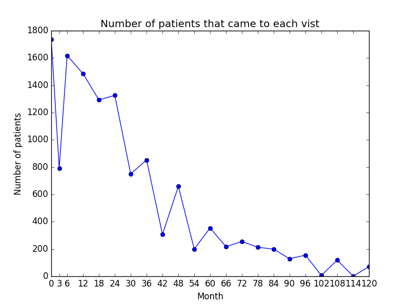
Figure 6: Number of subject that came to a visit

Data consists of 1835 features which come the following biomarkers:

• Cognitive test a neuropsychological tests administered by a clinical expert.

• MRI which measures of brain structural integrity.

• FDG Positron Emission Tomography (PET) measure cell metabolism, where cells affected by AD show reduced metabolism.

• AV45 and AV1451 PET measures a specific protein (amyloid-beta and tau respectively) load in the brain.

• Diffusion Tensor Imaging (DTI) measures microstructural parameters related to cells and axons.

• Cerebrospinal fluid (CSF) Biomarkers.

• Others including diagnosis, genetic and demographic information.

Data preparation

In order to prepare data for forecasting the following steps were followed:

• Make all observations have same amount of time between them since all visits are 6 month apart except for the second visit which is 3 month after the initial visit all data from that visit was discarded.

• Transform time series into supervised learning problem this was done by making data at time t-1 feature and at time t target.

• Transform time series into stationary data this was done by removing dependencies so the difference between observations was used instead of the the observation value.

• Feature Scaling This was done by feature standardization (wiki:xxx) which makes the values of each feature in the data have zero-mean (when subtracting the mean in the numerator) and unit-variance. The general method of calculation is to determine the distribution mean and standard deviation for each feature. Next we subtract the mean from each feature. Then we divide the values (mean is already subtracted) of each feature by its standard deviation.

• Missing data We analyzed missing data dividing them into two categories, missing at random or not missing at random for example if one exam is only done once at the first visit for all subjects then it is not missing at random in this case we insert the correct value of that exam. For data missing at random Hot Deck was used for imputation.

• Feature extraction We used a random forest (breiman2001random) to select features with highest cross entropy. The package used was the standard randomForest package in R.

Setup

The setup is similar to that of the TADPOLE Challenge (tadpole). Data was divided into two datasets, a training dataset that contains a set of measurements for every individual that has provided data to ADNI in at least two separate visits (different dates) these measurements are associated with outcomes, i.e. the targets for forecasting are known and a test dataset that contains a single (most recent) time point and a limited set of variables from each rollover individual. Individuals in the test dataset are not used when forecasting or training/building training models. The goal is to make month-by-month forecasts for normalized ventricular volume of each individual in the test dataset for a period of 5 years. Training Dataset was then divided into two sub-dataset training and validation.

For evaluation we use forecasts at the months that correspond to data acquisition. Accuracy is measured using the mean absolute error

$$\mu_{i}=\frac{1}{N}\sum_{i=0}^{i=N}|\tilde{M_{i}}-M_{i}|$$ (18)

where $N$ is the number of data points acquired by the time the forecasts are evaluated, $M_{i}$ is the actual value for that individual at that time and $\tilde{M_{i}}$ is the predicted value.

Our LSTM was implemented using TensorFlow (DBLP:journals/corr/AbadiABBCCCDDDG16). We train each LSTM for 1000 epochs using Adam: A Method for Stochastic Optimization (DBLP:journals/corr/KingmaB14). We used variable length LSTM since the number of visits per subject is not constant. Our final networks use 2 hidden layers and either 64 memory cells per layer and learning rate 0.0003. These architectures are also chosen based on validation performance.

Each model was run twice, once with regular target i.e target at time $t-1$ is value at time $t$ and the second time using sequential target replication (lee2015deeply). Since we want to teach the network to pass information across many sequence steps in order to affect the output this can be done by replicating targets at each sequence step, providing a local error signal at each step this technique was used by (lipton2015learning), figure 7 shows an unrolled LSTM with target replication each box represents a timestep the target for all timesteps is equal to that of the last timestep.

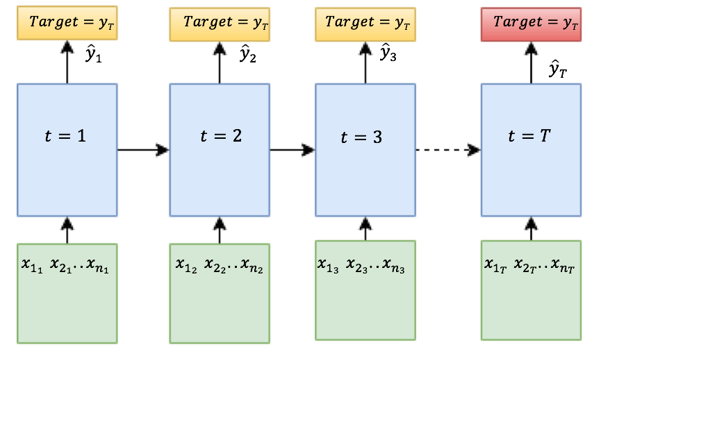
Figure 7: Single unrolled LSTM

Baseline

Persistence Alzheimer biomarkers are highly persistent overall, but many individuals became better or worse. The persistence and change in severity of an AD patient depends on many factors including initial severity, exercise and drug management. For this reason we decided to use persistence as the simplest possible baseline.

Classical univariate LSTM The LSTM takes the ventricular volume as an input its output is the predicted ventricular volume which is the input to the next LSTM shown in figure 8.

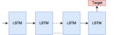
Figure 8: Univariate LSTM

Classical multivariate LSTM The LSTM takes ventricular volume along with other features as input it outputs the predicted ventricular volume, this output along with the other unchanged features is the input to the next LSTM as shown in figure 9.

Figure 9: Multivariate LSTM

Results

Figure 10 compares the performance of Model one with bias against all baselines with target replication, the figure shows that in using either averaging or K-mean bias outperforms baselines.

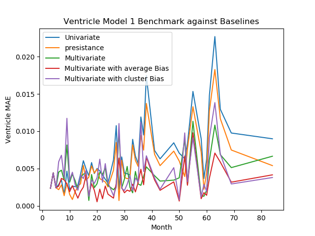
Figure 10: Ventricles MAE benchmark for Model 1 with target replication for Kmean Bias K=2

4.2 Electricity forecasting

Data Description

Electricity consumption in Megawatt Hours, population Count and price of Kilowatt Hours of electricity was obtained from Energy Information Administration (EIA) (outlook2008energy), we used data from January 2007 till October 2017 monthly for every state and the District of Columbia giving a total of 130 timesteps, average temperature of that state obtained from NOAA’s National Centers for Environmental Information (NCEI) (NOAA) was added as an additional feature, giving a total of 4 features at each month.

Data preparation

Since we did not have any missing data in this dataset we only needed to transform time series into supervised learning problem, change time series data into stationary data and preform feature Scaling. This was done using the same method described for the ventricular forecasting experiments section 4.1.

Setup

Models were trained on data from January 2007 till October 2015 and then goal is month-by-month forecasts of normalized Megawatt Hours of electricity consumed by each state from November 2015 till October 2017. Accuracy is measured using the mean absolute error given in equation 18. A shallow 2 layer LSTM with 64 memory cells per layer and learning rate of 0.0001 was trained with 500 epochs using Adam: A Method for Stochastic Optimization.

All experiments were preformed twice, first with regular target and then using sequential target replication as described in section 4.1.

Baseline

Baseline is classical multivariate LSTM as shown in figure 9.

Results

Figure 11 shows the effect of changing the number of cluster centers in K-mean algorithm on MAE for Model one, in almost all cases adding bias to the model improves the accuracy results shown here are without using target replication techniques.

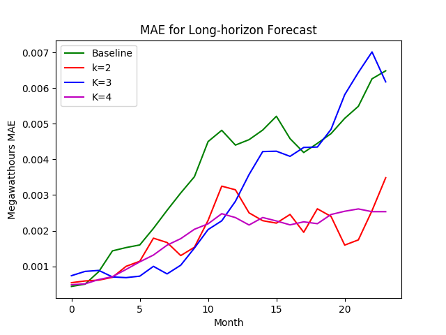
Figure 11: Studying the effect of changing the number of cluster center on accuracy

Table 1: Results Summary For ADNI Dataset

Model	Bias	Number of centers	With Target Replication	Without Target Replication
Persistence	None
Univariate LSTM	None		0.005042
Model 1	None		0.003886
Model 1	Averaging	1	0.002673
Model 1	Kmean	2	0.004237
Model 1	Kmean	3
Model 1	Kmean	4
Model 2	None
Model 2	Averaging	1
Model 2	Kmean	2
Model 2	Kmean	3
Model 2	Kmean	4

5 Conclusion and Discussion