Quantum stabilization of microcavity excitation in a coupled microcavity–half-cavity system

Abstract

We analyze the quantum dynamics of a two-level emitter in a resonant microcavity with optical feedback provided by a distant mirror (i.e., a half-cavity) with a focus on stabilizing the emitter-microcavity subsystem. Our treatment is fully carried out in the framework of cavity quantum electrodynamics. Specifically, we focus on the dynamics of a perturbed dark state of the emitter-microcavity subsystem to ascertain its stability (existence of time oscillatory solutions around the candidate state) or lack thereof. In particular, we find conditions under which multiple feedback modes of the half cavity contribute to the stability, showing certain analogies with the Lang-Kobayashi equations, which describe a laser diode subject to classical optical feedback.

I introduction

With recent advances in the fabrication of nanophotonic structures, there is an increasing ability to control and manipulate the optical properties on the single-photon level J. McKeever (1997); Lodahl et al. (2015); Reiserer and Rempe (2015). One of the techniques central to such control is the ability to access the strong-coupling regime of cavity quantum electrodynamics (cQED). In solid-state structures, recent developments include coupling quantum emitters such as quantum dots (QD) to photonic crystals Lodahl et al. (2004); Söllner et al. (2015); Nomura et al. (2009) and micropillar cavities Böckler et al. (2008); Gazzano et al. (2013). These devices provide unidirectional photons that are of interest, for example, to improve quantum communications over long distances Bouwmeester et al. (1997). In addition, the ability to control and coherently manipulate photons coupled to the internal state of the QD is of great importance due to potential applications in quantum memory and quantum information processing Giesz et al. (2016).

Controlling a quantum system–in the sense of providing stabilization of its quantum state–presents a nontrivial problem. The use of feedback to provide stabilization in classical systems is quite advanced, while less is known for quantum system. Two feedback-control schemes have been explored recently in quantum optics, viz.  measurement-based and coherent feedback loops Serafini (2012); Wiseman and Milburn (2009). In a measurement-based feedback loop, the quantum system is monitored and the outcome of the measurement is used as classical information to manipulate the operations. A measurement-based feedback loop has been implemented in a cQED system with trapped atoms Wiseman and Milburn (1993). In coherent feedback, the dynamics are entirely quantum mechanical and the system interacts coherently with an ancillary subsystem in both the extraction and manipulation processes. For coherent feedback, such as Pyragas feedback Pyragas (1992), both processes utilize information stored in the reservoir degrees of freedom residing, for example, in an external cavity (EC).

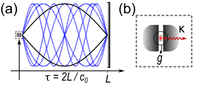
Figure 1: (a) The quantum-dot-micro-cavity system coupled to an EC of length $L$ in which a quasi-continuum of photon modes exist. $\tau$ is the delay time of the coherent feedback. The black and the blue curves indicates classical electric fields forming standing waves from the external cavity. (b) Schematic of a two-level QD in a near-resonant MC, where $g$ is the coupling strength and $\kappa=\pi G_{0}^{2}/(2c_{0})$ is the MC damping rate.

Canonical consideration

Given that the measurement process will unavoidably collapse the wavefunction, measurement-based feedback presents limitations when the target state is a superposition. To implement coherent quantum feedback in quantum optics, one typical configuration consists in coupling the quantum system with an external half-cavity, having a perfect mirror at the opposite end, as illustrated in Fig. 1(a), similar to the time-delayed feedback setup used in EC semiconductor lasers (ECSL). The dynamics of ECSLs have been intensively studied based on the semiclassical Lang-Kobayashi (LK) equations Lang and Kobayashi (1980). The LK equations describe the nonlinear dynamics of the electric-field amplitude $|E|$, carrier density $n$ in the active region, and optical phase $\Delta\phi$ by a set of equations of motions (EOM) in the form of coupled delayed-differential equations. The dynamics are described by trajectories in phase space spanned by the three dynamical variables.

The presence of time-delayed feedback is known for the ECSL to generate multiple steady-state solutions. The stable modes of the EC are called EC modes (ECM), while the unstable modes of the EC are known as antimodes Henry and Kazarinov (1986). Depending on the various parameters of the system (e.g., injection current, feedback strength, optical feedback phase $\Delta\phi$, and EC length $L$), various dynamics can occur near and amongst these solutions Wolfrum and Yanchuk (2006); Green (2010). In particular, oscillatory dynamics about various ECMs occur in certain parameter regimes, and are closely related to undamped relaxation oscillations Erneux et al. (2007), while more complex behavior exhibiting closed trajectories encircling one or more steady-state solutions are also observed. The emergence of multiple solutions is often seen in many nonlinear systems, but not in a quantum system with a finite number of degrees of freedom ECKHAUS (1965). However, in quantum systems with a bath of infinite degrees of freedom (in our case, the modes of the EC), once these are integrated out, the system may exhibit what appears to be nonlinear behavior in the remaining explicitly considered degrees of freedom.

Another point of view of nonlinearity in quantum systems with coherent feedback is to consider the variation in the dynamical behavior with the number of photons. The nonlinearity involving states with a small number of photons has been observed experimentally Hopfmann et al. (2013); Albert et al. (2011). These effects cannot be described with a classical electromagnetic field, i.e., the scaling of the behavior with photon number cannot be accounted for by the corresponding optical intensity. Hence, a fully quantum mechanical treatment of such time-delayed systems, including the electromagnetic field, is essential to understand the dynamics of single-photon emitters with coherent time-delayed feedback.

Broadly speaking, two approaches have been used to account for the coherent feedback. In one approach, the non-Markovian evolution of the coherent feedback effect is analyzed with a differential equation with a time-propagator Grimsmo (2015). On the other hand, the optical feedback from a mirror has typically been accounted for using a one-dimensional model for the electromagnetic field with a standing-wave basis in the Markovian limit Cook and Milonni (1987); Dorner and Zoller (2002); Beige et al. (2002). Recent theoretical studies have focused on Markovian coherent feedback in various systems, such as ensembles of atoms Cook and Milonni (1987); Dorner and Zoller (2002); Beige et al. (2002), a single atom in a cavity Chang et al. (2012), one-dimension waveguides Fang et al. (2015); Guimond et al. (2017); Hoi et al. (2015); Tufarelli et al. (2014); Calajó et al. (2018), and photonic crystals Carmele et al. (2013); Kabuss et al. (2015); Pichler and Zoller (2016). It has been demonstrated that the standing-wave field model in a half cavity (Markovian) is equivalent to a time-delayed feedback system (non-Markovian) Beige et al. (2002); Kabuss et al. (2015). The control of the delay time can be a key factor in the stability or instability as well as the nonlinear dynamics in many complex systems Soriano et al. (2013); Grimsmo et al. (2014), providing wide-range applications. These works provide a promising route to rapid convergence of states Grimsmo et al. (2014), enhancing entangled photon-pair generation from biexcitons Hein et al. (2014), and to drive continuous exchanges for pure states Carmele et al. (2013). Among these studies, stability in coherent feedback systems has been investigated by Grimsmo Grimsmo (2015) based on linear delayed differential equations (non-Markovian). Since then, few other studies have focused on stability and its relation to time-delayed systems Német and Parkins (2016); Tabak and Mabuchi (2016). The evolution of the quantum states in these investigations is described by means of a time-varying Hamiltonian. These works are focused on specific features of the quantum system and not on the stability of the target state, which from the standpoint of experimental realization or practical application is of key importance.

In this study, we consider a quantum system composed of a single-photon emitter in the form of a quantum dot (QD) within a microcavity (MC) formed by a micropillar with coherent quantum feedback provided by a distant mirror as shown in Fig. 1(a). Specifically, in view of the relative lack of understanding of how quantum feedback can provide stability in quantum systems, we focus on analyzing the stability of such system in various parameter spaces. Thus, this work provides a testbed to study time-delayed feedback in a fully quantum system, as well as addresses a physical implementation of such a system of interest for nanophotonic and quantum information-science applications. Our approach presents a direct stability analysis in the Markovian dynamics of quantum feedback from a single-photon emitter. The quantum feedback is achieved via the EC, similar to previous studies Carmele et al. (2013); Kabuss et al. (2015). We derive a set of EOMs for the quantum amplitudes associated with the natural basis describing the QD excitation, the MC photon, and the EC modes. The EOMs of the state vector are obtained with the input-output formalism in the Schrödinger picture instead of in the Heisenberg picture as in Ref. Pichler and Zoller (2016).

Since photon leakage from the EC is neglected, our system conserves excitation number. Our focus is on the one-excitation subspace. In the one-excitation subspace, we find the stationary-state solutions, which we then investigate for stability. By stationary state, we mean states in which the probabilities in the noninteracting basis remain constant in time even including the interaction. In other words, stationary states are those that are simultaneously eigenstates of both the noninteracting and the interacting Hamiltonians. We explore the stabilty of the stationary states, that is, states of the composite MC/QD subsystem that are effectively decoupled from the EC. We find that the stable stationary states are represented by the MC/QD and its mirrored-self being in a singlet state Vetter et al. (2016). Similar observations have been made that the singlet state corrresponds to Dicke subradiant state Dicke (1954) in a waveguide system Chang et al. (2012), in a system with chiral feedback from a single V-level atom Guimond et al. (2016). To be more specific, the singlet state would appear effectively decoupled from the waveguide, being in a dark state which is subradiant, and thus stable, whereas the triplet state is superradiant, and thus unstable, as it decays at twice the cavity damping rate from the MC, Chang et al. (2012); Guimond et al. (2016). In the case with one single-photon emitter coupled to the EC, the subradiant (dark) state would be the only stationary state where the population in QD and MC are antisymmetric Dicke (1954).

We determine the stability by studying the dynamics in the vicinity of the stationary state. This is done by constructing the Jacobian matrix of the linearized EOMs with the state amplitudes perturbed from the stationary state ECKHAUS (1965), a technique widely employed for classical stability analysis. We analyze the eigenvalues of the Jacobian matrix as a function of coupling strength between the MC and EC. A strictly imaginary eigenvalue indicates oscillatory dynamics about the candidate stationary state, which is thus deemed stable while a positive (negative) real part of the complex eigenvalues indicates unstable (stable) stationary states. The effects of time delay are also studied for various EC length $L$. We numerically verify the Jacobian analysis by perturbing the stationary state to investigate its stability, which agrees with the results obtained directly from the Jacobian of the state amplitudes.

The remainder of the paper is organized as follows. In the next section, we outline the cQED description of the system. We next find the stationary state. Following this, we assess the stationary state’s stability. In the final section, we conclude.

II Theoretical description of the single-emitter, microcavity, external cavity system

We begin by introducing the system. We consider an intrinsic QD coupled to a single near-resonant mode of a high-$Q$ micropillar MC [Fig. 1 (b)] and coupled in turn to the EC modes shown in Fig. 1(a). The QD is characterized by interband-transition frequency, $\omega_{0}$. The QD interband transition is dipole coupled to a single mode of the micropillar MC of angular frequency $\omega_{MC}$ (in this study, we will eventually take $\omega_{MC}=\omega_{0}$) with coupling strength $g$, as in Ref. Somaschi et al. (2016). This approach can yield strong coupling between the QD and the MC Hein et al. (2014) and can generate high-purity, indistinguishable single photons Somaschi et al. (2016). We place an ideal mirror with reflection coefficient $r\!=\!-1$ a distance $L\!=\!c_{0}\tau/2$ from the micropillar to form the EC (half cavity), with $c_{0}$ the speed of light in vacuum and $\tau$ the EC round-trip feedback time. The conditions we choose are similar to the single QD in a MC subjected to an external mirror in a recent paper Kabuss et al. (2015). For a mirror with $|r|\!<\!1$, the coherent feedback can be treated considering the mirror properties Faulstich et al. (2018), while analysis can be perform using an open quantum-system formalism, discussed in a recent publication by Whalem Whalen et al. (2017).

We work in the rotating-wave approximation (RWA) Walls and Milburn (2007) in the Schrödinger picture as in Refs. Cook and Milonni (1987); Carmele et al. (2013); Kabuss et al. (2015). The derivation of the interaction Hamiltonian can be found in Ref. Cook and Milonni (1987); Carmele et al. (2013); Kabuss et al. (2015); Garrison and Chiao (2008); Walls and Milburn (2007); Naumann et al. (2017); Pichler and Zoller (2016) (see supplementary material). For the EC, we use the free-space dispersion for photons, $\omega_{k}\!=\!c_{0}\absolutevalue{k}$, assuming a sufficiently large value of $L$ so that the photon modes can be considered a quasi-continuum. We assume that only the optical modes with angular frequencies near $\omega_{0}$ interact strongly with the MC photon ($\omega_{k}\!\approx\!\omega_{MC}\!\approx\!\omega_{0}$). We obtain the following interaction Hamiltonian describing the QD coupled to the MC mode and that mode in turn coupled to the EC modes,

$$\frac{H_{int}^{(RWA)}}{\hbar}\!=\!-\omega_{g}(\sigma^{-}a^{\dagger}\!+\!\sigma^{+}a)\!-\!\!\int_{-\infty}^{\infty}\!\!\!\!\!d\omega_{k}[G(k,t)a^{\dagger}b_{k}\!+\!\rm{h.c.}]$$

with $\omega_{g}=g/\hbar$, $a^{\dagger}$ ($a$) the creation (annihilation) operator for the MC photon and $\sigma^{+(-)}$ the raising (lowering) operator of the two-level QD system. The bosonic operators $b_{k}$ destroy a photon of frequency $\omega_{k}$ in the EC as defined as in Ref. Pichler and Zoller (2016) and the coupling element, $G(k,t)=G_{0}\sin(kL)e^{i(\omega_{0}-\omega_{k})t}$, where $G_{0}=\sqrt{2c_{0}\kappa/\pi}$. Note that because $H_{int}^{(RWA)}$ is quadratic in creation and annihilation operators, the Hamiltonian conserves the number of excitations. We extend the lower limit of integration to $-\infty$ given the interaction bandwidth is narrow compared with $\omega_{0}$. A detailed discussion is presented in the supplemental material.

We now concentrate on the one-excitation subspace where an arbitrary wavefunction can be written

$$\Psi(t)\!=\!c_{e}(t)\ket{e,0,0}\!+\!c_{c}(t)\ket{g,1,0}\!+\!\int_{-\infty}^{\infty}\!\!\!\!c_{k}(t)\ket{g,0,k}dk.$$

Here, in kets $\ket{a,b,k}$, $a\!=\!e$ ($g$) denotes the QD in the excited (ground) state; $b\!=\!0$ (1) denotes zero (one) MC photon; and $k$ denotes the EC photon wavevector. $\Psi(t)$ is thus described by the time-dependent amplitudes $c_{e}(t)$, $c_{c}(t)$, and $c_{k}(t)$.

III stationary state

Substituting $\Psi(t)$ into the time-dependent Schrödinger’s equation, we obtain the following coupled EOMs for the time-dependent amplitudes,

$$\frac{\partial c_{e}}{\partial t}= \;i\omega_{g}\;c_{c},$$ (3)

$$\frac{\partial c_{c}}{\partial t}= \;i\omega_{g}\;c_{e}+i\int_{-\infty}^{\infty}c_{k}~{}G(k,t)\;\mathrm{d}k,$$ (4)

$$\frac{\partial c_{k}}{\partial t}= \;iG^{*}(k,t)\;c_{c}.$$ (5)

To find the stationary states (stationary in the more narrow sense defined above), we write $c_{i}(t)=|c_{i}(t)|\exp[i\theta_{i}(t)]$, to obtain a new set of EOMs,

$$\frac{\partial c_{i}}{\partial t}=\frac{\partial\left|c_{i}\right|}{\partial t}e^{i\theta_{i}(t)}+i\frac{\partial\theta_{i}(t)}{\partial t}\left|c_{i}\right|e^{i\theta_{i}(t)},$$ (6)

with $i\!=\!e$, $c$, and $k$. We apply the constraint of stationarity $\partial\absolutevalue{c_{i}}/\partial t\!=\!0$ and find the solution as discussed in the supplemental materials.

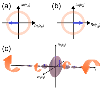
Figure 2: Representation of the one-excitation stationary state in the frame rotating at the frequency $\omega_{0}$ (a) $\bar{c}_{e}(t)$, (b) $\bar{c}_{c}(t)$, and (c) $\bar{c}_{k}(k,t)$. The blue arrows indicate the initial condition and the orange arrows indicates the time evolution.

We denote the stationary state (with respect to the interaction Hamiltonian) in the single-excitation subspace as $\bar{\Psi}(t)$ (where the bar indicates a stationary solution). In the frame rotating at $\omega_{0}$, $\bar{\Psi}_{RWA}(t)=\bar{\Psi}(t)e^{-i\omega_{0}t}$

$$\bar{\Psi}_{RWA}(t)=\bar{c}_{e}(t)\ket{e,0,0}+ \;\bar{c}_{c}(t)\ket{g,1,0}$$

$$+ \int_{-\infty}^{\infty}\bar{c}_{k}(t)\ket{g,0,k}dk.$$

We thus obtain the noninteracting amplitudes for the stationary state

$$\bar{c}_{e}(t) =-\alpha e^{-i\omega_{g}t},$$ (7)

$$\bar{c}_{c}(t) =\alpha e^{-i\omega_{g}t},$$ (8)

$$\bar{c}_{k}(k,t) =\frac{\alpha G_{0}\sin(kL)}{\omega_{k}-\omega_{g}-\omega_{0}}e^{i(\omega_{k}-\omega_{g}-\omega_{0})t}.$$ (9)

Note that the strict commensurability condition, i.e., $2L/c_{0}\!=n\;\cdot\;\!2\pi/\omega_{g}$ with $n\in\mathbb{N}$, is required for the stationary state. Detailed reasons will be explained later in this work and can also be found in Ref. Fang et al. (2015); Kabuss et al. (2015). The parameter $\alpha$ is defined in the next paragraph. Note that the minus sign results from the MC/QD being in a singlet state (antisymmetric) of the quantum system and its mirrored self Chang et al. (2012); Vetter et al. (2016); Guimond et al. (2016); Beige et al. (2002). In this state, the QD-MC subsystem are effectively decoupled from the EC, thus being in a dark or subradiant state, as discussed for similar systems in Refs. Chang et al. (2012); Guimond et al. (2016); Vetter et al. (2016).

The noninteracting amplitudes associated with this stationary state can be characterized by a single parameter

$$\alpha\!=\!\left|c_{c}(t)\right|\!=\!\left|c_{e}(t)\right|\!=\!\left(2+\frac{\pi G_{0}^{2}L}{c_{0}^{2}}\right)^{\!\!-1/2}\!=\!(2+\tau\kappa)^{-1/2}$$

where recall $G_{0}=\sqrt{2c_{0}\kappa/\pi}$ and $\kappa$ is the MC photon damping rate. Since we consider 100 % reflection from the distant mirror, the damping rate characterizes both the rate into the EC and the feedback rate from the reflected photon.

The stationary state is indicated in the frame rotating at $\omega_{0}$ in Fig. 2. The blue arrow shows the state of the QD at a snapshot in time with the time evolution in the RWA shown by the orange arrows where we choose initial conditions $\bar{c}_{e}(0)\!=\!\alpha$, $\bar{c}_{c}(0)\!=\!-\alpha$, and $\bar{c}_{k}(k,0)\!=\!\alpha G_{0}\sin(kL)/(\omega_{k}-\omega_{g})$. In this case, the EC photon is in a standing wave and its population is described by a sinc function in the $k$ channel (of frequency $\omega_{k}$), centered on $\omega_{k}=\omega_{g}$, i.e. $kL=n\pi$, with $n$ an integer number such that the commensurability condition is fulfilled : commensurability condition $\tau=n\tau_{g}$ with $\tau_{g}=2\pi/\omega_{g}$, the time it takes for the strongly-coupled exciton-photon system to perform a full Rabi oscillation. Note that each EC state, $c_{k}$, revolves around the $k$ axis at different rate, as illustrated in Fig. 2(c).

The evolution of the MC photon population $\absolutevalue{c_{c}(t)}^{2}$ is plotted in Fig. 3. The theoretical and numerical results for the stationary state just found are plotted in the black and yellow dotted curves, respectively. In this case, the MC photon population remains constant in time. The green curve (Case II) plots the MC photon population $\absolutevalue{c_{c}}^{2}$, however, for the initial state $c_{e}(0)\!=\!1$, $c_{c}(0)\!=\!0$, $c_{k}(0)\!=\!0$ for all $k$. In this case, the MC photon population varies significantly at fist and eventually mainly leaks out into the EC. Note that there is only one stationary state in our sense within the one-excitation subspace.

To lend insight into the nature of the stationary state, the initial state amplitudes of the EC photons of wavenumber, $\bar{c}_{k}(k,0)$ are given by an even function, centered on $\omega_{k}=\omega_{g}$, i.e. $kL=n\pi$ as in Fig. 2(c) and the coupling $G(k,t)=\sqrt{2c_{0}\kappa/\pi}\sin(kL)\exp[i(\omega_{0}-\omega_{k})t]$ is an odd function centered on $\omega_{k}=\omega_{g}$. Thus, while $L$ satisfies the commensurability condition, i.e., $2L/c_{0}\!=\!2\pi n/\omega_{g}$ with $n\in\mathbb{N}$, the EC is in effect decoupled from the MC photon and the QD for the stationary state. As this occurs, the QD and the MC photon experience a cavity-assisted interaction at the rate of $\omega_{g}$, and both QD and MC-photon state are stationary when their complex amplitudes are $\pi$ out of phase. The only stationary state corresponding to the interaction Hamiltonian is antisymmetric in the amplitudes $c_{e}$ and $c_{c}$, and similar to the bound state in Ref. Fang et al. (2015); Calajó et al. (2018); Tufarelli et al. (2014) or the subradiant/dark state in the recent studies of Refs. Stannigel et al. (2012); Guimond et al. (2016).

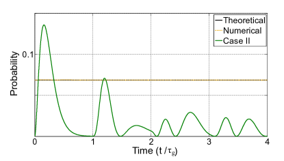
Figure 3: Time evolution of the probabilities of $\absolutevalue{c_{c}(t)}^{2}$ for various initial conditions. The QD is initialized in the excited state for the green curve (Case II); however, choosing initial conditions corresponding to a stationary state results in $\absolutevalue{c_{c}(t)}^{2}$ being independent of time (black and dotted yellow curves).

IV Stability analysis

In the previous section we identified a stationary state in the one-excitation subspace. In this section, we ascertain the stationary state’s stability, which depends on three important parameters. The first parameter is $n$, related to $\omega_{g}$ and to the EC round trip time $\tau$ through the commensurability condition $\tau=n\tau_{g}$. The second one is the ratio $R=\kappa/4g$, between the cavity damping rate, $\kappa$ and the coupling strength $g$. A third one is the feedback phase from the reflected photon after a round trip in the external cavity, $\Delta\phi=(4\pi L/\Lambda_{0}\mod{2\pi})-\pi$. The reflected photon is assumed to undergo $\pi$ phase change from an ideal mirror ($r=-1$ in this study). We note that the exact value of $\omega_{0}$ plays a role in the system behavior only through this feedback phase, as $\omega_{0}\tau=\Delta\phi+\pi\mathrm{\mod}2\pi.$

To begin, we constructed a Markovian model to numerically simulate the evolution based on Eqs. (3)-(5), and the stationarity of $\bar{\Psi}$ is demonstrated in Fig. 3. For example, for $c_{e}(0)\!=\!1$, $c_{c}(0)\!=\!0$, and $c_{k}(0)\!=\!0$ for all $k$, the MC-photon population exhibits nonperiodic oscillations on the timescale of vacuum-field Rabi oscillations, shown in Ref. Hein et al. (2014).

Next, we study the dynamics in the vicinity of the stationary state to ascertain its stability. We expect that for a stable state, the probabilities will remain near the initial values. Here, we perturb the stationary state and track the dynamics. (This numerical approach is infeasible rigorously to determine the stability of the candidate stationary state due to the existence of numerous degrees of freedom that would have to be perturbed individually; indeed, this is in effect what the method below of computing the eigenvalues of the Jacobian does for us.) We add small values $\delta_{c,i}$ to the initial conditions for $c_{e}$ and $c_{c}$ with respect to the stationary state $\bar{\Psi}(t)$ in Eqs. (6)-(8), viz. $\delta c_{c}\!=\![\pm~{}0.01,\pm~{}0.02]\alpha$ while the amplitude of QD state $c_{e}(0)$ is perturbed such that $\absolutevalue{\bar{c}_{e}+\delta c_{e}}^{2}+\absolutevalue{\bar{c}_{c}+\delta c_{c}}^{2}=\absolutevalue{\bar{c}_{e}}^{2}+\absolutevalue{\bar{c}_{c}}^{2}$. We shall see that the nature of the stable state depends crucially on the ratio $R\!=\!\kappa/(4g)$ between the MC damping rate $\kappa$ and the coupling strength $g$, the inversion of the conventional coupling strength parameter between a two-level system and a cavity, where $R<1$ ($R>1$) indicates the strong- (weak-) coupling regime Andreani et al. (1999). Small $R$ thus means the vacuum-field Rabi frequency is much larger than the MC photon leakage rate; large $R$ indicates a relatively high MC photon leakage rate compared with the vacuum-field Rabi frequency. The effect on the stability is illustrated by plotting the probability for $R\!=\!0.5$ and $R\!=\!8$. The probabilities of the excited QD state, $\absolutevalue{c_{e}(t)}^{2}$ are plotted in Fig. 4(a1) and (b1) and MC photon state $|c_{c}(t)|^{2}$ in Fig. 4(a2) and (b2) for $R\!=\!0.5,$ and $8$, respectively. Here, the feedback phase is $\Delta\phi=0$ and $n=1$ in Fig. 3 and all cases in Fig. 4.

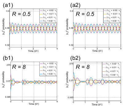
Figure 4: The evolution $\absolutevalue{c_{e}(t)}^{2}$ and $\absolutevalue{c_{c}(t)}^{2}$ of perturbed stationary states with various values of $R$. Note that the various probabilities remain near the initial values, indicating likely stability.

In Fig. 4(a1) and (a2), for small $R$ (strong coupling), the variation of the probability from its mean value exhibits oscillations at roughly the vacuum-field Rabi frequency $2\omega_{g}$ with some initial damping from $t\!=\!0$ to $\tau$ at rate $2\kappa$. For $t\!\gtrsim\!\tau$, the damping is arrested and oscillations at the vacuum-field Rabi frequency persist. By comparison, for $R\!=\!8$ [Fig. 4(b1) and (b2)] when vacuum-field Rabi oscillations do not have a chance to occur before photon leakage from the MC, the dynamics of both probabilities are not evidently periodic, indicating the participation of multiple frequencies. We shall see this is due to the participation of many coupled EC-like modes.

In order to explore the stability of the stationary state in a rigorous fashion, we consider an analysis of the eigenvalues of the Jacobian matrix Krauskopf (2000) to confirm the foregoing numerical simulations. The Jacobian is defined as the matrix of all first-order partial derivatives with respect to the each variable (in this case, the perturbed state amplitudes) evaluated for the stationary state ECKHAUS (1965). In other words, the Jacobian probes the change in the stationary state with respect to an arbitrary infinitesimal perturbation. Its eigenvalues, therefore, indicate whether or not the state is stable, with a tendency to oscillate around the stationary state for eigenvalues being strictly imaginary, stable and evolve toward a stationary state for real parts of all eigenvalues being negative, or unstable and to evolve away from the stationary state (all real parts of any complex eigenvalues being positive). In addition, saddle points are also possible where the stationary state is stable against perturbations in certain directions in state space, but not in others.

More specifically, the Jacobian matrix $\bm{J_{\delta}}$ (see supplementary materials for definition) satisfies the equation

$$\frac{\partial}{\partial t}\delta c_{i}(t)=\bm{J_{\delta}}\delta c_{i}(t).$$ (10)

We begin by studying the Jacobian matrix constructed with linearized EOMs of the perturbed state. The perturbed states along the $i$ direction in state space from the stationary state will evolve according to $\delta c_{i}(t)=\delta c_{i}(0)e^{\lambda_{i}t}$ where $\lambda_{i}$ is the eigenvalue along the $i$ direction and $\delta c_{i}(t)$ is the small perturbation along the $i$ vector from the stationary state, $\bar{c}_{\alpha}$ at $t=0$. Given the eigenvalues, possible cases for the steady state are are attractors, repellors, or saddle points corresponding to all negative, all positive, or some positive and some negative eigenvalue, respectively. The dynamics can be analyzed by the nature of the equilibrium state, in this case, the stationary state, $\bar{\Psi}(t)$ in Eqs. (7)-(9).

The interaction of the perturbed state amplitudes can be derived using linearized EOMs near the stationary state, and the Jacobian matrix of rank $(2+N)$ is derived following the small-signal model, where $N$ is the number of EC photon states, $c_{k}$, used in the simulation. Note that Jacobian, $\bm{J_{\delta}}$, is derived from linearization at the stationary state and is found to be a rank-$N+2$ skew Hermitian matrix, while the interaction Hamiltonian is a rank-2 Hermitian matrix in the one-excitation subspace.

We proceed to analyze the stability of the stationary state by considering the eigenvalues, $\lambda_{i}$s, of $\bm{J_{\delta}}$. We focus on the dependence of the eigenvalues of $\bm{J_{\delta}}$ on the ratio $R\!=\!4\kappa/g$ between the MC photon damping rate and the QD-MC coupling strength. In addition, we carry out this analysis adjusting two parameters, viz. the optical feedback phase $\Delta\phi$ and the EC round-trip time $\tau$. We first consider the effect of $\Delta\phi$, under conditions of constructive, destructive, and partial interference, and next consider the effect of varying $\tau$, restricting its value to integer multiples of $\tau_{g}=\!2\pi/\omega_{g}$, i.e., $\tau=2L/c_{0}\!=\!n\tau_{g}$ where $n\in\mathbb{\mathbb{N}}$.

In the above-mentioned scenarios, we find all the eigenvalues are purely imaginary ($i\lambda_{i}\in\mathbb{R}$). Imaginary eigenvalues indicate oscillatory dynamics upon perturbation about the stationary state, i.e., this indicates stability. Notably, since the perturbation of the stationary state evolves following $\delta c_{c}(t)=\delta c_{c}(0)\exp(\lambda_{c}t)$, we expect to observe oscillation in the probabilities both for the QD excited state and for the MC photon $\absolutevalue{c_{c}(t)}^{2}=\alpha^{2}+2\alpha\delta c_{c}(0)\cos\omega_{\rm osc}t+\absolutevalue{\delta c_{c}(0)}^{2}$, where $\omega_{\rm osc}(\lambda)=\omega_{0}+\omega_{g}-i\lambda_{c}$. The eigenvalues of the Jacobian are solutions of the determinental equation $|\bm{J_{\delta}}-\lambda\mathrm{I_{(2+N_{k})}}|=0$. One finds

$$(\omega_{\rm osc}-\omega_{g})^{2}-\kappa(\omega_{\rm osc}-\omega_{g})\sin(\omega_{\rm osc}\tau-\Delta\phi)-\omega_{g}^{2}=0.$$ (11)

Note the relationship $\omega_{0}\tau=\Delta\phi+\pi\mathrm{\mod}2\pi$ is applied in the transformation, accounting for the optical phase and the round-trip delay time. Where detailed derivation is presented in the Appendix C section.

Here, we focus on finding the frequency $\omega_{\rm osc}(\lambda_{c})$ as a function of the parameter $R=\kappa/(4g)$, the feedback phase $\Delta\phi$ (obtained by varying $L$ on the lengthscale of the photon wavelength $\Lambda_{0}=2\pi c_{0}/\omega_{0}$) of the reflected photon, and and the time delay $\tau$. Given the wide range of $R$ investigated, the following results are plotted using a horizontal scale in $\log_{2}R$.

Constructive interference: $\Delta\phi\!=\!0$. The EC round-trip distance is a half-integer multiple of the photon wavelength, $2L\!=\!(m+1/2)\Lambda_{0}$. For $R$ less than a critical value $\bar{R}(n,\Delta\phi)$ (depending on $\Delta\phi$ and $\tau$), we find only one non-zero imaginary eigenvalue and it corresponds to oscillatory dynamics about the stationary state (i.e., stability) at frequency $2\omega_{g}$. In this region, starting with perturbed initial conditions results in limit-cycle dynamics. An arbitrary perturbation leads to oscillatory dynamics at the Rabi frequency. For values of $R>\bar{R}(n,\Delta\phi)$, we find multiple emerging imaginary eigenvalues as we increase $R$. In this region, for large $L$ we have in effect a quasi-continuum of EC modes, and an arbitrary perturbation leads to non-oscillatory dynamics involving the many frequencies associated with the various eigenvalues of the Jacobian. This is a region of asymptotic stability. Recall that $n$ is the ratio of the EC round-trip time $\tau$ and the Rabi period $\tau_{g}=2\pi/\omega_{g}$. $\bar{R}(n,\Delta\phi)$ is indicated by the vertical dotted red line in Figs. 5 and 6. In the case of constructive interference, for $R=\bar{R}(1,0)\!=\!0.156$ ($\log_{2}R=-2.68$) as shown in Fig. 5(a), we find six solutions, indicating a possible bifurcating point in the strong-coupling regime. We also find that additional oscillatory modes emerge pairwise and their eigenfrequencies are smooth functions of $R$ satisfying Eq. (11). In addition, the frequency separation between the additional eigenvalues in the weak-coupling regime e.g. $R\!=\!64$ ($\log_{2}R=6$), tends toward $\delta f_{\rm osc}=1/(2\tau)$, the EC free spectral range. The expected oscillation frequencies for $n=1$ as a function of $R$ are shown in Fig. 5(a).

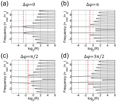
Figure 5: Frequencies of oscillation $\omega_{\rm osc}$ about the stationary state of the probability $\absolutevalue{c_{c}(t)}^{2}$ as a function of $\log_{2}R$ for various $\Delta\phi$, while n=1. The frequency is obtained from $\omega_{\rm osc}=\omega_{g}+\omega_{0}-i\lambda$, where $\lambda$ is strictly imaginary.

Destructive interference: $\Delta\phi\!=\!\pi$. The EC round-trip distance is an integer multiple of the photon wavelength, $2L\!=\!m\Lambda_{0}$. The reflected photon interferes destructively with the emitted photon at the MC. We plot the oscillation frequencies as a function of $\log_{2}R$ in Fig. 5(b) for $n=1$. Additional eigenvalues appear for $R$ above a different critical value $\bar{R}(1,\pi)\!=\!0.62$ ($\log_{2}\bar{R}(1,\pi)=-0.69$, lower than that for the case of constructive interference) as shown in Fig. 5(b). For $R$ increasing above $0.62$, two pairs of oscillating modes emerge (in addition to the existing solutions, $\omega_{\rm osc}=0$ and $2\omega_{g}$). The higher-frequency pair of eigenvalues emerges at approximately $-i(\omega_{0}+\omega_{g})+i2.75\omega_{g}$, and further splits into values separated by the EC free spectral range for higher values of $R$ (weaker coupling strength). Note that in both cases of constructive and destructive interference, the additional solutions for the frequency, $\omega_{\rm osc}$, appear symmetrically with respect to the $\omega_{\rm osc}=\omega_{g}$ axis from Eq. (11).

Partial interference: $\Delta\phi\!\neq\!0\!\neq\!\pi$. In this case, the reflected photon partially interferes with the emitted photon. The oscillation frequency of the MC photon state probability, $\omega_{\rm osc}$ depends also on the phase difference of the reflected photon. We plot the MC oscillation frequencies, $\omega_{\rm osc}$ for $\Delta\phi\!=\!\pi/2$ and $3\pi/2$ in Fig. 5(c) and (d), respectively.

An analogy exists between the behavior of the perturbed dynamics about the stationary state in the quantum system under consideration and the nonlinear dynamics of the ECSL. Under weak feedback, the LK equations predict the ECSL dynamics are strongly influenced by the optical feedback phase. Namely, it is indicated in Ref. Lenstra et al. (1984) that the laser line does not split under the influence of out-of-phase feedback, but does alternately narrow and broaden depending on the phase of the feedback. Since weak feedback in the ECSL is analogous to $R>\bar{R}$ in the quantum system, we comment here on the optical phase of the feedback field. Specifically, the feedback phase of a single photon has a similar impact on the dynamics in the weak coupling regime for the MC/QD/EC system. These effective changes appear near $R$ slightly above different critical values of $\bar{R}$ under the various interference conditions shown in Fig. 5(a)-(d).

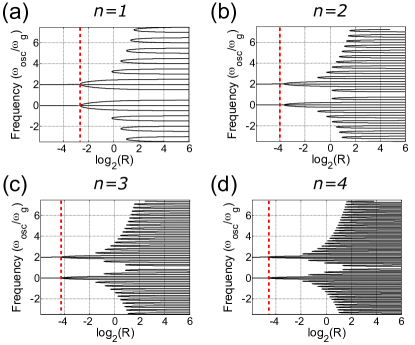
Figure 6: Frequencies of oscillation $\omega_{\rm osc}$ about the stationary state of the probability $\absolutevalue{c_{c}(t)}^{2}$ as a function of $\log_{2}R$ for various $\tau_{g}$ in the case where the feedback phase, $\Delta\phi=0$. The frequency is obtained from $\omega_{\rm osc}=\omega_{g}+\omega_{0}-i\lambda$.

We next explore the stability dependence on $R$ for various $L$. We find the stationary state only exists when commensurability condition is satisfied, i.e., the time delay, $\tau=n\;\tau_{g}$, is an integer multiple of $\tau_{g}$ where $\tau_{g}\!=\!2\pi/\omega_{g}$, and $n\in\mathbb{N}$. We chose $\Delta\phi\!=\!0$ in all cases in Fig. 6.

In the case of coherent quantum feedback from a single photon, one can show that the product of the time delay $\tau$ and the dimensionless ratio $\bar{R}(n,0)$ is constant $1/(2\pi)$ for $n\in\mathbb{N}$ from Eq. (11). We find the critical value $\bar{R}$ of $R$, beyond which more than two (imaginary) eigenvalues of the Jacobian matrix appear decreases as $L$ increases shown by various vertical dotted red lines in the panels of Fig. 6. That is, $\bar{R}(1,0)=0.16$ [$\log_{2}\bar{R}(1,0)=-2.74$], $\bar{R}(2,0)=0.08$ [$\log_{2}\bar{R}(2,0)=-3.64$], $\bar{R}(3,0)=0.053$ [$\log_{2}\bar{R}(3,0)=-4.24$], and $\bar{R}(4,0)=0.039$ [$\log_{2}\bar{R}(4,0)=-4.68$].

In the LK model for an ECSL, this product is also proportional to the dimensionless parameter $C=\gamma\tau$ characterizing feedback strength defined in Ref. Lenstra et al. (1984), where $\gamma$ is the feedback parameter. Specifically, in the theoretical study of weak optical feedback (classical ECSL), $C<1$ there is always one stable solution; for $C>1$ there may exist more stable solutions corresponds to single-frequency operation Lenstra et al. (1984). The frequency difference between the multiple solution of $\omega_{\rm osc}$ scales linearly with $n$ as one expected from the LK model. As we pointed out in the previous paragraph, the critical value, $\bar{R}$ in the single-photon limit corresponds up to a constant multiplicative factor to the feedback parameter, $\gamma$ in the classical regime. That is, $\bar{R}$ satisfies the relationship $n\bar{R}=1/(2\pi)$ ($\tau\bar{R}=\tau_{g}/(2\pi)$), represents the feedback parameter in the single photon regime.

V Discussion and conclusion

The implementation of coherence feedback with few-excitation states incorporating cQED systems can be realized in various ways. Albert, et al., have realized coherent optical feedback with microlaser, where chaotic behavior is observed with self-feedback for a few few photons $\sim 100$, and studied the second-order autocorrelation function $g^{(2)}(\tau)$ Albert et al. (2011). Note that in these experiments, more realistic parameters, including the QD dephasing rate, the QD decay rate, the transmission and reflection coefficients of the EC mirror and the MC-EC coupling are needed. However, these parameters describe the loss channels and contribute to decay of the probabilities, we expect these parameters will weakly influence the oscillation frequencies provided the large $R$ limit can be reached.

A stability analysis of the type implemented here can also be applied to the dark state existing in a quantum dimer system with a coupled cavity Stannigel et al. (2012); Guimond et al. (2016) or in certain spin systems Ramos et al. (2016); Pichler et al. (2015). In the case with spin system, the coupling element between two interacting spins placed at distance $L$ apart is replaced by $G_{sd}(k^{\prime},t)=G_{0}\cos(k^{\prime}L)e^{i(\omega_{0}-\omega_{k})t}$ Ramos et al. (2016). By making the transformation $k^{\prime}=k-\pi/2$, we obtain the relationship between the eigenvalues in two cases, i.e., the eigenvalues of $\lambda_{sd}=\lambda-\pi/2$. Following the derivation of this work, we can solve the emergent behavior of the additional solutions of $\omega_{osc,sd}(R,\Delta\phi,n)=\omega_{\rm osc}(R,\Delta\phi-\pi/2,n)$ near the stationary (dark) state. Thus, the dynamical behaviors of the interacting quantum dimer coupled through (single) photon bath should behave similarly to coherent quantum feedback. In this case, the frequencies appearing in Fig. 5 (a) and (b) must be interchanged as well as those appearing in Fig. 5 (c) and (d).

In conclusion, we consider a system composed of a QD in a MC coupled to a EC and find a stationary state where the state initialized in the MC and QD degrees of freedom is stable against decay into EC photons. Specifically, we give the analytical expression for the stationary solution for such a system in the one-excitation subspace. We find this state is stable by performing stability analysis on the Jacobian of state amplitudes. The periodic solutions perturbed about the stationary state, obtained from the eigenvalues of Jacobian, indicate additional solutions arise above a critical value $\bar{R}$ or $R$ as experimental parameters such as the cavity damping rate, the cavity coupling strength, the feedback phase, and the external cavity length are varied. We found a strong similarity to the LK model in this behavior in terms of its dependence on $\Delta\phi$ and $\tau$. In addition, numerical simulation verifies these results, showing interesting dynamics appear in the vicinity of the stationary states. Our stability analysis may serve as a bridge between classical and quantum models for nanophotonic structures subject to optical feedback.

VI Acknowledgment

We thank Dr. Yao-Lung L. Fang, and Prof. Pascale Senellart for useful discussions. The authors gratefully acknowledge the financial support of the 2015 Technologies Incubation scholarship for Dr. C. Y. Chang from Ministry of Education, Taiwan.

References

References

- J. McKeever (1997) A. D. B. J. R. B. . H. J. K. J. McKeever, A. Boca, Nature 425, 268 (1997).
- Lodahl et al. (2015) P. Lodahl, S. Mahmoodian, and S. Stobbe, Reviews of Modern Physics 87, 347 (2015).
- Reiserer and Rempe (2015) A. Reiserer and G. Rempe, Reviews of Modern Physics 87, 1379 (2015).
- Lodahl et al. (2004) P. Lodahl, A. F. Van Driel, I. S. Nikolaev, A. Irman, et al., Nature 430, 654 (2004).
- Söllner et al. (2015) I. Söllner, S. Mahmoodian, S. L. Hansen, L. Midolo, A. Javadi, G. Kiršanskė, T. Pregnolato, H. El-Ella, E. H. Lee, J. D. Song, et al., Nature nanotechnology 10, 775 (2015).
- Nomura et al. (2009) M. Nomura, N. Kumagai, S. Iwamoto, Y. Ota, and Y. Arakawa, arXiv preprint arXiv:0905.3063 (2009).
- Böckler et al. (2008) C. Böckler, S. Reitzenstein, C. Kistner, R. Debusmann, A. Löffler, T. Kida, S. Höfling, A. Forchel, L. Grenouillet, J. Claudon, et al., Applied Physics Letters 92, 091107 (2008).
- Gazzano et al. (2013) O. Gazzano, S. M. de Vasconcellos, C. Arnold, A. Nowak, E. Galopin, I. Sagnes, L. Lanco, A. Lemaître, and P. Senellart, Nature communications 4, 1425 (2013).
- Bouwmeester et al. (1997) D. Bouwmeester, J.-W. Pan, K. Mattle, M. Eibl, H. Weinfurter, and A. Zeilinger, Nature 390, 575 (1997).
- Giesz et al. (2016) V. Giesz, N. Somaschi, G. Hornecker, T. Grange, B. Reznychenko, L. De Santis, J. Demory, C. Gomez, I. Sagnes, A. Lemaître, et al., Nature communications 7 (2016).
- Serafini (2012) A. Serafini, ISRN Optics 2012 (2012).
- Wiseman and Milburn (2009) H. M. Wiseman and G. J. Milburn, Quantum measurement and control (Cambridge university press, 2009).
- Wiseman and Milburn (1993) H. M. Wiseman and G. J. Milburn, Phys. Rev. Lett. 70, 548 (1993).
- Pyragas (1992) K. Pyragas, Physics Letters A 170, 421 (1992).
- Lang and Kobayashi (1980) R. Lang and K. Kobayashi, IEEE Journal of Quantum Electronics 16, 347 (1980).
- Henry and Kazarinov (1986) C. Henry and R. Kazarinov, IEEE Journal of Quantum Electronics 22, 294 (1986).
- Wolfrum and Yanchuk (2006) M. Wolfrum and S. Yanchuk, Physical review letters 96, 220201 (2006).
- Green (2010) K. Green, Journal of Computational and Applied Mathematics 233, 2405 (2010).
- Erneux et al. (2007) T. Erneux, E. A. Viktorov, and P. Mandel, Phys. Rev. A 76, 023819 (2007).
- ECKHAUS (1965) W. ECKHAUS, NEW YORK, SPRINGER-VERLAG, INC., 1965. 117 P (1965).
- Hopfmann et al. (2013) C. Hopfmann, F. Albert, C. Schneider, S. Höfling, M. Kamp, A. Forchel, I. Kanter, and S. Reitzenstein, New Journal of Physics 15, 025030 (2013).
- Albert et al. (2011) F. Albert, C. Hopfmann, S. Reitzenstein, C. Schneider, S. Höfling, L. Worschech, M. Kamp, W. Kinzel, A. Forchel, and I. Kanter, Nature communications 2, 366 (2011).
- Grimsmo (2015) A. L. Grimsmo, Physical review letters 115, 060402 (2015).
- Cook and Milonni (1987) R. J. Cook and P. W. Milonni, Phys. Rev. A 35, 5081 (1987).
- Dorner and Zoller (2002) U. Dorner and P. Zoller, Phys. Rev. A 66, 023816 (2002).
- Beige et al. (2002) A. Beige, J. Pachos, and H. Walther, Phys. Rev. A 66, 063801 (2002).
- Chang et al. (2012) D. E. Chang, L. Jiang, A. Gorshkov, and H. Kimble, New Journal of Physics 14, 063003 (2012).
- Fang et al. (2015) Y.-L. L. Fang, H. U. Baranger, et al., Physical Review A 91, 053845 (2015).
- Guimond et al. (2017) P.-O. Guimond, M. Pletyukhov, H. Pichler, and P. Zoller, Quantum Science and Technology (2017).
- Hoi et al. (2015) I.-C. Hoi, A. Kockum, L. Tornberg, A. Pourkabirian, G. Johansson, P. Delsing, and C. Wilson, Nature Physics (2015).
- Tufarelli et al. (2014) T. Tufarelli, M. S. Kim, and F. Ciccarello, Phys. Rev. A 90, 012113 (2014).
- Calajó et al. (2018) G. Calajó, Y. Y. L. Fang, H. U. Baranger, and F. Ciccarello, arXiv preprint arXiv:1811.02582 (2018).
- Carmele et al. (2013) A. Carmele, J. Kabuss, F. Schulze, S. Reitzenstein, and A. Knorr, Phys. Rev. Lett. 110, 013601 (2013).
- Kabuss et al. (2015) J. Kabuss, D. O. Krimer, S. Rotter, K. Stannigel, A. Knorr, and A. Carmele, Phys. Rev. A 92, 053801 (2015).
- Pichler and Zoller (2016) H. Pichler and P. Zoller, Physical review letters 116, 093601 (2016).
- Soriano et al. (2013) M. C. Soriano, J. García-Ojalvo, C. R. Mirasso, and I. Fischer, Rev. Mod. Phys. 85, 421 (2013).
- Grimsmo et al. (2014) A. L. Grimsmo, A. Parkins, and B. Skagerstam, New Journal of Physics 16, 065004 (2014).
- Hein et al. (2014) S. M. Hein, F. Schulze, A. Carmele, and A. Knorr, Phys. Rev. Lett. 113, 027401 (2014).
- Német and Parkins (2016) N. Német and S. Parkins, Phys. Rev. A 94, 023809 (2016).
- Tabak and Mabuchi (2016) G. Tabak and H. Mabuchi, EPJ Quantum Technology 3, 3 (2016).
- Vetter et al. (2016) P. A. Vetter, L. Wang, D.-W. Wang, and M. O. Scully, Physica Scripta 91, 023007 (2016).
- Dicke (1954) R. H. Dicke, Phys. Rev. 93, 99 (1954).
- Guimond et al. (2016) P.-O. Guimond, H. Pichler, A. Rauschenbeutel, and P. Zoller, Phys. Rev. A 94, 033829 (2016).
- Somaschi et al. (2016) N. Somaschi, V. Giesz, L. De Santis, J. Loredo, M. P. Almeida, G. Hornecker, S. L. Portalupi, T. Grange, C. Antón, J. Demory, et al., Nature Photonics 10, 340 (2016).
- Faulstich et al. (2018) F. M. Faulstich, M. Kraft, and A. Carmele, J. Mod. Opt. 65, 1323 (2018).
- Whalen et al. (2017) S. J. Whalen, A. Grimsmo, and H. Carmichael, Quantum Sci. Technol. 2, 044008 (2017).
- Walls and Milburn (2007) D. F. Walls and G. J. Milburn, Quantum optics (Springer Science & Business Media, 2007).
- Garrison and Chiao (2008) J. C. Garrison and R. Y. Chiao, Quantum Optics (Oxford Univ. Pr., 2008).
- Naumann et al. (2017) N. L. Naumann, S. M. Hein, M. Kraft, A. Knorr, and A. Carmele, Proc. SPIE 10098, 100980N (2017).
- Stannigel et al. (2012) K. Stannigel, P. Rabl, and P. Zoller, New Journal of Physics 14, 063014 (2012).
- Andreani et al. (1999) L. C. Andreani, G. Panzarini, and J.-M. Gérard, Phys. Rev. B 60, 13276 (1999).
- Krauskopf (2000) B. Krauskopf, in AIP Conference Proceedings, Vol. 548 (AIP, 2000) pp. 1–30.
- Lenstra et al. (1984) R. W. Tkach, and A. R. Chraplyvy, Electron. Lett. 21, 1081 (1985).
- Lenstra et al. (1984) D. Lenstra, M. V. Vaalen, and B. Jaskorzyńska, Physica B+C 125, 255 (1984).
- Ramos et al. (2016) T. Ramos, B. Vermersch, P. Hauke, H. Pichler, and P. Zoller, Phys. Rev. A 93, 062104 (2016).
- Pichler et al. (2015) H. Pichler, T. Ramos, A. J. Daley, and P. Zoller, Phys. Rev. A 91, 042116 (2015).