DPRed: Making Typical Activation and Weight Values Matter In Deep Learning Computing

Abstract

We show that selecting a single data type (precision) for all values in Deep Neural Networks, even if that data type is different per layer, amounts to worst case design. Much shorter data types can be used if we target the common case by adjusting the precision at a much finer granularity. We propose Dynamic Precision Reduction (DPRed), where we group weights and activations and encode them using a precision specific to each group. The per group precisions are selected statically for the weights and dynamically by hardware for the activations. We exploit these precisions to reduce: 1) off-chip storage and off- and on-chip communication, and 2) execution time. DPRed compression reduces off-chip traffic to nearly 35% and 33% on average compared to no compression respectively for 16b and 8b models. This makes it possible to sustain higher performance for a given off-chip memory interface while also boosting energy efficiency. We also demonstrate designs where the time required to process each group of activations and/or weights scales proportionally to the precision they use for convolutional and fully-connected layers. This improves execution time and energy efficiency for both dense and sparse networks. We show the techniques work with 8-bit networks, where 1.82x and 2.81x speedups are achieved for two different hardware variants that take advantage of dynamic precision variability.

1 Introduction

Early successes in hardware acceleration for Deep Learning Neural Network (DNN) relied on exploiting its computation structure and the reuse in its access stream, e.g., [1, 2, 3]. Followup work identified and exploited various forms of informational inefficiency in DNNs such as ineffectual neurons [4, 5], activations [4, 6, 5], ineffectual weights [7, 5], an excess of precision [8, 9, 10, 11, 12, 13, 14, 15], ineffectual activation bits [16], and hyper-parameter over-provisioning, e.g., [17, 18]. Identifying additional forms of informational inefficiency is invaluable as it opens up additional opportunities for boosting execution time performance and energy efficiency which in turn support further innovation in DNN applications and design.

We highlight an overlooked informational inefficiency in the value stream of DNNs: the datatype/precision needed by most activations and weights is much shorter than that needed when considering the network as a whole or each of its layers individually. Additionally, the datatype needed by each activation varies considerably with the specific runtime input. In retrospect, the above observations are unsurprising: 1) by design, the expected per layer distribution of values, be it for weights or activations, is that most will be near zero and few will be of higher magnitude, and 2) the runtime values will obviously depend on the input.

Surprisingly, however, no hardware to date exploits the fine-grain precision variability of weights and activations fully. Some designs exploit profiled derived or quantized per layer precisions by: hardwiring the precision per layer [8], scaling voltage and frequency per layer [20], or supporting several data widths, e.g.,  [21, 14] or the full spectrum of bit-widths [13]. These statically chosen per layer precisions must accommodate any possible input and for any activation and weight across a whole layer. We highlight that this design corresponds to a worst case precision analysis that exacerbates the importance of the exceedingly rare activation and weight values of large magnitude. We show that much higher potential for improvement exists if we tailor precision to target the common case instead. Specifically, the precision used at any given point of time needs to accommodate: 1) the activation values for the specific input at hand, and further 2) only the activation and weight values that are being processed concurrently. As a result the precision can vary with the input and could be adapted at a much finer granularity than the layer.

We demonstrate that, depending on how many activations and weights are processed together, the precision that they need can be lower than that identified through per layer profiling. We propose Dynamic Precision Reduction or DPRed (pronounced “Deep Red”) which adapts precision at a fine-granularity by grouping activations and weights and choosing a precision for each group separately. DPRed chooses precisions statically for the weights and dynamically for the activations. An accelerator that incorporates DPRed can use it to improve performance, reduce communication and storage needs, and ultimately improve energy efficiency over one that merely uses profile-derived per layer precisions.

We make the following contributions:
1. We characterize the degree in which the data type needed by the weights and activations in DNNs varies when using groups much smaller than the layer and with the input.
2. We propose a DPRed hardware building block for compressing and decompressing groups of weights and activations off-chip thus reducing energy considerably and boosting the effective off-chip bandwidth. For weights the compression is done once as a pre-processing step. For activations, it is performed dynamically at the output of the previous layer. In both cases, the compressed data is decompressed on-the-fly when fetched from off-chip. This compression scheme reduces off-chip traffic to 38%. By comparison, using a fixed, profile precision reduces off-chip traffic to 50%. This building block is general and can be used with numerous accelerators.
3. We present DPRed Stripes (DStripes), an accelerator whose performance, communication and storage vary proportionally with the precision of activations at the granularity of a processing group. DStripes builds upon the Stripes accelerator [13] which exploits per-layer profile-derived precisions. A major advantage of DStripes is that the hardware changes it needs are modest yet the resulting performance, communication, storage, and energy efficiency improvements are anything but. For example, compared to a fixed-precision accelerator BASE (see Section 5.1) and for a configuration that performs 4K $16b\times 16b$ multiplications per cycle, Stripes improves average performance and energy efficiency assuming everything fits on chip by $1.9\times$ and $1.32\times$ while DStripes improves them by $2.6\times$ and $1.84\times$ respectively.
4. We show that DStripes can also deliver benefits for pruned models (AlexNet, GoogleNet, ResNet50, and MobileNet) and that it delivers higher performance (on average $3.5\times$) than a similarly configured SCNN [5] (on average $1.9\times$). Moreover, we explain that DPRed is compatible with SCNN, and could be useful when processing larger inputs such as high-resolution images.
5. Like Stripes, DStripes accelerates computation only for convolutional layers which dominate execution time in many image related applications [2]. Since fully-connected layers are more prevalent in other applications [21] we present TARTAN (TRT), which enables DStripes to exploit precision variability also for these layers too; TRT is $P/{max(P_{w},P_{a})}$ faster than Stripes and BASE where $P$ is the maximum precision supported in hardware, and $P_{w}$ and $P_{a}$ are the per group precisions for the weights and the activations respectively. TRT can be used independently of dynamic precision reduction. When combined with DStripes, TRT improves performance over BASE by $2.59\times$ and $1.19\times$ over the fixed-precision accelerator for a broader set of neural networks.

In 65nm DStripes requires less than 1% more area than Stripes. Adding TRT requires 26-51% more area depending on its configuration. Improvements with DStripes alone, or with DStripes combined with TRT far exceed those possible by scaling BASE to use the same area.
6. Since quantization has become more prevalent for certain classes of Deep Learning applications, we show that DPRed can deliver benefits even for 8b quantized networks. We show memory traffic reduction, performance and energy improvements for 8b configurations of DStripes and LOOM [22], a bit-serial design that exploits precisions for both weights and activations.

2 Dynamic Precision Variability

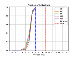
(a) GoogLeNet, Conv 1

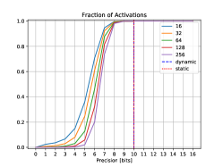
(b) GoogLeNet, 5a-1x1

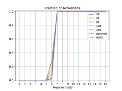
(c) SkimCaffe ResNet50, res3a_branch1

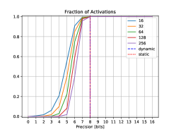
(d) SkimCaffe ResNet50, res5a_branch1

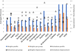
(e) Other Networks

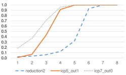
(f) Quantized 8b GoogleNet

Figure 1: Precision profiles for some conv. layers. (a)-(d) Average over multiple images. Multiple group sizes shown. "Dynamic" results for one sample image. (e) Average precisions and potential improvements for several networks. (f) Dynamic precision variability for three layers of an 8b quantized version of GoogleNet.

This section demonstrates that using per layer precisions for the activations is overly pessimistic. We demonstrate benefits for weighs and activations in Section 6.

Figures 1a-1d show precision measurements for four convolutional layers – two from each of GoogleNet and SkimCaffe-ResNet50 [23] a weight pruned network. Similar trends were observed in other networks and layers. The measurements are over 5,000 randomly selected images from the IMAGENET dataset [24]. The graphs show the cumulative distribution of the precisions needed per group of activations for various group sizes ranging from 16 to 256, where each group uses the precision needed for its least favorable activation. Two vertical lines report the precisions when considering all activation values: 1) the profile-derived (“static”) over all sample images, and 2) the one that can be detected dynamically (“dynamic”) for one randomly selected sample image to illustrate that precisions also vary per input.

Figure 1a reports measurements for conv1, the first layer of GoogleNet. The profile-determined precision is 10 bits while for one specific image all values within the layer could be represented with just 7 bits, an improvement of 30% in precision length. The cumulative distribution of the precisions needed per group of 256 activations shows that further reduction in precision is possible. For example, about 80% of these groups require 6 bits only, and about 15% just 5 bits. Smaller group sizes further reduce the effective precision, however, the differences are modest. These results suggest that picking a precision for the whole layer exacerbates the importance of a few high-magnitude activations.

The first layer usually exhibits different value behavior than the rest since it processes the direct input image to discover visual features whereas the inner layers tend to try to find correlations among features. Layer 5a-1x1 in Figure 1b shows more pronounced improvements in effective precision with the smaller group sizes. Figures 1c and 1d show that the behavior persists even in the sparse network. We include this measurement to demonstrate that dynamic precision variability is a phenomenon that is orthogonal to weight sparsity and thus of potential value to designs that target sparse neural networks.

Figure 1e compares (left Y-axis) the average effective precision with per layer profiling or with per value detection for weights and activations for additional models. These measurements are for 1000 randomly selected images from IMAGENET [24] for the image classification models [25, 26, 23, 27, 17, 28] and for 100 images from CamVid [29] for SegNet [30](segmentation), 100 and 10 inputs from Pascal VOC [31] respectively for YOLO V2 [32] (detection) and FCN8 [33] (segmentation), 10 images from CBSD68 [34, 35, 36], 10 inputs for IRCNN [37] (denoising) and VDSR [38] (super-resolution), 500 inputs from WMT14 for Seq2Seq [39] (translation), 500 inputs from COCO [40] for LRCN [41] (captioning), and 500 inputs from Flickr8k [42] for Bi-Directional LSTM [43] (captioning). The measurements are across the whole network. It also reports the reduction in work (right Y-axis) for weights and activations when per-value precision is used. The results illustrate that selecting a single precision per layer grossly overestimates the precision needed for the common case.

Figure 1f reports the distribution of precisions needed for an 8b quantized GoogleNet. Three of the longer running layers are shown which are representative of the range of behaviors seen over all layers. For reduction and icp5_out1 more than 90% of the activations can be represented with 4 bits or less. For icp7_out0 more than 90% of the activations need 6 bits a 25% reduction over 8 bits. Section 9 shows that this behavior translates into significant memory and execution time benefits.

Generally, for all the networks studied the following were observed: 1) The activation precision needed varies, more so at the first layer, 2) for all layers the precisions needed at a finer than a layer granularity are shorter than those needed for the whole layer, and 3) only a small number of activation groups require the maximum precision needed for the layer as a whole. These results motivate incorporating dynamic precision reduction in hardware accelerators.

Table 1: Average Per Layer Activation Precisions with DPRed.

Network	Effective Precision Per Layer	Reduction
AlexNet	5.39-7.36-4.22-4.40-5.81	22.59%
NiN	6.37-7.13-7.79-6.97-5.77-5.15-4.73-6.78
	-8.36-7.51-7.64-7.58	23.56%
GoogleNet	6.19-5.94-5.74-6.77-6.91-6.77-6.86-6.77
	-6.92-6.31-5.96-6.31-6.00-6.31-6.55-5.33
	-5.33-5.33-5.33-5.33-5.48-6.74-6.33-6.74
	-6.51-6.74-7.07-6.35-6.17-6.35-5.88-6.35
	-6.56-5.07-4.69-5.07-4.82-5.07-5.31-5.53
	-4.89-5.53-5.70-5.53-5.86-7.88-7.62-7.88
	-8.07-7.88-8.31-4.97-3.85-4.97-3.61-4.97-5.36	36.30%
VGG_S	5.28-5.05-5.82-3.38-4.80	38.85%
VGG_M	5.28-5.05-5.04-5.37-4.00	30.47%
VGG_19	9.05-7.69-10.04-9.00-11.08-8.74-9.65-8.29-11.55
	-10.37-12.22-11.67-11.53-11.54-10.40-5.9	21.20%

Table 2: Average Per Layer Weight Precisions with DPRed.

Network	Effective Precision Per Layer	Reduction
AlexNet	8.36-7.62-7.62-7.44-7.55	22.55%
NiN	8.85-10.29-10.21-7.65-9.13-9.04-7.63-8.65
	-8.62-7.79-7.96-8.18	19.20%
GoogleNet	9.80-10.91-9.35-10.21-10.02-9.02-10.06
	-9.34-10.29-9.61-9.73-8.63-9.93-8.65-9.64
	-9.31-9.48-8.79-9.27-8.94-9.30-9.10-9.03
	-8.25-7.27-8.56-9.15-9.26-9.17-8.21-7.32
	-8.55-9.01-9.15-9.33-8.22-9.21-8.44-9.12
	-8.54-8.68-7.47-9.11-7.93-8.86-8.52-8.59
	-7.77-8.85-8.14-8.88-8.28-8.81-7.61-8.81
	-7.52-8.40	17.27%
VGG_S	9.94-6.96-8.53-8.13-8.10	22.26%
VGG_M	9.87-7.55-8.52-8.16-8.14	21.76%
VGG_19	10.98-9.81-9.31-9.09-8.58-8.04-7.89-7.86
	-7.51-7.20-7.36-7.47-7.61-7.66-7.66-7.63	29.65%

3 Reducing Effective Precision

Tables 1 and 2 report the average precision DPRed achieves per layer which demonstrates that it can effectively reduce precisions. Due to space limitations we report results for a group size of 16 values along the channel dimension only. The effective precisions are fractional as they are averaged over all groups within the layer and weighted accordingly to their use at runtime.

4 Reducing Off-Chip Storage and Communication

The bulk of energy in DNNs is expended by off- and on-chip memory accesses. Further, when on-chip storage is limited, off-chip bandwidth can easily be the bottleneck and more easily so for the fully-connected layers due to limited data reuse. Fortunately, the variable precision needs of activations and weights can be used to reduce the amount of storage and bandwidth needed on- and off-chip. Here we limit attention to the off-chip compression scheme.

Off-chip Memory Data Container: We encode weights and activations in groups of $N$ values. We find that $N=16$ offers a good balance between compression rate and metadata overhead. Figure 2b shows the in memory data container. For each group, we determine either statically (for weights) or dynamically (using the hardware unit of Figure 2c) at the output of the previous layer or at the input source for the first layer (for the activations) the precision in bits $p_{i}$ the group needs and store that as a prefix using 4 bits, followed by the 16 values each stored using $p_{i}$ bits. In addition, to avoid storing zero values altogether, we use a 16b vector with one bit per original value to identify and store only the non-zero values off-chip. In total, this scheme requires $4+16$ bits of metadata per group of 16 values. Uncompressed these 16 values occupy 256b so the metadata overhead is far less than the benefits obtained from compressing the values for typical cases. To simplify the hardware needed, the per-group memory container can be expanded so that in total it occupies a size that is a multiple of the memory interface (64b in our experiments).

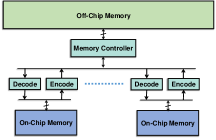
(a)

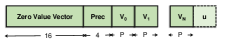
(b)

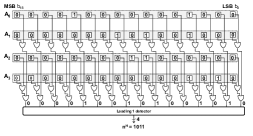
(c)

Figure 2: Using per group precisions to reduce off-chip memory bandwidth and storage.

Detecting the Per Group Precisions for Activations: Figure 2c shows how the hardware adjusts the precision at runtime for an example group of four 16b activations $A_{0}$ through $A_{3}$. It trims the unnecessary prefix bits by detecting the most significant bit position needed to represent all values within the group. The example activations can all be represented using just 12 bits as the highest bit position $n_{H}$ a 1 appears is position 11. The hardware calculates 16 signals, one per bit position, each being the OR of the corresponding bit values across all four activations. The implementation uses OR trees to generate these signals. A “leading 1” detector identifies the most significant bit that has a 1, and reports its position in 4 bits. The same method can detect $n_{L}$ – the trailing bit position needed to eliminate zero suffix bits. In practice, adjusting $n_{L}$ dynamically resulted in an negligible reduction in effective precision of less than 0.4%; profiling effectively filters the less significant noisy bits which affect all activations regardless of magnitude [9]. Accordingly, we use the profile-derived $n_{L}$ per layer. Since our networks used the ReLU all activation values are positive. The detector can be extended to handle negative values by converting them first to a sign-magnitude representation, and placing the sign at the rightmost (least significant) place. This is useful for weights and for networks that use activation functions that attenuate but not remove negative values [44, 45].

Memory Layout and Access Strategy: To minimize off-chip energy, we can size the on-chip memory buffers so that each weight and activation is accessed from off-chip once per layer [46]. In this case, the off-chip access stream is linear and contiguous and the different size of each container is no challenge. When the on-chip memory is not sufficiently large, we have to access some activations multiple times. The random access points can be easily identified at runtime when accessing them for the first time. Generally, for any given dataflow it will be possible to identify loop points either statically for the weights or dynamically for the activations and pre-record those in a small separate table.

Decompression/Compression: We use several decompression engines operating in parallel as per Figure 2a. As data is read from off-chip in chunks of 64b, the memory controller inspects the metadata header and distributes the data packets containing the values to the decompression engines each serving a different subset of the on-chip memory banks. The decompression engines expand the values to the format used in the on-chip memories and do so serially, one value at a time, avoiding the use of wide crossbars or shuffling networks. At the output of each layer, the output activations are assembled in groups in each bank and are encoded accordingly using the precision detected by the hardware of Figure 2c. The memory controller writes the resulting data containers as they become available.

Reducing On-Chip Communication: The precision reduction unit of Figure 2c can reduce communication when moving values on-chip as long as we use a bit-serial communication channel per value: values are trimmed just before the communication channel. A wide communication channel can be used to send multiple values concurrently.

Reducing On-Chip Storage: We can encode values in on-chip memory using the virtual column method of Judd et al., [47]. Values within the same precision group are spread over multiple virtual columns, one value per column. A separate virtual column is needed to specify the precision for each group. Evaluating this option is left for future work.

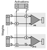
(a)

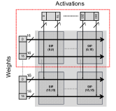
(b)

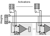
(c)

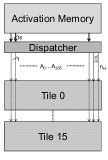
(d)

Figure 3: (a) Baseline bit-parallel accelerator. (b)-(d): DStripes: Converting Stripes to dynamically reduce activation precisions.

5 Reducing Execution Time

The fine-grain precision requirement variability of the activations and weights can be used to also boost performance and energy efficiency. Specifically, this section presents DPred Stripes or DStripes, an accelerator whose performance in convolutional layers scales proportionally with the inverse of the precision used for activations. DStripes is unique in that it adjusts the precision on-the-fly to meet the needs of only those activations that are currently being processed. Fortunately, DStripes can be implemented as a modest extension over the previously proposed Stripes [13]. Simplicity and low cost are major advantages for any new hardware proposal. We first review Stripes and an equivalent fixed-precision accelerator, and then explain the changes needed to enable dynamic precision reduction.

5.1 STRIPES and Bit-Parallel Accelerator

For clarity this discussion assumes the previously described configuration of a Stripes chip with 16 tiles, each processing 16 filters and 16 weights per filter and where the maximum precision is 16b. Figure 3a shows the tile of an equivalent fixed-precision bit-parallel accelerator BASE which is inspired by DaDianNao [1]. For clarity in this discussion we assume that all data per layer fits on-chip (Google’s TPU also uses large on-chip memories [21]). Section 6 considers the effects of reduced on-chip storage and of realistic off-chip memory systems. A Dispatcher fetches the activations from a central 4MB Activation Memory (AM) whereas a 2MB per tile slice of a Weight Memory (WM) provides the 4K weight bits that are needed per tile. In BASE, the dispatcher broadcasts 16 activations, or 256 bits per cycle. Each cycle, each BASE tile multiplies these 16 activations with 16 groups, each of 16 weights, and accumulates the results into 16 output activations. Each group of weights corresponds to a different filter and there is one weight per input activation in each group. Each BASE tile contains 16 inner-product units ($IP_{0...15}$). Each IP has several output accumulators. Data Reuse: BASE exploits data reuse both spatially and temporarily. Specifically each activation is reused across all filters, $16\times$ per tile. In addition, the output accumulators can be used used to reuse weights and activations over time by multiplexing the calculation of several output activations per tile.

In Stripes, each cycle the dispatcher broadcasts 16 sets of 16 activations to all tiles bit-serially for a total of 256 bits per cycle. Each activation set corresponds to a different input window so that the same 16 weights can be reused across groups to yield 16 output activations. As Figure 3b shows, each tile contains a grid of $16\times 16$ Serial Inner-Product units (SIPs). Each SIP performs 16 $1b\times 16b$ multiplications followed by a reduction. The SIPs along the same column share the same group of 16 single-bit activations, while the SIPs along the same row share the same 16 16b weights, as each SIP produces an output activation corresponding to a different window. Figure 3c shows one such row of SIPs. Overall, each tile accepts 256 input activations and $256\times 16=4K$ weight bits per cycle, maintaining the same number of external wire connections as BASE. Before processing a layer Stripes expects software to specify the required precision, that is the positions of the most significant and of the least significant bits (MSB and LSB respectively), $n_{H}$ and $n_{L}$. Stripes uses this precision for all activations within the layer. Since Stripes processes 256 activations bit-serially over $P_{a}$ cycles, it can ideally improve performance by $16/P_{a}$ over BASE. Data Reuse: Stripes further boosts data reuse in space and time: 1) each weight is reused across the 16 SIPs per row, and 2) weights are reused over the multiple cycles it takes to calculate their product with the corresponding activation bit-serially.

5.2 DPRed Stripes Architecture

The modest changes needed over Stripes to implement dynamic precision reduction are: 1) introducing a mechanism for detecting the precision needed per activation group, 2) adding a method of communicating the precision to the tiles, and 3) modifying the SIPs to appropriately handle starting the calculation per group at any $n_{H}$ bit position.

Precision Detection: Figure 3d shows the DStripes organization. A dispatcher reads a group of 256 activations from AM, however before communicating their values bit-serially, it first inspects them detecting the precision needed. It then communicates this precision as a 4-bit offset and as a single end of group signal. The precision is detected using the precision detection unit of Figure 2c.

To process an activation group, the dispatcher sends $n_{H}$ as the starting offset. The tiles decrement this offset every cycle. The dispatcher signals, using an end of group wire, the last cycle of processing for this group when the current offset becomes equal to $n_{L}$.

Granularity: The DStripes configurations we study detect precision for all 256 concurrently processed activations. Other arrangements are possible. For example, precision can be detected per group of 16 activations corresponding to SIPs along the same column.

Modified Serial Inner-Product Unit: The only modification needed to the SIP is the introduction of a shifter at the output of the adder tree. This shifter adjusts the adder tree output so that it can be accumulated with the running sum aligning it at the appropriate bit position. This is necessary since starting position varies per activation group.

5.3 Fully-Connected Layers

While Stripes and DStripes exploit precision variability for convolutional layers they do not do so for fully-connected layers. As a result, performance for fully-connected layers with Stripes and DStripes remains practically the same as that of BASE, but energy-efficiency suffers. This section motivates further extending Stripes and DStripes to exploit precision variability to boost performance and energy efficiency for fully-connected layers. We motivate this change by showing that: 1) indeed energy efficiency suffers in fully-connected layers (Section 5.3), and 2) precisions vary for weights in fully-connected layers (Section 5.3). The aforementioned results motivate the Tartan (TRT) extension that improves performance and energy efficiency for fully-connected layers and which complements Stripes and DStripes. For clarity this section presents TRT as an extension over Stripes.

While Stripes’s performance in fully-connected layers is virtually identical to BASE, its energy efficiency is on average $0.73\times$ with very little variation across networks. While in image classification workloads fully-connected layers represent less than 10% of the overall execution time, in other applications this is not the case. Accordingly, it is desirable to improve energy efficiency for these layers as well.

The per layer precision profiles presented here were found via the methodology of Judd et al. [9]. For the image classification convolutional neural networks, Caffe [25] was used to measure how reducing the precision of each fully-connected layer affects the network’s overall top-1 prediction accuracy over 5000 images. The networks are taken from the Caffe Model Zoo [48] and are used as-is without retraining. For fully-connected layers precision exploration was limited to cases where both $P_{w}$ and $P_{a}$ are equal (the weight and activation precision ranges differ). For convolutional layers only the activation precision is adjusted since none of the designs we consider can further boost performance when reducing the weight precisions. While reducing the weight precision for convolutional layers can reduce their memory footprint [47], we do not explore this option in this evaluation. For NeuralTalk, we measure BLEU scores when compared with the ground truth. For Denoise, we measure PSNR, and define >99% accuracy as a drop of no more than 0.04dB.

Table 3 reports the resulting per layer precisions. The ideal speedup columns report the performance improvement that would be possible if execution time could be reduced proportionally with precision compared to a 16-bit bit-parallel baseline. For the fully-connected layers, the precisions required range from 8 to 10 bits and the potential for performance improvement is $1.64\times$ on average. Given that the precision variability for fully-connected layers is relatively low (ranges from 8 to 11 bits) one may be tempted to conclude that an 11-bit BASE variant may be an appropriate compromise. However, given that the precision variability is much larger for the convolutional layers (range is 5 to 13 bits) the performance with a fixed precision datapath would be far below the ideal. Section 6 shows that the incremental cost of TRT over Stripes is well justified given the benefits.

Table 3: Per layer precision profiles needed to maintain the same accuracy as in the baseline. Ideal: Potential speedup with bit-serial processing of activations over a 16-bit bit-parallel baseline without dynamic adaptation.

Convolutional Layers
Network	Activation Precision in Bits	Ideal
	100% Accuracy	Speedup
AlexNet	9-8-5-5-7	2.38
VGG_S	7-8-9-7-9	2.04
VGG_M	7-7-7-8-7	2.23
VGG_19	12-12-12-11-12-10-11-11-13-12-13-13-13-13-13-13	1.35
NeuralTalk	-	-
Denoise	-	-
Fully Connected Layers
	Act. & Weight Precision in Bits	Ideal
100% Accuracy		Speedup
AlexNet	10-9-9	1.66
VGG_S	10-9-9	1.64
VGG_M	10-9-9	1.64
VGG_19	10-9-9	1.63
NeuralTalk	11 (all iterations)	1.45
Denoise	12 (all layers)	1.33

5.3.1 TARTAN

Unfortunately, since there is no weight reuse in fully-connected DStripes cannot reuse the same weight over multiple windows. In DStripes performance in fuly-connected layers is limited by the number of cycles needed to load a different set of weights per SIP column [13]. TRT overcomes this limitation and boosts performance even for fully-connected layers by exploiting weight and activation precisions. We use Figure 4a to explain the concept behind TRT’s operation. The figure shows a row of SIPs (similar to Figure 3c) and focuses on the first weight input only. Whereas in Stripes the 16b weight input to the AND gates was coming directly from the WM connection here it is connected to a 16b Weight Register (WR). A multiplexer selects from where the WR can load its contents. The first option is to do so directly from the WM wires as in Stripes. This maintains the functionality needed for convolutions. An extra pipeline stage is needed to accommodate loading first to WR (stage 1) and then “multiplying” with the activation (stage 2). The second option is to load WR from the 16b Serial Weight Register (SWR). The SWR has a single input wire connection to the Weight Memory which is different per SIP. The first SIP in the row connects to wire 0 while the last to wire 15. SWR is a serial-load register and it can load a new weight value of $p$ bits bit-serially over $p$ cycles. Given that each SWR connects to a different Weight Memory wire, they can all concurrently load a different $p$ bit weight value over the same $p$ cycles. Each SIP can then copy its SWR held weight into its WR and proceed with processing the corresponding activations bit serially. Concurrently with processing the activations, the SWR can proceed to load the next set of weights. Accordingly, loading weights into the SWRs and processing the ones in the WRs form a two “stage” pipeline. The first “stage” of this pipeline requires $P_{w}$ cycles to load a new set of weights since the weights are loaded bit-serially. The second “stage” of the pipeline requires $P_{a}$ to process the current set of weights and activations since it multiplies activations bit-serially. As a result, it is the maximum precision of the weights or the activations that will dictate the number of cycles needed to process each group of activations.

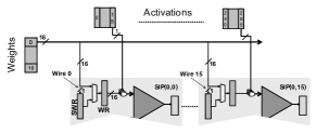
(a)

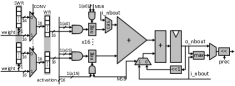
(b)

Figure 4: TRT Tile and SIP.

Since there are 16 weights per SIP, the SWR and WR are implemented each as a vector of 16 16-bit subregisters. The remainder of this section explains how TRT processes convolutional and fully-connected layers. For clarity, in what follows the term brick refers to a set of 16 elements of a 3D activation or weight array input which are contiguous along the channel dimension, e.g., $a(x,y,i)...a(x,y,i+15)$. Bricks will be denoted by their origin element with a $B$ subscript, e.g., $a_{B}(x,y,i)$. The size of a brick is a design parameter.

Convolutional Layers: Processing is identical to Stripes and starts by reading in parallel 256 weights from the Weight Memory as in Stripes, and loading the 16 per SIP row weights in parallel to all SWRs in the row.

Fully-Connected Layers: Processing starts by loading bit-serially and in parallel over $P_{w}$ cycles 4K weights into the 256 SWRs, 16 per SIP. Each SWR per row gets a different set of 16 weights as each subregister is connected to one out of the 256 wires of the Weight Memory output bus for the SIP row (as in BASE there are $256\times 16=4K$ wires). Once the weights have been loaded, each SIP copies its SWR to its SW and multiplication with the input activations can then proceed bit-serially over $P_{a}^{L}$ cycles. Assuming that there are enough output activations so that a different output activation can be assigned to each SIP, the same input activation brick can be broadcast to all SIP columns. That is, each TRT tile processes one activation brick $a_{B}(i)$ bit-serially to produce 16 output activation bricks $o_{B}(i)$ through $o_{B}(i\times 16)$, one per SIP column. Loading the next set of weights can be done in parallel with processing the current set, thus execution time is constrained by $P_{max}=max(P_{a},P_{w})$. Thus, a TRT tile produces 256 partial output activations every $P_{max}$ cycles, a speedup of $16/P_{max}$ over BASE since a BASE tile always needs 16 cycles to do the same.

Cascade Mode: TRT is underutilized in fully-connected layer with less than 4K output activations. Some networks have layers with as little as 2K outputs. To avoid underutilization, the SIPs along each row are cascaded into a daisy-chain, where the output of one can feed into an input of the next via a multiplexer. This way, the computation of an output can be sliced over the SIPs along the same row: Each SIP processes only a portion of the input activations resulting into several partial output activations along the SIPs on the same row. Over the next $np$ cycles, where $np$ the number of slices used, the $np$ partial outputs are added. The user can chose any number of slices up to 16, so that TRT can be fully utilized even when there are just 256 outputs.

Other Layers: TRT like Stripes can process the additional layers needed by the studied networks. The tile includes hardware support for max pooling similar to Stripes. An activation function unit is present at the output in order to apply nonlinear activations before writing back to AM.

SIP and Other Components: Figure 4b shows TRT’s SIP which multiplies 16 activation bits, one bit per activation, by 16 weights to produce an output activation. Two registers, a Serial Weight Register (SWR) and a Weight Register (WR), each contain 16 16-bit sub-registers. Each SWR sub-register is a shift register with a single bit connection to one of the weight bus wires that is used to read weights bit-serially for FCLs. Each WR sub-register can be parallel loaded from either the weight bus or the corresponding SWR sub-register to process convolutional or fully-connected layers respectively. The SIP includes 256 2-input AND gates that multiply the weights in the WR with the incoming activation bits, and a $16\times 16b$ adder tree that sums the partial products. A final adder plus a shifter accumulate the adder tree results into the output register. A multiplexer at the first input of the adder tree implements the cascade mode supporting slicing the output activation computation along the SIPs of a single row. Each SIP also includes a comparator (max) to support max pooling layers. A shifter between the output of the adder tree and the input to the accumulator can be added to support DPRed.

As in Stripes there is a central AM and 16 tiles. A Dispatcher unit is tasked with reading input activations from AM always performing eDRAM-friendly wide accesses. It transposes each activation and communicates each a bit a time over the global interconnect. For convolutional layers the dispatcher has to maintain a pool of multiple activation bricks, each from different window, which may require fetching multiple rows from AM. However, since a new set of windows is only needed every $P_{a}$ cycles, the dispatcher can keep up for the layers studied. For fully-connected layers one activation brick is sufficient. A Reducer per title is tasked with collecting the output activations and writing them to AM. Since output activations take multiple cycles to produce, there is sufficient bandwidth to sustain all 16 tiles.

Coarser Bit Granularity Processing: To improve TRT’s area and power efficiency, the number of activation bits processed at once can be adjusted at design time. Such designs need fewer SIPs and shorter wires. However, they forgo some of the performance potential as they force the activation precisions to be a multiple of the number of bits that they process per cycle.

5.4 DPRed Loom

Dynamic precision variability can also benefit Loom [22], an architecture that exploits precision variability both in activations and weights which is faster and more energy efficient than Stripes for smaller configurations. The original design, which uses per-layer precisions, can be extended utilizing the mechanism described in Section 5.2 to take advantage of per group precisions for both weights and activations.

6 Evaluation

We first assume that all data fits on chip using the memory configuration of DaDianNao [2]. Having identified a reasonable compute configuration we then study restricted on-chip memory hierarchies and the effect of off-chip memory demonstrating that DPRed greatly helps with alleviating stalls due to off-chip accesses.

All accelerators were modeled using the same methodology for consistency. A custom cycle-accurate simulator models execution time. Computation was scheduled as described in Stripes to maximize energy efficiency for BASE [13]. To estimate power and area, all designs were synthesized with the Synopsys Design Compiler [49] for a TSMC 65nm library and laid out with Cadence Encounter. Circuit activity was captured with ModelSim and fed into Encounter for power estimation. All designs operate at 980 MHz. The SRAM activation buffers were modeled using CACTI [50]. The AM and WM eDRAM area and energy were modeled with Destiny [51]. Three design corner libraries were considered prior to layout. The typical case library was chosen for layout since bit-serial designs are affected less by the worst-case design corner. Accordingly, the relative benefits with DPRed over BASE are underestimated. DStripes and TRT improve energy efficiency and performance for all design corners.

Given that DStripes improves performance only for conv. layers, and that TRT performs identically to DStripes for conv layers while improving performance only for fully-connected layers, a different set of DNNs is used during the evaluation of the two techniques. For DStripes measurements were performed over a set of ImageNet Classification CNNs: AlexNet, GoogleNet, Nin, VGG_S, VGG_M, and VGG_19. For these networks conv. layers account for more than 90% of the execution time. For TRT the evaluation omits NiN and GoogleNet since the former has no fully-connected layers and their usage in the latter is not significant. Instead NeuralTalk [52] and Denoise [53] are included that are dominated by fully-connected layers. NeuralTalk uses long short-term memory to automatically generate image captions. Denoise is a 5-layer Multilayer Perceptron that implements image denoising aiming to reproduce the results of the state-of-the-art BM3D denoising algorithm [54].

6.1 DStripes

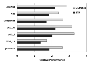
(a)

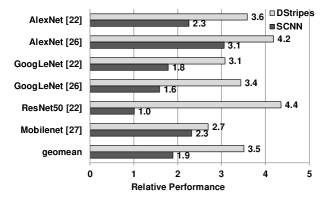
(b)

Figure 5: DStripes: Speedup over BASE in Convolutional Layers

Performance: Figure 5a shows the resulting speedup with DStripes alone and over the equivalently configured BASE and Stripes. Since DStripes improves performance only for conv. layers these measurements are restricted to conv. layers only. On average, dynamic precision reduction boosts performance over Stripes by 41% since DStripes proves $2.61\times$ faster than BASE.

Energy Efficiency: As Table 4 shows DStripes greatly improves energy efficiency over BASE and Stripes. The dispatcher has to communicate less bits and the units have to perform fewer calculations. On average, compared to BASE, Stripes and DStripes are $1.84\times$ and $1.38\times$ more energy efficient respectively.

Area: In the interest of space, we omit the detailed area results here and present those for the combination of DStripes and TRT instead in the respective section. The overall area overhead of dynamic precision reduction is less than 1% over Stripes and as a result DStripes is $1.32\times$ larger than BASE. Given that DStripes is $2.61\times$ faster, the performance over area ratio is superlinear with DStripes. Utilizing 32% more area in BASE would at best increase performance proportionally. However, in practice the speedup will be a lot less due to filter and input dimensions and filter count.

Table 4: Convolutional Layers: Energy Efficiency of DStripes vs. BASE and vs. Stripes (higher is better)

Network	vs. BASE	vs. Stripes
AlexNet	1.98	1.26
NiN	1.68	1.27
GoogleNet	1.86	1.53
VGG_M	2.22	1.40
VGG_S	2.31	1.58
VGG_19	1.20	1.24
GEOMEAN	1.84	1.38

Table 5: Execution time and energy efficiency improvement with DStripes_T compared to BASE.

	Fully Connected Layers		Convolutional Layers
	Perf	Eff	Perf	Eff
AlexNet	1.61	1.10	2.81	1.28
VGG_S	1.61	1.09	3.26	1.49
VGG_M	1.61	1.10	3.15	1.44
VGG_19	1.60	1.09	1.70	0.77
NeuralTalk	1.42	1.01	-	-
Denoise	1.30	0.92	-	-
geomean	1.52	1.05	2.65	1.21

6.2 Pruned Models

Pruning is sometimes possible and it converts several weights into zeros. Past work has exploited pruning to reduce work. Figure 5b compares the performance of DStripes and SCNN [5] for a set of pruned models [23, 27]. For both designs we assume infinite off-chip bandwidth giving an advantage to SCNN since DPRed reduces traffic more than zero compression. SCNN removes all products where the activation or the weight is zero. The reasons why DStripes outperforms SCNN are: 1) SCNN’s performance is limited by inter- and intra-tile fragmentation [5], while 2) DStripes targets all activations where the potential for work reduction is higher than the work reduction potential from targeting those values that are zero. However, Dynamic Precision Reduction is compatible with SCNN and we have experimented with replacing the bit-parallel multiply-accumulate units in SCNN with bit-serial ones while increasing the number of tiles. Unfortunately, the benefits are limited since the higher tile count exacerbates inter-tile load imbalance. Addressing this imbalance is left for future work.

6.3 DStripes and TARTAN

Performance: We evaluate the combination of DStripes and TRT denoted as DStripes_T. Table 5 reports DStripes_T’s performance and energy efficiency relative to BASE for the precision profiles in Table 3 separately for fully-connected layers, convolutional layers, and the whole network. Denoise has no convolutional layers. NeuralTalk uses a modified convolutional neural network (based on VGG_16 in this implementation) to recognize objects before the LSTM stage; we do not evaluate that phase as it is similar to the other image classifiers.

On fully-connected layers DStripes_T yields, on average, a speedup of $1.52\times$. For conv. layers DStripes_T improves performance by $2.65\times$. There are two main reasons DStripes_T does not reach the ideal speedup: dispatch overhead and under-utilization. During the initial $P_{w}$ cycles the serial weight loading process prevents any useful products to be performed. This represents less than 2% for any given network, although it can be as high as 6% for the smallest layers. Underutilization can happen when the number of outputs is not a power of two or lower than 256.

Energy Efficiency As Table 5 reports, the average efficiency improvement with DStripes_T across all networks and layers is $1.19\times$. DStripes_T is more efficient than BASE for all layers. Overall, efficiency primarily comes from the reduction in effective computation due to reduced precisions. Furthermore, the amount of data that has to be transmitted from the WM and the traffic between the AM and the SIPs is decreased proportionally with the chosen precision.

Area: Table 6 reports the area breakdown of DStripes_T and BASE. Over the full chip, DStripes_T needs $1.51\times$ the area compared to BASE while delivering on average a $2.59\times$ speedup. Generally, performance would scale sublinearly with area for BASE due to underutilization.

Sensitivity to Precision Resolution: Table 7 reports performance for the DStripes_T variant of Section 4 that processes 2 bits per cycle in as half as many total SIPs. The previously quoted precisions are rounded up to the next multiple of two. This design always improves performance compared to BASE. Compared to the 1-bit DStripes_T performance is slightly lower, however this can be a good trade-off given the reduced cost and improved energy efficiency. Overall, there are two forces at work: There is performance potential lost due to rounding all precisions to an even number, and there is performance benefit by requiring less parallelism. The time needed to serially load the first bundle of weights is also reduced. The layout of DStripes_T’s 2-bit variant requires only 26.0% more area than BASE (Table 6) while improving energy efficiency in fully-connected layers by $1.24\times$ on average ($1.44\times$ across all layer types).

Table 6: Area Breakdown for DStripes_T and BASE

	DStripesT	DStripesT 2-bit	BASE
Inner-Product Units	58.60 (48.21%)	38.32 (37.84%)	17.85 (22.20%)
Weight Memory	48.11 (39.58%)	48.11 (47.50%)	48.11 (59.83%)
Act. Input Buffer	3.66 (3.01%)	3.66 (3.61%)	3.66 (4.55%)
Act. Output Buffer	3.66 (3.01%)	3.66 (3.61%)	3.66 (4.55%)
Activation Memory	7.13 (5.87%)	7.13 (7.04%)	7.13 (8.87%)
Dispatcher	0.39 (0.32%)	0.39 (0.39%)	-
Total	121.55 (100%)	101.28 (100%)	80.41 (100%)
Normalized Total	$1.51\times$	$1.26\times$	$1.00\times$

Table 7: Relative performance of the 2-bit DStripes_T

	Fully Connected Layers		Convolutional Layers
	vs. BASE	vs. 1b DStripesT	vs. BASE	vs. 1b DStripesT
AlexNet	+58%	-2.06%	+164%	-7.11%
VGG_S	+59%	-1.25%	+191%	-13.27%
VGG_M	+63%	+1.12%	+181%	-12.57%
VGG_19	+59%	-0.97%	+63%	-4.93%
NeuralTalk	+30%	-9.09%	-	-
Denoise	+29%	-1.10%	-	-
geomean	+49%	-2.28%	+144%	-9.53%

Figure 6: Offchip traffic reduction with compression schemes. Overhead for the compression metadata is reported as a percentage of the compressed traffic. The four rightmost models use per-layer precision aware 8-bit quantization.

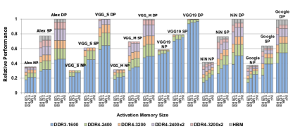
Figure 7: Performance of DStripes with different memory technologies, off-chip compression schemes, and activation memory sizes for convolutional layers.

Table 8: DStripes: Speedup over an 8-bit baseline in all layers with 8-bit quantization

Precision Oblivious Quant.		Precision Aware Quant.
Iso - Peak Compute Bandwidth		Iso-Area
Name	Rel. Perf.	Name	Rel. Perf.
AlexNet	1.11	AlexNet [26]	1.62
NiN	1.36	GoogleNet [26]	1.54
GoogleNet	1.28	BiLSTM	1.76
VGG_M	1.15	SegNet	2.50
VGG_S	1.22	geomean	1.82
VGG_19	1.44
ResNet50	1.39
Mobilenet	1.27
geomean	1.27

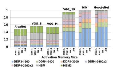
Figure 8: Performance of DStripes with different memory technologies and activation memory size for convolutional layers and fully connected layers.

6.4 Memory Hierarchy

We consider the effects of off-chip bandwidth and the effectiveness of DPRed for off-chip bandwidth amplification. We use 320KB of WM per tile which is sufficient so that DStripes can read each weight only once from off-chip and per layer [46]. Figures 7 show the effect on the performance of DStripes for different on-chip AM sizes, compression schemes ($x$-axis), and off-chip memory technologies (stacked bars). We consider three compression schemes: 1) No Compression (NP), 2) precision-based using profile-derived per layer precisions (SP) [47], and 3) our per group precision-based (DP). Performance is normalized to the configuration where all activations fit on chip (INF) — the configurations used thus far. Figure 7 reports relative performance for the convolutional layers only, while Figure 8 reports relative performance for all layers.

Overall, the choice of external memory impacts performance significantly more than the choice of the on-chip AM. The results show that our compression scheme greatly boosts performance by reducing the impact of off-chip traffic. For the convolutional layers DStripes when used with our compression manages to maintain most its performance benefits even with 2 channels of DDR4-3200 memory. With HBM, which would be appropriate given the peak compute capability of this configuration, the performance is within 2% of the ideal. Off-chip memory is the bottleneck for fully-connected layers. However, using HBM or HBM2 preserves most of the overall benefits provided that our compression scheme is used. Finally, Figure 6 reports the relative off-chip traffic normalized to no compression (Base). Our compression scheme reduces traffic to 55% for GoogleNet, 60% for BiLSTM and to less than 40% for the remaining networks.

6.5 DPRed Loom

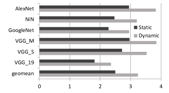
Figure 9: LOOM: Comparison between static and dynamic precisions (with LPDDR4-4267)

Figure 9 compares the performance of Loom when using dynamic vs. static per-layer precisions with a LPDDR4-4267 off-chip memory. We use the AM and WM memories suggested by Sharify et al. [22], processing 2048 weights and 256 activations concurrently bit-serially.

6.6 8-bit Quantization

Table 9: Area and power consumption of DStripes_T normalized to BASE for 8-bit configuration

	DStripesT (8-bit)	BASE (8-bit)
Normalized Total Area	$1.05\times$	$1.00\times$
Normalized Total Compute Area	$1.87\times$	$1.00\times$
Normalized Power	$1.64\times$	$1.00\times$

Table 8 reports performance for 8b quantized models. We report results for two quantization approaches. The first two columns report results with the 8-bit quantized representation used in Tensorflow [11, 55]. This quantization uses 8 bits to specify arbitrary minimum and maximum limits per layer for the activations and the weights separately, and maps the 256 available 8-bit values linearly into the resulting interval. The second set of columns use precision aware quantization where quantization does not unnecessarily expand a range that can fit in less than 8b to the full 8b range. We perform an iso-area comparison only for the last set of models. That is, we scale the baseline’s compute resources to use at least as much area as that of DStripes; instead of 1.87x as per Table 9 we scale the area of the baseline compute units to 2x. We do not scale the memories since this does not provide a benefit in this evaluation, as all data fits on chip. In the time alloted we were able to quantize the four models shown which include a captioning LSTM and a segmentation CNN.

Table 9 reports the relative area and instantaneous power of the baseline and DStripes when scaled to 8b. Scaling to 8b reduces area and power overheads for DStripes considerably since less pipelining is needed to achieve the frequency target, and quadratic scaling characteristics are diminished.

Table 10: LOOM: Speedup over an 8-bit baseline in all layers for 8-bit networks

Name	Rel. Perf.
AlexNet [26]	2.70
Goog [26]	2.13
BiLSTM	2.67
SegNet	4.07
GeoMean	2.81

Finally, Table 10 compares the performance of DPRed LOOM [22] vs. an throughput-equivalent bit-parallel baseline for the 8b precision-aware quantized models.

7 Related Work

Distributed Arithmetic (DA), which computes inner products bit-serially, has been used in the design of Digital Signal Processors [56], including designs with application-specific dynamic precision detection [57]. DA precomputes and stores in a table all combinations of coefficients. This is intractable for the weights of DNN as they are too many.

Pragmatic uses a similar organization to Stripes and thus DStripes but its performance on convolutional layers depends only on the non-zero activation bits [16]. DPRed can improve energy efficiency for Pragmatic by reducing the number of bits sent from off-chip memory and from AM to the tile. DStripes represents a different area vs. efficiency vs. performance trade-off than Pragmatic. The Efficient Inference Engine (EIE) uses weight pruning and sharing, zero activation elimination, and network retraining to drastically reduce the weight storage and communication when processing fully-connected layers [58]. This is an aggressive form of weight compression requiring a secondary table lookup to decode each weight. DPRed attacks activations also and thus a phenomenon that is mostly orthogonal to those EIE exploits. It may be possible to incorporate DStripes’s approach within the tile of EIE. For fully-connected layers, TRT offers lightweight memory compression. An appropriately configured EIE will may outperform TRT for fully-connected layers, provided that the network is pruned and retrained. However, while pruning in earlier CNNs resulted in sparsity in the 80% to 90% range, for more recent networks sparsity is lower, in the 50% to 60% range [27, 23].

Bit-Fusion takes advantage of per layer precisions using a spatial design instead of the bit-serial design of Stripes [14]. DStripes adapts precisions at a finer granularity and dynamically. Bit-Fusion can benefit from the off-chip compression offered by DPRed.

Advances at the algorithmic level would impact DStripes and TRT as well or may even render them obsolete. For example, work on using binary weights [59] would obviate the need for an accelerator whose performance scales with weight precision.

New datatypes such as Intel’s Flexpoint [60] or Tensorflow’s bfloat16 [61] have been introduced as lower precision alternatives to 32-bit floating point for use in deep neural networks. They provide a wider range than fixed-point representations and target primarily training. They are statically sized data representations and require 7, 8 or 16 bits of mantissa, and 8 bits of exponent regardless of the magnitude of the value stored. The models will still exhibit a lopsided value distribution and will natural exhibit variable precision requirements per layer. Accordingly, DPRed can be applied to both the mantissa and exponent to adjust the least significant bits used after profiling has been used to trim the precision needed per layer.

Quantization to lower precisions has been used to reduce the memory and computation cost in neural networks. For example, Google’s Tensor Processing Unit (TPU) uses quantization to represent values using 8 bits [21] to support TensorFlow [61]. Nvidia TensorRT also supports quantization to 8-bits [62]. However, quantization is not without its drawbacks. Although a fixed precision may be suitable for certain networks, using a fixed quantization scheme may not be optimal/sufficient for all problems, e.g., those using RNNs [62]or computational imaging tasks performing per-pixel prediction, e.g., [38, 37] which process raw sensor data of 12b or more, or even some image classification tasks and speech processing [63]. Therefore, flexible precision support is important to generalize across different applications.While quantization attenuates some of the expected benefits with DPRed the underlying phenomenon that DPRed exploits persists: there will be few high values. This is the reason why it benefits even 8b quantized image networks. Further, DStripes and LOOM offer benefits even for those networks that can be quantized further even for non powers of two precisions, e.g., [64] without requiring all networks to be quantized to obtain benefits. Park et al., present an outlier aware accelerator design where a set of limited high-precision execution units are used to process those neurons that require them whereas the bulk of computations happen in lower precision units [15]. For this purpose, the weights are quantized and partitioned statically. DPRed works with any network whether quantized or not and adapts the precisions of both weights and activations. For this reason it could be beneficial even for the above reference accelerator.

8 Conclusion

We believe that dynamic precision reduction opens up several directions for future work including how to combine with other accelerator engines, how it can boost the effectiveness of algorithms for pruning or for precision reduction or quantization of weights and of activations, and whether it can be exploited to accelerate training as well. The accelerators we proposed do not require any changes to the input network to deliver benefits. However, they do reward any advances in precision reduction including linear quantization and thus if deployed will provide an incentive for further innovation towards networks of extremely low precision.

References

- [1] T. Chen, Z. Du, N. Sun, J. Wang, C. Wu, Y. Chen, and O. Temam, “Diannao: A small-footprint high-throughput accelerator for ubiquitous machine-learning,” in Proceedings of the 19th international conference on Architectural support for programming languages and operating systems, 2014.
- [2] Y. Chen, T. Luo, S. Liu, S. Zhang, L. He, J. Wang, L. Li, T. Chen, Z. Xu, N. Sun, and O. Temam, “Dadiannao: A machine-learning supercomputer,” in Microarchitecture (MICRO), 2014 47th Annual IEEE/ACM International Symposium on, pp. 609–622, Dec 2014.
- [3] Chen, Yu-Hsin and Krishna, Tushar and Emer, Joel and Sze, Vivienne, “Eyeriss: An Energy-Efficient Reconfigurable Accelerator for Deep Convolutional Neural Networks,” in IEEE International Solid-State Circuits Conference, ISSCC 2016, Digest of Technical Papers, pp. 262–263, 2016.
- [4] S. Han, X. Liu, H. Mao, J. Pu, A. Pedram, M. A. Horowitz, and W. J. Dally, “EIE: Efficient Inference Engine on Compressed Deep Neural Network,” arXiv:1602.01528 [cs], Feb. 2016. arXiv: 1602.01528.
- [5] A. Parashar, M. Rhu, A. Mukkara, A. Puglielli, R. Venkatesan, B. Khailany, J. Emer, S. W. Keckler, and W. J. Dally, “Scnn: An accelerator for compressed-sparse convolutional neural networks,” in Proceedings of the 44th Annual International Symposium on Computer Architecture, ISCA ’17, (New York, NY, USA), pp. 27–40, ACM, 2017.
- [6] J. Albericio, P. Judd, T. Hetherington, T. Aamodt, N. E. Jerger, and A. Moshovos, “Cnvlutin: Ineffectual-neuron-free deep neural network computing,” in 2016 IEEE/ACM International Conference on Computer Architecture (ISCA), 2016.
- [7] S. Zhang, Z. Du, L. Zhang, H. Lan, S. Liu, L. Li, Q. Guo, T. Chen, and Y. Chen, “Cambricon-x: An accelerator for sparse neural networks,” in Proceedings of the 49th International Symposium on Microarchitecture, 2016.
- [8] J. Kim, K. Hwang, and W. Sung, “X1000 real-time phoneme recognition VLSI using feed-forward deep neural networks,” in 2014 IEEE International Conference on Acoustics, Speech and Signal Processing (ICASSP), pp. 7510–7514, May 2014.
- [9] P. Judd, J. Albericio, T. Hetherington, T. Aamodt, N. E. Jerger, R. Urtasun, and A. Moshovos, “Reduced-Precision Strategies for Bounded Memory in Deep Neural Nets, arXiv:1511.05236v4 [cs.LG] ,” arXiv.org, 2015.
- [10] M. Courbariaux, Y. Bengio, and J.-P. David, “BinaryConnect: Training Deep Neural Networks with binary weights during propagations,” ArXiv e-prints, Nov. 2015.
- [11] P. Warden, “Low-precision matrix multiplication.” https://petewarden.com, 2016.
- [12] G. Venkatesh, E. Nurvitadhi, and D. Marr, “Accelerating deep convolutional networks using low-precision and sparsity,” CoRR, vol. abs/1610.00324, 2016.
- [13] P. Judd, J. Albericio, T. Hetherington, T. Aamodt, and A. Moshovos, “Stripes: Bit-serial Deep Neural Network Computing ,” in Proceedings of the 49th Annual IEEE/ACM International Symposium on Microarchitecture, MICRO-49, 2016.
- [14] H. Sharma, J. Park, N. Suda, L. Lai, B. Chau, V. Chandra, and H. Esmaeilzadeh, “Bit fusion: Bit-level dynamically composable architecture for accelerating deep neural network,” in ISCA, pp. 764–775, IEEE Computer Society, 2018.
- [15] E. Park, D. Kim, and S. Yoo, “Energy-efficient neural network accelerator based on outlier-aware low-precision computation,” in ISCA, pp. 688–698, IEEE Computer Society, 2018.
- [16] J. Albericio, A. Delmás, P. Judd, S. Sharify, G. O’Leary, R. Genov, and A. Moshovos, “Bit-pragmatic deep neural network computing,” in Proceedings of the 50th Annual IEEE/ACM International Symposium on Microarchitecture, MICRO-50 ’17, (New York, NY, USA), pp. 382–394, ACM, 2017.
- [17] F. N. Iandola, M. W. Moskewicz, K. Ashraf, S. Han, W. J. Dally, and K. Keutzer, “Squeezenet: Alexnet-level accuracy with 50x fewer parameters and <1mb model size,” CoRR, vol. abs/1602.07360, 2016.
- [18] M. Zhu and S. Gupta, “To prune, or not to prune: exploring the efficacy of pruning for model compression,” ArXiv e-prints, Oct. 2017.
- [19] A. Delmas, P. Judd, S. Sharify, and A. Moshovos, “Dynamic stripes: Exploiting the dynamic precision requirements of activation values in neural networks,” CoRR, vol. abs/1706.00504, 2017.
- [20] B. Moons, R. Uytterhoeven, W. Dehaene, and M. Verhelst, “Envision: A 0.26-to-10tops/w subword-parallel dynamic-voltage-accuracy-frequency-scalable convolutional neural network processor in 28nm fdsoi,” in IEEE Solid-State Circuits Conference (ISSCC), 2017.
- [21] N. P. Jouppi, C. Young, N. Patil, D. Patterson, G. Agrawal, R. Bajwa, S. Bates, S. Bhatia, N. Boden, A. Borchers, R. Boyle, P.-l. Cantin, C. Chao, C. Clark, J. Coriell, M. Daley, M. Dau, J. Dean, B. Gelb, T. V. Ghaemmaghami, R. Gottipati, W. Gulland, R. Hagmann, C. R. Ho, D. Hogberg, J. Hu, R. Hundt, D. Hurt, J. Ibarz, A. Jaffey, A. Jaworski, A. Kaplan, H. Khaitan, D. Killebrew, A. Koch, N. Kumar, S. Lacy, J. Laudon, J. Law, D. Le, C. Leary, Z. Liu, K. Lucke, A. Lundin, G. MacKean, A. Maggiore, M. Mahony, K. Miller, R. Nagarajan, R. Narayanaswami, R. Ni, K. Nix, T. Norrie, M. Omernick, N. Penukonda, A. Phelps, J. Ross, M. Ross, A. Salek, E. Samadiani, C. Severn, G. Sizikov, M. Snelham, J. Souter, D. Steinberg, A. Swing, M. Tan, G. Thorson, B. Tian, H. Toma, E. Tuttle, V. Vasudevan, R. Walter, W. Wang, E. Wilcox, and D. H. Yoon, “In-datacenter performance analysis of a tensor processing unit,” in Proceedings of the 44th Annual International Symposium on Computer Architecture, ISCA ’17, (New York, NY, USA), pp. 1–12, ACM, 2017.
- [22] S. Sharify, A. D. Lascorz, K. Siu, P. Judd, and A. Moshovos, “Loom: Exploiting weight and activation precisions to accelerate convolutional neural networks,” in Proceedings of the 55th Annual Design Automation Conference, DAC ’18, (New York, NY, USA), pp. 20:1–20:6, ACM, 2018.
- [23] J. Park, S. Li, W. Wen, P. T. P. Tang, H. Li, Y. Chen, and P. Dubey, “Faster CNNs with Direct Sparse Convolutions and Guided Pruning,” in 5th International Conference on Learning Representations (ICLR), 2017.
- [24] O. Russakovsky, J. Deng, H. Su, J. Krause, S. Satheesh, S. Ma, Z. Huang, A. Karpathy, A. Khosla, M. Bernstein, A. C. Berg, and L. Fei-Fei, “ImageNet Large Scale Visual Recognition Challenge,” arXiv:1409.0575 [cs], Sept. 2014. arXiv: 1409.0575.
- [25] Y. Jia, E. Shelhamer, J. Donahue, S. Karayev, J. Long, R. Girshick, S. Guadarrama, and T. Darrell, “Caffe: Convolutional architecture for fast feature embedding,” arXiv preprint arXiv:1408.5093, 2014.
- [26] K. He, X. Zhang, S. Ren, and J. Sun, “Deep residual learning for image recognition,” CoRR, vol. abs/1512.03385, 2015.
- [27] Yang, Tien-Ju and Chen, Yu-Hsin and Sze, Vivienne, “Designing Energy-Efficient Convolutional Neural Networks using Energy-Aware Pruning,” in IEEE Conference on Computer Vision and Pattern Recognition (CVPR), 2017.
- [28] A. G. Howard, M. Zhu, B. Chen, D. Kalenichenko, W. Wang, T. Weyand, M. Andreetto, and H. Adam, “Mobilenets: Efficient convolutional neural networks for mobile vision applications,” CoRR, vol. abs/1704.04861, 2017.
- [29] G. J. Brostow, J. Fauqueur, and R. Cipolla, “Semantic object classes in video: A high-definition ground truth database,” Pattern Recognition Letters, vol. xx, no. x, pp. xx–xx, 2008.
- [30] V. Badrinarayanan, A. Kendall, and R. Cipolla, “Segnet: A deep convolutional encoder-decoder architecture for image segmentation,” IEEE Transactions on Pattern Analysis and Machine Intelligence, 2017.
- [31] M. Everingham, S. M. A. Eslami, L. Van Gool, C. K. I. Williams, J. Winn, and A. Zisserman, “The pascal visual object classes challenge: A retrospective,” International Journal of Computer Vision, vol. 111, pp. 98–136, Jan. 2015.
- [32] J. Redmon and A. Farhadi, “YOLO9000: better, faster, stronger,” CoRR, vol. abs/1612.08242, 2016.
- [33] E. Shelhamer, J. Long, and T. Darrell, “Fully convolutional networks for semantic segmentation,” IEEE Transactions on Pattern Analysis and Machine Intelligence, vol. 39, pp. 640–651, April 2017.
- [34] S. Roth and M. J. Black, “Fields of experts: a framework for learning image priors,” in 2005 IEEE Computer Society Conference on Computer Vision and Pattern Recognition (CVPR’05), vol. 2, pp. 860–867 vol. 2, June 2005.
- [35] M. Bevilacqua, A. Roumy, C. Guillemot, and M. L. Alberi-Morel, “Low-complexity single-image super-resolution based on nonnegative neighbor embedding,” 2012.
- [36] R. Zeyde, M. Elad, and M. Protter, “On single image scale-up using sparse-representations,” in Curves and Surfaces (J.-D. Boissonnat, P. Chenin, A. Cohen, C. Gout, T. Lyche, M.-L. Mazure, and L. Schumaker, eds.), (Berlin, Heidelberg), pp. 711–730, Springer Berlin Heidelberg, 2012.
- [37] K. Zhang, W. Zuo, S. Gu, and L. Zhang, “Learning deep cnn denoiser prior for image restoration,” in IEEE Conference on Computer Vision and Pattern Recognition, pp. 3929–3938, 2017.
- [38] D. Li and Z. Wang, “Video superresolution via motion compensation and deep residual learning,” IEEE Transactions on Computational Imaging, vol. 3, pp. 749–762, Dec 2017.
- [39] I. Sutskever, O. Vinyals, and Q. V. Le, “Sequence to sequence learning with neural networks,” in Proceedings of the 27th International Conference on Neural Information Processing Systems - Volume 2, NIPS’14, (Cambridge, MA, USA), pp. 3104–3112, MIT Press, 2014.
- [40] T. Lin, M. Maire, S. J. Belongie, L. D. Bourdev, R. B. Girshick, J. Hays, P. Perona, D. Ramanan, P. Dollár, and C. L. Zitnick, “Microsoft COCO: common objects in context,” CoRR, vol. abs/1405.0312, 2014.
- [41] J. Donahue, L. A. Hendricks, S. Guadarrama, M. Rohrbach, S. Venugopalan, K. Saenko, and T. Darrell, “Long-term recurrent convolutional networks for visual recognition and description,” in CVPR, 2015.
- [42] C. Rashtchian, P. Young, M. Hodosh, and J. Hockenmaier, “Collecting image annotations using amazon’s mechanical turk,” in Proceedings of the NAACL HLT 2010 Workshop on Creating Speech and Language Data with Amazon’s Mechanical Turk, CSLDAMT ’10, (Stroudsburg, PA, USA), pp. 139–147, Association for Computational Linguistics, 2010.
- [43] C. Wang, H. Yang, C. Bartz, and C. Meinel, “Image captioning with deep bidirectional lstms,” in Proceedings of the 2016 ACM on Multimedia Conference, pp. 988–997, ACM, 2016.
- [44] D. Clevert, T. Unterthiner, and S. Hochreiter, “Fast and accurate deep network learning by exponential linear units (elus),” CoRR, vol. abs/1511.07289, 2015.
- [45] K. He, X. Zhang, S. Ren, and J. Sun, “Delving deep into rectifiers: Surpassing human-level performance on imagenet classification,” in 2015 IEEE International Conference on Computer Vision (ICCV), pp. 1026–1034, Dec 2015.
- [46] K. Siu, D. M. Stuart, M. Mahmoud, and A. Moshovos, “Memory requirements for convolutional neural network hardware accelerators,” in IEEE International Symposium on Workload Characterization, 2018.
- [47] P. Judd, J. Albericio, T. Hetherington, T. M. Aamodt, N. E. Jerger, and A. Moshovos, “Proteus: Exploiting numerical precision variability in deep neural networks,” in Proceedings of the 2016 International Conference on Supercomputing, ICS ’16, (New York, NY, USA), pp. 23:1–23:12, ACM, 2016.
- [48] Y. Jia, “Caffe model zoo,” https://github.com/BVLC/caffe/wiki/Model-Zoo, 2015.
- [49] Synopsys, “Design Compiler.” http://www.synopsys.com/Tools/Implementation/RTLSynthesis/DesignCompiler/Pages.
- [50] N. Muralimanohar and R. Balasubramonian, “Cacti 6.0: A tool to understand large caches.”
- [51] M. Poremba, S. Mittal, D. Li, J. Vetter, and Y. Xie, “Destiny: A tool for modeling emerging 3d nvm and edram caches,” in Design, Automation Test in Europe Conference Exhibition (DATE), 2015, pp. 1543–1546, March 2015.
- [52] A. Karpathy and F. Li, “Deep visual-semantic alignments for generating image descriptions,” CoRR, vol. abs/1412.2306, 2014.
- [53] H. C. Burger, C. J. Schuler, and S. Harmeling, “Image denoising: Can plain neural networks compete with bm3d?,” in 2012 IEEE Conference on Computer Vision and Pattern Recognition, pp. 2392–2399, June 2012.
- [54] K. Dabov, A. Foi, V. Katkovnik, and K. Egiazarian, “Image denoising with block-matching and 3D filtering,” in Electronic Imaging 2006, pp. 606414–606414, International Society for Optics and Photonics, 2006.
- [55] Google, “Low-precision matrix multiplication.” https://github.com/google/gemmlowp, 2016.
- [56] S. White, “Applications of distributed arithmetic to digital signal processing: a tutorial review,” IEEE ASSP Magazine, vol. 6, pp. 4–19, July 1989.
- [57] T. Xanthopoulos and A. P. Chandrakasan, “A low-power dct core using adaptive bitwidth and arithmetic activity exploiting signal correlations and quantization,” IEEE Journal of Solid-State Circuits, vol. 35, pp. 740–750, May 2000.
- [58] S. Han, X. Liu, H. Mao, J. Pu, A. Pedram, M. A. Horowitz, and W. J. Dally, “EIE: efficient inference engine on compressed deep neural network,” in 43rd ACM/IEEE Annual International Symposium on Computer Architecture, ISCA 2016, Seoul, South Korea, June 18-22, 2016, pp. 243–254, 2016.
- [59] M. Courbariaux, Y. Bengio, and J.-P. David, “Binaryconnect: Training deep neural networks with binary weights during propagations,” in Advances in Neural Information Processing Systems, pp. 3123–3131, 2015.
- [60] U. Köster, T. Webb, X. Wang, M. Nassar, A. K. Bansal, W. Constable, O. Elibol, S. Hall, L. Hornof, A. Khosrowshahi, C. Kloss, R. J. Pai, and N. Rao, “Flexpoint: An adaptive numerical format for efficient training of deep neural networks,” CoRR, vol. abs/1711.02213, 2017.
- [61] M. Abadi, A. Agarwal, P. Barham, E. Brevdo, Z. Chen, C. Citro, G. S. Corrado, A. Davis, J. Dean, M. Devin, S. Ghemawat, I. Goodfellow, A. Harp, G. Irving, M. Isard, Y. Jia, R. Jozefowicz, L. Kaiser, M. Kudlur, J. Levenberg, D. Mané, R. Monga, S. Moore, D. Murray, C. Olah, M. Schuster, J. Shlens, B. Steiner, I. Sutskever, K. Talwar, P. Tucker, V. Vanhoucke, V. Vasudevan, F. Viégas, O. Vinyals, P. Warden, M. Wattenberg, M. Wicke, Y. Yu, and X. Zheng, “TensorFlow: Large-scale machine learning on heterogeneous systems,” 2015. Software available from tensorflow.org.
- [62] S. Migacz, “8-bit inference with tensorrt,” 2017. GPU Technology Conference.
- [63] B. Jacob, S. Kligys, B. Chen, M. Zhu, M. Tang, A. G. Howard, H. Adam, and D. Kalenichenko, “Quantization and training of neural networks for efficient integer-arithmetic-only inference,” CoRR, vol. abs/1712.05877, 2017.
- [64] E. Park, S. Yoo, and P. Vajda, “Value-aware quantization for training and inference of neural networks,” in Computer Vision - ECCV 2018 - 15th European Conference, Munich, Germany, September 8-14, 2018, Proceedings, Part IV, pp. 608–624, 2018.