Surface localization of gas sources on comet 67P/Churyumov-Gerasimenko based on DFMS/COPS data

Abstract

We reconstruct the temporal evolution of the source distribution for the four major gas species $\mathrm{H_{2}O}$, $\mathrm{CO_{2}}$, $\mathrm{CO}$, and $\mathrm{O_{2}}$ on the surface of comet 67P/Churyumov-Gerasimenko during its 2015 apparition. The analysis applies an inverse coma model and fits to data between August 6th 2014 and September 5th 2016 measured with the Double Focusing Mass Spectrometer (DFMS) of the Rosetta Orbiter Spectrometer for Ion and Neutral Analysis (ROSINA) and the COmet Pressure Sensor (COPS). The spatial distribution of gas sources with their temporal variation allows one to construct surface maps for gas emissions and to evaluate integrated productions rates. For all species peak production rates and integrated productions rates per orbit are evaluated separately for the northern and the southern hemisphere. The nine most active emitting areas on the comet’s surface are defined and their correlation to emissions for each of the species is discussed.

1 Introduction

Solar radiation triggers the activity of comets as they approach the inner solar system and start to release a mixture of different volatiles and solid dust grains. The Rosetta mission has studied the nucleus and the environment of comet 67P/Churyumov-Gerasimenko (67P/C-G). The suite of instruments examining volatiles and dust on-board the spacecraft incorporates ROSINA, VIRTIS, MIRO, GIADA, COSIMA and OSIRIS (Schulz (2009)). Optical instruments probe the integrated intensity of dust and gas along the line of sight, while the mass spectrometers and pressure sensors measure the local composition and density in the coma at the momentary spacecraft position. All measurement data must be embedded in a global coma model for interpretation and reconstruction of the three-dimensional volume density.

Analytical coma models starting with Haser (1957) are complemented by computational models reflecting the flow dynamics, illumination conditions, and the complex non-spherical shape of the nucleus on various levels of complexity. The reproduction of measurements necessitates the determination of unknown surface parameters from observations. Marshall et al. (2017) incorporate MIRO data into a local effective Haser model based on projections into nadir direction to attribute production rates to separated surface regions in their Fig. 6. Based on three-dimensional shape models, Bieler et al. (2015), Marschall et al. (2016), and Marschall et al. (2017) introduce gaskinetic models (Direct Simulation Monte Carlo codes). Bieler et al. (2015) apply a parameter fit for a latitudinal dependence of the gas activity. Fougere et al. (2016b), Fougere et al. (2016a), and later Hansen et al. (2016) apply an inverse approach to an analytical gas model (Fougere et al. (2016b), Eq. (3)) and assimilate DFMS data to 25 coefficients of spherical harmonics. These local inhomogeneities define the inner boundary condition of their DSMC model. Kramer et al. (2017) introduce a different simplified gas model and fit surface production rates on $10^{4}$ surface elements to COPS density data.

Here, we analyze the species resolved coma of 67P/C-G and trace the evolution of $\sim$ 4000 gas emitters on the nucleus every 14 days for more than $\pm 350$ days around perihelion. This corresponds to heliocentric distances in the range of $3.5-1.24$ au. Our model connects individual gas-density observations with limited spatial/temporal resolution to the surface activity across the entire nucleus. The input data to the model is the combined ROSINA COPS and DFMS data set. The data processing is detailed in Sect. 2. By parameterizing the measured density in terms of surface emitters following Kramer et al. (2017), we reconstruct the temporal evolution of the gas emission rates of the four major volatiles $\mathrm{H_{2}O}$, $\mathrm{CO_{2}}$, $\mathrm{CO}$, and $\mathrm{O_{2}}$ (Sect. 3). In addition, our method determines the spatial distribution of the species on the surface and reveals different production rates and ice distributions on the northern and southern hemispheres (Sect. 4). The production rates are compared to the MIRO data presented by Marshall et al. (2017), to the RTOF data by Hoang et al. (2017), and with the COPS analysis by Hansen et al. (2016). The localization of the most active emitting areas in Sect. 5 is in good agreement to Hoang et al. (2017) and Kramer et al. (2017). This activity pattern shows a high correlation ($0.7$) to active gas emitters with short living dust locations derived from OSIRIS and NAVCAM images by Vincent et al. (2016). We recover ice-rich spots for $\mathrm{H_{2}O}{}$ and $\mathrm{CO_{2}}{}$ found by Filacchione et al. (2016) and Fornasier et al. (2016). Sect. 6 provides a summary of our findings and describes possible contributions to first-principle modeling of cometary activity.

2 Processing and interpolation of DFMS data

The Rosetta Orbiter Spectrometer for Ion and Neutral Analysis (ROSINA) consisted of the two mass spectrometers DFMS (Double Focusing Mass Spectrometer) and RTOF (Reflectron-type Time Of Flight) and COPS, the COmet Pressure Sensor, see Balsiger et al. (2007). COPS measured the total gas density at the location of the Rosetta spacecraft whereas the two mass spectrometers obtain the relative abundances of the volatiles including the major parent species $\mathrm{H_{2}O}$, $\mathrm{CO_{2}}$, $\mathrm{CO}$, and $\mathrm{O_{2}}$. Combining COPS with the DFMS mass spectrometer, total abundances at Rosetta can be derived (for details see Gasc et al. (2017)). Our measured data considers the latest detector aging model as described by Schroeder et al. (2018).

Rosetta moved rather slowly with respect to the comet (typically $<1$ m/s). However, the comet rotates once per $\sim 12$ hours and the combination of the comet’s shape and tilt in the rotation axis led to a complex variation of the measured abundances, both in relative and absolute numbers (see Fougere et al. (2016b)).

The total gas density at Rosetta’s location is monitored by the COPS instrument throughout most of the mission with a time resolution of one minute. The times of measurements are denoted by $T_{\mathrm{COPS}}$. Our dataset includes 949381 COPS measurements and is depicted in Fig. 1. The measurements are taken between August 6th 2014 and September 5th 2016, $(-372{},390{})$ days from perihelion on August 13th 2015. Negative values denote times before perihelion. In addition to COPS, the DFMS instrument determines the relative abundances of $\mathrm{H_{2}O}{}$, $\mathrm{CO_{2}}{}$, $\mathrm{CO}{}$, and $\mathrm{O_{2}}{}$ at a lower time-resolution ($T_{\mathrm{DFMS}}$ denotes all times of measurements). The DFMS dataset contains 32700 points, see Fig. 1. Fig. 2(a) shows both data sets in the exemplary time interval $(-330,-310)$ days. To increase the number of data points entering our DFMS coma model, we linearly interpolate the species resolved DFMS densities to the COPS times $T_{\mathrm{COPS}}$. Spurious extrapolation artifacts are avoided by restricting the interpolation to a $4$ h sized window around each point in $T_{\mathrm{DFMS}}$, namely $T_{4\mathrm{h}}=\{t\in T_{\mathrm{COPS}}\,|\,t\in(t_{l},t_{r}),|t_{r}-t_{l}|<4\mathrm{h},t_{l},t_{r}\in T_{\mathrm{DFMS}}\}$. The resulting 489009 interpolated densities are denoted by

$$\rho_{\mathrm{H_{2}O}{}}(t),\rho_{\mathrm{CO_{2}}{}}(t),\rho_{\mathrm{CO}{}}(t),\rho_{\mathrm{O_{2}}{}}(t),\quad\text{for}\quad t\in T_{4\mathrm{h}}.$$ (1)

The different densities at the times $T_{\mathrm{COPS}}$, $T_{\mathrm{DFMS}}$, and $T_{4\mathrm{h}}$ are depicted in Fig. 2(a).

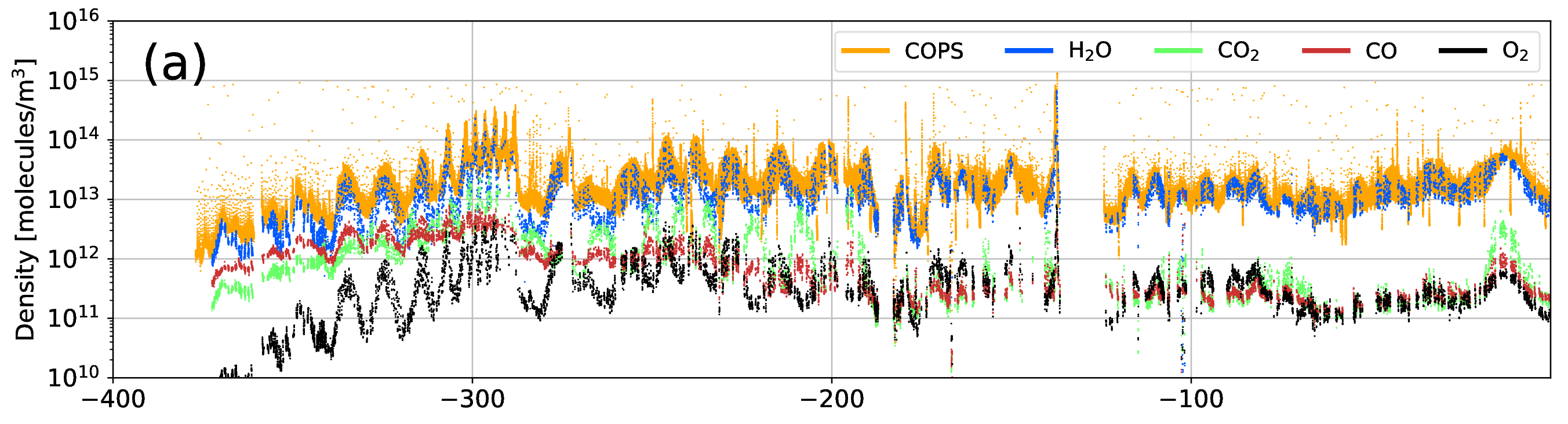
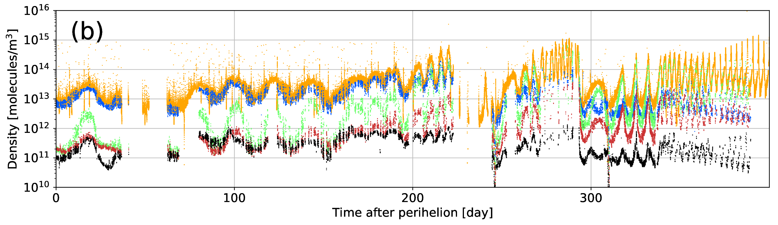
Figure 1: Observations at the positions of Rosetta, COPS data at times $T_{\mathrm{COPS}}$, DFMS data at times $T_{\mathrm{DFMS}}$, (a) time interval $(-400,0)$ days, (b) time interval $(0,400)$ days.

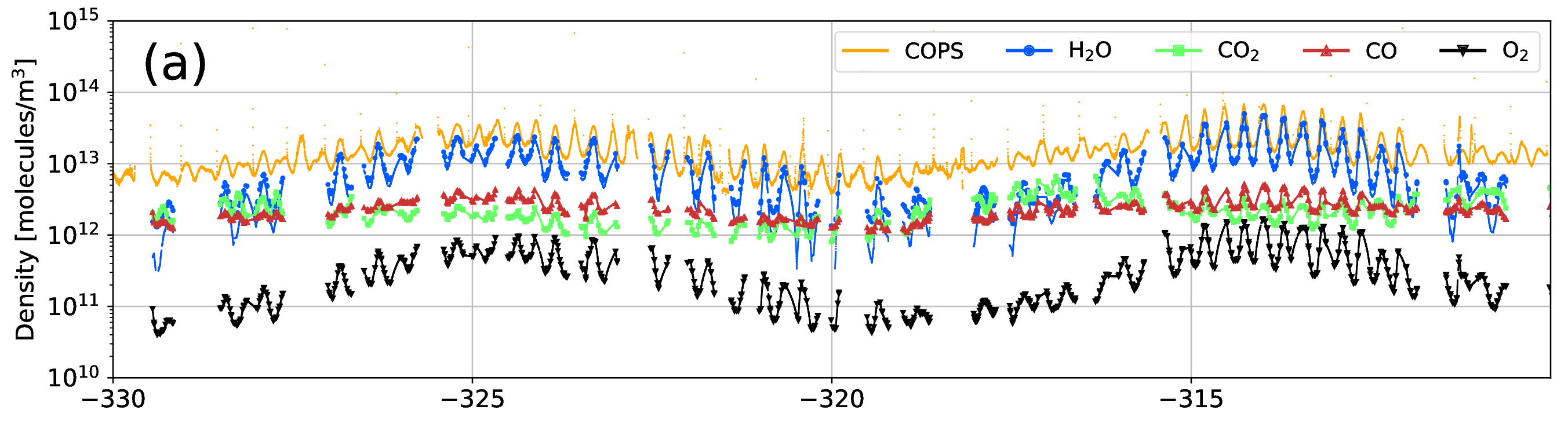
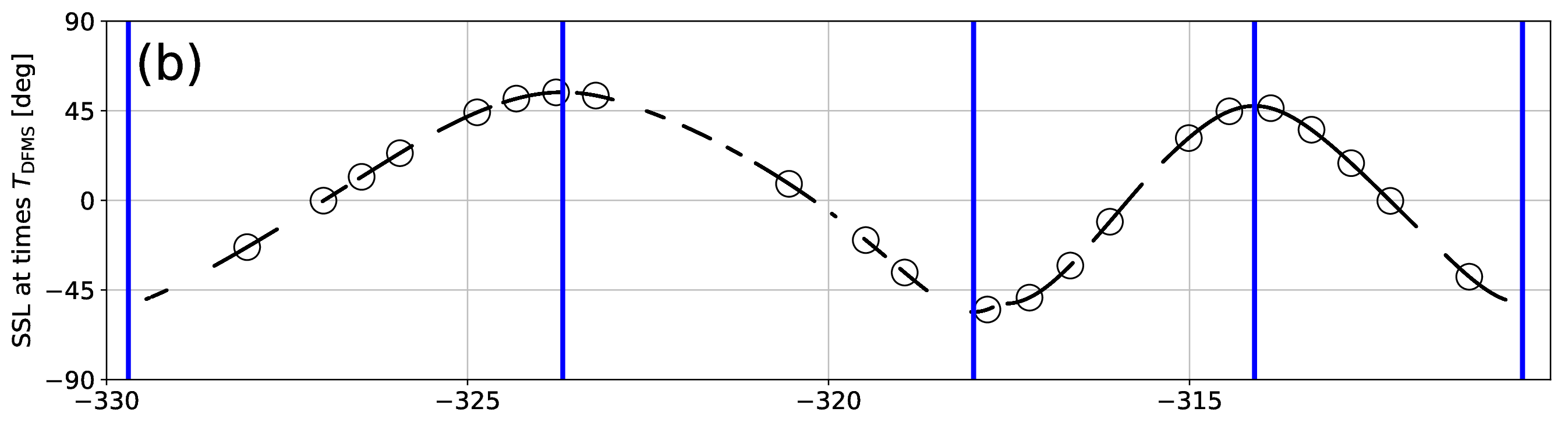
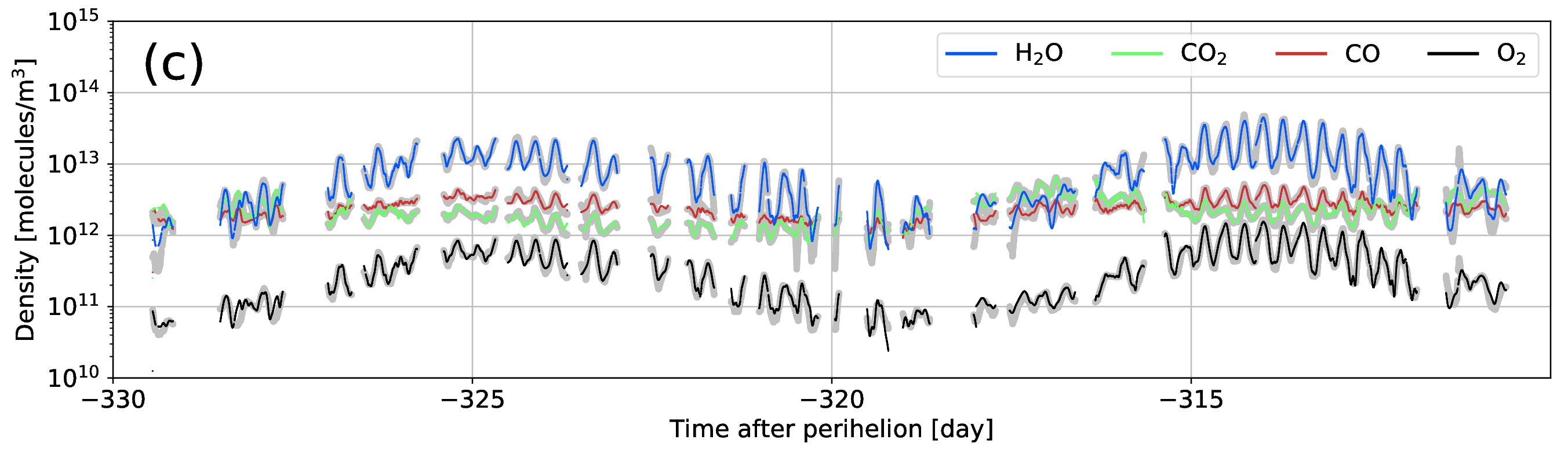
Figure 2: (a) Observations at the positions of Rosetta, COPS data at times $T_{\mathrm{COPS}}$, DFMS data at times $T_{\mathrm{DFMS}}$ (filled symbols), and DFMS data in Eq. (1) interpolated at the times $T_{4\mathrm{h}}$ (lines) in the time interval $(-330,-310)$ days. (b) sub-spacecraft latitude (SSL) at the times $T_{4\mathrm{h}}$ (lines), $0^{\circ}$-meridian crossings of the spacecraft (circles) and end points of time intervals $I_{j}$ (vertical lines). (c) Inverse model fits at times $T_{4\mathrm{h}}$, The DFMS data from (a) is plotted in gray lines, the dominant species are from top to bottom $\mathrm{H_{2}O}$, $\mathrm{CO}$, $\mathrm{CO_{2}}$, and $\mathrm{O_{2}}$ at day $-325$.

3 Reconstruction of the coma from local measurements

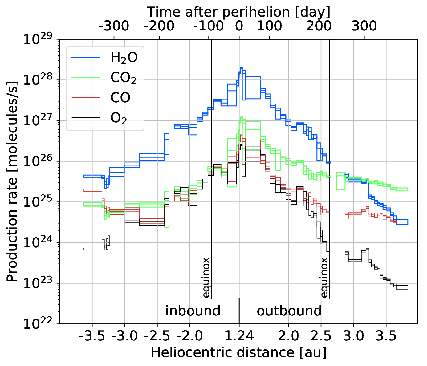
Figure 3: Production rates $Q_{s}(t)$ for the species $s=\mathrm{H_{2}O}$, $\mathrm{CO_{2}}$, $\mathrm{CO}$, and $\mathrm{O_{2}}$ over time and heliocentric distance. The boxes denote the minimum, linear and maximum estimates due to varying spacecraft surface coverage, see section 3. From top to bottom the dominant species are $\mathrm{H_{2}O}$, $\mathrm{CO_{2}}$, $\mathrm{CO}$, and $\mathrm{O_{2}}$ at outbound equinox.

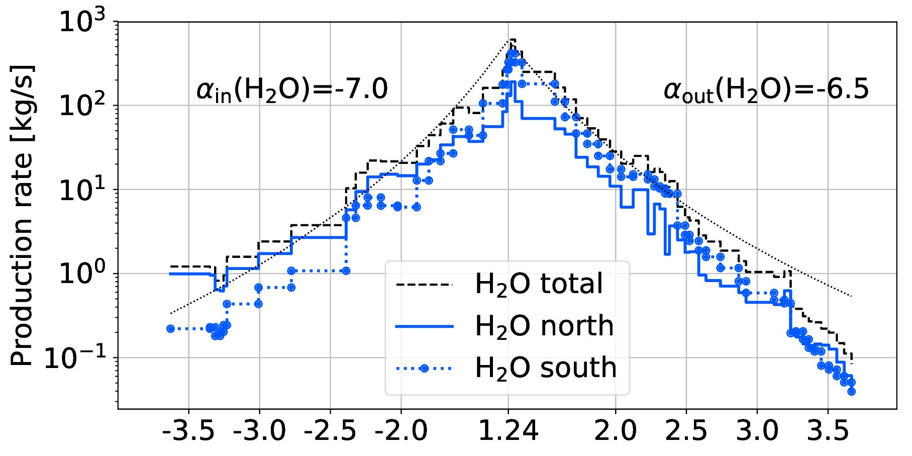
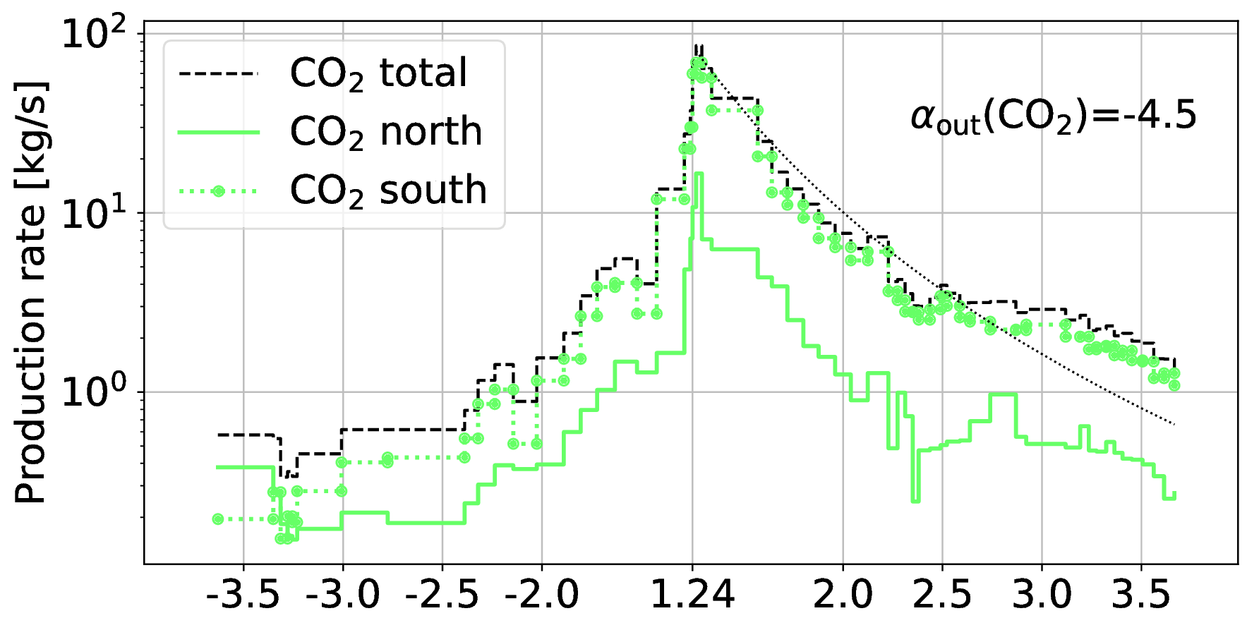
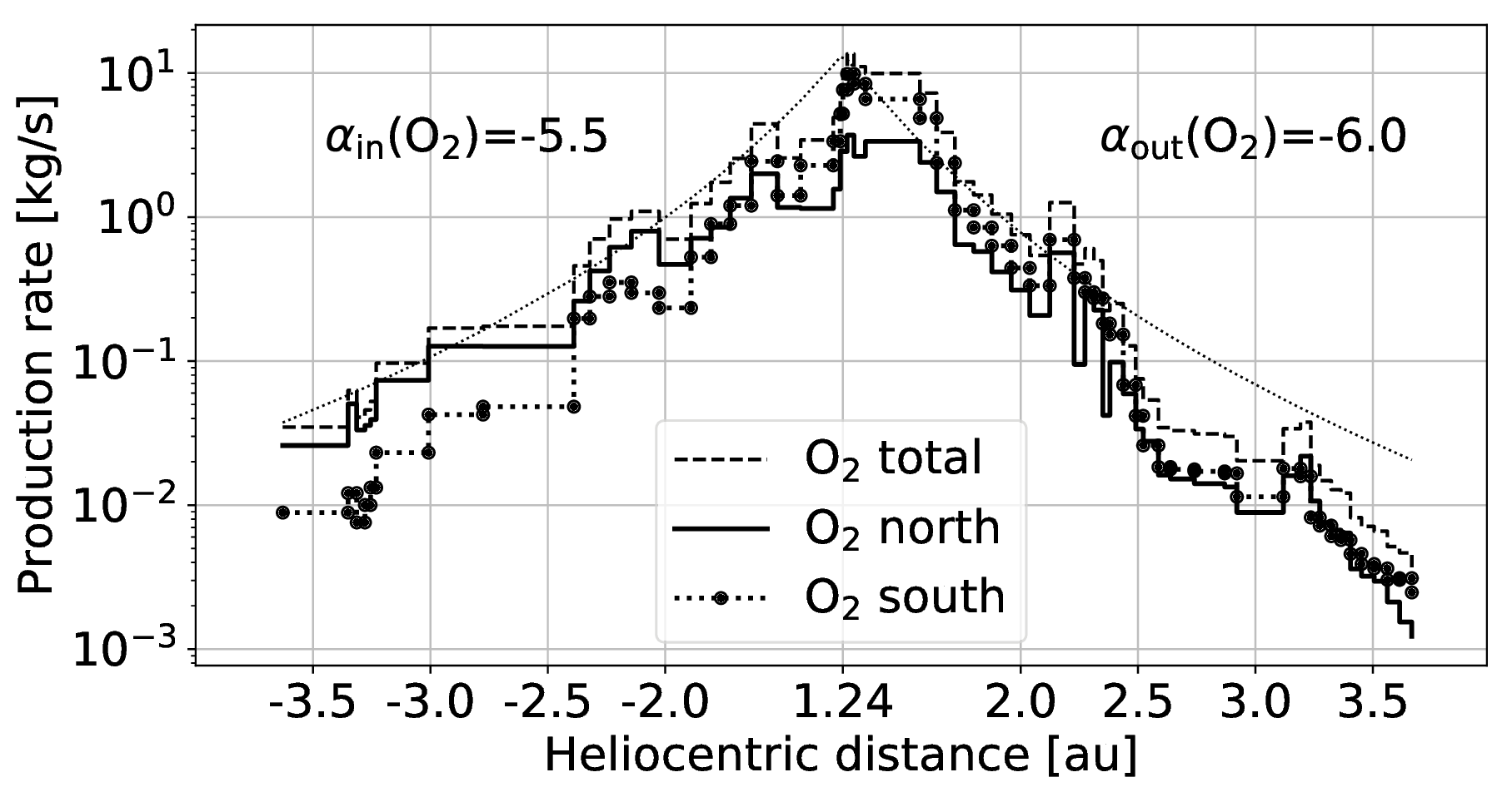
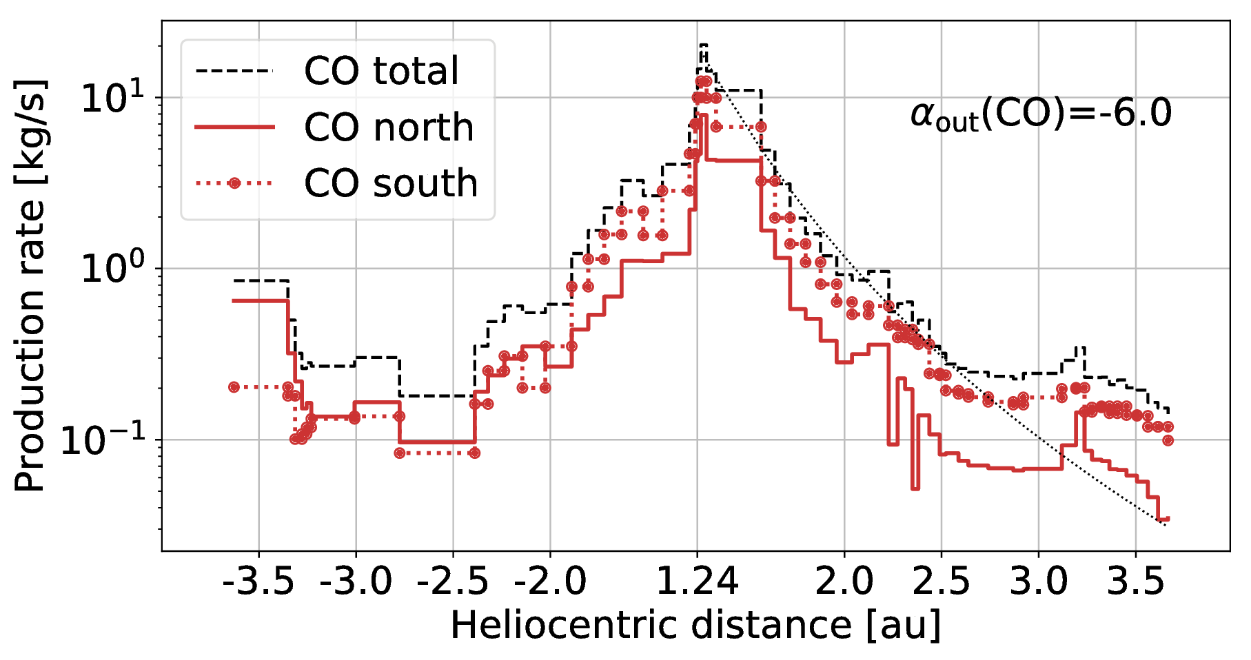
Figure 4: Production rates $Q_{s\mathrm{}}({r_{\mathrm{h}}})$ (split into northern, southern hemisphere and total) for the species $s=\mathrm{H_{2}O}$, $\mathrm{CO_{2}}$, $\mathrm{CO}$, and $\mathrm{O_{2}}$ as a function of heliocentric distance ${r_{\mathrm{h}}}$, power-law fits $Q_{s\mathrm{}}({r_{\mathrm{h}}})\sim{r_{\mathrm{h}}}^{\alpha(s)}$.

The global reconstruction of the entire three-dimensional coma around 67P/C-G proceeds as a two-step process from the time-series of COPS and DFMS measurements along the trajectory of Rosetta and is based on the assignment of surface emission rates as described by Kramer et al. (2017). First we run a forward model on a surface shape to build a global coma model by assuming equally strong emitting gas sources on each of the surface elements. In the second step we apply the inverse model and adjust the emission rates of each source to obtain the best match with the actually measured DFMS/COPS data. Systematic model uncertainties (insufficient observational sampling in space or/and time) are discussed below.

The whole surface of the nucleus is approximated by a triangular mesh with $N_{\mathrm{E}}=3996$ equidistantly spaced surface elements, leading to a spatial resolution of $110$ m on average. The original shape model SPC-ESA (2016) is remeshed using the ACDVQ tracing tool by Valette et al. (2008) and smoothed. We have validated the method by performing the model inversion for more and less detailed shape models. The surface reconstructions from higher-resolution models are slightly more scattered (see Kramer et al. (2017) for COPS data), but do not change the regional results discussed here.

To follow the evolution of the emission rates as the comet orbits the sun, we divide the complete time interval $(-372{},390{})$ days into $N_{\mathrm{I}}=58$ subintervals.

$$-372{}=t_{0},t_{1},...,t_{N_{\mathrm{I}}}=390{},$$

$$I_{j}=(t_{j-1},t_{j}),\quad\text{for}\quad j=1,...,N_{\mathrm{I}}$$

Each subinterval $I_{j}$ includes 8600 values from $T_{4\mathrm{h}}$ on average and comprises typically $14$ days. As an example, Fig. 2(b) shows four subintervals, each enclosing extremal sub-spacecraft latitudes and five or more comet rotations. Because the data points need to constrain the parameters, the complete determination of the $N_{\mathrm{E}}$ model parameters (here: the surface emission rate) requires to have more data points available (here: DFMS/COPS measurements). The intervals $I_{j}$ are chosen such that the spacecraft positions in $I_{j}$ result in an almost complete coverage of the nucleus surface. Surface sources with no flyover within the interval $I_{j}$ are set to zero emission for the lower-bound estimate of the activity.

For building the forward model, we consider the approach of Kramer et al. (2017) and introduce a model for a collisionless gas regime in the coma. Around perihelion and close to the nucleus, estimated gas densities of up to $10^{18}~{}\mathrm{molecules}/\mathrm{m}^{3}$ result in mean free paths of about $3$ m. This value is considerably larger than the mean free paths considered by Gombosi et al. (1986) (0.1-1) m, Crifo et al. (2004) ($<1$ m), and Tenishev et al. (2008) ($<1$ m) and results in higher Knudsen numbers $>0.003$. Away from perihelion and further away from the nucleus, the fast $\sim 1/r^{2}$ drop in gas density quickly leads to intermediate and collisionless flow regimes. From Fig. 2 in Finklenburg et al. (2011), we estimate the uncertainties due to collisions at observational spacecraft distances to be less than 25% around perihelion, resulting in smaller contributions to the model uncertainties compared to coverage and fitting errors.

On every surface element the model assumes a point source, which emits gas with a displaced Maxwellian velocity distribution shifted by a given mean velocity. This leads to the analytical expression Eq. (1) in Kramer et al. (2017) for the density derived by Narasimha (1962). The lateral expansion of the gas column perpendicular to the surface normal is taken into account. The modeled gas density at every space point around the nucleus arises from a superposition of all surface emitters. The accurate incorporation of the nucleus shape and the possibility to assign multiple surface locations to a single gas measurement set our model apart from a simple nadir mapping of data points. The nadir method projects each spacecraft measurement onto a single point on the surface of the nucleus.

	view from north	view from south	view from (${0,-1,0}$)	view from (${0,1,0}$)
A
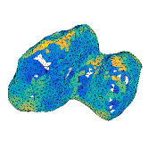
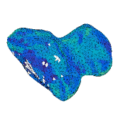
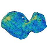
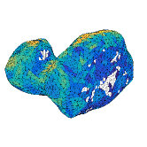
B
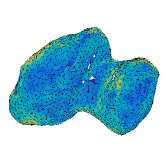
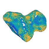
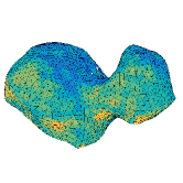
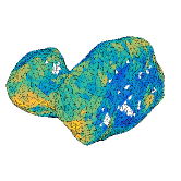
C

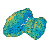
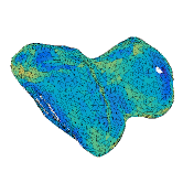
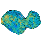
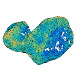
Figure 5: Surface emission rate $\dot{\rho}_{\mathrm{H_{2}O},i}$ averaged over the intervals $A=(-330,-280)$, $B=(-50,50)$, and $C=(340,390)$ days after perihelion. The colors correspond to the color bars in Fig. 7 for water and the intervals $A$, $B$, and $C$, respectively.

Within each subinterval $I_{j}$ and for every species $s=\mathrm{H_{2}O}{}$, $\mathrm{CO_{2}}{}$, $\mathrm{CO}{}$, and $\mathrm{O_{2}}{}$, the gas is emitted constantly in time. This results in an assimilation of the time-averaged surface emission rates, with a bias toward the local time of observation. A discussion of density variations due to changing sub-spacecraft longitudes follows below. The surface emission rate for each species $s$ on the surface element $i=1,...,N_{\mathrm{E}}$ is given by Eq. (4) in Kramer et al. (2017), namely

$$\dot{\rho}_{s,i}(t)=\frac{u_{s,0}}{U_{0}}q_{s,i}(I_{j}),$$

for $t\in I_{j}$ and $j=1,...,N_{\mathrm{I}}$, with the speed $u_{s,0}$ of the outflow velocity into surface normal direction and the source strength $q_{s,i}$. The emission rates are expressed in units molecules/m²/s, or alternatively rescaled to kg/m²/s with the respective molecular mass. The parameter $U_{0}$ denotes the speed ratio between the outflow velocities along the surface normal $u_{s,0}$ and into the lateral direction. We treat $U_{0}$ as an unknown parameter to be determined by a fit and set the speed into the normal direction as given in Eqs. (2) and (3). Within the exemplary test interval $(-330,-310)$ days we have compared model densities to DFMS/COPS data for different values of $U_{0}$, ranging from $U_{0}=1$ to $U_{0}=4$. A larger value $U_{0}\geq 4$ exaggerates the density variations at the sampling points, while a smaller value $U_{0}\leq 2$ diminishes the fluctuations. We have selected $U_{0}=3$, which gives the best agreement between model and observations.

The transformation of the DFMS/COPS density data to flux quantities $\dot{\rho}_{s,i}(t)$ requires to assign an outflow speed $u_{s,0}$ to the density for each interval $I_{j}$. At distances $r=10-1000$ km from the nucleus, Bockelée-Morvan & Crovisier (1987) show that the radiative equilibrium conditions in the coma lead to speeds around $850$ m/s. Lämmerzahl et al. (1988) measured $800$ m/s at $r=1000-4000$ km for comet Halley. DSMC computations by Tenishev et al. (2008) (Fig. 7) and Davidsson et al. (2010) (Figs. 2,4,5) yield speeds of water of $900-450$ m/s at heliocentric distances ${r_{\mathrm{h}}}=1.3-3.5$ au. For the choice of the speed of water we follow the approach of Hansen et al. (2016) (Tab. 1, Eq. 7, Fig. 4) and assume a function of heliocentric distance

$$u_{\mathrm{H_{2}O},0}({r_{\mathrm{h}}})=u_{\mathrm{Hansen}}({r_{\mathrm{h}}})$$ (2)

resulting in speeds between $820$ m/s and $560$ m/s. To facilitate comparisons with other models, we also consider a simplified model with a fixed water outflow speed

$$u_{\mathrm{H_{2}O},0}=755~{}\mathrm{m/s}.$$ (3)

If not stated otherwise, the results in this article are based on Eq. (2). The speeds of the other species are derived from the water speed weighted by the square root of the molecular mass ratio with water

$$u_{s,0}=u_{\mathrm{H_{2}O},0}\sqrt{\mu_{\mathrm{H_{2}O}}/\mu_{s}}.$$

The inverse model for each of the time intervals consists of a fitting process to determine all surface emission rates of the four major volatiles $\mathrm{H_{2}O}$, $\mathrm{CO_{2}}$, $\mathrm{CO}$, and $\mathrm{O_{2}}$. A typical, species-resolved density reconstruction within four intervals is shown in Fig. 2(c). Similar to Bieler et al. (2015) we observe periodic density variations (approximately two maxima per orbit around the nucleus) in the DFMS/COPS data and also for our modelled densities at the spacecraft positions. The Rosetta orbit mostly follows a terminator geometry, leading to preferential observations at morning/evening phase angles. Because our model assimilates diurnally averaged production rates within each subinterval $I_{j}$, changing illumination conditions are not resolved. The model fits are interpreted as diurnally averaged production rates of localized gas sources which reflect fluctuations due to changes of the sub-spacecraft position. This interpretation is supported by the consistent retrieval of activity spots across the entire mission from independently processed COPS/DFMS data sets taken months apart.

The model performance depends on the DFMS/COPS data distribution in time and space. In each interval $I_{j}$ the fit performance is quantified by the relative $l2$ error norm of the difference of predicted and measured densities at times $T_{4\mathrm{h}}\cap I_{j}$. All errors are in the range $0.04-0.50$, with an average value $0.16$. Possible error sources are temporal changes in surface activity or deviations from the collisionless gas model. The construction of the global emission map depends on the surface coverage of the nucleus by the spacecraft within each interval $I_{j}$. Even a limited coverage yields a subset of surface elements with known gas emission rates. We assign the source strength $q_{s,i}(I_{j})$ for an uncovered element $E_{i}$ either from a minimum, a linear, or a maximum estimate. Based on the neigboring values $l=q_{s,i}(I_{j-1})$, $r=q_{s,i}(I_{j+1})$, the minimum estimation sets $q_{s,i}(I_{j})=0$, the linear estimation sets $q_{s,i}(I_{j})$ to the average of $l$ and $r$, and the maximum estimation sets $q_{s,i}(I_{j})=\max(l,r)$. The production rates in the article are based on the linear estimate, the uncertainty values are based on the minimum and maximum estimates. The minimum estimation provides a strict lower limit, while the maximum estimation provides only a heuristic upper limit since local maxima could be dismissed. Thus, the spacecraft coverage errors could lead to an underestimation of production rates. The productions rates along with the minimum and maximum estimates are shown in Fig. 3.

4 Global gas production

$s$	$P_{s\mathrm{}}$ [molecules]	$P_{s\mathrm{}}$ [kg]	$P_{s\mathrm{,S}}/P_{s\mathrm{,N}}$	$\max Q_{s\mathrm{}}$ [kg/s]
$\mathrm{H_{2}O}$	$1.6\pm 0.5\times 10^{35}$	$4.8\pm 1.5\times 10^{9}$	$2.0$	$6.1\pm 0.3\times 10^{2}$
$\mathrm{CO_{2}}$	$9.5\pm 3.8\times 10^{33}$	$7.0\pm 2.8\times 10^{8}$	$4.9$	$8.6\pm 0.4\times 10$
$\mathrm{CO}$	$3.6\pm 1.1\times 10^{33}$	$1.7\pm 0.5\times 10^{8}$	$1.7$	$2.0\pm 0.1\times 10$
$\mathrm{O_{2}}$	$2.6\pm 0.8\times 10^{33}$	$1.4\pm 0.4\times 10^{8}$	$1.8$	$1.4\pm 0.7\times 10$

Table 1: Integrated production $P_{s\mathrm{}}$ from Eq. (4) for the species $s$, relative rates $P_{s\mathrm{,S}}/P_{s\mathrm{,N}}$ between production rates resolved by north (N) and south (S) emission location, peak production rates $\max Q_{s\mathrm{}}$.

The spatially integrated production rates $Q_{s\mathrm{}}(t)$ follow directly from the spatially and temporally resolved surface rates $\dot{\rho}_{s,i}(t)$ by summing over all $E_{i}$ shape elements

$$Q_{s\mathrm{}}(t)=\sum_{i=1}^{N_{\mathrm{I}}}\dot{\rho}_{s,i}(t)\;{\rm area}(E_{i})$$

for the gas species $s$. The integrated productions $P_{s\mathrm{}}$ in space and time during the 2015 apparition are obtained by

$$P_{s\mathrm{}}=\int_{-372~{}\mathrm{days}}^{390~{}\mathrm{days}}Q_{s}(t)\,\mathrm{d}t.$$ (4)

Similar to $\dot{\rho}_{s,i}(t)$, all production quantities depend on the molecular speeds $u_{s,0}$, see Eqs. (2),(3).

For an outflow speed depending on the heliocentric distance ${r_{\mathrm{h}}}$ (Eq. (2)), Fig. 3 shows productions rates as a function of ${r_{\mathrm{h}}}$ and of time for all species $\mathrm{H_{2}O}$, $\mathrm{CO_{2}}$, $\mathrm{CO}$, and $\mathrm{O_{2}}$. Table 1 lists the integrated productions $P_{s\mathrm{}}$ and the peak productions $\max Q_{s\mathrm{}}$. The alternative model with an overall constant outflow speed Eq. (3) leads to similar integrated production rates. The peak gas production of $2.2\pm 0.1\times 10^{28}$ molecules/s ($730\pm 30$ kg/s) is reached in the interval $I=(17,28)$ days after perihelion and is clearly dominated by $\mathrm{H_{2}O}$, whereas $\mathrm{CO_{2}}$ contributes with only one tenth of the water mass production. Compared to that, the model with constant speed (Eq. (3)) results in a reduced peak production of $2.1\pm 0.1\times 10^{28}$ molecules/s ($690\pm 30$ kg/s). For water, the peak production yields $\max Q_{\mathrm{H_{2}O}\mathrm{}}$ is $2.0\pm 0.1\times 10^{28}$ molecules/s and the integrated production $P_{\mathrm{H_{2}O}\mathrm{}}$ for one orbit yields $4.8\pm 1.5\times 10^{9}$ kg. Assuming the same outflow speed (Eq. (2)), Hansen et al. (2016) derive from COPS data a peak water production of $3.5\pm 0.5\times 10^{28}$ molecules/s $18-22$ days after perihelion. One possible reason for the higher value given by Hansen et al. (2016) might be the different interval lengths used for averaging the data (four days compared to eleven days in our case). The integrated water production of $6.4\times 10^{9}$ kg per orbit from Hansen et al. (2016) is in better agreement with our estimate. From the MIRO analysis Marshall et al. (2017) obtain a highest water emission of $1.42\pm 0.51\times 10^{28}$ molecules/s 16 days after perihelion. Their integrated water production of $2.4\pm 1.1\times 10^{9}$ kg for the apparition 2015 is half of our value. One possible cause could be a distributed source of e.g. icy grains that evaporate before reaching Rosetta where they are measured by ROSINA but do not contribute close to the nucleus to the measurements of MIRO. Another approach from Shinnaka et al. (2017) is to consider the hydrogen Lyman $\alpha$ emissions. 25 days after perihelion they obtain a water production rate of $1.46\pm 0.47\times 10^{28}$ molecules/s. The $\mathrm{H_{2}O}$ productions based on MIRO and Lyman $\alpha$ data are not peak values and thus correspond to our lower estimate.

The orbital losses allow us to constrain the dust-to-gas ratio of 67P/C-G. The total gas loss $P_{\mathrm{gas}}$ is considered to be the contributions from $\mathrm{H_{2}O}$, $\mathrm{CO_{2}}$, $\mathrm{CO}$, and $\mathrm{O_{2}}$ and further $5\%$ volatile and massive species like $\mathrm{CS_{2}}$, $\mathrm{H_{2}S}$, $\mathrm{SO_{2}}$, $\mathrm{C_{2}H_{6}}$, see Le Roy et al. (2015) and Calmonte et al. (2016). This yields $P_{\mathrm{gas}}=1.05\cdot(P_{\mathrm{H_{2}O}}+P_{\mathrm{CO_{2}}}+P_{\mathrm{CO}}+P_{\mathrm{O_{2}}})=6.1\pm 1.9\times 10^{9}$ kg and corresponds to $1/1600$ of the total mass of $M_{67P/C-G{}}=9.9778\pm 0.004\times 10^{12}$ kg from Godard et al. (2017). Considering the mass for October 2014 in Godard et al. (2015), their estimation for the total mass loss is $P_{\mathrm{dust}+\mathrm{gas}}=9\pm 6\times 10^{9}$ kg including a significant uncertainty. This uncertainty propagates to the dust-to-gas ratio of the emitted material, which we estimate to be $(P_{\mathrm{dust}+\mathrm{gas}}-P_{\mathrm{gas}})/P_{\mathrm{gas}}=0.5^{+1.1}_{-0.5}$. This value presents a lower limit for the dust-to-gas ratio. The escaping material may still contain volatiles which affect the dust-to-gas ratio, see e.g. De Keyser et al. (2017) and Altwegg et al. (2016). In addition, the dust-to-gas ratio may differ from the dust-to-ice ratio in the nucleus as backfall of dry or almost dry dust would contribute to the amount of dust ejected, but would not lead to mass loss of the nucleus.

The sufficient temporal coverage of DFMS/COPS data allows us to integrate the production per orbit by summing all interval contributions, see Eq. (4). Another possibility sometimes used in the literature is to approximate the integral from the power law fit ${r_{\mathrm{h}}}^{\alpha}$. Fig. 4 shows that the production rate $Q_{\mathrm{H_{2}O}\mathrm{}}$ follows power laws with exponents ${r_{\mathrm{h}}}^{-7}$ and ${r_{\mathrm{h}}}^{-6.5}$ for the inbound and outbound orbits, respectively. The exponents given by Hansen et al. (2016) ($-5.1\pm 0.05$ and $-7.15\pm 0.08$) and Shinnaka et al. (2017) ($-6.0\pm 0.46$ and $-5.22\pm 0.41$) are in a similar range. The data analysis of Marshall et al. (2017) yields considerably lower exponents ($-3.8\pm 0.2$ inbound, $-4.3\pm 0.2$ outbound). This is one consequence of the smaller peak production rates derived from MIRO versus ROSINA as discussed above in the context of the peak production. Although not as steep as for $\mathrm{H_{2}O}$, the $\mathrm{O_{2}}$ curves are fitted by exponents of $-5.5$ and $-6$. The inbound production of $\mathrm{CO_{2}}$ and $\mathrm{CO}$ is not well reproduced by a power law, since $150$ days before perihelion and even earlier the production rate stagnates. Outbound, the $\mathrm{CO_{2}}$ production drops down with ${r_{\mathrm{h}}}^{-4.5}$, slower than for $\mathrm{H_{2}O}$. This difference leads to a crossover from a water dominated coma to a carbon dioxide dominated one at $2.75$ au ($250$ days after perihelion). $\mathrm{CO}$ partially resembles the $\mathrm{CO_{2}}$ trend with a similar exponent ${r_{\mathrm{h}}}^{-6.0}$.

Fig. 4 and Table 1 show production contributions separated for the Northern (N) and Southern (S) hemispheres. All species are released in higher quantities from the southern hemisphere compared to the northern one. This is caused by the stronger illumination of the southern latitudes during perihelion, with summer solstice occurring only 23 days after perihelion. The asymmetric mass production ratios $P_{s\mathrm{,S}}/P_{s\mathrm{,N}}$ for $\mathrm{H_{2}O}$, $\mathrm{CO}$, and $\mathrm{O_{2}}$ range between $1.7:1$ to $2.0:1$. In contrast to that, the S/N ratio for $\mathrm{CO_{2}}$ becomes $4.9:1$. This indicates a predominant $\mathrm{CO_{2}}$ production from southern sources. In agreement with the southwards shifted integrated productions, the ratios $Q_{s\mathrm{,S}}(t)/Q_{s\mathrm{,N}}(t)$ around perihelion are close to the S/N ratios in Table 1 for $P_{s\mathrm{}}$. For $\mathrm{CO}$, the S/N ratio remains elevated also on the outbound cometary orbit after perihelion and for $\mathrm{CO_{2}}$ at almost all times. For $\mathrm{CO_{2}}$, only the first interval is an exception, where the sub-spacecraft latitude leads to a poor southern coverage.

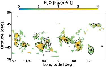
Figure 6: Surface emission rates $\dot{\rho}_{\mathrm{H_{2}O},i}$ in the time interval $B=(-50,50)$ days on the most active surface elements, contributing to 50% of the total emission; nine $\mathrm{H_{2}O}$ activity areas are marked by ovals. The circles show the positions of reported short living outbursts by Vincent et al. (2016).

A
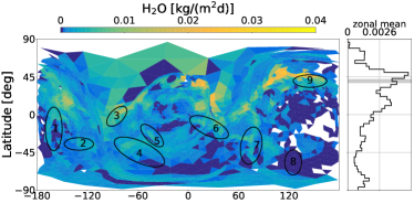
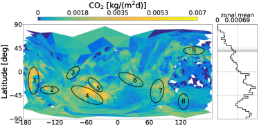
B
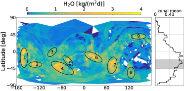
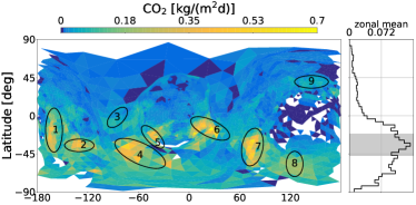
C

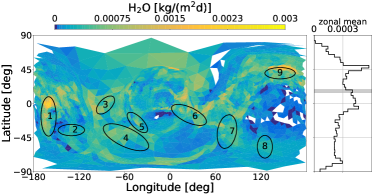
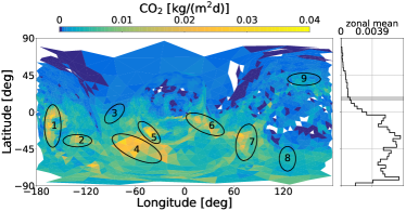
Figure 7: Surface emission rates $\dot{\rho}_{\mathrm{H_{2}O},i}$ and $\dot{\rho}_{\mathrm{CO_{2}},i}$ in the intervals $A=(-330,-280)$, $B=(-50,50)$, and $C=(340,390)$ days after perihelion. The side panels show the longitudinally averaged rate (zonal mean), the grey bar indicates the sub-solar latitude.

A
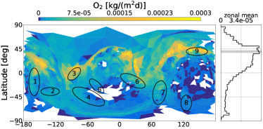
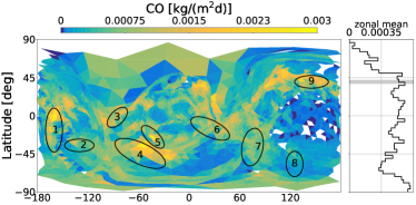
B
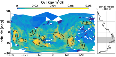
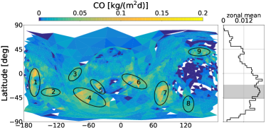
C

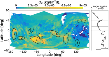
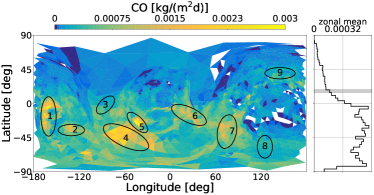
Figure 8: Surface emission rates $\dot{\rho}_{\mathrm{O_{2}},i}$ and $\dot{\rho}_{\mathrm{CO},i}$ in the intervals $A=(-330,-280)$, $B=(-50,50)$, and $C=(340,390)$ days after perihelion. The side panels show the longitudinally averaged rate (zonal mean), the grey bar indicates the sub-solar latitude.

5 Localized surface sources

It has been recognized, see e.g. Bieler et al. (2015), that a homogeneous distriubtion of the activity cannot explain the coma gas distribution. Consequently advanced models use different heterogeneous distributions of active areas. E.g. Fougere et al. (2016a) use an inverse approach for spherical harmonics in the neck region to introduce heterogeneity, Marschall et al. (2017) use specific surface morphology (cliffs, plains) to attribute activities to different areas. Our inverse model allows one to trace back in situ DFMS/COPS measurements in the coma to localized emission rates. It incorporates the complex shape of the nucleus with two lobes, large concave areas, and additional valleys, cliffs, and plains. No assumptions for the active areas on the surface of 67P/C-G enter our model.

The surface is shown from different viewing directions in Fig. 5 and colored by the surface emission rate $\dot{\rho}_{\mathrm{H_{2}O},i}$ temporally averaged over three intervals, respectively. The first interval $A=(-330,-280)$ ends months before perihelion, the second interval $B=(-50,50)$ covers the time around perihelion, and the last interval $C=(340,390)$ begins months after perihelion. According to Fig. 4 the dominating hemisphere for the $\mathrm{H_{2}O}$ emissions changes from north in interval $A$ to south in interval $B$ and back to north in interval $C$.

The integrated $\mathrm{H_{2}O}$ production over the complete interval $(-372{},390{})$ amounts to $780\pm 250$ kg/m² in the most active source regions and to $110\pm 30$ kg/m² on average. Assuming a pure water ice surface with a density of $470$ kg/m³, this corresponds to a maximum ice erosion of $1.7$ m. The average ice erosion across the entire nucleus and orbit is then $0.23$ m. With increasing dust-to-gas ratio the erosion height increases correspondingly.

To focus the discussion to regions of highest activity, Fig. 6 shows the most abundant volatile $\mathrm{H_{2}O}$ around perihelion in the latitude/longitude Cheops-frame defined by Preusker et al. (2015). Only those surface elements are depicted that contribute 50% of the total water loss during the time interval $B$. Based on this set nine oval activity areas are marked. Area 1 covers parts of the regions Apis and Khonsu, area 3 parts of the region Anuket, area 6 parts of the region Bastet, area 7 parts of the region Bes and Khepry, area 8 parts of the region Bes and area 9 parts of the region Ash (see Fig. 11 of El-Maarry et al. (2016) for the definition of regions). Our activity areas contain 23 out of 34 locations of short living outbursts around perihelion (small circles) reported by Vincent et al. (2016). This remarkable correlation is even more pronounced and longer lasting (including months before and after perihelion) in the $\mathrm{CO_{2}}$ data discussed below.

The attached side panels to Figs. 7 and 8 show the longitudinally averaged emission (zonal mean) and in addition indicate the range of sub-solar latitudes during the considered interval. Around perihelion and southern solstice (in interval $B$), all emission peaks are concentrated on the southern hemisphere close to the sub-solar latitude at that time. Months before inbound equinox (in interval $A$), the peaks for $\mathrm{H_{2}O}$ and $\mathrm{O_{2}}$ are also linked to the sub-solar latitude in the north. Months after outbound equinox (in interval $C$), $\mathrm{H_{2}O}$ and $\mathrm{O_{2}}$ feature peaks near the northern sub-solar latitude but still have contributions from the southern hemisphere. In contrast to $\mathrm{H_{2}O}$ and $\mathrm{O_{2}}$, the peaks for the volatiles $\mathrm{CO_{2}}$ and $\mathrm{CO}$ are decoupled from the sub-solar latitude in the intervals $A$ and $C$. Substantial emissions originate from the southern hemisphere. The strongest $\mathrm{CO_{2}}$ sources remain localized on the southern hemisphere for all intervals independent to the corresponding sub-solar latitude.

Figs. 7 and 8 show the overall surface emissions averaged within the time intervals $A$, $B$, and $C$ for all species $\mathrm{H_{2}O}$, $\mathrm{CO_{2}}$, $\mathrm{CO}$, and $\mathrm{O_{2}}$. For $\mathrm{H_{2}O}$ this corresponds to the three-dimensional representation in Fig. 5. The seasonally changing solar illumination leads to latitudinal shifts in the source distribution, but with different patterns for $\mathrm{H_{2}O}$, $\mathrm{CO_{2}}$, $\mathrm{CO}$, and $\mathrm{O_{2}}$. Peak sources for $\mathrm{H_{2}O}$, $\mathrm{CO_{2}}$, and $\mathrm{CO}$ appear roughly at places in agreement to Hoang et al. (2017) who projected the RTOF density measurements to a $10$ km surface. This agreement becomes even better when comparing the RTOF data for $\mathrm{H_{2}O}$ with Fig. 4 in Kramer et al. (2017), which shows our inverse model data on a $100$ km surface. As suggested by VIRTIS-H observations in Bockelée-Morvan et al. (2016), by modeling results in Fougere et al. (2016b) and Hoang et al. (2017), $\mathrm{CO_{2}}$, $\mathrm{CO}$ are decoupled from $\mathrm{H_{2}O}$ at the time before inbound equinox. This matches our observation in interval $A$, that $\mathrm{CO_{2}}$ and $\mathrm{CO}$ are mainly located in the southern hemisphere, while $\mathrm{H_{2}O}$ originates from the northern hemisphere.

Around perihelion (in interval $B$) the $\mathrm{H_{2}O}$ emissions are not limited to the nine activity areas but occur to some extent around the entire nucleus. $\mathrm{CO}$ and $\mathrm{O_{2}}$ are predominantly active in all water areas, but $\mathrm{CO_{2}}$ coincides with water only for the southern areas 1-2, 4-8. On the northern hemisphere, the $\mathrm{CO_{2}}$ emission is almost absent from area 3, close to the Anuket fracture described in El-Maarry et al. (2015), and area 9 in the Ash region. Area 7 covers the patches reported by Filacchione et al. (2016) and Fornasier et al. (2016) including high $\mathrm{CO_{2}}$ ice and $\mathrm{H_{2}O}$ ice concentrations around day $-145$ and around day $-105$, respectively. Although their observations are made before our interval $B$, the agreement for this source localization is still remarkable.

During the inbound northern summer (in interval $A$) $\mathrm{H_{2}O}$ and $\mathrm{O_{2}}$ activity is located along a northern belt including the areas 3, 6, and 9. This repeats in the outbound northern summer (in interval $C$) and is complemented by activity in southern areas 1, 4, and 6 for $\mathrm{H_{2}O}$ and in 1-2, 4-5, 7-8 for $\mathrm{O_{2}}$. Thus, $\mathrm{O_{2}}$ source locations correlate to $\mathrm{H_{2}O}$ source locations during all intervals $A$, $B$, and $C$. For the inbound northern summer (in interval $A$) $\mathrm{CO_{2}}$ and $\mathrm{CO}$ activity is widely spread over the whole surface, $\mathrm{CO_{2}}$ exhibits important contributions from the southern areas 1-2, 4-8, almost all activity areas (except area 8) show $\mathrm{CO}$ emissions. Comparing this pattern to $\mathrm{H_{2}O}$ sources, $\mathrm{CO}$ sources seem to correlate to a linear combination of $\mathrm{H_{2}O}$ and $\mathrm{CO_{2}}$ sources. At the same time despite the low emission from area 8, $\mathrm{CO_{2}}$ emissions in area 8 and surroundings in region Imhotep are still higher than the $\mathrm{H_{2}O}$ emissions. This shows a good agreement to the area of high ratio $\rho_{\mathrm{CO_{2}}}/\rho_{\mathrm{H_{2}O}}$ described in Hässig et al. (2015). During outbound northern summer, when $Q_{\mathrm{H_{2}O}\mathrm{}}$ is almost vanished, the pattern of $\mathrm{CO}$ sources seem to correlate to $\mathrm{CO_{2}}$ sources only. Both source patterns focus to the southern areas 1-2, 4-8.

The $\mathrm{CO_{2}}$ sources are pinned to the south throughout the whole Rosetta mission at the marked active areas: for all intervals $A$, $B$, and $C$ the southern $\mathrm{CO_{2}}$ sources (areas 1-2, 4-8) remain active. This shows the consistent retrieval and assignment of $\mathrm{CO_{2}}$ sources for the intervals $A$ and $C$, long before and after perihelion, respectively. Because these surface locations are reconstructed from completely disjunct data sets and widely varying spacecraft trajectories, this validates our inverse model approach. Furthermore, the location of $\mathrm{CO_{2}}$ sources on the southern hemisphere is in agreement with the COPS data analysis for the month May 2016 performed in Kramer et al. (2017).

6 Discussion

In this manuscript, we have presented emission rates for the gas species $\mathrm{H_{2}O}$, $\mathrm{CO_{2}}$, $\mathrm{CO}$, and $\mathrm{O_{2}}$ with high spatial resolution on the surface of 67P/C-G and also temporally resolved in the time between August 6th 2014 and September 5th 2016. Previous surface maps were derived from lower resolution expansions with 25 parameters by Fougere et al. (2016b) and did not localize gas sources due to the inherent averaging over longitudes. The coma model by Marschall et al. (2017) considers various topographical features as gas sources, does not employ an inversion process, and leads to a non-unique source attribution. The lower longitudinal resolution of the inversion models by Hansen et al. (2016) (Fig. 10) and Fougere et al. (2016b) (Fig. 5) results in striped activity patterns and concentric fringes around the poles, respectively. With the 100 fold increase of resolution shown here, we obtain a more accurate determination of local gas emitters on the surface, validated by matching with independent optical observations of outbreaks and spectroscopy of icy patches. Another internal consistency check of the model is the assignment of identical gas sources across completely distinct time-periods with vastly varying solar radiation and spacecraft orbits. In contrast to previous inversions, which work with single data sets covering a long interval (300 days by Fougere et al. (2016a)), the combined COPS/DFMS data set allows us to trace the coma evolution in 14 days intervals. We also introduced a systematic uncertainty quantification due to missing visibility of surface areas. The reconstruction was based on the inverse gas model in Kramer et al. (2017) and in situ DFMS/COPS measurements in the coma. Based on the speed assumption in Hansen et al. (2016) for each of the species, peak production rates (integrated over space) and integrated (over space and time) productions rates are evaluated. The summation over all gas species yields a peak production rate $2.2\pm 0.1\times 10^{28}$ molecules/s, an integrated production rate $5.8\pm 1.8\times 10^{9}$ kg, and a maximum (averaged) water ice erosion of $1.7$ m ($0.23$ m). Incorporating the total mass loss, for the dust-to-gas ratio this yields $0.5^{+1.1}_{-0.5}$.

Nine activity areas are defined by $\mathrm{H_{2}O}$ emissions around perihelion and those correlate well with short living outbursts reported by Vincent et al. (2016). The examination of the nine areas before, around, and after perihelion shows that the source locations of $\mathrm{H_{2}O}$ and $\mathrm{O_{2}}$ follow the sub-solar latitude and correlate to each other. In contrast to that, $\mathrm{CO_{2}}$ sources are mainly located in southern areas throughout the whole mission. $\mathrm{CO}$ correlates to a linear combination of $\mathrm{H_{2}O}$ and $\mathrm{CO_{2}}$ months before inbound equinox, months after outbound equinox it correlates to $\mathrm{CO_{2}}$ only.

By comparing optical observations with dust-coma models (Kramer & Noack (2015); Kramer et al. (2018)) it is known that the dust coma is best explained by a uniform activity across the entire sunlit nucleus, which points to a rather homogeneous surface composition.

The surface localization of emissions for different gas species, also described by A’Hearn et al. (2011) for comet Hartley 2, is a first step to connect observational data to the reconstruction with first-principle modeling of cometary activity such as suggested by Keller et al. (2015). The fast drop of the water production rates with increasing heliocentric distance rules out the simplest sublimation models from Keller et al. (2015) taking a uniformly covered icy body with $Q_{\mathrm{H_{2}O}\mathrm{}}\sim{r_{\mathrm{h}}}^{-2.8}$ in model A. One way to accommodate higher exponents in the power law is to consider a time-varying dust-cover on the surface, leading to a transition from Keller model A to models with larger dust cover. In addition, the peak water production of $\sim 3200$ kg/s in model A (a completely water ice covered surface) is about five times as high as our peak production. A detailed comparison with first principle thermal and compositional models of the surface is planned for future work.

References

- A’Hearn et al. (2011) A’Hearn M. F., et al., 2011, Science, 332, 1396
- Altwegg et al. (2016) Altwegg K., et al., 2016, Science Advances, 2
- Balsiger et al. (2007) Balsiger H., et al., 2007, Space Science Reviews, 128, 745
- Bieler et al. (2015) Bieler A., et al., 2015, Astronomy & Astrophysics, 583, A7
- Bockelée-Morvan & Crovisier (1987) Bockelée-Morvan D., Crovisier J., 1987, in Proceedings of the International Symposium on the Diversity and Similarity of Comets. pp 235–240
- Bockelée-Morvan et al. (2016) Bockelée-Morvan D., et al., 2016, Monthly Notices of the Royal Astronomical Society, 462, S170
- Calmonte et al. (2016) Calmonte U., et al., 2016, Monthly Notices of the Royal Astronomical Society, 462, S253
- Crifo et al. (2004) Crifo J., Fulle M., Kömle N. I., Szego K., 2004, Comets II, pp 471–504
- Davidsson et al. (2010) Davidsson B. J., Gulkis S., Alexander C., von Allmen P., Kamp L., Lee S., Warell J., 2010, Icarus, 210, 455
- De Keyser et al. (2017) De Keyser J., et al., 2017, Monthly Notices of the Royal Astronomical Society, 469, S695
- El-Maarry et al. (2015) El-Maarry M. R., et al., 2015, Geophysical Research Letters, 42, 5170
- El-Maarry et al. (2016) El-Maarry M. R., et al., 2016, Astronomy & Astrophysics, 593, A110
- Filacchione et al. (2016) Filacchione G., et al., 2016, Science, 354, 1563
- Finklenburg et al. (2011) Finklenburg S., Thomas N., Knollenberg J., Kührt E., 2011, in AIP Conference Proceedings. p. 1151
- Fornasier et al. (2016) Fornasier S., et al., 2016, Science, 354, 1566
- Fougere et al. (2016a) Fougere N., et al., 2016a, Monthly Notices of the Royal Astronomical Society, 462, S156
- Fougere et al. (2016b) Fougere N., et al., 2016b, Astronomy & Astrophysics, 588, A134
- Gasc et al. (2017) Gasc S., et al., 2017, Planetary and Space Science, 135, 64
- Godard et al. (2015) Godard B., Budnik F., Muñoz P., Morley T., Janarthanan V., 2015, Proceedings 25th International Symposium on Space Flight Dynamics, Munich, Germany
- Godard et al. (2017) Godard B., Budnik F., Bellei G., Morley T., 2017, in International Symposium on Space Flight Dynamics-26th ISSFD. Matsuyama, Japan
- Gombosi et al. (1986) Gombosi T. I., Nagy A. F., Cravens T. E., 1986, Reviews of Geophysics, 24, 667
- Hansen et al. (2016) Hansen K. C., et al., 2016, Monthly Notices of the Royal Astronomical Society, 15, stw2413
- Haser (1957) Haser L., 1957, Bulletin de la Class des Sciences de l’Académie Royale de Belgique, 43, 740
- Hässig et al. (2015) Hässig M., et al., 2015, Science, 347, aaa0276
- Hoang et al. (2017) Hoang M., et al., 2017, Astronomy & Astrophysics, 600, A77
- Keller et al. (2015) Keller H. U., et al., 2015, Astronomy & Astrophysics, 583, A34
- Kramer & Noack (2015) Kramer T., Noack M., 2015, The Astrophysical Journal, 813, L33
- Kramer et al. (2017) Kramer T., Läuter M., Rubin M., Altwegg K., 2017, Monthly Notices of the Royal Astronomical Society, 469, S20
- Kramer et al. (2018) Kramer T., Noack M., Baum D., Hege H.-C., Heller E. J., 2018, Advances in Physics: X, 3, 1404436
- Lämmerzahl et al. (1988) Lämmerzahl P., et al., 1988, Exploration of Halley’s Comet, pp 169–173
- Le Roy et al. (2015) Le Roy L., et al., 2015, Astronomy & Astrophysics, 583, A1
- Marschall et al. (2016) Marschall R., et al., 2016, Astronomy & Astrophysics, 589, A90
- Marschall et al. (2017) Marschall R., et al., 2017, Astronomy & Astrophysics, 605, A112
- Marshall et al. (2017) Marshall D. W., et al., 2017, Astronomy & Astrophysics, 603, A87
- Narasimha (1962) Narasimha R., 1962, Journal of Fluid Mechanics, 12, 294
- Preusker et al. (2015) Preusker F., et al., 2015, Astronomy & Astrophysics, 583, A33
- SPC-ESA (2016) SPC-ESA 2016, ESA/RMOC, SPC-ESA MTP019 cartesian plate model low res dsk for comet 67P/C-G, https://pdssbn.astro.umd.edu/holdings/ro-c-multi-5-67p-shape-v2.0/data/spice_dsk/spc_esa/mtp019/cshp_dv_130_01_lores_bds.lbl
- Schroeder et al. (2018) Schroeder I. R., et al., 2018, Astronomy & Astrophysics
- Schulz (2009) Schulz R., 2009, Solar System Research, 43, 343
- Shinnaka et al. (2017) Shinnaka Y., et al., 2017, The Astronomical Journal, 153, 76
- Tenishev et al. (2008) Tenishev V., Combi M., Davidsson B., 2008, The Astrophysical Journal, 685, 659
- Valette et al. (2008) Valette S., Chassery J.-M., Prost R., 2008, IEEE Transactions on Visualization and Computer Graphics, 14, 369
- Vincent et al. (2016) Vincent J.-B., et al., 2016, Monthly Notices of the Royal Astronomical Society, 462, S184