Contact interactions and Kronig-Penney Models in Hermitian and ${\cal PT}$ symmetric Quantum Mechanics

Abstract

The delta function potential is a simple model of zero-range contact interaction in non-relativistic quantum mechanics in one dimension. The Krönig-Penney model is a one-dimensional periodic array of delta functions and provides a simple illustration of energy bands in a crystal. Here we investigate contact interactions that generalize the delta function potential and corresponding generalizations of the Krönig-Penney model within conventional and ${\cal PT}$ symmetric quantum mechanics. In conventional Hermitian quantum mechanics we determine the most general contact interaction compatible with self-adjointness and in ${\cal PT}$ quantum mechanics we consider interactions that respect symmetry under the transformation ${\cal PT}$ where ${\cal P}$ denotes parity and ${\cal T}$ denotes time reversal. In both cases we find that the most general interaction has four independent real parameters and depending on the values of those parameters the contact interaction can support zero, one or two bound states. By contrast the conventional delta function can only support zero or one bound state. In the ${\cal PT}$ symmetric case moreover the two bound state energies can be both real or a complex conjugate pair. The transition from real to complex bound state energies corresponds to the spontaneous breaking of ${\cal PT}$ symmetry. The scattering states for the ${\cal PT}$ symmetric case are also found to exhibit spontaneous breaking of ${\cal PT}$ symmetry wherein the eigenvalues of the non-unitary S- matrix depart the unit circle in the complex plane. We also investigate the energy bands when the generalized contact interactions are repeated periodically in space in one dimension. In the hermitian case we find that the two bound states result in two narrow bands generically separated by a gap. These bands intersect at a single point in the Brillouin zone as the interaction parameters are varied. Near the intersection the bands form a massless Dirac cone. In the ${\cal PT}$ symmetric case we find that as the parameters of the contact interaction are varied the two bound state bands undergo a ${\cal PT}$ symmetry breaking transition wherein the two band energies go from being real to being a complex conjugate pair. The ${\cal PT}$ symmetric Krönig- Penney model provides a simple soluble example of the transition which has the same form as in other models of ${\cal PT}$ symmetric crystals.

I Introduction

A fundamental principle of quantum mechanics is that operators which correspond to observable quantities, most notably, the Hamiltonian, must be Hermitian hermiticity . Recently there has been a surge of interest in operators that are non-hermitian but respect the combined symmetry ${\cal PT}$ where ${\cal P}$ denotes parity and ${\cal T}$ is time reversal benderprl ; benderrev . In classical optics it has proved possible to fabricate materials with alternating regions of gain and loss that demonstrate many novel optical properties (for recent reviews see photo1 ; photo2 ). In such systems the equation that governs the propagation of electromagnetic waves can be engineered to have the form of a Schrödinger equation with ${\cal PT}$ symmetry. In order to build intuition for wave propagation in these materials it is therefore relevant to consider simple models of ${\cal PT}$ quantum mechanics. In this paper we construct the ${\cal PT}$-symmetric generalizations of two models well-known from conventional Hermitian quantum mechanics: the delta function potential and the simplest model of a periodic crystal, the Krönig-Penney model.

The delta function is a widely used model of a zero-range contact interaction in quantum mechanics. Rigorously it is a viable model of contact interaction only in one dimension. In higher dimensions the ideal delta function potential is invisible and it is better to treat contact interactions as modified boundary conditions jackiw . Here we show that even in one dimension it is helpful to model a contact interaction as a boundary condition; adopting this point of view we find that even in hermitian quantum mechanics in one dimension the delta function is merely a special case of the most general allowed contact interaction. Quite different forms of contact interaction emerge when we relax the conditions of hermitian self-adjointness but instead impose the requirement of ${\cal PT}$ symmetry. We find that for both the hermitian and ${\cal PT}$ symmetric generalized contact interactions there can be zero, one or two bound states depending on the parameters that characterize the interaction. In contrast the conventional delta function can only have zero or one bound states depending on whether the the potential is attractive or repulsive. In the ${\cal PT}$ symmetric case when there are two bound states the eigenvalues can be either both real or a complex conjugate pair depending on the parameters of the model. As the parameters pass through a critical value, the real eigenvalues degenerate and enter the complex plane, behavior that is called the ${\cal PT}$ transition benderrev . The ${\cal PT}$ transition is accompanied by spontaneous breaking of ${\cal PT}$ symmetry: although the interaction remains ${\cal PT}$ symmetric, the eigenstates are no longer invariant under ${\cal PT}$. We also identify a ${\cal PT}$ transition in the scattering states. In this case the energy is necessarily real; the transition occurs when the eigenvalues of the non-unitary $S$-matrix cease to be unimodular and depart from the unit circle in the complex plane doug .

We generalize the conventional Krönig-Penney model by considering a periodic array of generalized contact interactions in one dimension. In the hermitian case the two bound state bands have a simple cosine dispersion when they are well separated. However when the parameters of the contact interaction are tuned suitably the bands intersect at an isolated point in the Brillouin zone. Near the intersection the band structure is a massless Dirac cone. This behavior is reminiscent of topological insulators where gap closure is a phase boundary that separates an ordinary insulator from a topological insulator kane . Whether that is the case here is a question we leave open for future work. For the ${\cal PT}$ symmetric case the two bound state bands undergo a ${\cal PT}$ symmetry breaking transition as the parameters are varied (see fig 2). Before the onset of the transition the two bands are entirely real. After the transition is complete the bands are a complex conjugate pair. For intermediate values of the parameters the bands are real over part of the Brillouin zone and a conjugate pair over the remainder. The ${\cal PT}$ symmetric Krönig-Penney model thus constitutes a particularly simple and soluble model that exhibits these generic features of ${\cal PT}$ symmetric crystals. The generalized hermitian Krönig-Penney model may be useful as a description of semiconductor superlattices davies and the ${\cal PT}$ symmetric generalization may be relevant to experiments in ${\cal PT}$ optics photo1 ; photo2 .

Boundary conditions that respect ${\cal PT}$ symmetry were first introduced by Krejcirik et al. in context of a particle in a box and generalizations thereof in a series of papers krejcirik1 ; krejcirik2 ; krejcirik3 ; krejcirik4 ; krejcirik5 ; see also dasarthy . The study of periodic ${\cal PT}$ symmetric potentials was initiated by ref benderperiod ; jones ; ahmed . Subsequently ref creol spurred experimental activity in the field by identifying practical realizations in optics and by discovering novel wave propagation effects in crystals with ${\cal PT}$ symmetry. The work of refs jones ; ahmed is particularly closely related to the present work. These authors introduced and analyzed a version of the Krönig-Penney model wherein the periodic potential is piecewise constant. Here by contrast we consider a different Krönig-Penney model that consists of repetitions of zero range contact interactions that cannot be obtained from the models of refs jones ; ahmed by any limiting procedure. Motivated by very different considerations of topology change, quantum gravity and many-worlds quantum mechanics the authors of ref wilczek have also considered hermitian generalizations of the contact interaction. We discuss the relationship of our results to ref wilczek in section II.1.

II Contact Interaction

Consider the textbook problem of a non-relativistic particle of mass $m$ in one dimension interacting with a delta function potential $\lambda\delta(x)$ located at the origin. Rather than treating the delta function as a potential we may regard it as a boundary condition that the wave function must satisfy, namely, continuity at the origin, $\psi(0^{+})=\psi(0^{-})$, and discontinuity in the derivative given by

$$\psi^{\prime}(0^{+})=\frac{2m\lambda}{\hbar^{2}}\psi(0^{-})+\psi^{\prime}(0^{-}).$$ (1)

Viewing the delta function as a boundary condition suggests a more general model of a contact interaction wherein the wavefunction satisfies the boundary condition

$$\psi(0^{+}) = a\psi(0^{-})+b\psi^{\prime}(0^{-})$$

$$\psi^{\prime}(0^{+}) = c\psi(0^{-})+d\psi^{\prime}(0^{-})$$ (2)

where $a,b,c$ and $d$ are complex constants. This is the most general boundary condition compatible with linearity and the order of the Schrödinger equation. The conventional delta function is the special case $a=1,b=0,c=2m\lambda/\hbar^{2}$ and $d=1$. Below we show that imposing the requirements of self-adjointness or ${\cal PT}$ symmetry powerfully constrain the form of the boundary condition (2). However in both cases boundary conditions more general than the conventional delta function are permissible and represent new kinds of zero range contact interaction; this is a key finding of the present work.

In the remainder of this paper we will work in units wherein $\hbar=1$ and the mass of the particle $m=1$.

II.1 Hermitian quantum mechanics

II.1.1 The Model

Consider a non-relativistic particle in one dimension, free except for a zero range contact potential at the origin. The inner product of two states $\phi$ and $\psi$ is given by

$$(\phi,\psi)=\int_{-\infty}^{0^{-}}dx\;\phi^{\ast}(x)\psi(x)+\int_{0^{+}}^{\infty}dx\;\phi^{\ast}(x)\psi(x).$$ (3)

Straightforward integration by parts reveals that the free particle Hamiltonian satisfies

$$(\phi,H\psi)=(H\phi,\psi)+{\rm surface}\hskip 5.69054pt{\rm terms};$$ (4)

hence $H$ is formally self adjoint with respect to the inner product (3). The surface term at the origin is proportional to

$$\left[\phi^{\ast}\psi^{\prime}-\phi^{\ast^{\prime}}\psi\right]_{0^{+}}-\left[\phi^{\ast}\psi^{\prime}-\phi^{\ast^{\prime}}\psi\right]_{0^{-}}.$$ (5)

To determine what boundary conditions are compatible with the self adjointness of $H$ we proceed as follows goldbart . We impose the boundary condition given in eq (2) on $\psi$ and ask what boundary condition must be imposed on $\phi$ in order to make the surface term vanish. Let us write the boundary condition on $\phi$ as

$$\phi(0^{+}) = A\phi(0^{-})+B\phi^{\prime}(0^{-})$$

$$\phi^{\prime}(0^{+}) = C\phi(0^{-})+D\phi^{\prime}(0^{-}).$$ (6)

It is then easy to verify that the surface terms in eq (5) will vanish provided

$$A^{\ast} = a/(ad-bc),$$

$$B^{\ast} = b/(ad-bc),$$

$$C^{\ast} = c/(ad-bc),$$

$$D^{\ast} = d/(ad-bc).$$ (7)

The operator $H$ is self adjoint when the boundary condition imposed on $\psi$ inexorably requires the same boundary condition be imposed on $\phi$ goldbart . Hence the boundary conditions compatible with the self adjointness of $H$ are that

$$a = \alpha e^{i\theta}$$

$$b = \beta e^{i\theta}$$

$$c = \gamma e^{i\theta}$$

$$d = \delta e^{i\theta}.$$ (8)

Here $\alpha,\beta,\gamma$ and $\delta$ are real and satisfy $\alpha\delta-\beta\gamma=1$ footnote:gauge .

In summary the most general form of contact interaction compatible with self-adjointness is given by eq (2) with the additional constraint that the matrix of coefficients

$$\left(\begin{array}[]{cc}a&b\\ c&d\end{array}\right)$$ (9)

is an $SL(2,R)$ matrix (i.e. it has real entries and unit determinant) multiplied by a phase. The general contact interaction described above is time reversal symmetric for $\theta=0$ or $\pi$. This is because if a wavefunction $\psi$ satisfies the boundary condition (2) with real coefficients, then so does its time reversed counterpart $\psi^{\ast}$. Parity is respected only if we impose $a=d$. In that case one can verify that if $\psi(x)$ satisfies the boundary condition (2) then so does ${\cal P}\psi(x)=\psi(-x)$.

To conclude this subsection we discuss the connection of these results to the findings of ref wilczek . We can rewrite eq (2) as

$$\psi(0^{+}) = \frac{\alpha}{\gamma}\psi^{\prime}(0^{+})-\frac{e^{i\theta}}{\gamma}\psi^{\prime}(0^{-})$$

$$\psi(0^{-}) = \frac{e^{-i\theta}}{\gamma}\psi^{\prime}(0^{+})-\frac{\delta}{\gamma}\psi^{\prime}(0^{-}).$$ (10)

From eq (2) we see that $\alpha=\delta=1$ and $\beta=\theta=0$ and $\gamma=0$ corresponds to zero interaction. In this case the wave function and its derivative are continuous and the wave function is smooth across the origin. From eq (10) we see that for $\gamma\rightarrow\infty$ (with $\alpha,\delta$ finite) the positive and negative half lines become disconnected with Dirichlet boundary conditions applied at the origin on either side. It follows that if we fix $\alpha=\delta=1$ and $\beta=\theta=0$ then as $\gamma$ goes from zero to $\infty$ we interpolate continuously from the smooth case to the disconnected case. This interpolation is the topological transition discussed by ref wilczek . Another continuous trajectory through the space of hermitian boundary conditions is to choose $\alpha=\delta=\cosh s$ and $\beta=\xi\sinh s$ and $\gamma=\sinh s/\xi$ where $\xi$ is a fixed constant and $s$ varies from $s=0$ to $s=\infty$. This trajectory starts from zero contact interaction and terminates in the disconnection of the two half lines but with the boundary conditions $\psi(0^{+})=\xi\psi^{\prime}(0+)$ and $\psi(0^{-})=-\xi\psi^{\prime}(0^{-})$ on either side of the origin in place of Dirichlet boundary conditions. These boundary conditions allow for the possibility of bound states that are confined close to the origin on both sides if $\xi<0$.

II.1.2 Bound states

We seek a solution of the form

$$\psi = A\exp(-\kappa x)\hskip 8.53581pt{\rm for}\hskip 8.53581ptx>0,$$ (11)

$$= B\exp(\kappa x)\hskip 8.53581pt{\rm for}\hskip 8.53581ptx<0.$$

This solution satisfies the free particle Schrödinger equation and has an energy $-\kappa^{2}/2$.

Application of the boundary condition (2) reveals that $\kappa$ must satisfy

$$\beta\kappa^{2}+(\alpha+\delta)\kappa+\gamma=0.$$ (12)

For the case $\beta\neq 0$ this equation has two roots which can be written in the form

$$\kappa_{\pm}=-\frac{\alpha+\delta}{2\beta}\pm\frac{\sqrt{4+(\alpha-\delta)^{2}}}{2\beta}.$$ (13)

(Here we have made use of the condition $\alpha\delta-\beta\gamma=1$.) Thus both roots are necessarily real. For the root to correspond to a viable bound state it must also be positive. Depending on the choice of $\alpha,\beta$ and $\delta$ it is possible that zero, one or both of the roots are positive. Thus in contrast to the conventional delta function which can only have zero or one bound states, our generalized zero range potential is capable of having two bound states.

The case $\beta=0$ includes the conventional delta function as a special case. For this case eq (12) is linear and has just one root

$$\kappa=-\frac{\alpha\gamma}{\alpha^{2}+1}.$$ (14)

Here we have made use of $\alpha\delta=1$ to write the root in a particularly transparent form. Evidently the root corresponds to a bound state if $\alpha\gamma<0$.

Note that the bound states are independent of the phase $\theta$. This is because the bound states decay exponentially as $x\rightarrow\pm\infty$; hence in this case it is permissible to gauge away the phase $\theta$ by a large gauge transformation.

Finally we note for later use that eq (12) suggests an alternative way to parametrize a hermitian contact interaction using $\beta$ and the two real roots of the quadratic form eq (12) as independent parameters. Denoting the roots $\kappa_{1}$ and $\kappa_{2}$ with $\kappa_{1}>\kappa_{2}$ we can easily reconstruct $\alpha+\delta=-\beta(\kappa_{1}+\kappa_{2})$ and $\gamma=\beta\kappa_{1}\kappa_{2}$ from the fact that $\kappa_{1}$ and $\kappa_{2}$ are roots of (12). In order to reconstruct $\alpha-\delta$ we make use of $\alpha\delta-\beta\gamma=1$ to show that $\alpha-\delta=\pm\sqrt{\beta^{2}(\kappa_{1}-\kappa_{2})^{2}-4}$. Hence we see that we may use $\beta,\kappa_{1}$ and $\kappa_{2}$ as an alternative set of parameters provided we also specify the sign of $\alpha-\delta$ and respect the constraint that $(\kappa_{1}-\kappa_{2})|\beta|\geq 2$.

II.1.3 Scattering states

Next we turn to positive energy scattering states. A state that is incoming from the left has the behavior

$$\psi = e^{ikx}+re^{-ikx}\hskip 8.53581pt{\rm for}\hskip 8.53581ptx<0,$$ (15)

$$= te^{ikx}\hskip 8.53581pt{\rm for}\hskip 8.53581ptx>0.$$

The scattering coefficients $t$ and $r$ are determined by imposing the boundary condition eq (2). For simplicity let us suppose initially that the phase $\theta$ is zero. For the case $\beta\neq 0$ the transmission coefficient

$$t=\frac{2ik}{\beta(k-i\kappa_{+})(k-i\kappa_{-})}$$ (16)

and for $\beta=0$

$$t=\frac{1}{\alpha+\delta}\frac{2k}{k-i\kappa}$$ (17)

Thus in each case the transmission coefficient has poles along the positive imaginary axis in the $k$ plane at locations determined by the bound states, consistent with the general analytic properties of the $S$-matrix in quantum mechanics. One can similarly analyze a scattering state that is incoming from the right. The scattering coefficients in this case are denoted $t^{\prime}$ and $r^{\prime}$. For the sake of brevity we omit expressions for $r$ and $r^{\prime}$ but note that explicit calculation confirms that

$$S=\left(\begin{array}[]{cc}t&r^{\prime}\\ r&t\end{array}\right)$$ (18)

is unitary as expected on general grounds. Furthermore $t=t^{\prime}$ which is a general consequence of time reversal symmetry combined with the unitarity of the $S$-matrix. On the other hand $r\neq r^{\prime}$ unless $\alpha=\delta$ ensuring that parity is also a symmetry.

Now let us consider the effect of the phase angle $\theta$ which has so far been set equal to zero in this subsection. By explicit calculation or use of a gauge argument one can show that the $S$ matrix now becomes

$$S=\left(\begin{array}[]{cc}te^{-i\theta}&r^{\prime}\\ r&te^{i\theta}\end{array}\right)$$ (19)

Hence as claimed the $S$ matrix has a non-trivial dependence on the phase $\theta$. Moreover the transmission coefficient for incidence from the left and right is no longer the same once time reversal symmetry is broken.

II.2 ${\cal PT}$ quantum mechanics

II.2.1 The model

In ${\cal PT}$ quantum mechanics we eschew the condition of self-adjointness with respect to the inner product expressed in eq (3) but instead require the Hamiltonian to respect ${\cal PT}$ symmetry. In the present context we require that if $\psi$ satisfies the boundary condition eq (2) then so should ${\cal PT}\psi(x)=\psi^{\ast}(-x)$. Straightforward analysis shows that this condition is met provided the coefficients are given by eq (8) together with the conditions (i) $\beta$ and $\gamma$ are real (ii) $\alpha=\delta^{\ast}$ and (iii) $\alpha\delta-\beta\gamma=1$. Thus the primary departure from the Hermitian case is that $\alpha$ and $\delta$ are no longer required to be real but are required to be a complex conjugate pair. Hence the number of independent parameters that specify the interaction is the same in both cases.

If we impose the condition that both ${\cal P}$ and ${\cal T}$ symmetry should be separately respected we find exactly the same conditions as in the Hermitian case with ${\cal P}$ and ${\cal T}$ symmetry; namely, that $a,b,c,d$ must be real, $a=d$ and $ad-bc=1$. For the record we note that if we impose only ${\cal T}$ symmetry we obtain the condition that $a,b,c,d$ are real. If we impose only ${\cal P}$ symmetry we need $a=d$ and $ad-bc=1$ but there is no restriction to real values for any of the coefficients.

II.2.2 Bound states

We now turn to the analysis of the bound states of a ${\cal PT}$ symmetric contact interaction. The analysis closely parallels that for the hermitian case. We seek states of the same form as in the hermitian case given by eq (11) but this time we no longer require $\kappa$ to be real. We do need the real part of $\kappa$ to be positive to ensure that the solution vanishes for $x\rightarrow\pm\infty$. The ansatz (11) remains a solution to the Schrödinger equation with energy $-\kappa^{2}/2$. Application of the boundary condition eq (2) again reveals that $\kappa$ satisfies eq (12) but the subsequent analysis departs from the hermitian case.

First let us consider the case $\beta\neq 0$. Taking into account that $\delta=\alpha^{\ast}$ we may write the roots of eq (12) in the transparent form

$$\kappa_{\pm}=-\frac{\alpha_{R}}{\beta}\pm\frac{1}{\beta}\sqrt{1-\alpha_{I}^{2}}$$ (20)

where $\alpha_{R}$ and $\alpha_{I}$ are respectively the real and imaginary parts of $\alpha$. We now separately consider the cases $|\alpha_{I}|>1$ and $|\alpha_{I}|\leq 1$. (i) For $|\alpha_{I}|>1$ the roots $\kappa_{\pm}$ are a complex conjugate pair. For $-\alpha_{R}/\beta>0$ the real parts of both $\kappa_{+}$ and $\kappa_{-}$ are positive and hence there are two bound states. The energies of the two bound states are complex conjugates of each other. On the other hand for $-\alpha_{R}/\beta<0$ the real parts of $\kappa_{\pm}$ are negative and hence there are no bound states. (ii) For $|\alpha_{I}|<1$ the roots $\kappa_{\pm}$ are both real. The roots correspond to bound states only if their real parts are positive. It follows from eq (20) that there can be zero, one or two bound states depending on the values of $\alpha_{R},\alpha_{I}$ and $\beta$.

Next consider the case that $\beta=0$. In this case eq (12) is linear and there is only one root

$$\kappa=-\frac{\gamma}{2\alpha_{R}}.$$ (21)

For $-\gamma/2\alpha_{R}>0$ this root corresponds to a bound state; otherwise there are zero bound states.

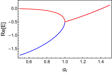
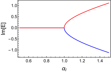
Figure 1: ${\cal PT}$ symmetry breaking for the ${\cal PT}$ symmetric delta function model. The two bound state eigenvalues are calculated using eq (20) with $\alpha_{R}=-1$ and $\beta=1$. The upper plot shows the real parts of the two eigenvalues and the lower plot shows the imaginary parts. The eigenvalues are plotted as a function of the parameter $\alpha_{I}$. The eigenvalues are found to undergo a characteristic complementary pitchfork bifurcation. Below the critical value $\alpha_{I}=1$ the eigenvalues are real and above they are a complex conjugate pair. The real parts of the eigenvalues degenerate at the critical value forming one pitchfork while the imaginary parts become non-zero forming the second complementary pitchfork.

In summary $|\alpha_{I}|>1$ and $-\alpha_{R}/\beta>0$ corresponds to the case of spontaneously broken ${\cal PT}$ symmetry. In this phase there are two bound states with complex conjugate energies. Otherwise ${\cal PT}$ symmetry is unbroken and there can be zero, one or two bound states all with real energy. The behavior of the bound state energies across the ${\cal PT}$ symmetry breaking transition exhibits a characteristic complementary pitchfork form illustrated in fig 1.

II.2.3 Scattering states

We now turn to the scattering of waves by a ${\cal PT}$ symmetric contact interaction. In ${\cal PT}$ quantum mechanics the $S$-matrix is no longer unitary and hence its eigenvalues are not required to be unimodular. When the eigenvalues are nonetheless unimodular ${\cal PT}$ symmetry is said to be intact; when they cease to unimodular ${\cal PT}$ is said to be spontaneously broken.

In order to determine the eigenvalues of the $S$-matrix we consider scattering states of the form

$$\psi = Ae^{ikx}+\lambda Be^{-ikx}\hskip 5.69054pt{\rm for}\hskip 5.69054ptx<0,$$ (22)

$$= \lambda Ae^{ikx}+Be^{-ikx}\hskip 5.69054pt{\rm for}\hskip 5.69054ptx>0.$$

Here the amplitudes of the incoming waves from the left and right, denoted $A$ and $B$ respectively, are amplified by the eigenvalue $\lambda$ in the corresponding outgoing waves. Making use of the boundary condition eq (2) yields two conditions connecting the ratio $A/B$ and $\lambda$. Imposing consistency between these expressions reveals that the eigenvalues of the $S$-matrix are the roots of the quadratic equation

$$\Delta\lambda^{2}+4ik\cos\theta\lambda-\Delta^{\ast}=0$$ (23)

where

$$\Delta=\gamma-\beta k^{2}-ik(\alpha+\delta).$$ (24)

In obtaining eq (23) we have assumed that $\beta,\gamma$ and $(\alpha+\delta)$ are real and that $\alpha\delta-\beta\gamma=1$. Hence our analysis to this point applies both to the hermitian and the ${\cal PT}$ symmetric contact interaction models.

It is evident from eq (23) that if $\lambda$ is an eigenvalue of the $S$-matrix then so is $1/\lambda^{\ast}$. It is also clear that the product of the magnitudes of the two eigenvalues must be 1. This also follows more generally because the $S$ matrix satisfies $S^{\dagger}S={\cal I}$ and $S^{\ast}S={\cal I}$ for the hermitian and ${\cal PT}$ symmetric cases respectively. (Here ${\cal I}$ denotes the $2\times 2$ identity matrix.)

By writing down the explicit solution to eq (23) it can be seen that if $|\Delta|>2k|\cos\theta|$ the eigenvalues are unimodular. On the other hand if $|\Delta|<2k|\cos\theta|$ the $S$-matrix eigenvalues no longer lie on the unit circle in the complex plane. One has a magnitude bigger than unity; the other, smaller, in order to ensure that the product of the magnitudes is still unity. Physically one eigenmode of the $S$-matrix is amplified upon scattering from the contact interaction; the other is attenuated.

Making use of eq (24) and exploiting $\alpha\delta-\beta\gamma=1$ yields the useful formula

$$|\Delta|^{2}-4k^{2}\cos^{2}\theta=(\gamma+\beta k^{2})^{2}+(\alpha-\delta)^{2}k^{2}+4k^{2}\sin^{2}\theta.$$ (25)

From eq (25) it is evident that in the hermitian case $\alpha=\delta$ and the right hand side is positive; hence $|\Delta|>2k|\cos\theta|$ always. In other words in the hermitian case we see by explicit calculation that the eigenvalues of the $S$ matrix must be unimodular as expected on general grounds also. However for the ${\cal PT}$ symmetric case $(\alpha-\delta)^{2}=-4\alpha_{I}^{2}$ and hence the middle term on the right hand side of eq (25) is negative. If it is sufficiently negative the eigenvalues of the $S$ matrix no longer have to lie on the unit circle and ${\cal PT}$ symmetry is said to be broken. Eq (25) reveals that there will always be a range of $k$ for which ${\cal PT}$ symmetry is broken so long as $\alpha_{I}^{2}>\sin^{2}\theta$ and $\alpha_{R}^{2}<\cos^{2}\theta$.

It is also interesting to examine the scattering amplitudes for the ${\cal PT}$ symmetric contact interaction; for simplicity we only consider the case $b\neq 0$ and $\theta=0$. If we consider a wave incoming from the left as in eq (15), then the scattering amplitude $t$ is still given by eq (16) but with $\kappa_{\pm}$ now given by eq (20). As for the hermitian case we see that the scattering amplitude has poles in the upper half $k$-plane that are determined by the bound states if any. Furthermore in case the bound state energies are a complex conjugate pair the scattering amplitude has a Lorentzian resonance whose location is determined by ${\rm Im}\;\kappa_{\pm}$ and width by ${\rm Re}\;\kappa_{\pm}$. This resonance has no counterpart in conventional hermitian quantum mechanics. The effect of a non-zero $\theta$ on the scattering amplitude is relatively innocuous; the amplitude is multiplied by $\exp(\pm i\theta)$ depending on whether the incident wave comes from $x\rightarrow\mp\infty$.

III Krönig-Penney Model

The Krönig-Penney model in one dimension is the simplest model of a crystal, originally introduced to provide a simple illustration of energy bands and band gaps in the early days of solid state physics. The model describes a particle that interacts with a periodic comb of delta functions that are separated by a distance $\ell$. Here we consider two generalizations of the textbook model wherein the ordinary delta function is replaced by either the generalized hermitian or the ${\cal PT}$ symmetric contact interactions introduced here. In the textbook case an isolated attractive delta function would have a single bound state. For a well separated array of delta function potentials this bound state fans out into a narrow band characterized by the energy dispersion $E(k)$ where $E$ is the energy of the Bloch state and $k$ its crystal momentum which lies in the Brillouin zone $-\pi/\ell<k<\pi/\ell$.

In the models considered here there can be two bound states in the isolated limit that fan into a pair of narrow bands when the contact potentials are well separated. We find that in the hermitian case the gap between the bands can close when the parameters are tuned suitably. The energy dispersion near the intersection of the two bands is approximately that of a massless Dirac particle. In the ${\cal PT}$ symmetric case we find that as the parameters are tuned the bands undergo a ${\cal PT}$ symmetry breaking transition. More precisely recall that for an isolated contact interaction the ${\cal PT}$ transition takes place for $|\alpha_{I}|=1$. For the corresponding Kronig-Penney model we find that for $|\alpha_{I}|<\alpha_{c1}<1$ the band energies $E_{\pm}(k)$ are entirely real; for $1<\alpha_{c2}<|\alpha_{I}|$ the band energies become complex conjugate; and for an intermediate range $\alpha_{c1}<|\alpha_{I}|<\alpha_{2}$ the band energies are real for a small range of $k$ and complex conjugate elsewhere in the Brillouin zone.

III.1 Bloch analysis

For a periodic potential in one dimension with a period $\ell$ the eigenfunctions must have the Bloch form

$$\psi_{nk}(x)=\Pi_{nk}(x)\exp(ikx)$$ (26)

Here $n$ is an index that labels the bands and $k$ is the crystal momentum which lies in the Brillouin zone $-\pi/\ell<k<\pi/\ell$. The form factor $\Pi_{nk}$ is a periodic function of $x$ with period $\ell$. Hence the Bloch wave-function obeys the quasi-periodic condition

$$\psi_{nk}(x+\ell)=\psi_{nk}(x)\exp(ik\ell)$$ (27)

In the Krönig-Penney model considered here we assume that the particle experiences a contact interaction at the points $x=\nu\ell$ where $\nu$ is an integer. This includes the origin which corresponds to $\nu=0$. Hence $\psi_{nk}$ must obey the boundary condition eq (2) at the origin. Since we are interested in bound state bands with negative energy we take the Bloch wave-function to have the form

$$\psi_{nk} = A\exp(\kappa x)+B\exp(-\kappa x)\hskip 8.53581pt{\rm for}\hskip 5.69054pt-\frac{\ell}{2}<x<0,$$

$$= C\exp(\kappa x)+D\exp(-\kappa x)\hskip 8.53581pt{\rm for}\hskip 5.69054pt0<x<\frac{\ell}{2}.$$

The energy of this state is $E=-\hbar^{2}\kappa^{2}/2$.

Imposing the quasi-periodicity condition (27) and the boundary condition (2) leads to the quantization condition

$$\kappa^{2}\beta+\kappa(\alpha+\delta)+\gamma = 4\kappa\cos(k\ell-\theta)e^{-\kappa\ell}$$

$$+ [\kappa^{2}\beta-\kappa(\alpha+\delta)+\gamma]e^{-2\kappa\ell}.$$

Our task now is to solve the transcendental equation (LABEL:eq:quantization) for $\kappa$. By determining the dependence of $\kappa$ on $k$ we can determine the energy dispersion $E(k)$. In the limit $\ell\rightarrow\infty$ the right hand side of eq (LABEL:eq:quantization) vanishes and the allowed $\kappa$ values are the same as for an isolated contact interaction as expected. The analysis for finite $\ell$ is undertaken separately below for the hermitian and ${\cal PT}$ symmetric cases. In both cases for simplicity we will take $\theta=0$ since the only effect of non-zero $\theta$ is to shift the bands in $k$-space.

III.2 ${\cal PT}$ symmetric bands

Recall that for the isolated ${\cal PT}$ symmetric contact interaction the allowed $\kappa$ values are given by eq (20). Since we are interested in the ${\cal PT}$ symmetry breaking transition we consider values of $|\alpha_{I}|$ near to the threshold value of unity. For brevity we write $\kappa_{\pm}=\overline{\kappa}\pm i\epsilon$ for $|\alpha_{I}|>1$ and $\kappa_{\pm}=\overline{\kappa}\pm\epsilon$ for $|\alpha_{I}|<1$ respectively. We assume that $\ell$ is sufficiently large that the bands will be narrow and hence posit that $\kappa=\overline{\kappa}+\Delta$ where $\Delta$ is small. To enforce that the bands are narrow we assume $\exp(-\kappa\ell)\ll 1$ and we also assume that $\Delta\ell\ll 1$. The condition $\exp(-\kappa\ell)\ll 1$ allows us to neglect the second term on the right hand side of the quantization condition and the condition that $\Delta\ell\ll 1$ allows us to approximate $\exp(-\kappa\ell)\approx\exp(-\overline{\kappa}\ell)$. Making these approximations yields

$$\Delta_{\pm}(k)=\pm W\sqrt{\varepsilon^{2}+\cos k\ell}$$ (30)

for $|\alpha_{I}|<1$ and

$$\Delta_{\pm}(k)=\pm W\sqrt{\cos k\ell-\varepsilon^{2}}$$ (31)

for $|\alpha_{I}|>1$. Here for simplicity we have defined

$$W=\left[\frac{4\overline{\kappa}}{\beta}\exp(-\overline{\kappa}\ell)\right]^{1/2}$$ (32)

and $\varepsilon$ is a rescaled version of $\epsilon$ given by $\epsilon=W\varepsilon$.

In summary the energy bands near the ${\cal PT}$ transition in the narrow band limit are given by the simple expression

$$E_{\pm}(k)=-\frac{1}{2}\overline{\kappa}^{2}-\overline{\kappa}\Delta_{\pm}(k)$$ (33)

where $\Delta_{\pm}(k)$ is given by eq (30) and (31) for the cases $|\alpha_{I}|<1$ and $|\alpha_{I}|>1$ respectively. $W$ is a measure of the bandwidth and $\varepsilon$ measures the distance of $|\alpha_{I}|$ from the transition value of unity. It is evident from these expressions that there are four regimes. (i) For the ${\cal PT}$ symmetric regime $|\alpha_{I}|<1$ and $\varepsilon>1$ and the bands are pure real. (ii) For the broken ${\cal PT}$ symmetry regime $|\alpha_{I}|>1$ and $\varepsilon>1$ the two bands are a complex conjugate pair. (iii) The range $|\alpha_{I}|<1$ and $\varepsilon<1$ corresponds to the onset of the ${\cal PT}$ transition. In this regime the bands are real for small $k$ and complex conjugate elsewhere in the Brillouin zone. (iv) The range $|\alpha_{I}|>1$ and $\varepsilon<1$ corresponds to the range over which the ${\cal PT}$ transition is completed. Over this range too the bands are partially real at small $k$ and complex conjugate elsewhere in the Brillouin zone. These behaviors are shown in fig 2.

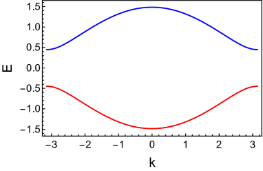
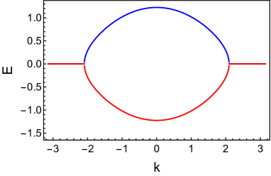
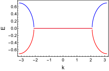
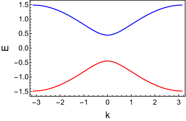
Figure 2: The energy bands of the ${\cal PT}$ symmetric Krönig-Penney model. The plot on top left shows the energy plotted as a function of wave-vector for the case of unbroken ${\cal PT}$ symmetry. This is the case (i) in the main text. The energy bands in this case are entirely real and have an approximate particle-hole symmetry. The plot on bottom right by contrast corresponds to case (iv) where the ${\cal PT}$ symmetry breaking transition is complete. The energy bands are a complex conjugate pair. The plot only shows the dispersion of the imaginary parts of the energy because the real part of the energies is found to be constant. The symmetry between the bands in this case is required by ${\cal PT}$ symmetry. The plots on top right and bottom left correspond to the onset of the ${\cal PT}$ transition. This is case (iii) in the text. The plot on top right shows the real part of the energy and the plot on the lower right shows the imaginary part. The bands have been offset so as to be centered about zero energy and the parameter $W=1$ and $\ell=1$ throughout whereas $\varepsilon^{2}=1.2$ (top left and bottom right) or $\varepsilon^{2}=0.5$ (top right and bottom left).

III.3 Hermitian bands

We now analyze the quantization condition eq (LABEL:eq:quantization) for the hermitian case. We focus on the case that for an isolated contact interaction there are two bound states. It is more convenient to work with the parameters $\kappa_{1},\kappa_{2}$ and $\beta$ that were introduced at the end of section II.2.1 to describe the contact interaction. In terms of these parameters the exact quantization condition (LABEL:eq:quantization) may be rewritten

$$(\kappa-\kappa_{1})(\kappa-\kappa_{2})=\frac{4\kappa}{\beta}\cos k\ell e^{-\kappa\ell}+(\kappa+\kappa_{1})(\kappa+\kappa_{2})e^{-2\kappa\ell}.$$ (34)

First for simplicity we assume that the two bound states are well separated in comparison to the width of the bands that they form. Now in order to analyze the band associated with the first isolated bound state we write $\kappa=\kappa_{1}+\Delta$ where $\Delta$ is assumed to be small. More precisely we assume that $\Delta\ell\ll 1$ and also that $\exp(-\kappa_{1}\ell)\ll 1$. The latter assumption allows us to ignore the second term on the right hand side of eq (34) and we obtain

$$\Delta=\frac{4\kappa_{1}}{\beta(\kappa_{1}-\kappa_{2})}e^{-\kappa_{1}\ell}\cos k\ell.$$ (35)

Recalling that the energy is given by $E=-\kappa^{2}/2$ we find that the first band has the energy dispersion

$$E_{1}(k)=-\frac{\kappa_{1}^{2}}{2}-\frac{4\kappa_{1}^{2}}{\beta(\kappa_{1}-\kappa_{2})}e^{-\kappa_{1}\ell}\cos k\ell$$ (36)

Similarly the second band is given by

$$E_{2}(k)=-\frac{\kappa_{2}^{2}}{2}+\frac{4\kappa_{2}^{2}}{\beta(\kappa_{1}-\kappa_{2})}e^{-\kappa_{2}\ell}\cos k\ell$$ (37)

More interesting behavior results when $\kappa_{1}\approx\kappa_{2}$. In this regime as the parameters of the generalized delta function potential are tuned appropriately the bands intersect at an isolated point in $k$-space before moving apart again. At the intersection the bands form a Dirac cone. To demonstrate this behavior we write $\kappa_{1}=\overline{\kappa}+\epsilon$ and $\kappa_{2}=\overline{\kappa}-\epsilon$ where $\epsilon$ is positive and assumed to be small in a sense to be made precise. As before we write $\kappa=\overline{\kappa}+\Delta$ where $\Delta$ is also assumed to be small. For simplicity we assume that the delta potentials are well separated, $\exp(-\overline{\kappa}\ell)\ll 1$, but that $\Delta$ is sufficiently small that $\Delta\ell\ll 1$. Due to the constraint $(\kappa_{1}-\kappa_{2})|\beta|=2\epsilon|\beta|\geq 2$, a small value of $\epsilon$ implies a large value of $\beta$; hence we can no longer neglect the second term on the right hand side of eq (34) in comparison to the first. In fact the two terms are of the same order if we take

$$\epsilon=2\overline{\kappa}e^{-\overline{\kappa}\ell}\varepsilon$$ (38)

where $\varepsilon$ is of order unity. We also write $1/\beta=f\epsilon$ with $-1<f<1$ (in order to respect the constraint $|\beta|\epsilon>1$). Making these assumptions and using eq (34) we obtain

$$\Delta=\pm 2\overline{\kappa}e^{-\overline{\kappa}\ell}\left(1+\varepsilon^{2}+2\varepsilon f\cos k\ell\right)^{1/2}.$$ (39)

This corresponds to the energy bands

$$E_{\pm}(k)=-\frac{\overline{\kappa}^{2}}{2}\mp 2\overline{\kappa}^{2}e^{-\overline{\kappa}\ell}\left[1+\varepsilon^{2}+2\varepsilon f\cos k\ell\right]^{1/2}.$$ (40)

From eq (40) we see that for $\varepsilon=1$ and $f=-1$ or $f=+1$ the bands touch at $k=0$ or $k=\pi$ respectively. For $k$ near the intersection the energy dispersion is approximately linear and the bands form a massless Dirac cone. In terms of the original parameters $\varepsilon=1$ and $f=\pm 1$ translates to $(\kappa_{1}-\kappa_{2})|\beta|=2$ where the sign of $\beta$ is the same as that of $f$. Put another way there are two gapped phases corresponding to $\beta>2/(\kappa_{1}-\kappa_{2})$ and $\beta<-2/(\kappa_{1}-\kappa_{2})$ respectively.

IV Conclusion

The delta function potential is a simple model of zero range contact interaction in one dimension. In this paper we have introduced generalizations of the delta function for conventional hermitian quantum mechanics and ${\cal PT}$ quantum mechanics in one dimension. We find that the corresponding generalizations of the Krönig-Penney model exhibit interesting behavior in both hermitian and ${\cal PT}$ quantum mechanics. In ${\cal PT}$ quantum mechanics we find bands that undergo ${\cal PT}$ symmetry breaking, providing a particularly simple example of this phenomenon. In hermitian quantum mechanics we find that the gap between the two bound state bands closes when the parameters of the interaction are appropriately tuned yielding a conical intersection between the bands at a single point in the Brillouin zone. Near the intersection the dispersion relation is that of a massless Dirac fermion. Whether the gapped phase on either side of gap closure is a topological insulator is an intriguing question we leave open for future work.

Another interesting application of our generalized contact interaction may be to many body physics in one dimension. There are only a handful of exactly soluble non-trivial models of quantum many body systems. In a seminal paper Lieb and Liniger showed that a one dimensional gas of bosons interacting via a delta function contact interaction was soluble via Bethe ansatz lieb ; mattis . There has been a resurgence of interest in this class of integrable models due to their experimental realization in cold atoms coldscience ; coldnature ; coldatoms A natural generalization of the Lieb-Liniger model suggested by this paper is to replace the delta function interaction with the generalized form of contact interaction studied here. This model also should be soluble via Bethe ansatz and may be realizable with cold atoms.

Acknowledgement. Kristin McKee was supported by SURES, a summer undergraduate research program of Case Western Reserve University.

References

- (1) In this context we use “hermitian” synonymously with the more precise term “self-adjoint”; see section II.1.
- (2) C.M. Bender and S. Boettcher, “Real spectra in non-Hermitian Hamiltonians having symmetry”, Phys. Rev. Lett. 80, 5243 (1998).
- (3) C.M. Bender, “Making sense of non-Hermitian Hamiltonians”, Reports on Progress in Physics 70, 947 (2007).
- (4) R. El-Ganainy et al., “Non-Hermitian physics and symmetry”, Nature Physics 14, 11 (2018).
- (5) L. Feng, R. El-Ganainy and L. Ge, “Non-hermitian photonics based on parity-time symmetry”, Nature Photonics 11, 752 (2017).
- (6) R. Jackiw, “Delta function potentials in two and three dimensional quantum mechanics”, in M.A.B. Bèg Memorial Volume, A. Ali and P. Hoodbhoy (eds) (World Scientific Singapore 1991).
- (7) Y.D. Chong, L. Ge and A.D. Stone, “-symmetry breaking and laser-absorber modes in optical scattering systems”, Phys. Rev. Lett. 106, 093902 (2011).
- (8) M.Z. Hasan and C.L. Kane, “Topological insulators”, Rev. Mod. Phys. 82, 3045 (2010).
- (9) J.H. Davies, The Physics of Low-dimensional Semiconductors (Cambridge University Press, Cambridge, 1997).
- (10) D. Krejcirik, H. Bila and M. Znojil, “Closed formula for the metric in the Hilbert space of a symmetric model”, J. Phys. A: Math. Gen. 39, 10143 (2006).
- (11) D. Krejcirik, “Calculation of the metric in the Hilbert space of a symmetric model via the spectral theorem”, J. Phys. A: Math. Theor. 41, 244012 (2008).
- (12) D. Krejcirik, P. Siegl, “ symmetric models in curved manifolds”, J. Phys. A: Math. Theor. 43, 485204 (2010).
- (13) H. Hernandez-Coronado, D. Krejcirik and P. Siegel, “Perfect transmission scattering as a symmetric spectral problem”, Phys. Lett. A 375, 2149 (2011).
- (14) D. Krejcirik, P. Siegel and J. Zelezny, “On the similarity of Sturm-Liouville operators with non-Hermitian boundary conditions to self-adjoint and normal operators”, Complex Anal. Oper. Theory 8, 255 (2014).
- (15) A. Dasarthy, J.P. Isaacson, K. Jones-Smith, J. Tabachnik and H. Mathur, “The particle in a box in PT quantum mechanics and an electromagnetic analog”, Phys. Rev. A87, 062111 (2013).
- (16) C.M. Bender, G.V. Dunne and P.N. Meisinger, “Complex periodic potentials with real band spectra”, Phys. Lett. A 252 272 (1999).
- (17) H. F. Jones, “The energy spectrum of complex periodic potentials of the Krönig-Penney type”, Phys. Lett. A 262, 242 (1999).
- (18) Z. Ahmed, “Energy band structure due to a complex periodic invariant potential”, Phys. Lett. A 286, 231 (2001).
- (19) K.G. Makris, R. El-Ganainy, D.N. Christodoulides, “Beam dynamics in symmetric optical lattices”, Phys. Rev. Lett. 100, 103904 (2008).
- (20) A.D. Shapere, F. Wilczek and Zhaoxi Xiong, “Models of topology change”, arXiv:1210.3545.
- (21) M. Stone and P. M. Goldbart, Mathematics for physics: a guided tour for graduate students (Cambridge University Press, Cambridge, 2009).
- (22) Naively one might suppose that it is possible to eliminate the phase by making the following gauge transformation: for and for . However even for an open one dimensional system physics is invariant only under small gauge transformations where for . Indeed we will see below that although the bound states are independent of the scattering matrix does depend on in a non-trivial way. This is a particularly simple example of the subtle distinction between large and small gauge transformations in quantum mechanics.
- (23) E.H. Lieb and W. Liniger, “Exact Analysis of an Interacting Bose Gas. I. The General Solution and the Ground State”, Phys. Rev. 130, 1605 (1963).
- (24) D. Mattis, The Many Body Problem. An encyclopedia of exactly solved models in one dimension (World Scientific, Singapore, 1993).
- (25) T. Kinoshita, T. Wenger and D.S. Weiss, “Observation of a one-dimensional Tonks-Girardeau gas”, Science 305, 1125 (2004).
- (26) B. Paredes et al., “Tonks-Girardeau gas of ultracold atoms in an optical lattice”, Nature 429, 277 (2004).
- (27) I. Bloch, J. Dalibard and W. Zwerger, “Many-body physics with ultracold gases”, Rev. Mod. Phys. 80, 885 (2008).