Simulations of intermittent two-phase flows in pipes using smoothed particle hydrodynamics

Abstract

Slug flows are a typical intermittent two-phase flow pattern that can occur in submarine pipelines connecting the wells to the production facility and that is known to cause undesired consequences. In this context, computational fluid dynamics appears to be the tool of choice to understand their formation. However, few direct numerical simulations of slug flows are available in the literature, especially using meshless methods which are known to be capable of handling complex problems involving interfaces.

In this work, a 2D study of the instability processes leading to the formation of intermittent flows in pipes is conducted using an existing multiphase smoothed particle hydrodynamics formulation associated with inlet and outlet boundary conditions. This paper aims to demonstrate the applicability of smoothed particle hydrodynamics to a given set of close-to-industry cases.

First, we check the ability of our implementation to reproduce flow regimes predicted by Taitel and Duckler’s flow map. Then, we focus on the transition processes from one flow pattern to the other. Finally, we present the results obtained for more realistic cases with high density and viscosity ratios.

1 Introduction

Two-phase flows problems involving non-miscible fluids with a deformable interface are encountered in numerous industrial and scientific applications [25]. One of the main examples is the transportation of oil and gas (or oil and water) through pipelines in the petroleum industry. However, gas-liquid flows are also present in chemical and heat transfer systems such as evaporators, boilers, condensers, distillation processes, air-conditioning or refrigerators and liquid-liquid flows are fundamental in solvent extraction equipments such as pulsed columns. Furthermore, all these two phase flows can also be found in natural environments and are studied in meteorology for instance.

The main focus of this work is the emergence of intermittent flow patterns (also known as slug or plug flow [13]) which only occurs in gas-liquid or liquid-liquid flows. In particular, in pipeline networks, these patterns are highly undesirable [52]. Those slug patterns, that can measure up to tens of meters, are known to damage facilities (separators flooding, compressors starving, water hammer phenomenon) and to reduce flow efficiency. Besides, intermittent flows are also commonly found in microfluidic applications in the chemical industry where they can improve reactions performances [65, 73].

The mechanisms of generation of slug flows are well known. On one hand, in the case of horizontal pipes, hydrodynamic slugs are induced by the Kelvin-Helmholtz instability. Under certain velocity and geometry conditions, liquid waves can grow in the flow causing a local increase of the gas velocity and a local decrease of the pressure. Consequently, a suction force starts to move the interface higher until reaching the top of the pipe and forming a slug. A common way to avoid the appearance of hydrodynamic slugs is to use flow regime maps to operate with flow conditions that are unlikely to generate them.

On the other hand, intermittent flows can be caused by the combined effects of gravity and terrain geometry on which the pipe lies [50]. The path of the pipe can have low spots, like elbows, in which the liquid is trapped. It accumulates until reaching the top of the pipe and it is then carried away by the flow forming a slug. Alternatively, severe slugging can occur in risers. In a nutshell, a liquid slug begins to form at the riser base blocking the incoming gas. Moved by the increasing gas pressure, the liquid fills up the riser forming a slug that flood the separator at the end of the riser. Additionally, slugging can be generated by a flow rate change or by pigging.

The main question when studying slugging is to know whether or not it will occur and eventually to find the criterion that triggers its formation [77]. If it does, the quantities of interest are the size of slugs and their transit time and frequency.

The understanding of the formation of intermittent flow patterns has been a lively research area for years. In this context, Computational Fluid Dynamics (CFD) softwares [38, 48] emerged as a useful tool to predict the appearance of a slug flow regime in the oil and gas industry.

Early simulations were based on steady state models [60, 66] and transient models [51] and were able to simulate slugging in gravity-dominated flows. In the oil and gas industry, two commercial softwares are competing for slugging simulation : OLGA developed by SPT group [6] and LedaFlow, proposed by Kongsberg [29]. A detailed comparison of both softwares that can be found in [5] concludes that although performing equally well on simple cases, they have trouble to simulate complex cases with a dominant gas phase.

From an academic perspective, different methods have been used for slug flow modeling such as volume-of-fluid [59, 1], level-set [18, 36], lattice boltzmann [75] or phase field [24, 72] but they are mostly focused on microfluidic problems.

The method known as Smoothed Particle Hydrodynamics (SPH) is becoming more and more popular throughout the years. Indeed, thanks to its meshless nature, SPH emerged as an interesting tool to model multiphase flows and many authors have applied it to solve complex multiphase problems [70]. Nevertheless, SPH or more generally meshless simulations of slug flows are not common in the literature despite the inherent benefits of being meshfree for tackling interfaces problems. To the best of our knowledge, the only previous SPH study on the topic is available in [39] and is focused on the transition from bubbly flow to slug flow using periodic boundary conditions and a gravity-based driving force.

Our goal with this work is to contribute to the ongoing effort to show that SPH can be applied to industrial cases. To this end, we used recent multiphase SPH features available in the literature to a set of close-to-industry test cases.

In this paper, we first detail the multiphase SPH formulation introduced in [26] including the surface tension model presented in [32] and with particular emphasis on how to handle inlet/outlet boundary conditions in a multiphase context in sections 2 to 4. Then, in sections 5.1 and 5.2, we verify the ability of our SPH model to recover different flow regimes predicted by Taitel and Dukler’s flow map [61] and we study the transition processes between two flow patterns. Finally, in section 5.3, we present two more realistic cases involving high density and viscosity ratios.

A collection of quantitative validation cases of our implementation for both single phase and multiphase problems is presented in A.

2 Governing Equations

In this section, the main governing equations of the considered problem are recalled in details.

2.1 Single phase balance equations

The governing equations of the problem for a single fluid phase consist of mass and momentum conservation equations in a Lagrangian system, and are given as

$$\frac{D\rho}{Dt} =-\rho\nabla\cdot\bm{u},$$ (2.1)

$$\rho\frac{D\bm{u}}{Dt} =-\nabla p+\nabla\cdot\bm{\tau}+\rho\bm{g},$$ (2.2)

with $\bm{u}$ fluid velocity, $\rho$ fluid density, $\bm{\tau}$ viscous stress tensor, $p$ fluid pressure, $\mu$ fluid dynamic viscosity, $\bm{g}$ gravity and $D/Dt$ denotes the material derivative following the motion. Note that, in the case of an incompressible fluid with a constant viscosity, the viscous term reduces to $\nabla\cdot\bm{\tau}=\mu\nabla^{2}\bm{u}$ with $\mu$ the fluid viscosity.

A constitutive relation for the evaluation of $p$ has to be added to the governing equations (2.1)-(2.2) to close the system. In this paper, the Tait’s equation of state has been used. It reads

$$p=\frac{c^{2}\rho^{0}}{\gamma}\left[\left(\frac{\rho}{\rho_{0}}\right)^{\gamma}-1\right]+p_{0},$$ (2.3)

with $c$ fluid speed of sound (here constant), $\gamma$ fluid adiabatic index, $\rho_{0}$ fluid initial density and $p_{0}$ background pressure.

This approach is known as the Weakly Compressible SPH formulation (WCSPH). It is not a truly incompressible approach since the density is allowed to vary because of the Lagrangian nature of the algorithm. This artificial compressibility has to be as weak as possible and is controlled by the speed of sound $c$. Universal guidelines to set a good value for $c$ and $p_{0}$ are not available. It is common to set a value and adjust it on a case by case basis. In this paper, given a reference length $L_{\text{ref}}$ and a reference speed $U_{\text{ref}}$, the following formulas, taken from [45], were used

$$\left\{\begin{array}[]{l l}c_{\alpha}&=\max\left(\frac{U_{\text{ref}}}{\sqrt{\Delta\rho}},\sqrt{\frac{\lvert\bm{g}\rvert L_{\text{ref}}}{\Delta\rho}},\sqrt{\frac{\sigma^{\alpha\beta}}{\rho_{0\alpha}L_{\text{ref}}}},\sqrt{\frac{\mu_{\alpha}U_{\text{ref}}}{\rho_{0\alpha}L_{\text{ref}}\Delta\rho}}\right),\quad\forall\alpha\in\{1,\ldots,N_{\text{phases}}\},\\ p_{0}&=\max_{\alpha\in\{1,\ldots,N_{\text{phases}}\}}\frac{c^{2}_{\alpha}\rho_{0\alpha}}{\gamma_{\alpha}},\end{array}\right.$$ (2.4)

with $\Delta\rho=0.01$ to enforce (not strictly) a maximum variation of $1\%$ of the density field and $\sigma^{\alpha\beta}$ the surface tension coefficient between phase $\alpha$ and $\beta$. $N_{\text{phases}}$ is the number of different phases. Some authors recommend to use $p_{0}=0.1\max_{\alpha\in\{1,\ldots,N_{\text{phases}}\}}\frac{c^{2}_{\alpha}\rho_{0\alpha}}{\gamma_{\alpha}}$ but we were not able to obtain stable simulations with such low values. The background pressure helps stabilizing the simulations but can lead to pressure noises if set too high [68]. In this work, we have not done an exhaustive sensitivity study and used the expression given in (2.4). It might be possible to adjust more carefully the background pressure for each case to attenuate pressure oscillations.

2.2 Surface tension

In the case of a multiphase flow system, each phase is governed by the set of equations (2.1), (2.2) and (2.3). An interaction force has to be added to the momentum equation to model surface tension between fluids. The continuum surface stress method introduced by [32] has been used to that end. In this approach, the surface tension force per unit volume is expressed as the divergence of the capillary pressure tensor

$$\bm{F}^{st}=-\nabla\cdot\Pi,$$ (2.5)

with $\Pi$ the capillary pressure tensor defined by

$$\Pi=\sum_{\alpha,\beta\mid\alpha<\beta}\Pi^{\alpha\beta},$$ (2.6)

where $\alpha,\beta\in\{1,\ldots,N_{\text{phases}}\}$ and $\Pi^{\alpha\beta}$ is expressed as

$$\Pi^{\alpha\beta}=-\sigma^{\alpha\beta}\left(\bm{I}-\tilde{\bm{n}}^{\alpha\beta}\otimes\tilde{\bm{n}}^{\alpha\beta}\right)\delta^{\alpha\beta},$$ (2.7)

with $\tilde{\bm{n}}^{\alpha\beta}$ the unit normal vector from phase $\alpha$ to phase $\beta$, $\sigma^{\alpha\beta}$ the surface tension coefficient between phase $\alpha$ and phase $\beta$, $\delta^{\alpha\beta}$ a well-chosen surface delta function and $\bm{I}$ the identity matrix.

In the case of a three-phase system with a wetting phase $s$, a non wetting phase $n$ and a solid phase $s$ as described in Figure 1, the stress tensor reads $\Pi=\Pi^{ns}+\Pi^{ws}+\Pi^{nw}$.

There are at least two other approaches to represent surface tension in an SPH formulation. One is very similar to the one that was used in this paper and is based on curvature computation [8, 45] and the other one is based on pairwise forces [62].

The full set of governing equations including surface tension for an incompressible fluid is given as

$$\left\{\begin{array}[]{l l}\frac{D\rho}{Dt}&=-\rho\nabla\cdot\bm{u},\\ \frac{D\bm{u}}{Dt}&=-\frac{\nabla p}{\rho}+\nu\nabla^{2}\bm{u}+\frac{\bm{F}^{st}}{\rho}+\bm{g},\\ p&=\frac{c^{2}\rho_{0}}{\gamma}\left[\left(\frac{\rho}{\rho_{0}}\right)^{\gamma}-1\right]+p_{0},\end{array}\right.$$ (2.8)

with $\nu=\frac{\mu}{\rho}$ the kinematic viscosity.

Figure 1: A triple point contact line between a non wetting phase $\Omega_{n}$, a wetting phase $\Omega_{w}$ and a solid phase $\Omega_{s}$ with their associated unit normal vectors $\tilde{\bm{n}}_{ab}$ and boundary lines $\Gamma_{ab}$

3 SPH Formulation

In this section, we introduce the SPH formulation used throughout this paper.

3.1 Standard SPH Formulation

An SPH discretization consists of a set of points with fixed volume, which possess material properties and interact with all neighboring particles through a weighting function (or smoothing kernel) [21]. A particle’s support domain, $\Lambda$, is given by its smoothing length, $h$, which is the radius of the smoothing kernel. In all simulations presented in this paper, $h=2\Delta r$ where $\Delta r$ is the initial particle spacing. To obtain the value of a function at a given particle location, values of that function are found by taking a weighted (by the smoothing function) interpolation from all particles within the given particle’s support domain. Analytical differentiation of the smoothing kernel is used to find gradients of this function. Detailed concepts and descriptions of this method are given by Monaghan [41].

To begin, we define the following kernel estimation

$$\bm{A}(\bm{x})=\int_{\Omega}{\bm{A}(\bm{x}^{\prime})W(\bm{x-x^{\prime}},h)}\,d\bm{x}^{\prime},\leavevmode\nobreak\ \leavevmode\nobreak\ \leavevmode\nobreak\ \leavevmode\nobreak\ \leavevmode\nobreak\ \leavevmode\nobreak\ \leavevmode\nobreak\ \leavevmode\nobreak\ \forall\leavevmode\nobreak\ \bm{x}\in\Omega\subset\mathbb{R}^{d}\leavevmode\nobreak\ \leavevmode\nobreak\ \leavevmode\nobreak\ \leavevmode\nobreak\ \leavevmode\nobreak\ \leavevmode\nobreak\$$ (3.1)

where $\bm{A}$ is a vector function of the position vector $\bm{x}$, $\Omega$ is the integral space containing the point $\bm{x}$, and $W(\bm{x-x^{\prime}},h)$ is the smoothing kernel. The interpolated value of a function $\bm{A}$ at the position $\bm{x}_{a}$ of particle $a$ can be expressed using SPH smoothing as

$$\bm{A}(\bm{x}_{a})=\sum_{b\in\Lambda_{a}}\bm{A}_{b}\frac{m_{b}}{\rho_{b}}W(\bm{x}_{a}-\bm{x}_{b},h),$$ (3.2)

in which $\bm{A}_{b}=\bm{A}(\bm{x}_{b})$, $m_{b}$ and $\rho_{b}$ are the mass and the density of neighboring particle $b$. The set of particles $\Lambda_{a}=\{b\in\mathbb{N}\mid\lvert\bm{x}_{a}-\bm{x}_{b}\rvert\leq\kappa h\}$ contains neighbors of particle $a$ and lie within its defined support domain. The coefficient $\kappa$ depends on the choice of the kernel, it is equal to $2$ for the $5^{th}$ order $\mathcal{C}^{2}$ Wendland kernel function [71, 10]) used in this paper. In 2D, this kernel is expressed as follows

$$W(q,h)=\frac{7}{4\pi h^{2}}\left(1-\frac{q}{2}\right)^{4}\left(1+2q\right),$$ (3.3)

with $q=\frac{\lvert\bm{x}_{a}-\bm{x}_{b}\rvert}{h}$, $q\leq 2$.

Gradient and divergence operators of the function $\bm{A}$ at the position of particle $a$ are evaluated by differentiating the smoothing kernel $W$ in equation (3.2) as

$$\nabla\bm{A}(\bm{x}_{a}) =\sum_{b\in\Lambda_{a}}\bm{A}_{b}\frac{m_{b}}{\rho_{b}}\nabla_{a}W(\bm{x}_{a}-\bm{x}_{b},h),$$ (3.4)

$$\nabla\cdot\bm{A}(\bm{x}_{a}) =\sum_{b\in\Lambda_{a}}\bm{A}_{b}\frac{m_{b}}{\rho_{b}}\cdot\nabla_{a}W(\bm{x}_{a}-\bm{x}_{b},h).$$ (3.5)

In practice, Libersky et al. find that by exploiting the symmetric properties of the kernel, a more accurate formulation is found [35] as

$$\nabla\bm{A}(\bm{x}_{a}) =-\frac{1}{\rho_{a}}\sum_{b\in\Lambda_{a}}\bm{A}_{ab}m_{b}\nabla_{a}W_{ab},$$ (3.6)

$$\nabla\cdot\bm{A}(\bm{x}_{a}) =-\frac{1}{\rho_{a}}\sum_{b\in\Lambda_{a}}\bm{A}_{ab}m_{b}\cdot\nabla_{a}W_{ab}.$$ (3.7)

where, for the sake of clarity, $W(\bm{x}_{a}-\bm{x}_{b},h)$ and $\bm{A}_{a}-\bm{A}_{b}$ have been denoted $W_{ab}$ and $\bm{A}_{ab}$ respectively. These notations will be used in the rest of the paper.

3.2 Multiphase SPH Formulation

Since the introduction of the SPH method, several specific formulations designed for multiphase problems have been introduced. Among them, one can mention [9, 22, 64] and [76]. In this paper, the formalism introduced in [26] has been used. In this framework, the continuity equation (2.1) is not discretized directly. A common practice in SPH for flows that do not involve any free surface, the density is directly evaluated through a kernel summation. This approach gives an exact solution to the continuity equation. Traditionally in SPH, this kernel summation is $\rho_{a}=\sum_{b\in\Lambda_{a}}m_{b}W_{ab}$ but in the present framework, it is

$$\rho_{a}=m_{a}\sum_{b\in\Lambda_{a}}W_{ab}.$$ (3.8)

The difference is that the density evaluation for a given particle $a$ does not take into account the masses of neighboring particles which allows the treatment of density discontinuities.

Discretized gradient and divergence operators in this formalism are given by

$$\nabla\bm{A}(\bm{x}_{a})=\sum_{b\in\Lambda_{a}}\left(\frac{\bm{A}_{a}}{\Theta_{a}^{2}}+\frac{\bm{A}_{b}}{\Theta_{b}^{2}}\right)\Theta_{a}\nabla_{a}W_{ab},$$ (3.9)

$$\nabla\cdot\bm{A}(\bm{x}_{a})=\sum_{b\in\Lambda_{a}}\left(\frac{\bm{A}_{a}}{\Theta_{a}^{2}}+\frac{\bm{A}_{b}}{\Theta_{b}^{2}}\right)\Theta_{a}\nabla_{a}\cdot W_{ab},$$ (3.10)

where $\Theta_{a}=\frac{\rho_{a}}{m_{a}}$. It follows that the discretized pressure term $-\frac{\nabla p_{a}}{\rho_{a}}$ for a particle $a$ is given by

$$-\frac{\nabla p_{a}}{\rho_{a}}=-\frac{1}{m_{a}}\sum_{b\in\Lambda_{a}}\left(\frac{p_{a}}{\Theta_{a}^{2}}+\frac{p_{b}}{\Theta_{b}^{2}}\right)\nabla_{a}W_{ab},$$ (3.11)

where the pressures $p_{a}$ and $p_{b}$ are computed using the equation of state (2.3). The discretized viscous term $\nu_{a}\nabla^{2}\bm{u}_{a}$ for a particle $a$ is discretized using the inter-particle averaged shear stress [16] leading to

$$\nu_{a}\nabla^{2}\bm{u}_{a}=\frac{1}{m_{a}}\sum_{b\in\Lambda_{a}}\frac{2\mu_{a}\mu_{b}}{\mu_{a}+\mu_{b}}\left(\frac{1}{\Theta_{a}^{2}}+\frac{1}{\Theta_{b}^{2}}\right)\frac{\bm{x}_{ab}\cdot\nabla_{a}W_{ab}}{\lvert\bm{x}_{ab}\rvert^{2}+\eta^{2}}\bm{u}_{ab},$$ (3.12)

where $\eta=0.01h$ is a safety factor to avoid a division by zero. The discretized surface tension term $\frac{\bm{F}^{st}_{a}}{\rho_{a}}$ for a particle $a$ is given by

$$\frac{\bm{F}^{st}_{a}}{\rho_{a}}=-\frac{1}{m_{a}}\sum_{b\in\Lambda_{a}}\left(\frac{\Pi_{a}}{\Theta_{a}^{2}}+\frac{\Pi_{b}}{\Theta_{b}^{2}}\right)\nabla_{a}W_{ab},$$ (3.13)

where the stress tensors $\Pi_{a}$ and $\Pi_{b}$ are computed using equations (2.6)-(2.7).

Note that in SPH, the evaluation of normals is performed through the computation of the gradient of a color function $\chi$ defined for a given particle $a$ and a given phase $\alpha$ as

$$\chi^{\alpha}_{a}=\begin{cases}1\quad\text{if }a\in\text{phase }\alpha,\\ 0\quad\text{else}.\end{cases}$$ (3.14)

The normal vector $\bm{n}^{\alpha\beta}_{a}$ of particle $a$ belonging to phase $\alpha$ to the interface $\alpha\beta$ is then computed doing

$$\bm{n}^{\alpha\beta}_{a}=\nabla\chi^{\alpha\beta}_{a}=\sum_{b\in\Lambda_{a}}\left(\frac{\bm{\chi}^{\beta}_{a}}{\Theta_{a}^{2}}+\frac{\bm{\chi}^{\beta}_{b}}{\Theta_{b}^{2}}\right)\Theta_{a}\nabla_{a}W_{ab}.$$ (3.15)

The surface delta function $\delta^{\alpha\beta}_{a}$ is chosen to be equal to $\lvert\bm{n}^{\alpha\beta}_{a}\rvert$ and $\tilde{\bm{n}}^{\alpha\beta}=\bm{n}^{\alpha\beta}_{a}/\lvert\bm{n}^{\alpha\beta}_{a}\rvert$.

Moreover, due to its Lagrangian nature, the SPH particles are moved using simply

$$\frac{D\bm{x}_{a}}{Dt}=\bm{u}_{a}.$$ (3.16)

Ultimately, the full multiphase SPH formulation for a particle $a$ can be summarized as follows

$$\left\{\begin{array}[]{l l}\rho_{a}&=m_{a}\sum_{b\in\Lambda_{a}}W_{ab},\\ \frac{D\bm{u}}{Dt}&=-\frac{1}{m_{a}}\sum_{b\in\Lambda_{a}}\left(\frac{p_{a}\bm{I}+\Pi_{a}}{\Theta_{a}^{2}}+\frac{p_{b}{I}\bm{+}\Pi_{b}}{\Theta_{b}^{2}}\right)\nabla_{a}W_{ab}\\ &\quad+\frac{1}{m_{a}}\sum_{b\in\Lambda_{a}}\frac{2\mu_{a}\mu_{b}}{\mu_{a}+\mu_{b}}\left(\frac{1}{\Theta_{a}^{2}}+\frac{1}{\Theta_{b}^{2}}\right)\frac{\bm{x}_{ab}\cdot\nabla_{a}W_{ab}}{\lvert\bm{x}_{ab}\rvert^{2}+\eta^{2}}\bm{u}_{ab}\\ &\quad+\bm{g},\\ p_{a}&=\frac{c^{2}_{a}\rho_{0a}}{\gamma_{a}}\left[\left(\frac{\rho_{a}}{\rho_{0a}}\right)^{\gamma_{a}}-1\right]+p_{0},\\ \frac{D\bm{x}_{a}}{Dt}&=\bm{u}_{a}.\end{array}\right.$$ (3.17)

3.3 Corrective terms

In this work, three SPH correction procedures have been used. First, as suggested in [7], the kernel gradient are modified in order to restore consistency. For a given particle $a$, it reads

$$\widetilde{\nabla W}_{ab} =\bm{L}_{a}\nabla W_{ab},$$ (3.18)

where $\bm{L}_{a}=\left(\sum_{b\in\Lambda_{a}}\frac{m_{a}}{\rho_{a}}\nabla W_{ab}\otimes(\bm{x}_{b}-\bm{x}_{a})\right)^{-1}$. Note that the tilde notation will be dropped in the rest of paper although the kernel gradient correction will be always used.

Second, the shifting technique for multiphase flows introduced in [40] has also been used to maintain a good particles distribution. At the end of every timestep, all particles are shifted by a distance $\delta\bm{r}^{s}$ from their original position. This shifting distance of a particle $a$ is evaluated by doing

$$\delta\bm{r}^{s}_{a}=\left\{\begin{array}[]{l l}-D_{a}\nabla C_{a}\quad\text{if }a\in\text{light phase}\\ -D_{a}\left(\frac{\partial C_{a}}{\partial s}\bm{s}+\alpha_{n}\left(\frac{\partial C_{a}}{\partial n}\bm{n}-\beta_{n}\right)\right)\quad\text{if }a\in\text{heavy phase}\end{array}\right.$$ (3.19)

where $C_{a}=\sum_{b\in\Lambda_{a}}\frac{m_{a}}{\rho_{a}}W_{ab}$ is the particle concentration, $\nabla C_{a}=\sum_{b\in\Lambda_{a}}\frac{m_{a}}{\rho_{a}}(C_{b}-C_{a})\nabla W_{ab}$ is the particle concentration gradient, $D_{a}$ is the diffusion coefficient, $\bm{s}$ and $\bm{n}$ are respectively the tangent and normal vectors to the interface light/heavy phase (with $\bm{n}$ oriented towards the light phase), $\beta_{n}$ is a reference concentration gradient (taken equal to its initial value) and $\alpha_{n}$ is the normal diffusion parameter and is set equal to $0.1$. The diffusion coefficient $D_{a}$ is computed as follows

$$D_{a}=A_{s}\lvert\bm{u}_{a}\rvert\Delta t$$ (3.20)

where $A_{s}$ is a parameter set to $2$, $\bm{u}_{a}$ is the velocity of particle $a$, and $\Delta t$ is the timestep.

Third, as reported by several authors [9, 22, 55, 19], multiphase SPH can suffer from sub-kernel micro-mixing phenomena. Around the interface, within a distance corresponding ot the range of the kernel smoothing, particles have a tendency to mix. It is due to the fact that there is no mechanism ensuring phases immiscibility in the surface tension’s continuum surface stress model. As suggested by the previously mentioned authors, we introduce a small repulsive force between phases as follows

$$\bm{F}^{corr}_{a}=\varepsilon\sum_{b\in\Lambda_{a},b\notin\Omega_{a}}\left(\frac{1}{\Theta_{a}^{2}}+\frac{1}{\Theta_{b}^{2}}\right)\nabla_{a}W_{ab},$$ (3.21)

where $\varepsilon=\frac{L_{\text{ref}}}{h}$ for all simulations as suggested  in [56] where $L_{\text{ref}}$ is a reference length, typically the diameter for pipes. Note that the alternative formulation given by $\bm{F}^{corr}_{a}=\varepsilon\sum_{b\in\Lambda_{a},b\notin\Omega_{a}}\left(\frac{p_{a}}{\Theta_{a}^{2}}+\frac{p_{b}}{\Theta_{b}^{2}}\right)\nabla_{a}W_{ab}$ with $\varepsilon=0.1$ produces roughly the same force magnitude at the interface. The impact of this corrective force on the simulation of the same test cases studied in this paper can be found in [12].

3.4 Time Integration

As with other numerical methods, any time integration scheme could be used. For the SPH method, both the Velocity Verlet and Predictor-Corrector Leapfrog schemes have proven popular. For this work, the Predictor-Corrector Leapfrog scheme was adopted as it was shown in [63] to be more stable than the Velocity Verlet scheme in the presence of boundary conditions.

The algorithm is described hereafter. For every particle $a$,

1. Predictor Step

   $$\bm{u}^{n}=\left\{\begin{array}[]{l l}\bm{u}^{0}\quad\text{if }t=0\\ \bm{u}^{n-\frac{1}{2}}+\frac{\Delta t}{2}{\frac{D\bm{u}}{Dt}}^{n-1}\quad\text{if }t>0\end{array}\right.$$ (3.22)

2. Compute $\rho^{n}_{a}$ and $p^{n}_{a}$ using the corresponding expressions in equation (3.17).

3. Evaluate $\frac{D\bm{u}}{Dt}^{n}$ using the momentum equation in (3.17).

4. Corrector Step

   $$\bm{u}^{n+\frac{1}{2}}=\left\{\begin{array}[]{l l}\bm{u}^{n}+\frac{\Delta t}{2}{\frac{D\bm{u}}{Dt}}^{n}\quad\text{if }t=0\\ \bm{u}^{n-\frac{1}{2}}+\Delta t{\frac{D\bm{u}}{Dt}}^{n}\quad\text{if }t>0\end{array}\right.$$ (3.23)

   $$\bm{x}^{n+1}=\bm{x}^{n}+\Delta t\bm{u}^{n+\frac{1}{2}}$$ (3.24)

The time step $\Delta t$ has to respect the Courant-Friedrichs-Lewy (CFL) criteria to ensure a stable evolution of the system e.g.

$$\Delta t=\min\left(\Delta t_{\text{visc}},\Delta t_{\text{grav}},\Delta t_{\text{speed}},\Delta t_{\text{st}}\right),$$ (3.25)

where, following [45], we have

$$\left\{\begin{array}[]{l l}\Delta t_{\text{visc}}&=0.125\,\min_{\alpha\in\{1,\ldots,N_{\text{phases}}\}}\frac{h^{2}\rho^{0}_{\alpha}}{\mu_{\alpha}},\\ \Delta t_{\text{grav}}&=0.25\,\sqrt{\frac{h}{\lvert\bm{g}\rvert}},\\ \Delta t_{\text{speed}}&=0.25\,\min_{\alpha\in\{1,\ldots,N_{\text{phases}}\}}\frac{h}{c_{\alpha}},\\ \Delta t_{\text{st}}&=0.25\,\min_{\alpha,\beta\in\{1,\ldots,N_{\text{phases}}\}}\sqrt{\frac{h^{3}\rho^{0}_{\alpha}}{2\pi\sigma^{\alpha\beta}}}.\end{array}\right.$$ (3.26)

A recent article [68] investigated in detail what is the maximum admissible timestep in the WCSPH context.

4 Boundary Conditions

Figure 2: Schematic of a ghost particle $g$ (in black) and its associated support domain $\Lambda_{g}$ (hatched area) intersecting with the fluid domain $\Omega_{f}$ (gray particles) and the ghost domain $\Omega_{g}$ (white particles) separated by $\Gamma_{fg}$.

Because SPH is a collocation method, the treatment of boundary conditions is far from being trivial and is an active area of research within the community. The SPH European Research Interest Community (SPHERIC) even made this topic one of its Grand Challenges for the development of the SPH method (http://spheric-sph.org).

Originally, in order to impose wall Boundary Conditions (BC), repulsive forces based on the Lennard-Jones potential were used [43]. However, it was shown in [15] that it induces strong spurious behaviors near the boundaries. Today, most models are imposing wall BC through the use of ghost particles or mirror particles [44, 9, 47, 74]. Recently, a new approach using semi-analytical BC was introduced in [15, 34, 14] for both wall and inlet/outlet BC. However, this semi-analytical approach is significantly more complex and time consuming, we preferred to use a simpler approach in view of the simple test cases that we consider in this work.

In this work, we used several types of BC : no-slip wall (superscript $w$) and inlet/outlet (superscripts $in$ and $out$). For no-slip wall BC, the ghost particle method has been used along with the following prescribed values for the pressure $p^{w}$, density $\rho^{w}$ and velocity $\bm{v}^{w}$ for a given ghost particle $g$

$${p^{w}_{g}} =\frac{1}{V_{ga}}\sum_{a\in\Omega_{f}\cap\Lambda_{g}}p_{a}\frac{m_{a}}{\rho_{a}}W_{ga},$$ (4.1)

$${\rho^{w}_{g}} =\frac{1}{V_{ga}}\sum_{a\in\Omega_{f}\cap\Lambda_{g}}\rho_{a}\frac{m_{a}}{\rho_{a}}W_{ga},$$ (4.2)

$${\bm{v}^{w}_{g}} =\frac{-1}{V_{ga}}\sum_{a\in\Omega_{f}\cap\Lambda_{g}}\bm{v}_{a}\frac{m_{a}}{\rho_{a}}W_{ga},$$ (4.3)

with $V_{ga}=\sum_{a\in\Omega_{f}\cap\Lambda_{g}}\frac{m_{a}}{\rho_{a}}W_{ga}$, $\Omega_{f}$ the set of fluid particles and $\Lambda_{g}$ the set of neighboring particles of ghost particle $g$. A schematic drawn on Figure 2 helps to visualize what is the intersection $\Omega_{f}\cap\Lambda_{g}$.

Inlet/outlet BC have also been subject to many investigations among SPH researchers. The main issue being that the naive way to implement those inlet/outlet BC results in spurious reflected waves [33, 11, 28, 30, 2]. However, to the best of our knowledge, none of them addresses the issue of inlet/outlet BC for multiphase flows. In this paper, it has been decided to use the idea presented in [58] and adapt it to multiphase SPH. To this end, the inlet and outlet boundaries are extended with a buffer layer of size $\kappa h$ to ensure a full kernel support. At the inlet, the goal is to inject the particles with a prescribed velocity profile. On the contrary, at the outlet, the particles need to leave the domain smoothly while imposing a prescribed pressure profile (or density since they are connected through equation (2.3)). On one hand, a particle $i$ in the inlet buffer is moving with a prescribed velocity profile $\bm{v}^{p}$ and it carries the following values of pressure $p^{in}$, density $\rho^{in}$ and velocity $\bm{v}^{in}$

$${p^{in}_{i}} =\frac{1}{V_{ia}}\sum_{a\in\Omega_{f}\cap\Lambda_{i}}p_{a}\frac{m_{a}}{\rho_{a}}W_{ia},$$ (4.4)

$${\rho^{in}_{i}} =\frac{1}{V_{ia}}\sum_{a\in\Omega_{f}\cap\Lambda_{i}}\rho_{a}\frac{m_{a}}{\rho_{a}}W_{ia},$$ (4.5)

$${\bm{v}^{in}_{i}} =2\bm{v}^{p}-\frac{1}{V_{ia}}\sum_{a\in\Omega_{f}\cap\Lambda_{i}}\bm{v}_{a}\frac{m_{a}}{\rho_{a}}W_{ia}.$$ (4.6)

with $V_{ia}=\sum_{a\in\Omega_{f}\cap\Lambda_{i}}\frac{m_{a}}{\rho_{a}}W_{ia}$ and $\Lambda_{i}$ the set of neighboring particles of inlet particle $i$.

On the other hand, at the outlet, a particle $o$ in the buffer is moved according to a smoothed convective velocity $\bm{v}^{conv}$. This idea is taken from [2]. For example, if the outlet boundary is vertical and the flow leaves along the $x$ direction, it reads

$${\bm{v}^{out,conv}_{o}}=\frac{1}{V^{\prime}_{oa}}\sum_{a\in\Lambda_{o}}\bm{v}_{a}\frac{m_{a}}{\rho_{a}}W_{oa},$$ (4.7)

with $V^{\prime}_{oa}=\sum_{a\in\Lambda_{o}}\frac{m_{a}}{\rho_{a}}W_{oa}$ the set of neighboring particles of outlet particle $o$. Note that in equation  (4.7), the summation is over the full kernel support $\Lambda_{o}$ including fluid and outlet particles and not only over the intersection $\Omega_{f}\cap\Lambda_{o}$. Besides, particle $o$ also carries the following values of pressure $p^{out}$, density $\rho^{out}$ and velocity $\bm{v}^{out}$

$${p^{out}_{o}} =2p^{p}-\frac{1}{V_{oa}}\sum_{a\in\Omega_{f}\cap\Lambda_{o}}p_{a}\frac{m_{a}}{\rho_{a}}W_{oa},$$ (4.8)

$${\rho^{out}_{o}} =2\rho^{p}-\frac{1}{V_{oa}}\sum_{a\in\Omega_{f}\cap\Lambda_{o}}\rho_{a}\frac{m_{a}}{\rho_{a}}W_{oa},$$ (4.9)

$${{v}^{out}_{o,x}} =\frac{1}{V_{oa}}\sum_{a\in\Omega_{f}\cap\Lambda_{o}}{v}_{a,x}\frac{m_{a}}{\rho_{a}}W_{oa},$$ (4.10)

$${{v}^{out}_{o,y}} =\frac{-1}{V_{oa}}\sum_{a\in\Omega_{f}\cap\Lambda_{o}}{v}_{a,y}\frac{m_{a}}{\rho_{a}}W_{oa},$$ (4.11)

with $V_{oa}=\sum_{a\in\Omega_{f}\cap\Lambda_{o}}\frac{m_{a}}{\rho_{a}}W_{oa}$, $p^{p}$ and $\rho^{p}$ the prescribed pressure and density. Concerning the velocity, note that null cross velocities (here $v_{y}$) are enforced to ensure a divergence free velocity field at the outlet.

One last but important point is the treatment of the interface stress $\Pi_{a}$ introduced in equations (2.6)-(2.7). After experimenting with different approaches, we concluded that the best option is to explicitly calculate the interface stress even within the buffer areas (no extrapolation) to guarantee a clean interface, especially at the outlet where the interface position is not known a priori.

In order to illustrate how this boundary condition implementation performs, a test case was simulated where a stratified flow ($50\%$ light upper phase and $50\%$ heavy lower phase) is injected with the following prescribed velocities : $u_{g}=1.4\leavevmode\nobreak\ \mathrm{m}\mathrm{/}\mathrm{s}$ and $u_{l}=0.12\leavevmode\nobreak\ \mathrm{m}\mathrm{/}\mathrm{s}$. At the outlet, the prescribed pressure is equal to the background pressure. The density ratio is $5$ and the viscosity ratio is $2$. Simulations are done with the following resolutions $L/\Delta r=312$, $444$ and $704$ which corresponds approximately to $10000$, $20000$ and $50000$ particles. Several indicators are presented on Figures 3 to 5. By ’Normalized Average Pressure/Velocity’, we mean that the pressure/velocity is averaged among all particles over a distance of $\kappa h$ inside the fluid flow and over $10$ timesteps. Finally, it is divided by the prescribed value.

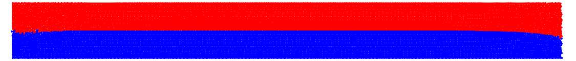
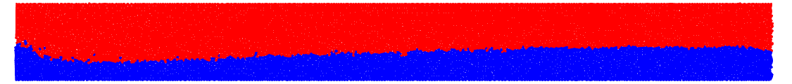
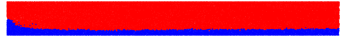
(a)

(b)

(c)

(d)

Figure 3: Case $L/\Delta r=312$ ($10000$ particles). (a) Evolution of the phases distribution at $t=1\leavevmode\nobreak\ \mathrm{s}$, $t=10\leavevmode\nobreak\ \mathrm{s}$ and $t=30\leavevmode\nobreak\ \mathrm{s}$ (not at scale). (b) Evolution of the number of particles with time. (c) Evolution of the outlet pressure with time. (d) Evolution of the inlet velocities with time.

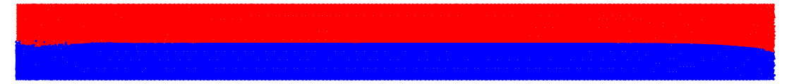
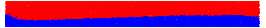
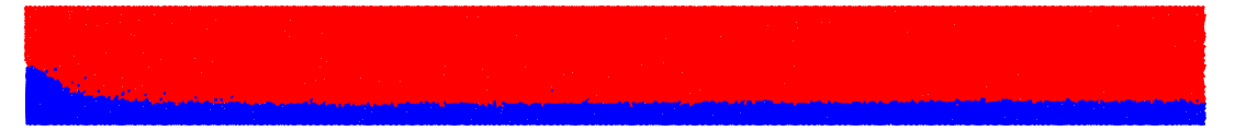
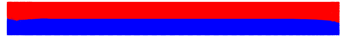
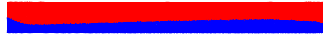
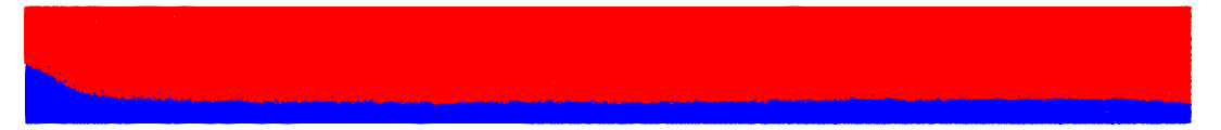
(a)

(b)

(c)

(d)

Figure 4: Case $L/\Delta r=444$ ($20000$ particles). (a) Evolution of the phases distribution at $t=1\leavevmode\nobreak\ \mathrm{s}$, $t=10\leavevmode\nobreak\ \mathrm{s}$ and $t=30\leavevmode\nobreak\ \mathrm{s}$ (not at scale). (b) Evolution of the number of particles with time. (c) Evolution of the outlet pressure with time. (d) Evolution of the inlet velocities with time.

(a)

(b)

(c)

(d)

Figure 5: Case $L/\Delta r=704$ ($50000$ particles). (a) Evolution of the phases distribution at $t=1\leavevmode\nobreak\ \mathrm{s}$, $t=10\leavevmode\nobreak\ \mathrm{s}$ and $t=30\leavevmode\nobreak\ \mathrm{s}$ (not at scale). (b) Evolution of the number of particles with time. (c) Evolution of the outlet pressure with time. (d) Evolution of the inlet velocities with time.

On Figures 3b, 4b and 5b, we note that the number of particles within the fluid flow is maintained throughout the simulation. The prescribed velocity at the inlet is reasonably well reproduced with an error that stays within $\pm 5\%$ for the light phase and $\pm 15\%$ for the heavy phase as shown on Figures 3d, 4d and 5d. The difference between the two phases is likely due to the relatively low number of particles (especially in the $y$ direction) and to the case geometry where the heavy phase has to push against the light phase causing more disturbances in the velocity field for the heavy phase. On the other hand, at the outlet, the prescribed pressure is very well recovered with an maximum error of $\pm 1\%$ as presented on Figures 3c, 4c and 5c. Besides, we observe that the errors are decreasing when the number of particles increases. These boundary conditions are not optimal but they perform reasonably well and are very easy to implement.

5 Results

There exists a large variety of flow regime maps to help characterize two-phase flow regime in pipes. For the particular case of horizontal pipes, one can mention Baker’s map [3] and Barnea’s map [4]. In this work, Taitel and Dukler’s map [61] has been used to predict flow regimes.

5.1 Validation for different flow regimes

We consider an horizontal pipe of diameter $D=1\mathrm{m}$ and length $L=10D$. The light phase and heavy phase are denoted with a $g$ and $l$ subscript respectively. The flow enters from the inlet (left) and is assumed to be stratified with equal volume fraction for each phase $\alpha_{g}=\alpha_{l}=0.5$. All the physical properties are summarized in Table 1. Using these properties, it is possible to plot the flow regime map, see Figure 7, and to pick four cases, one in each region, to be simulated. Those cases and their corresponding parameters are presented in Table 2 and marked by different symbols on Figure 7. All cases were simulated in 2D with three different resolutions $L/\Delta r=312$, $444$ and $704$ which corresponds approximately to $10000$, $20000$ and $50000$ particles. The simulation time was $30\leavevmode\nobreak\ \mathrm{s}$. At the inlet, each phase is injected with a constant velocity corresponding to its superficial velocity $u_{g,l}^{s}=\alpha_{g,l}u_{g,l}$. At the outlet, a constant pressure equal to the background pressure is prescribed. The initial setup is presented on Figure 6. The final two-flow patterns for the different cases, the evolution of the volume fraction with time at the outlet and the average pressure drop between both ends of the pipe is presented on Figures 8 to 12. In addition, the evolution of the velocity magnitude along the pipe’s length for each phase for the three particle resolutions considered is shown on Figures 13 and 14.

Figure 6: The initial configuration for all cases (not at scale).

Property Light Phase Heavy Phase Units Density ($\rho$) $1$ $5$ $\mathrm{k}\mathrm{g}\mathrm{/}\mathrm{m}^{3}$ Viscosity ($\mu$) $5\times 10^{-3}$ $1\times 10^{-2}$ $\mathrm{Pa}.\mathrm{s}$ Adiabatic index ($\gamma$) $7$ $7$ - Surface Tension ($\sigma^{nw}$) 0.001 $\mathrm{N}\mathrm{/}\mathrm{m}$ Contact Angle ($\theta_{c}$) 90 $\mathrm{\SIUnitSymbolDegree}$ Gravity ($g_{z}$) -1 $\mathrm{m}\mathrm{/}\mathrm{s}^{2}$

Table 1: Physical Properties

Property Case 1 Case 2 Case 3 Case 4 Units Flow pattern Mist Dispersed Intermittent Stratified - Superficial velocities ($u_{g}^{s}$,$u_{l}^{s}$) ($4.9$,$0.06$) ($0.05$,$8$) ($0.25$,$2$) ($0.7$,$0.06$) $\mathrm{m}\mathrm{/}\mathrm{s}$ Reynolds number ($Re=\frac{(u_{g}^{s}+u_{l}^{s})D}{\nu_{g}\alpha_{g}+\nu_{l}\alpha_{l}}$) $1417.14$ $2300$ $642.86$ $217.14$ - Friedel Pressure Drop Prediction ($\Delta p^{\text{Friedel}}$) $20.931$ $98.513$ $11.961$ $4.1$ $\mathrm{Pa}$

Table 2: Cases properties

Figure 7: Flow regime map adapted from [61]

For information purposes, Friedel correlation [17] has been used to evaluate the expected pressure drops for the four considered cases of Figure 7. These values reported in Table 2 are to be taken with caution as the Friedel correlation has proven not to be very reliable for rectangular channels, separated flows and/or viscous fluids [46, 69, 54]. Besides, on the same table, we also report the average Reynolds number for the considered geometry and flow conditions. Note that this is an average value. Depending on how it is computed, the Reynolds number could be locally much higher than the given value.

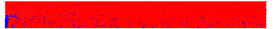
(a) $L/\Delta r=312$

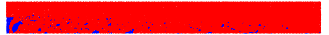
(b) $L/\Delta r=444$

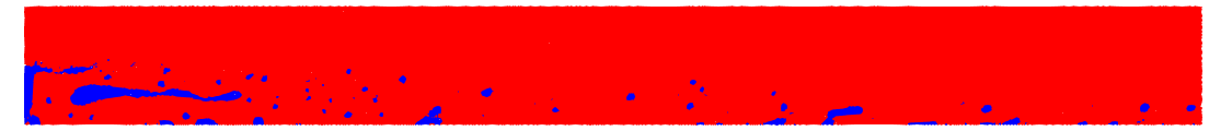
(c) $L/\Delta r=704$

(d) $L/\Delta r=312$

(e) $L/\Delta r=444$

(f) $L/\Delta r=704$

(g) $L/\Delta r=312$

(h) $L/\Delta r=444$

(i) $L/\Delta r=704$

Figure 8: Results for case 1 (Mist flow) : (a,b,c) Phases distribution at $t=30\leavevmode\nobreak\ \mathrm{s}$ (not at scale). (d,e,f) Evolution of the volume fractions at the outlet with time. (g,h,i) Evolution of the average pressure drop at the outlet with time.

On Figures 8a to 8c, one can observe that a mist flow pattern where the heavy phase is scattered by the light phase. It is confirmed by Figures 8d to 8f where we see that the light phase outlet volume fraction goes to $1$ after a transient period. Note that, in 3D, this mist pattern could be an annular flow under certain conditions. As the number of particles increases, Figures 8g to 8i show that the pressure drop level decreases and appears to stabilize around $\approx 100\leavevmode\nobreak\ \mathrm{Pa}$. This is higher than predicted by Friedel correlation. Note that turbulence is not included in the present model whereas the Reynolds number $Re$ is becoming turbulent and that the turbulent viscosity would contribute to stabilize the pressure field. For turbulence modeling in an SPH context, one can refer to [53, 67, 49] or [42].

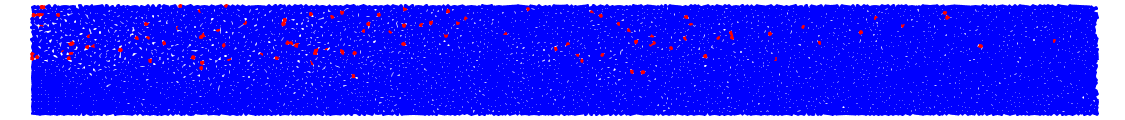
(a) $L/\Delta r=312$

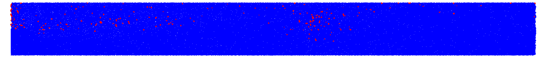
(b) $L/\Delta r=444$

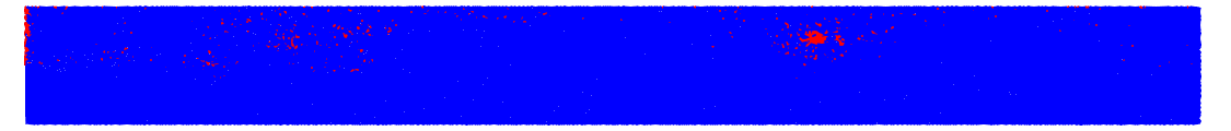
(c) $L/\Delta r=704$

(d) $L/\Delta r=312$

(e) $L/\Delta r=444$

(f) $L/\Delta r=704$

(g) $L/\Delta r=312$

(h) $L/\Delta r=444$

(i) $L/\Delta r=704$

Figure 9: Results for case 2 (Dispersed flow) : (a,b,c) Phases distribution at $t=30\leavevmode\nobreak\ \mathrm{s}$ (not at scale). (d,e,f) Evolution of the volume fractions at the outlet with time. (g,h,i) Evolution of the average pressure drop at the outlet with time.

On Figures 9a to 9c, pictures show a typical dispersed bubbly flow pattern where the light phase is spread-out by the heavy phase. Figures 9d to 9f support this claim as one can note that the heavy phase outlet volume fraction quickly goes to $1$ after a transient period. On Figures 9g to 9i, the pressure drop evolution with time presents large oscillations and its average level varies strongly with the particles’ resolution (from $\approx 500\leavevmode\nobreak\ \mathrm{Pa}$ to $\approx 0\leavevmode\nobreak\ \mathrm{Pa}$). It even becomes negative at some instants testifying the occurrence of important recirculation areas near the light phase inlet. It is also higher than what Friedel correlation predicts. However, as stated before, turbulence effects are not taken into account whereas the Reynolds number $Re$ is typically turbulent. We believe the turbulent viscosity would help to stabilize the pressure field.

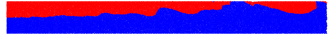
(a) $L/\Delta r=312$

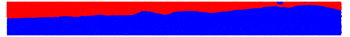
(b) $L/\Delta r=444$

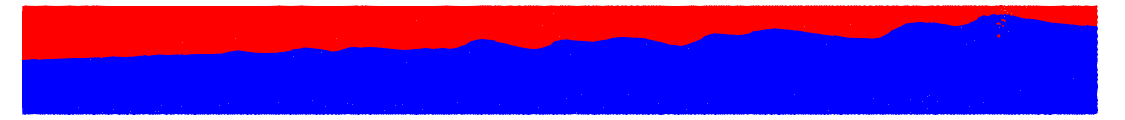
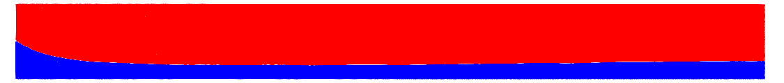
(c) $L/\Delta r=704$

(d) $L/\Delta r=312$

(e) $L/\Delta r=444$

(f) $L/\Delta r=704$

(g) $L/\Delta r=312$

(h) $L/\Delta r=444$

(i) $L/\Delta r=704$

Figure 10: Results for case 3 (Intermittent flow) : (a,b,c) Phases distribution at $t=30\leavevmode\nobreak\ \mathrm{s}$ (not at scale). (d,e,f) Evolution of the volume fractions at the outlet with time. (g,h,i) Evolution of the average pressure drop at the outlet with time.

On Figures 10a to 10c, we can see that an intermittent flow is established as expected. The intermittent character of the flow pattern is later confirmed by the volume fraction time series of Figures 10d to 10f where we can see that the light phase volume fraction is strongly oscillating between $0.25$ and $0$. It means that long bubbles are generated at a given frequency which corresponds to the definition of a slug flow. On Figures 10g to 10i, the pressure drop average level decreases when the number of particles increases, varying from $\approx 30\leavevmode\nobreak\ \mathrm{Pa}$ to $\approx 5\leavevmode\nobreak\ \mathrm{Pa}$. Friedel correlation predicts a pressure drop of $\approx 10\leavevmode\nobreak\ \mathrm{Pa}$ which is of the same order of magnitude. It goes under $0\leavevmode\nobreak\ \mathrm{Pa}$ during brief instants or during the transient phase because of the recirculation areas near the inlet. As shown on Figure 11, the intermittent flow presented in this plots would evolve towards a fully developed slug flow if the pipe was longer.

(a) $t=10\leavevmode\nobreak\ \mathrm{s}$

(b) $t=20\leavevmode\nobreak\ \mathrm{s}$

(c) $t=30\leavevmode\nobreak\ \mathrm{s}$

Figure 11: Phases distribution at selected instants for case 3 (Intermittent flow) with a pipe of $20\leavevmode\nobreak\ \mathrm{m}$ ($L/\Delta r=312$, not at scale).

(a) $L/\Delta r=312$

(b) $L/\Delta r=444$

(c) $L/\Delta r=704$

(d) $L/\Delta r=312$

(e) $L/\Delta r=444$

(f) $L/\Delta r=704$

(g) $L/\Delta r=312$

(h) $L/\Delta r=444$

(i) $L/\Delta r=704$

Figure 12: Results for case 4 (Stratified flow) : (a,b,c) Phases distribution at $t=30\leavevmode\nobreak\ \mathrm{s}$ (not at scale). (d,e,f) Evolution of the volume fractions at the outlet with time. (g,h,i) Evolution of the average pressure drop at the outlet with time.

Finally, on Figures 12a to 12c, we observe a fully developed stratified flow. Figures 12d to 12f show that the phase distribution is adjusting itself with time to reach a periodic steady state where the light phase volume fraction is $\approx 0.25$ and the heavy phase volume fraction is $\approx 0.75$. The pressure drop evolution presented on Figures 12g to 12i show much smaller oscillations than the other cases because the flow is evolving at a smaller speed. Its average level goes from $\approx 7.5\leavevmode\nobreak\ \mathrm{Pa}$ for the lowest resolution to $\approx 2.5\leavevmode\nobreak\ \mathrm{Pa}$ for the highest resolution. Friedel correlation gives an expected pressure drop of $\approx 4\leavevmode\nobreak\ \mathrm{Pa}$ which is of the same order of magnitude.

To sum up, one can observe that our current implementation of SPH is able to reproduce the two-phase flow patterns predicted by the flow map of Figure 7. Moreover, increasing the number of particles helps to reduce the pressure field oscillations while reproducing the same physics.

Moreover, on Figures 13 and 14, we provide plots showing the evolution of the velocity magnitude along the pipe length at $t=30\leavevmode\nobreak\ \mathrm{s}$ to verify that we do have a convergence of the velocity field when the number of particles increases. To obtain these plots, the velocity magnitude has been averaged along the pipe’s height for each phase. Note that, for the mist case (respectively the dispersed case), we do not show the heavy phase velocity (respectively the light phase velocity) since there are not enough particles of that phase to be considered within the pipe’s height. From a general point of view, what we observed is that, as the resolution increases, the velocity field tends to become more stable solution, presenting smaller oscillations and converging towards a steady state. This is particularly clear for the stratified case of Figures 13c and 14c. For the intermittent case, the velocity field also depends on the distribution of the bubbles of light phase. For instance, the peak on Figure 13b for the lowest resolution corresponds to the tail of the bubble of Figure 10a. This bubble just got formed and is self-adjusting its shape under the effect of surface tension, hence the peak in velocity. Concerning the mist and dispersed case of Figures 14a and 13a, we do not recover the prescribed velocity of the dominant phase at the inlet. It is because we average the velocity along the pipe’s height so that we include the recirculation areas at the entry which tends to reduce the magnitude of the velocity field. It is difficult to see a convergence of the pressure drops’ evolution when refining the resolution in Figures 8 to 12 because of the inherent pressure noise due to the weakly compressible SPH and more importantly because of the pressure waves reflections at the boundaries. However, we can visually observe that convergence in the velocity field especially for the steadier cases such as the stratified case.

(a) Case 2 (Dispersed flow)

(b) Case 3 (Intermittent flow)

(c) Case 4 (Stratified flow)

Figure 13: Heavy phase velocity magnitude along the pipe length at $t=30\leavevmode\nobreak\ \mathrm{s}$ in function of the particle resolution.

(a) Case 1 (Mist flow)

(b) Case 3 (Intermittent flow)

(c) Case 4 (Stratified flow))

Figure 14: Light phase velocity magnitude along the pipe length at $t=30\leavevmode\nobreak\ \mathrm{s}$ in function of the particle resolution.

5.2 Transitions

Using the same geometry, fluid properties and flow map as in the previous section, we picked four different paths from one flow pattern to the other. For each path, we simulated four different cases that are marked with different symbols on Figure 15 and the corresponding parameters are shown on Table 3. All cases were simulated in 2D with a particle resolution of $L/\Delta r=312$ which corresponds approximately to $10000$ particles. The simulation time was $30\leavevmode\nobreak\ \mathrm{s}$. At the inlet, each phase is injected with a constant velocity corresponding to its superficial velocity $u_{g,l}^{s}=\alpha_{g,l}u_{g,l}$. At the outlet, a constant pressure equal to the background pressure is prescribed. The final two-flow patterns for the different cases, the evolution of the volume fraction with time at the outlet and the average pressure drop between both ends of the pipe are shown on Figures 16 to 19.

Property Path 1 Path 2 Path 3 Path 4 Units Flow pattern Stratified to Mist Mist to Intermittent Stratified to Intermittent Intermittent to Dispersed - Superficial velocities $\#1$ ($u_{g}^{s}$,$u_{l}^{s}$) ($1.0$,$0.06$) ($3.0$,$0.4$) ($0.3$,$0.15$) ($0.22$,$3.0$) $\mathrm{m}\mathrm{/}\mathrm{s}$ Superficial velocities $\#2$ ($u_{g}^{s}$,$u_{l}^{s}$) ($1.5$,$0.06$) ($2.0$,$0.8$) ($0.25$,$0.25$) ($0.15$,$4.0$) $\mathrm{m}\mathrm{/}\mathrm{s}$ Superficial velocities $\#3$ ($u_{g}^{s}$,$u_{l}^{s}$) ($2.5$,$0.06$) ($1.0$,$1.2$) ($0.2$,$0.6$) ($0.1$,$6.0$) $\mathrm{m}\mathrm{/}\mathrm{s}$ Superficial velocities $\#4$ ($u_{g}^{s}$,$u_{l}^{s}$) ($3.5$,$0.06$) ($0.5$,$1.6$) ($0.2$,$1.0$) ($0.07$,$7.0$) $\mathrm{m}\mathrm{/}\mathrm{s}$ Reynolds number $\#1$ ($Re=\frac{(u_{g}^{s}+u_{l}^{s})D}{\nu_{g}\alpha_{g}+\nu_{l}\alpha_{l}}$) $302.86$ $971.43$ $128.57$ $920.00$ - Reynolds number $\#2$ ($Re=\frac{(u_{g}^{s}+u_{l}^{s})D}{\nu_{g}\alpha_{g}+\nu_{l}\alpha_{l}}$) $445.71$ $800.00$ $142.86$ $1185.71$ - Reynolds number $\#3$ ($Re=\frac{(u_{g}^{s}+u_{l}^{s})D}{\nu_{g}\alpha_{g}+\nu_{l}\alpha_{l}}$) $731.43$ $228.57$ $642.86$ $1742.86$ - Reynolds number $\#4$ ($Re=\frac{(u_{g}^{s}+u_{l}^{s})D}{\nu_{g}\alpha_{g}+\nu_{l}\alpha_{l}}$) $1017.14$ $600.00$ $342.86$ $2020.00$ -

Table 3: Cases properties for the different paths

Figure 15: Four different paths from one flow pattern to another.

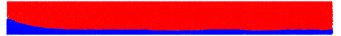
(a) $\#1$

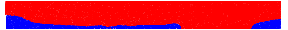
(b) $\#2$

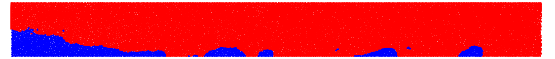
(c) $\#3$

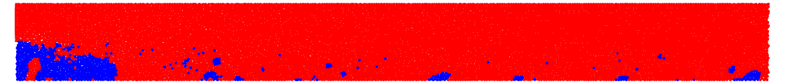
(d) $\#4$

(e) $\#1$

(f) $\#2$

(g) $\#3$

(h) $\#4$

(i) $\#1$

(j) $\#2$

(k) $\#3$

(l) $\#4$

Figure 16: Results for path 1 (Stratified to Mist) : (a,b,c,d) Phases distribution at $t=30\leavevmode\nobreak\ \mathrm{s}$ (not at scale). (e,f,g,h) Evolution of the volume fractions at the outlet with time. (i,j,k,l) Evolution of the average pressure drop at the outlet with time.

On Figures 16a to 16d, the transition from a stratified to a mist flow (path 1) is shown. As the superficial velocity of the light phase increases from case $\#1$ to case $\#4$, the volume fraction of the light phase is going to $\approx 1$ while the volume fraction of the heavy fluid is going to $0$. In between, we can see that the heavy fluid layer is divided in pieces until being completely dispersed by the light phase. Volume fractions plots of Figures 16e to 16h show that the transition between the two patterns goes through a phase of intermittent flow where the heavy phase layer dislocates forming drops. On Figures 16i to 16l, the pressure drop level increases from $\approx 10\leavevmode\nobreak\ \mathrm{Pa}$ to $\approx 150\leavevmode\nobreak\ \mathrm{Pa}$ and present stronger and stronger oscillations while transitioning to the mist flow pattern.

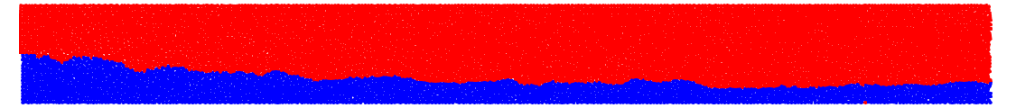
(a) $\#1$

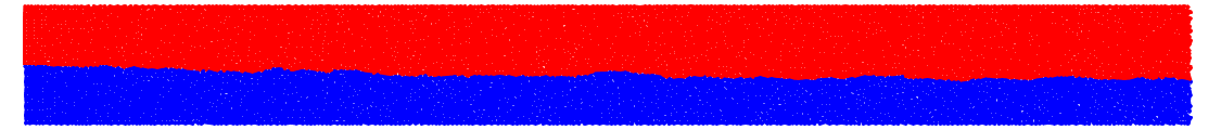
(b) $\#2$

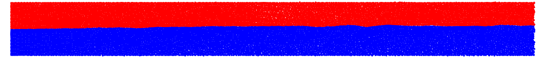
(c) $\#3$

(d) $\#4$

(e) $\#1$

(f) $\#2$

(g) $\#3$

(h) $\#4$

(i) $\#1$

(j) $\#2$

(k) $\#3$

(l) $\#4$

Figure 17: Results for path 2 (Mist to Intermittent) : (a,b,c,d) Phases distribution at $t=30\leavevmode\nobreak\ \mathrm{s}$ (not at scale). (e,f,g,h) Evolution of the volume fractions at the outlet with time. (i,j,k,l) Evolution of the average pressure drop at the outlet with time.

The transition from mist flow to intermittent flow (path 2) is presented on Figures 17a to 17d. From a quasi-mist flow in case $\#1$, we see that, as the heavy phase superficial velocity increases, the fluid becomes wavy and then evolves towards an intermittent flow. This is magnified by the volume fractions evolution plots of Figures 17e to 17h where we see that the light phase dominant in case $\#1$ whereas the heavy phase is dominant in case $\#4$. In all four cases, volume fractions are showing significant oscillations so that it is not obvious to qualify where the flow becomes really intermittent. This supports the well-known fact that flow maps are only an indicative tool and that the transition lines are not lines but smooth transitions areas. Concerning the pressure drop evolution of Figures 17i to 17l, we can see that the average level drops from $\approx 125\leavevmode\nobreak\ \mathrm{Pa}$ to $\approx 25\leavevmode\nobreak\ \mathrm{Pa}$. The case $\#3$ is particular since in that case, superficial velocities and volume fractions are the same, therefore it is a very stable case where the pressure drop oscillations are the smallest.

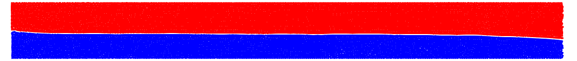
(a) $\#1$

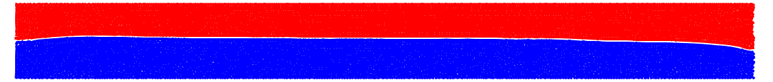
(b) $\#2$

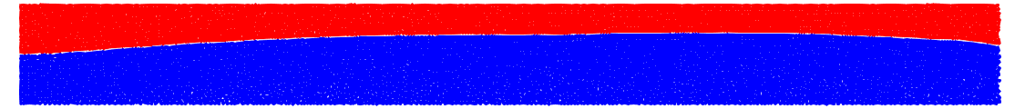
(c) $\#3$

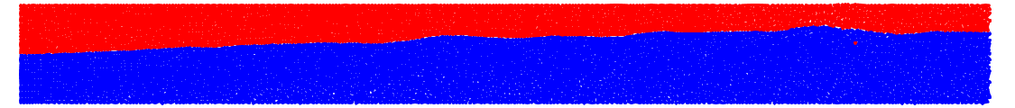
(d) $\#4$

(e) $\#1$

(f) $\#2$

(g) $\#3$

(h) $\#4$

(i) $\#1$

(j) $\#2$

(k) $\#3$

(l) $\#4$

Figure 18: Results for path 3 (Stratified to Intermittent) : (a,b,c,d) Phases distribution at $t=30\leavevmode\nobreak\ \mathrm{s}$ (not at scale). (e,f,g,h) Evolution of the volume fractions at the outlet with time. (i,j,k,l) Evolution of the average pressure drop at the outlet with time.

On Figures 18a to 18d, we present the phases distribution for the transition from a stratified flow pattern to an intermittent flow pattern. As the heavy phase velocity increases, the heavy phase becomes dominant and the interface with the light phase is more and more wavy near the outlet which prefigures the emergence of an intermittent flow. Volume fractions plots shown on Figures 18e to 18h support that observation as the amplitudes of their oscillations are increasing when we move towards the intermittent flow pattern. On Figures 18i to 18l, one can note that the pressure drops evolutions behave similarly and their average level increases from $\approx 4\leavevmode\nobreak\ \mathrm{Pa}$ to $\approx 8\leavevmode\nobreak\ \mathrm{Pa}$.

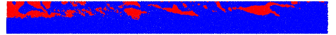
(a) $\#1$

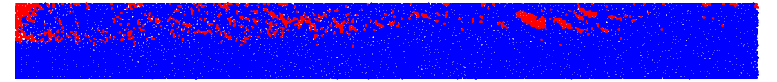
(b) $\#2$

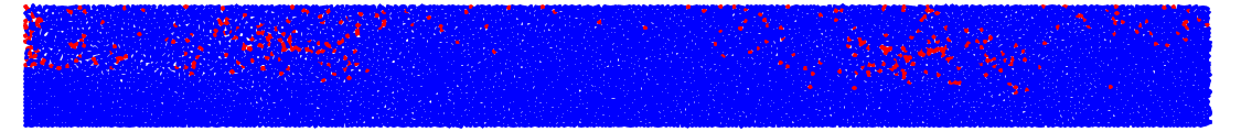
(c) $\#3$

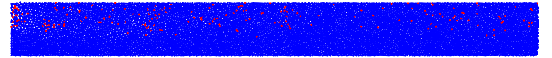
(d) $\#4$

(e) $\#1$

(f) $\#2$

(g) $\#3$

(h) $\#4$

(i) $\#1$

(j) $\#2$

(k) $\#3$

(l) $\#4$

Figure 19: Results for path 4 (Intermittent to Dispersed) : (a,b,c,d) Phases distribution at $t=30\leavevmode\nobreak\ \mathrm{s}$ (not at scale). (e,f,g,h) Evolution of the volume fractions at the outlet with time. (i,j,k,l) Evolution of the average pressure drop at the outlet with time.

The transition from intermittent flow to dispersed flow is presented on Figures 19a to 19d. The flow pattern evolves from a disturbed intermittent flow that we could qualify of plug flow towards a dispersed flow as the heavy phase velocity increases. On Figures 19e to 19h, on can observe that volume fractions time series are initially very unstable which is characteristic of an intermittent flow. The light phase and heavy phase volume fractions are going to $\approx 0$ and $\approx 1$ respectively as the dispersed flow pattern emerges. Concerning the pressure drops of Figures 19i to 19l, as expected, it increases from $\approx 75\leavevmode\nobreak\ \mathrm{Pa}$ to $\approx 400\leavevmode\nobreak\ \mathrm{Pa}$ with growing oscillations.

To conclude, we have explored the flow map of Figure 15 by simulating several cases located around the transitions from one pattern to the other. We observed that the transition areas are not lines but in fact smooth bands. Also, it appears that the intermittent flow area gathers different patterns such as wavy flows (in the lower part), slug flows (in the center) and even plug flows (in the upper area). The pressure drop plots are providing useful information on the pressure field but are showing strong variations which are due to the use of the weakly compressible formulation. This approach is known to generate disturbances in the pressure calculations because of density and pressure are linked through an equation of state (2.3). A truly incompressible SPH formulation would likely improve this aspect. See [27, 31] for multiphase incompressible SPH models. Besides, the inlet, outlet and wall boundary conditions that we have used are known to introduce spurious waves in the flow. We believe that implementing more accurate boundary conditions based on analytical considerations [15] and adapted to inlet/outlet for multiphase flows could also improve the quality of the results. Nevertheless, we think that these results show that SPH could be a complementary tool to study the emergence of intermittent flow patterns in pipes in industrial applications.

5.3 Applied cases with high density and viscosity ratios

In order to further demonstrate the potential of SPH to model intermittent flows, we have simulated two applied cases. The fluids considered for these cases are generic oil and natural gas whose properties are indicated in Table 4. The two different geometries corresponding to a hydrodynamic slugging case and a terrain slugging case are shown on Figure 20 and are discretized with resolutions $L/\Delta r=634$ ($\approx 10000$ particles) and $L/\Delta r=687$ ($\approx 15000$ particles) respectively. Simulation times are $0.05\mathrm{s}$ and $0.25\mathrm{s}$ respectively. Fluids are injected with superficial velocities and volume fractions given in Table 5. Note that we have chosen to work with a micro-geometry for computational and time constraints while trying to preserve realistic proportions. Phases distributions for both cases are shown on Figures 21 and 22.

(a)

(b)

Figure 20: Geometrical configurations for the two applied cases (not at scale). (a) Hydrodynamic slugging. (b) Terrain slugging.

Property Gas Phase Oil Phase Units Density ($\rho$) $1.6454$ $702.6926$ $\mathrm{k}\mathrm{g}\mathrm{/}\mathrm{m}^{3}$ Viscosity ($\mu$) $1.27\times 10^{-5}$ $4.19\times 10^{-4}$ $\mathrm{Pa}.\mathrm{s}$ Adiabatic index ($\gamma$) $1.4$ $7$ - Surface Tension ($\sigma^{nw}$) 0.02139 $\mathrm{N}\mathrm{/}\mathrm{m}$ Contact Angle ($\theta_{c}$) 90 $\mathrm{\SIUnitSymbolDegree}$ Gravity ($g_{z}$) -9.81 $\mathrm{m}\mathrm{/}\mathrm{s}^{2}$

Table 4: Physical Properties

Property Hydrodynamic slugging Terrain slugging Units Volume fractions ($\alpha_{g}$,$\alpha_{l}$) ($0.25$,$0.75$) ($0.25$,$0.75$) $\mathrm{m}\mathrm{/}\mathrm{s}$ Superficial velocities ($u_{g}^{s}$,$u_{l}^{s}$) ($0.35$,$0.76125$) ($0.35$,$0.76125$) $\mathrm{m}\mathrm{/}\mathrm{s}$

Table 5: Cases Properties

Figure 21: Phases distribution for the hydrodynamic slugging case (not at scale). From top to bottom, at $t=0\leavevmode\nobreak\ \mathrm{s}$, $0.01\leavevmode\nobreak\ \mathrm{s}$, $0.02\leavevmode\nobreak\ \mathrm{s}$, $0.025\leavevmode\nobreak\ \mathrm{s}$, $0.026\leavevmode\nobreak\ \mathrm{s}$, $0.0275\leavevmode\nobreak\ \mathrm{s}$, $0.03\leavevmode\nobreak\ \mathrm{s}$, $0.035\leavevmode\nobreak\ \mathrm{s}$, $0.04\leavevmode\nobreak\ \mathrm{s}$ and $0.05\leavevmode\nobreak\ \mathrm{s}$

On Figure 21, it is possible to observe the typical formation process of a hydrodynamic slug. First, from $t=0\leavevmode\nobreak\ \mathrm{s}$ to $t=0.025\leavevmode\nobreak\ \mathrm{s}$, waves begin to grow. At $t=0.026\leavevmode\nobreak\ \mathrm{s}$, one the waves’ crest is high enough to reach the top of pipe : a slug is formed. From $t=0.0275\leavevmode\nobreak\ \mathrm{s}$ to $t=0.03\leavevmode\nobreak\ \mathrm{s}$, other waves reach the top of the pipe forming new slugs. After that, one can note that some slugs see their length reduced and their height increased until occupying the whole pipe’s height. This example confirms that SPH can reproduce the dynamics of slug flows with high viscosity and density ratios (here $\approx 32$ and $\approx 427$ respectively).

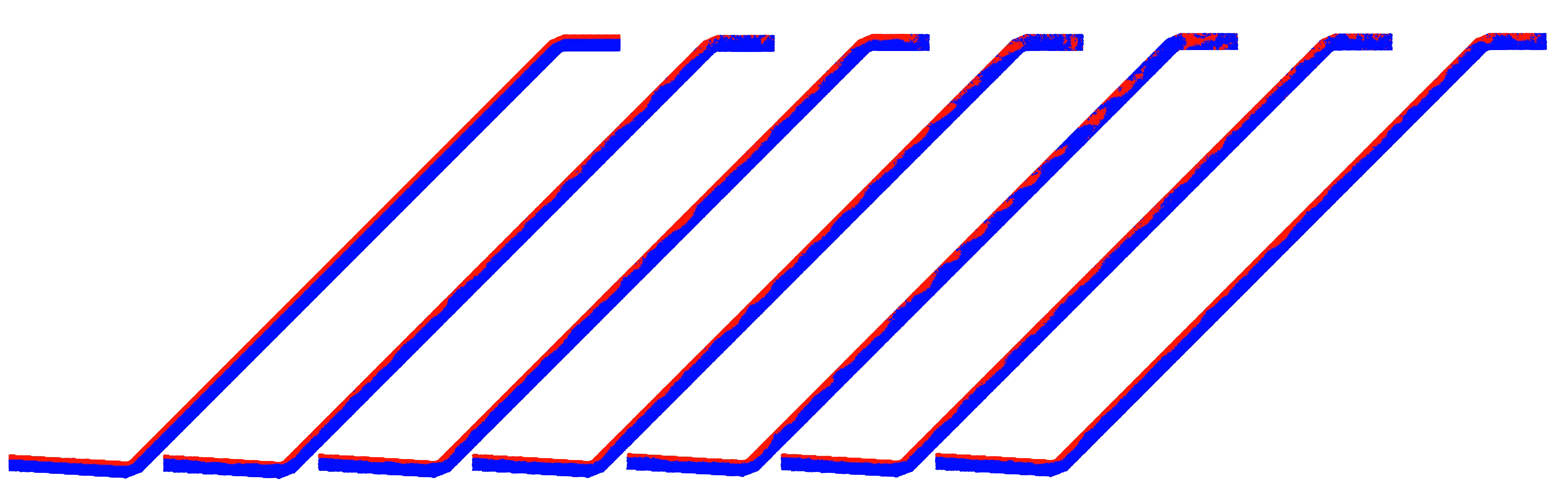
(a)

(b)

(c)

Figure 22: (a) Phases distribution for the terrain slugging case. From left to right, at $t=0\leavevmode\nobreak\ \mathrm{s}$, $0.05\leavevmode\nobreak\ \mathrm{s}$, $0.1\leavevmode\nobreak\ \mathrm{s}$, $0.13\leavevmode\nobreak\ \mathrm{s}$, $0.188\leavevmode\nobreak\ \mathrm{s}$, $0.2\leavevmode\nobreak\ \mathrm{s}$ and $0.25\leavevmode\nobreak\ \mathrm{s}$ (b) Evolution of the volume fractions at the outlet with time. (c) Fourier transform of the gas phase volume fraction time series (in red on (b))

On Figure 22, we present the results of a "riser-like" case where the oil and gas mixture extracted from the reservoir is lifted from the sea ground to the land. A slug flow does not have the required distance to grow in the initial descending part of the pipe. However, under the effect of gravity, slugging begins to occur in the ascending part of the pipe. The evolution of volume fractions at the outlet of Figure 22b shows strong oscillations as expected in a slug flow. When performing a Fourier transform analysis on the gas phase volume fraction evolution as presented on Figure 22c, one can see that one frequency clearly dominates, thus suggesting that the slug frequency in that particular case geometry would be around $226\leavevmode\nobreak\ \mathrm{Hz}$.

6 Conclusion

In this paper, we have combined ideas from [58, 2] to present inlet/outlet boundary conditions for multiphase flows in SPH. These boundary conditions have then been used to simulate intermittent flows in pipes. First, we have shown that our SPH implementation is able to reproduce four different flow regimes (mist flow, dispersed flow, intermittent flow and stratified flow) predicted by Taitel and Dukler’s flow map. Then, we focused on the transition processes from one flow pattern to another : stratified to mist, stratified to intermittent, mist to intermittent and intermittent to dispersed.

From theses simulations, we have confirmed that SPH has a strong potential to model two-phase flow in pipes and to understand how one pattern evolves into another one. However, we believe that our boundary conditions, although simple and easy to implement, are not optimal and that a semi-analytic approach [15] could improve the quality of the results. Similarly, pressure drops of our simulations have reasonable levels that correspond to flow velocities but are also presenting large oscillations due to the weakly compressible approach. A truly incompressible formulation based on a Poisson solver could remediate this issue. Finally, we have simulated two cases of hydrodynamic slugging and terrain slugging involving high density and viscosity ratios to demonstrate the applicability of multiphase SPH to more realistic problems.

Albeit satisfactory, our results could certainly be improved. To this end, three main tasks can be identified. First, it would be interesting to verify if including the turbulence effects and increasing the number of particles would stabilize the pressure field, especially for high Reynolds cases. Then, it is needed to clarify the influence of shifting and interface correction on the results through a parameter study. Finally, a comparison with results obtained from another numerical method or from a commercial software would be mandatory to further assess the potential interest of SPH in slugging modeling. In addition, recently proposed multiphase SPH models such as [23] could possibly enhance the quality of the simulations.

Although in general slower than other numerical methods, this study intended to show that SPH, thanks to its ease of handling interface dynamics, could be used in industrial applications to model intermittent flows and in particular slug and plug flows with reliable results. This work hopes to serve as a basis on which to build more complex SPH models including turbulence effects to capture the flow behavior with more accuracy.

References

Appendix A Validation Cases

For all the following validation cases, no kernel gradient correction or shifting or interface correction were used.

A.1 Lid-driven Cavity Flow

The goal of this section is to validate the implementation of SPH for the single phase Navier-Stokes case. The test case chosen for this purpose is the well-known 2D lid-driven cavity flow problem shown on Figure 23. This is a common problem in the fluid mechanics community and numerous reference solutions performed with different numerical methods are available in the literature. In this case, we use Ghia et al. solution as a reference [20].

Figure 23: The 2D Lid-driven Cavity Flow problem

The Reynolds number for this problem is defined as follows $Re=\frac{U_{\text{lid}}L}{\nu}$ where $U_{\text{lid}}$ is the velocity of the imposed at the top boundary, $\nu$ is the kinematic viscosity and $L$ is the characteristic length of the problem. The simulations were performed for $Re=100$ and $1000$ and for $50\times 50$, $100\times 100$ and $200\times 200$ particles. The density is set to $1000\leavevmode\nobreak\ \mathrm{k}\mathrm{g}\mathrm{/}\mathrm{m}^{3}$, the velocity of the lid is $U_{\text{lid}}=1\leavevmode\nobreak\ \mathrm{m}\mathrm{/}\mathrm{s}$, the domain is $L_{x}\times L_{y}=1\leavevmode\nobreak\ \mathrm{m}\times 1\leavevmode\nobreak\ \mathrm{m}$ and the viscosity $\nu$ is adjusted to reach the desired Reynolds number. $\gamma=7.0$ for both fluids.

The velocity boundary condition at the top boundary has been applied using the procedure described in section 4. For the other boundaries, a no-slip boundary conditions has been applied. The simulations are terminated when a steady state is reached (i.e. $\sqrt{\sum_{a}\frac{\lvert\rho_{a}^{n+1}-\rho_{a}^{n}\rvert}{\rho_{a}^{n}}}<1e^{-2}$ or after $60\leavevmode\nobreak\ \mathrm{s}$ of real simulated time).

A.1.1 $Re=100$

(a)

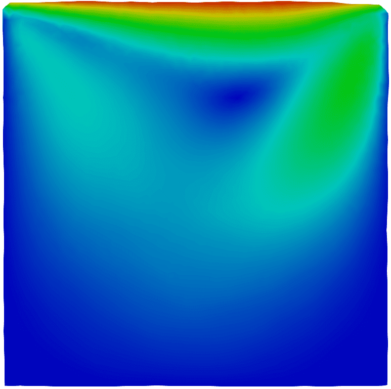
(b) $50\times 50$

(c)

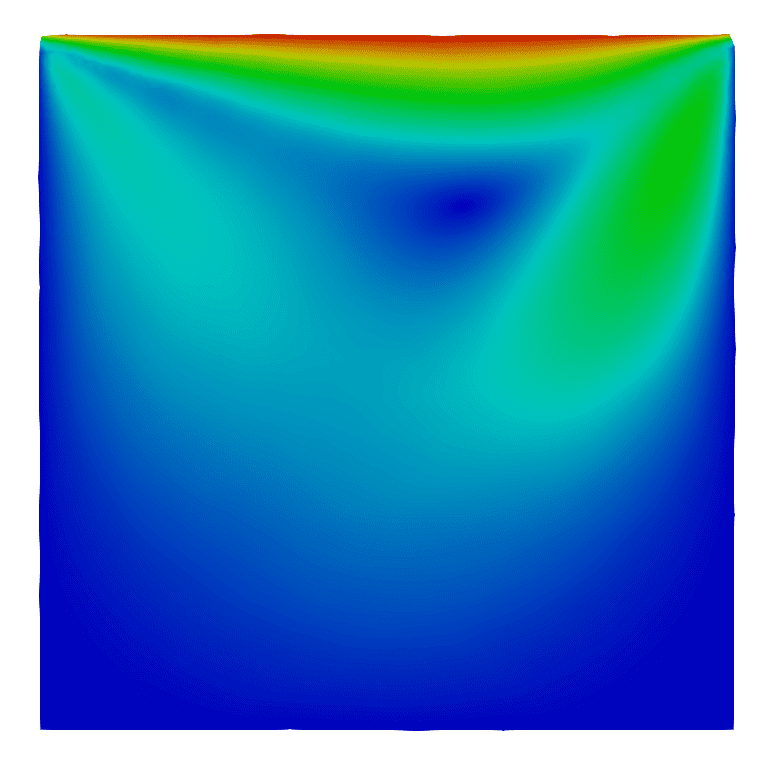
(d) $100\times 100$

(e)

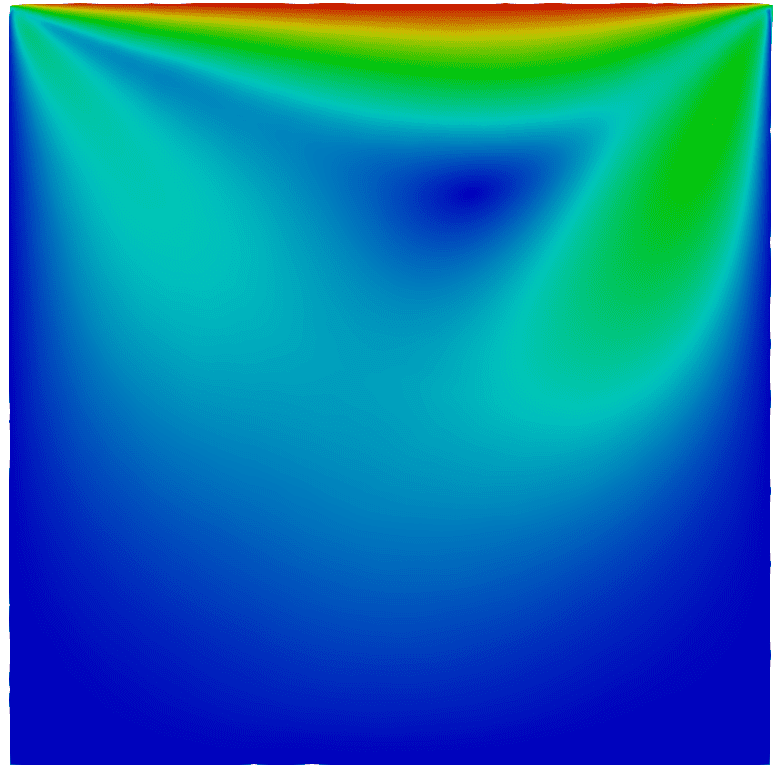
(f) $200\times 200$

(g) $50\times 50$

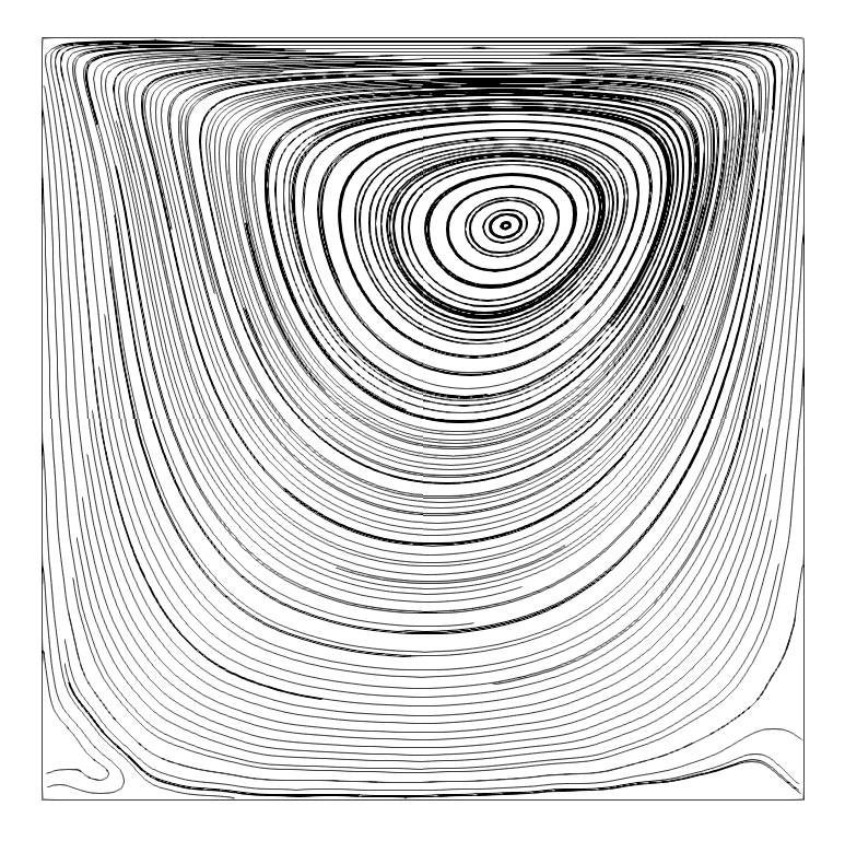
(h) $100\times 100$

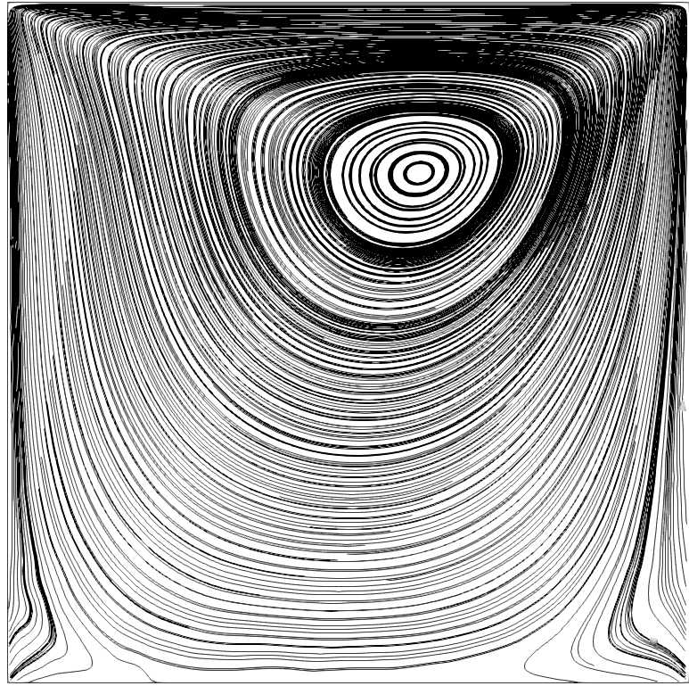
(i) $200\times 200$

Figure 24: Steady-state results for $Re=100$ showing the velocity distribution (left) and the corresponding streamlines (right)

(a)

(b)

(c)

(d)

Figure 25: $Re=100$

When $Re=100$, SPH is able to reproduce the velocity field accurately. The maximum error is reached at the boundaries but remains low ($\lesssim 2\%$ for the $200\times 200$ case close to the boundaries, figure not shown here). On Figure 25, the $L_{2}$ norm of the error with respect to the reference solution has been plotted in function of the number of particles in log scale. We observe a linear "mesh" convergence for the both velocity fields when the particle resolution increases. The convergence rate is $\approx 0.1$.

Concerning the spatial distribution of the flow, the theory predicts the appearance of two vortexes at the two bottom corners of the domain. As shown on Figure 24, SPH is not able to reproduce those two vertexes but instead has flow perturbations in the concerned areas.

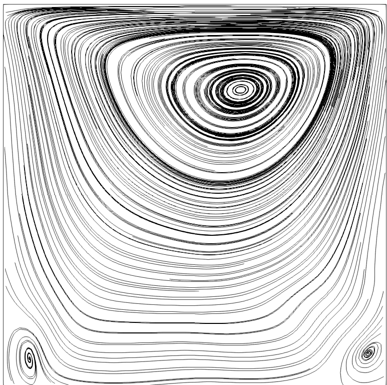
(a) $50\times 50$ - $t=2.48s$

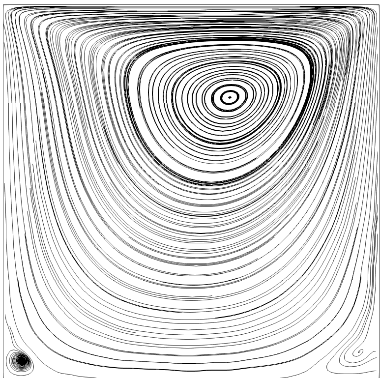
(b) $100\times 100$ - $t=46.66s$

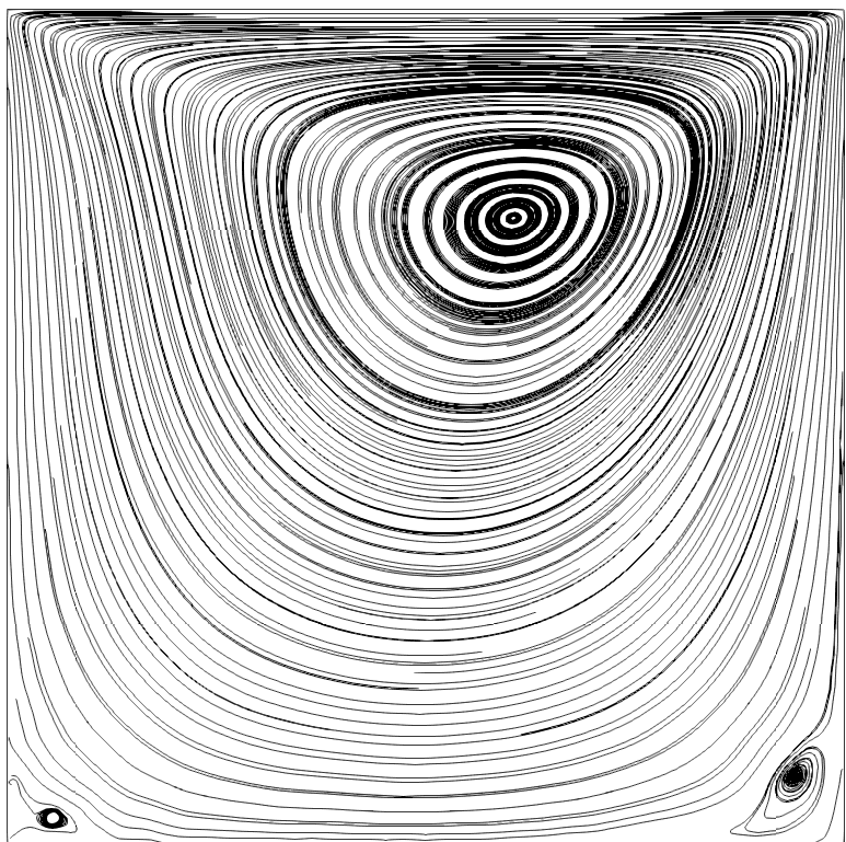
(c) $200\times 200$ - $t=54.31s$

Figure 26: Streamlines for $Re=100$ at selected timesteps

On Figure 26, one can note that the two expected vertexes at the corners are in fact appearing during the SPH simulations but they are highly unstable. They keep forming (together or independently) and vanishing as the simulation progresses. It indicates that SPH captures an instability in the correct areas but fails to reach a steady state thus the formation of spurious perturbations. Those vertexes being of small intensity, their formation is likely to be affected by boundary conditions.

A.1.2 $Re=1000$

(a)

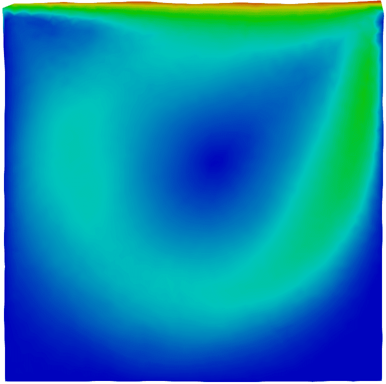
(b) $50\times 50$

(c)

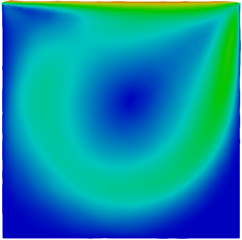
(d) $100\times 100$

(e)

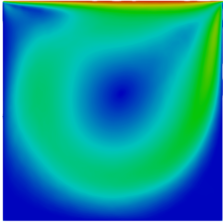
(f) $200\times 200$

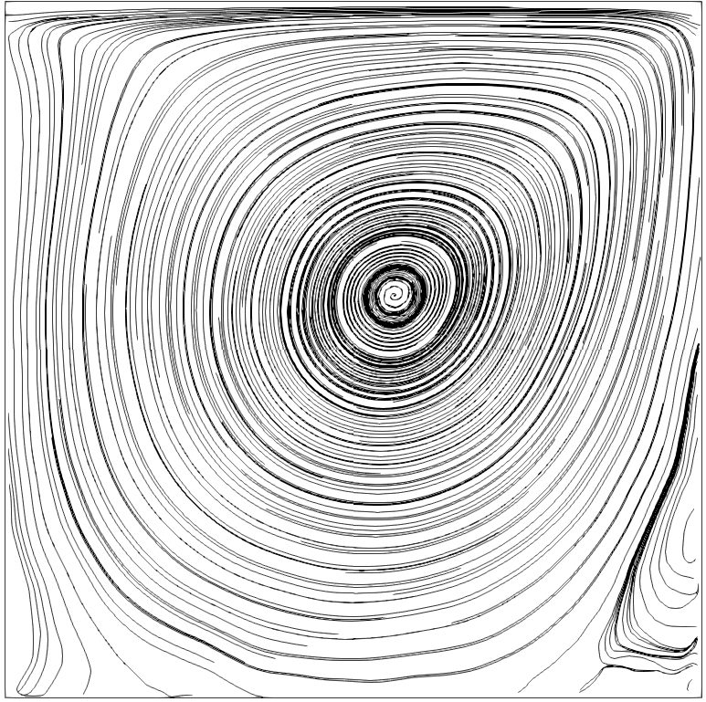
(g) $50\times 50$

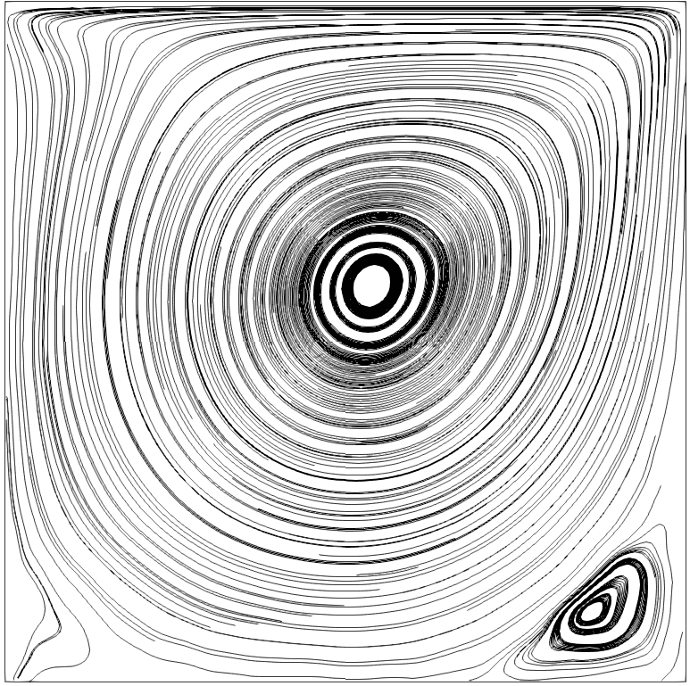
(h) $100\times 100$

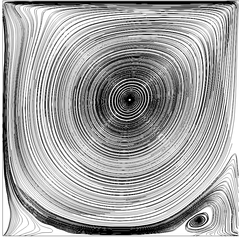
(i) $200\times 200$

Figure 27: SPH steady-state results for $Re=1000$ showing the velocity distribution (left) and the corresponding streamlines (right)

(a)

(b)

(c)

(d)

Figure 28: $Re=1000$

For $Re=1000$, at the highest resolution, SPH gives an error of $\approx 15\%$ at the right boundary and $\leq 6\%$ in the interior of the cavity (figure not shown here). As in the previous case, we observe an approximate linear "mesh" convergence for both velocity fields as shown on Figure 28. The convergence rate is $\approx 0.25$.

For this Reynolds number, it can be seen on Figure 27 that SPH is capable of generating a vertex pattern at the bottom right corner for the two highest resolutions but it is unstable for the smallest resolution. Moderate deviations of the flow indicating a potential growing vortex can be seen at the bottom left corner. When computing the streamlines for selected timesteps of the SPH simulations as shown on Figure 29, it is seen that all three resolutions are generating vertexes in the correct spots but only the $200\times 200$ case manage to stabilize one at the bottom right corner.

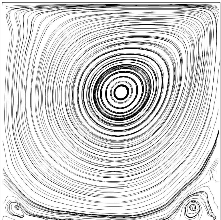
(a) $50\times 50$ - $t=52.83\leavevmode\nobreak\ \mathrm{s}$

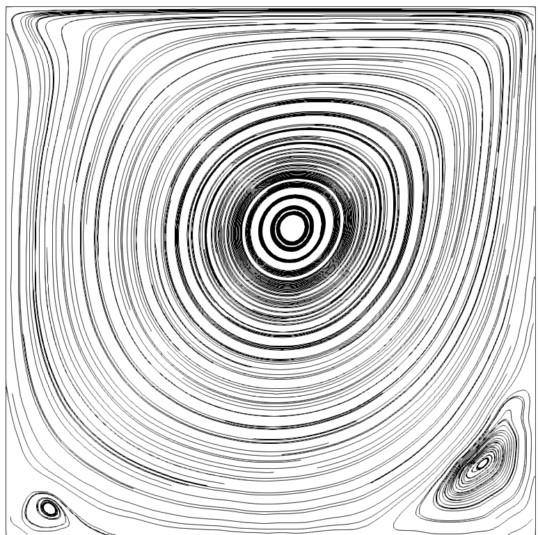
(b) $100\times 100$ - $t=50.5\leavevmode\nobreak\ \mathrm{s}$

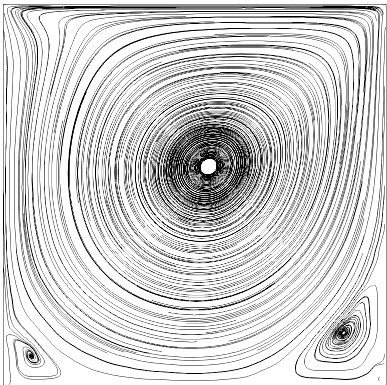
(c) $200\times 200$ - $t=52.6\leavevmode\nobreak\ \mathrm{s}$

Figure 29: Streamlines for $Re=1000$ at selected timesteps

A.2 Laplace’s law

In this section, the objective is to validate the implementation of the surface tension model described in section 2.2. The standard square to droplet test case is simulated and when a steady state is reached, the pressure difference between the exterior and the interior of the bubble is measured and compared to Laplace’s formula

$$\Delta P=\frac{\sigma}{R}=\frac{\sigma\sqrt{\pi}}{a}$$ (A.1)

with $\Delta P$ the pressure difference, $\sigma$ the surface tension coefficient, $R$ the bubble’s radius and $a$ the length of the edge of the initial square droplet.

Simulations are performed for three different resolution: $60\times 60$, $100\times 100$ and $200\times 200$ particles. The density and viscosity ratios are equal to one. The surface tension coefficient is $\sigma=22.5\leavevmode\nobreak\ \mathrm{N}\mathrm{/}\mathrm{m}$. The whole domain is $1\leavevmode\nobreak\ \mathrm{m}\times 1\leavevmode\nobreak\ \mathrm{m}$ and the edge of the initial square droplet is $a=0.6\leavevmode\nobreak\ \mathrm{m}$. $\gamma=7.0$ for both fluids. The time is normalized by $t_{\sigma}=\sqrt{\rho a^{3}/\sigma}$. This test case and its parameters values are taken from [55]. On Figure 30, one can observe the deformation from a square to a circle in the $60\times 60$ case whereas on Figure 31, pressure profiles are plotted. The error is $\leq 5\%$ at the center of the bubble for $60\times 60$ case and $\leq 1.5\%$ for the $200\times 200$ case, but the highest resolution exhibits a steeper pressure profile in accordance with the analytical profile. Moreover, this test case allows us to confirm that the small structures (bubbles or drops made of a handful of particles) observed in Figures 8 and 9 for example are not discretized enough to ensure a realistic behavior [57]. The minimum number of particles for a droplet or a bubble to behave properly has yet to be exactly determine but a minimum number of $400$ particles appears necessary (with the current formulation) to recover Laplace’s law with an error around $5\%$ and a reasonably steep pressure profile.

(a) $t/t_{\sigma}=0.2$

(b) $t/t_{\sigma}=0.6$

(c) $t/t_{\sigma}=1.5$

Figure 30: Evolution of the square to droplet deformation at selected timesteps

Figure 31: Pressure profiles in the steady state

A.3 Contact Angle

In order to extended the validation of the surface tension model described in section 2.2, a test to evaluate the ability of the model to prescribe a contact angle between a wetting phase, a non-wetting phase and a solid phase is performed. Simulations are done with $60\times 60$ particles. The density and viscosity ratios are both equal to one. $\gamma=7.0$ for both fluids. The surface tension coefficient between the wetting and non-wetting phase is $\sigma^{nw}=100\leavevmode\nobreak\ \mathrm{N}\mathrm{/}\mathrm{m}$ whereas the one between the wetting and the solid phase is set to $\sigma^{sw}=0\leavevmode\nobreak\ \mathrm{N}\mathrm{/}\mathrm{m}$ and the one between the non-wetting and the solid phase $\sigma^{sn}$ is adjusted to prescribed the desired contact angle $\theta^{\text{prescribed}}_{c}$ using the Young-Laplace equation

$$\theta_{c}=\frac{\sigma^{sw}-\sigma^{sn}}{\sigma^{nw}}$$ (A.2)

The whole domain is $1\leavevmode\nobreak\ \mathrm{m}\times 1\leavevmode\nobreak\ \mathrm{m}$ and the edge of the initial rectangle droplet is $0.6\leavevmode\nobreak\ \mathrm{m}\times 0.3\leavevmode\nobreak\ \mathrm{m}$. At steady state, the observed contact angle $\theta^{\text{observed}}_{c}$ is measured and reported in Figure 32. The coefficient of determination is $0.9894$ confirming that the model can accurately reproduce a prescribed contact angle.

Figure 32: Different measured contact angles

A.4 Capillary Rise

The well-known capillary rise problem is a simple test case to further verify the ability of the model to reproduce contact line dynamics. The problem is described in Figure 33. It consists of two fluids, one on top of the other. Two vertical parallel plates are immersed in the fluids. Thanks to the action of surface tension, the lower fluid will rise along the parallel plates forming a meniscus between them. The lower liquid height reached at steady state follows Jurin’s law

$$H_{\text{J}}=\frac{2\sigma^{nw}\cos{\theta_{c}}}{(\rho_{w}-\rho_{n})gD}$$ (A.3)

with $\sigma^{nw}$ the surface tension coefficient between the wetting and the non-wetting phase, $\theta_{c}$ the contact angle, $\rho_{w}$ and $\rho_{n}$ the densities of the wetting and non-wetting phase, $g$ the gravity and $D$ the horizontal distance between the two plates.

Simulations were performed with four different resolutions : $60\times 60$, $100\times 100$, $140\times 140$ and $223\times 223$ particles and two different contact angles. The surface tension coefficient is set to $1.88\leavevmode\nobreak\ \mathrm{N}\mathrm{/}\mathrm{m}$. The initial height of the lower fluid is $L=0.33\leavevmode\nobreak\ \mathrm{m}$. The density and viscosity ratios are both equal to one. $\gamma=7.0$ for both fluids. The final height of the lower fluid is then measured and reported in Figure 35. On Figure 34, one can observe the final particle distributions for different resolutions. The top and bottom boundaries are modeled with non-slip conditions whereas the left and right boundaries are periodic.

Figure 33: The capillary rise problem

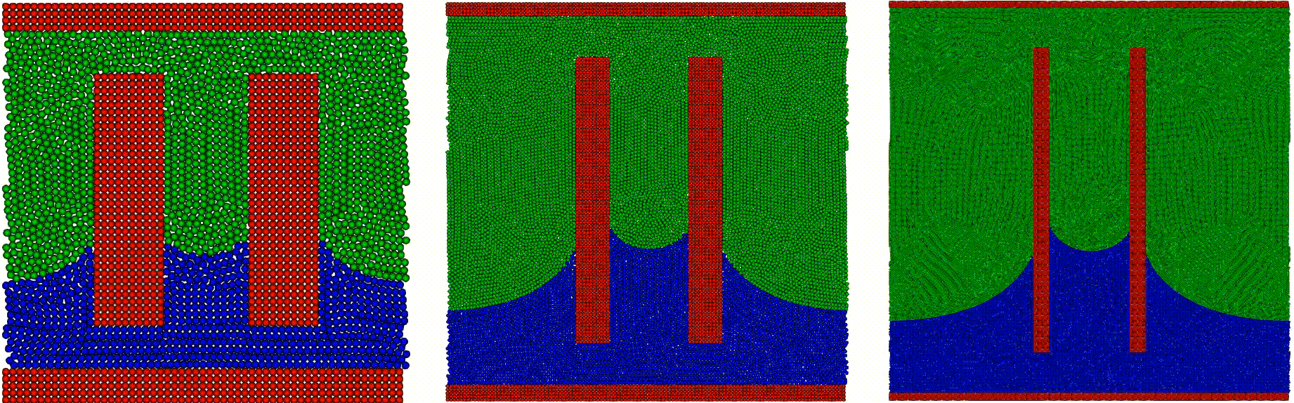
Figure 34: Steady state results with, from left to right, $60\times 60$, $140\times 140$ and $223\times 223$ particles for $\theta_{c}=30^{\circ}$

Figure 35: Measured error between the final height of the lower fluid for different resolutions and different contact angles

The lowest resolution is not able to correctly reproduce the fluid rise. Moreover, because of the low resolution, the thickness of the parallel plates is too important and does not properly represent the expected geometry. For the other resolutions, the error is between $5\%$ and $10\%$ showing the ability of the model to reproduce the expected behavior with a reasonable accuracy.

A.5 Rayleigh-Taylor Instability

The Rayleigh-Taylor instability is a famous two-phase instability where a heavy fluid is place on top of a light fluid with a given interface shape and submitted to gravity. Several SPH researchers have reproduced this case with SPH [22, 55]. The test case and its parameters are borrowed from [22]. The computational domain is twice as high as long, $H\times L$ with $H=2L$ and populated with $40000$ particles. The density ratio is $1.8$ while the viscosity ratio is $1$. Gravity is set $g=9.81\leavevmode\nobreak\ \mathrm{m}\mathrm{/}\mathrm{s}^{-2}$ and oriented downwards. Therefore, the viscosity $\nu$ is adjusted to math the desired Reynolds number $Re=\sqrt{\frac{(H/2)^{3}g}{\nu}}=420$. $\gamma=7.0$ for both fluids. No surface tension is used. No slip boundary conditions are applied at the walls. The interface is initialized as follows : $y=1-\sin(2\pi x)$. Time $t$ is nondimensionalized by $t_{g}=1/\sqrt{g/H}$.

The distribution of the two phases is shown at selected timesteps on Figure 36 superposed with results from [22]. In order to validate the model in a more quantitative way than just looking at the shape of the interface, vorticity has been calculated and is displayed on Figure 37a at selected timesteps. These vorticity plots can be compared with results presented on Figures 5 and 6 in [22] (and reproduced here on Figures 37b and 37c with permission) showing good agreement. Note that the SPH results from [22] where done with $180000$ particles.

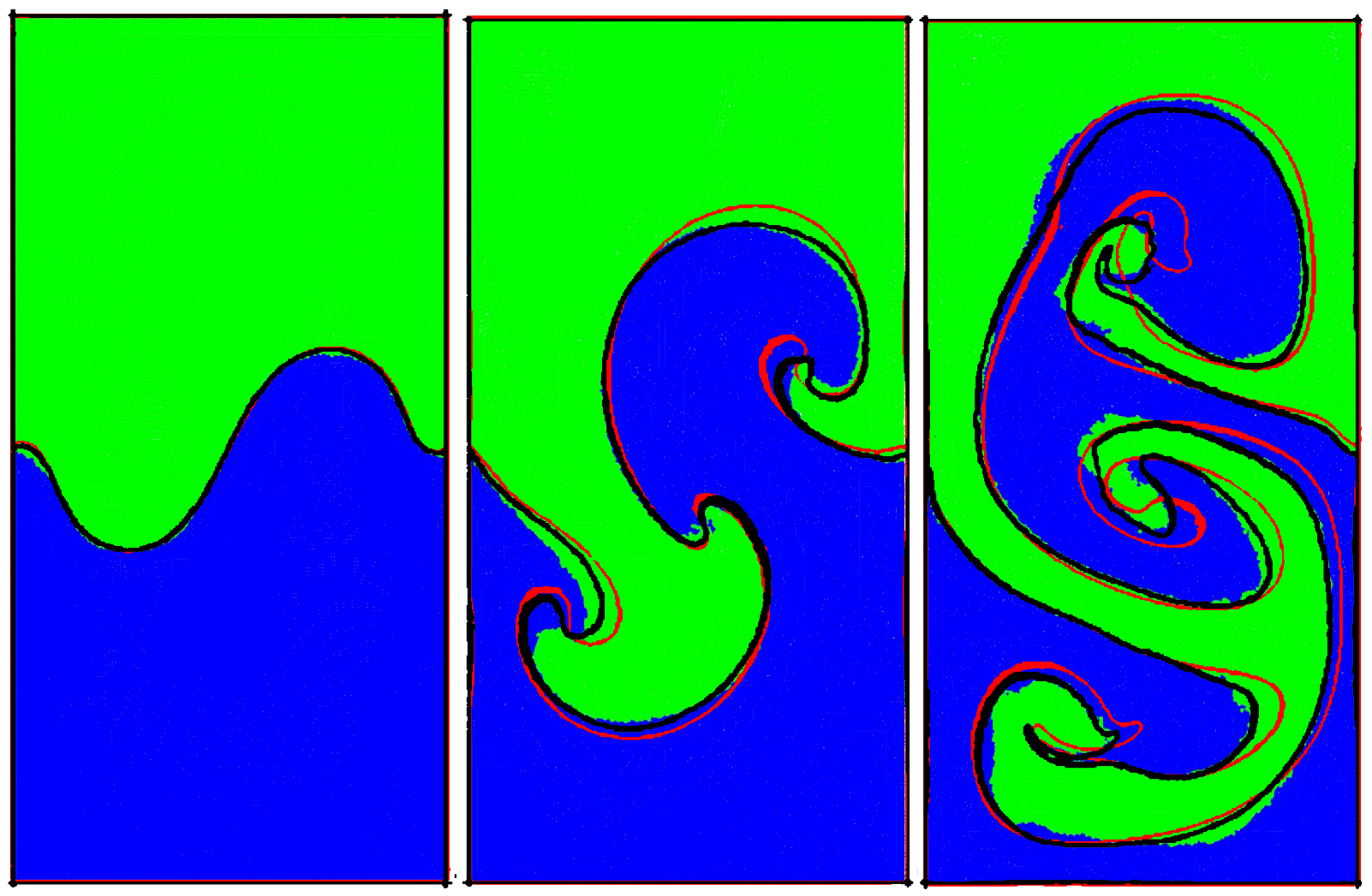
Figure 36: SPH phases distribution of Rayleigh-Taylor instability at selected timesteps : $t/t_{g}=1$, $3$ and $5$. Superposed with SPH interface (in black) and with Level-Set interface (in red) both extracted from [22]

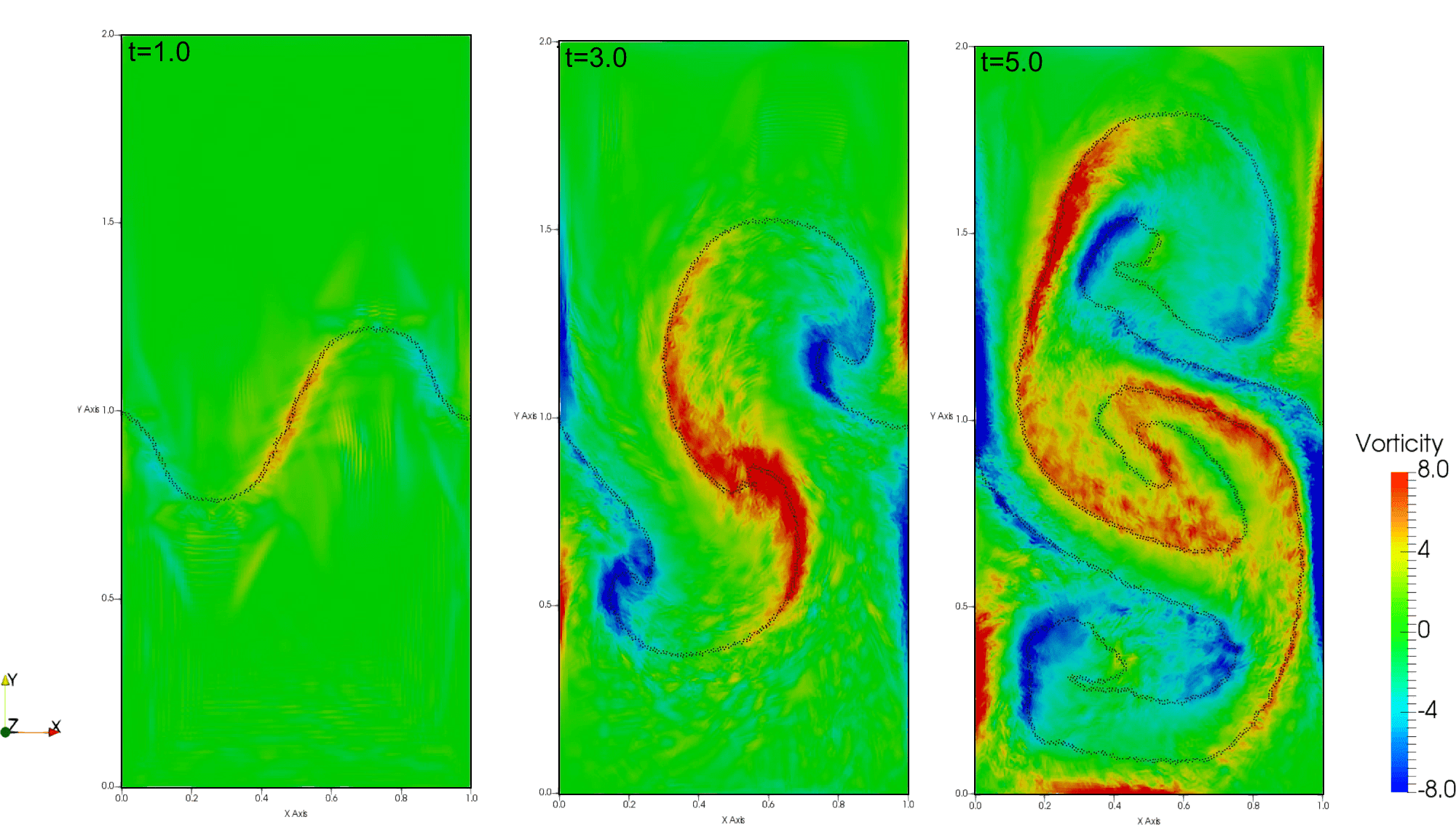
(a) Current work

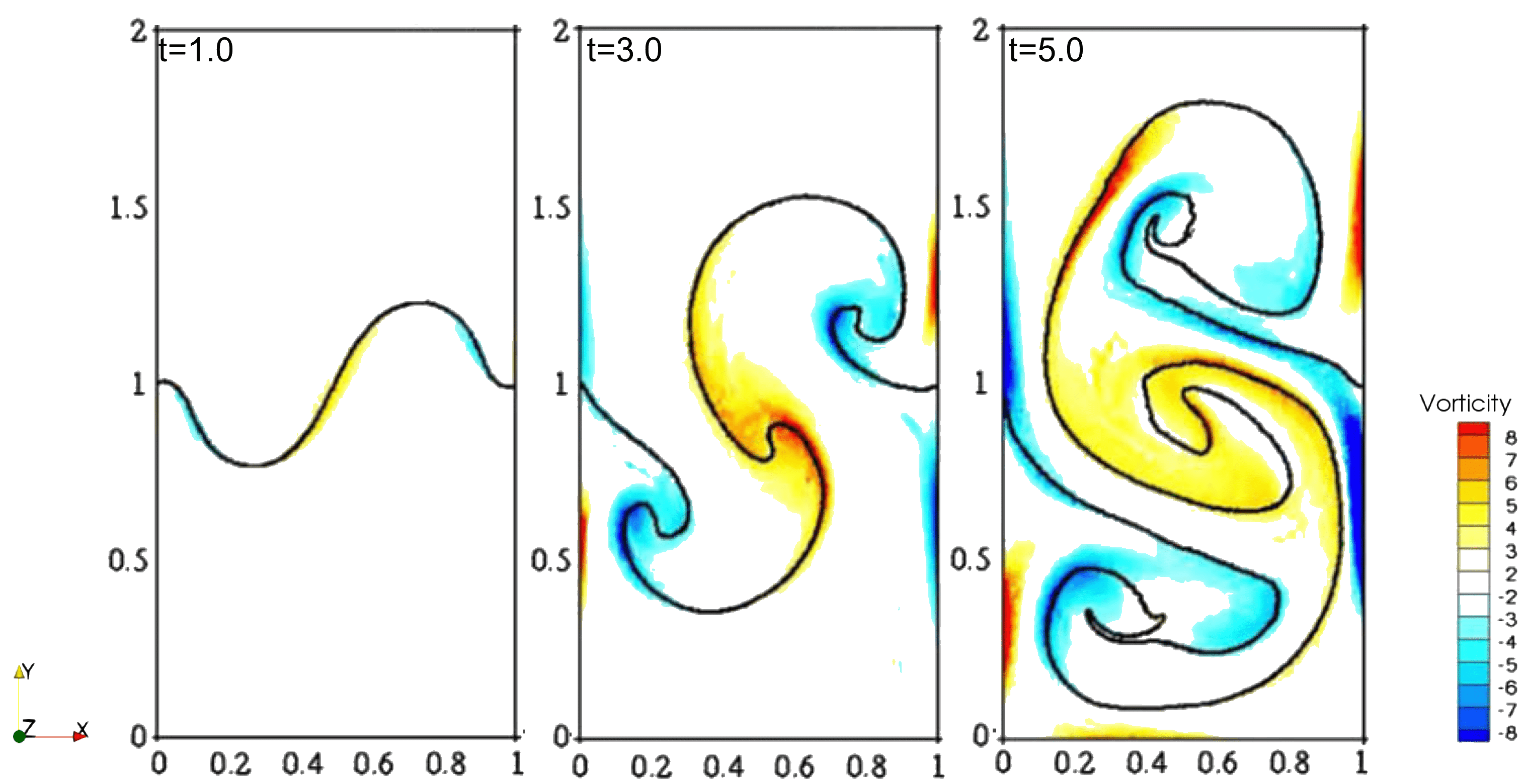
(b) SPH (from [22])

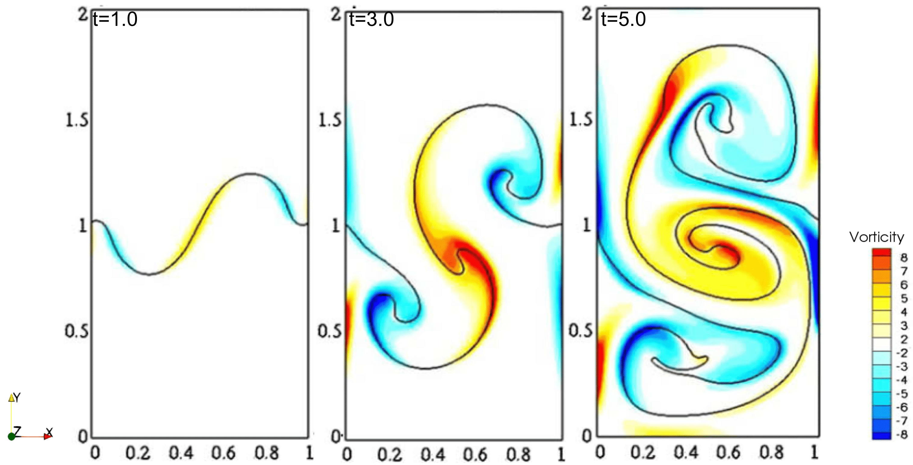
(c) Level Set (from [22])

Figure 37: Vorticity results of Rayleigh-Taylor instability at selected timesteps : $t/t_{g}=1$, $3$ and $5$

References

- [1] Z. I. Al-Hashimy, H. H. Al-Kayiem, R. W. Time, and Z. K. Kadhim. Numerical characterisation of slug flow in horizontal air/water pipe flow. International Journal of Computational Methods and Experimental Measurements, 4(2):114–130, 2016.
- [2] C. E. Alvarado-Rodríguez, J. Klapp, L. D. G. Sigalotti, J. M. Domínguez, and E. de la Cruz Sánchez. Nonreflecting outlet boundary conditions for incompressible flows using sph. Computers & Fluids, 159:177 – 188, 2017.
- [3] O. Baker. Design of pipelines for the simultaneous flow of oil and gas. In Fall Meeting of the Petroleum Branch of AIME. Society of Petroleum Engineers, 1953.
- [4] D. Barnea. A unified model for predicting flow-pattern transitions for the whole range of pipe inclinations. International Journal of Multiphase Flow, 13(1):1–12, jan 1987.
- [5] R. Belt, E. Duret, D. Larrey, B. Djoric, and S. Kalali. Comparison of commercial multiphase flow simulators with experimental and field databases. In 15th International Conference on Multiphase Production Technology, Cannes, France, 2011. BHR Group.
- [6] K. H. Bendiksen, D. Maines, R. Moe, and S. Nuland. The dynamic two-fluid model olga: Theory and application. SPE, 1991.
- [7] J. Bonet and T.-S. Lok. Variational and momentum preservation aspects of smooth particle hydrodynamic formulations. Computer Methods in Applied Mechanics and Engineering, 180(1):97 – 115, 1999.
- [8] J. Brackbill, D. Kothe, and C. Zemach. A continuum method for modeling surface tension. Journal of Computational Physics, 100(2):335 – 354, 1992.
- [9] A. Colagrossi and M. Landrini. Numerical simulation of interfacial flows by smoothed particle hydrodynamics. Journal of Computational Physics, 191(2):448 – 475, 2003.
- [10] W. Dehnen and H. Aly. Improving convergence in smoothed particle hydrodynamics simulations without pairing instability. Monthly Notices of the Royal Astronomical Society, 425(2):1068–1082, 2012.
- [11] S. Dong, G. Karniadakis, and C. Chryssostomidis. A robust and accurate outflow boundary condition for incompressible flow simulations on severely-truncated unbounded domains. Journal of Computational Physics, 261:83 – 105, 2014.
- [12] T. Douillet-Grellier, F. D. Vuyst, H. Calandra, and P. Ricoux. Influence of the spurious interface fragmentation correction on the simulation of flow regimes. In Proceedings of the International 13th SPHERIC Workshop, June 26-28, Galway, Ireland, 2018.
- [13] J. Fabre and A. Line. Modeling of two-phase slug flow. Annual Review of Fluid Mechanics, 24(1):21–46, jan 1992.
- [14] M. Ferrand, A. Joly, C. Kassiotis, D. Violeau, A. Leroy, F.-X. Morel, and B. D. Rogers. Unsteady open boundaries for sph using semi-analytical conditions and riemann solver in 2d. Computer Physics Communications, 210:29 – 44, 2017.
- [15] M. Ferrand, D. R. Laurence, B. D. Rogers, D. Violeau, and C. Kassiotis. Unified semi-analytical wall boundary conditions for inviscid, laminar or turbulent flows in the meshless SPH method. International Journal for Numerical Methods in Fluids, 71(4):446–472, mar 2012.
- [16] E. G. Flekkoy, P. V. Coveney, and G. De Fabritiis. Foundations of dissipative particle dynamics. Phys. Rev. E, 62:2140–2157, Aug 2000.
- [17] L. Friedel. Improved friction pressure drop correlations for horizontal and vertical two-phase pipe flow. In European Two-Phase Flow Group Meeting, Ispra, Italy. European Two-Phase Flow Group, 1979.
- [18] K. Fukagata, N. Kasagi, P. Ua-arayaporn, and T. Himeno. Numerical simulation of gas–liquid two-phase flow and convective heat transfer in a micro tube. International Journal of Heat and Fluid Flow, 28(1):72–82, feb 2007.
- [19] A. Ghaitanellis. Modélisation du charriage sédimentaire par une approche granulaire avec SPH. PhD thesis, Université Paris-Est, 2017. Thèse de doctorat dirigée par Violeau, Damien Mécanique des fluides Paris Est 2017.
- [20] U. Ghia, K. Ghia, and C. Shin. High-re solutions for incompressible flow using the navier-stokes equations and a multigrid method. Journal of Computational Physics, 48(3):387 – 411, 1982.
- [21] R. Gingold and J. Monaghan. Smoothed particle hydrodynamics-theory and application to non-spherical stars. Monthly Notices of the Royal Astronomical Society, 181:375–389, 1977.
- [22] N. Grenier, M. Antuono, A. Colagrossi, D. L. Touzé, and B. Alessandrini. An hamiltonian interface sph formulation for multi-fluid and free surface flows. Journal of Computational Physics, 228(22):8380 – 8393, 2009.
- [23] I. Hammani, G. Oger, D. L. Touzé, A. Colagrossi, and S. Marrone. How to derive the multi-fluid delta-sph model. In Proceedings of the International 13th SPHERIC Workshop, June 26-28, Galway, Ireland, 2018.
- [24] Q. He and N. Kasagi. Phase-field simulation of small capillary-number two-phase flow in a microtube. Fluid Dynamics Research, 40(7-8):497–509, jul 2008.
- [25] G. F. Hewitt. Two-Phase Flows. In A-to-Z Guide to Thermodynamics, Heat and Mass Transfer, and Fluids Engineering. Begellhouse.
- [26] X. Hu and N. Adams. A multi-phase SPH method for macroscopic and mesoscopic flows. Journal of Computational Physics, 213(2):844 – 861, 2006.
- [27] X. Hu and N. Adams. An incompressible multi-phase sph method. Journal of Computational Physics, 227(1):264 – 278, 2007.
- [28] S. Khorasanizade and J. M. M. Sousa. An innovative open boundary treatment for incompressible sph. International Journal for Numerical Methods in Fluids, 80(3):161–180, 2016. FLD-14-0455.R2.
- [29] Kongsberg. LedaFlow - The new multiphase simulator: User guide. Kongsberg, 2014.
- [30] P. Kunz, M. Hirschler, M. Huber, and U. Nieken. Inflow/outflow with dirichlet boundary conditions for pressure in isph. Journal of Computational Physics, 326:171 – 187, 2016.
- [31] P. Kunz, I. M. Zarikos, N. K. Karadimitriou, M. Huber, U. Nieken, and S. M. Hassanizadeh. Study of multi-phase flow in porous media: Comparison of SPH simulations with micro-model experiments. Transport in Porous Media, 114(2):581–600, nov 2015.
- [32] B. Lafaurie, C. Nardone, R. Scardovelli, S. Zaleski, and G. Zanetti. Modelling merging and fragmentation in multiphase flows with surfer. Journal of Computational Physics, 113(1):134 – 147, 1994.
- [33] M. Lastiwka, M. Basa, and N. J. Quinlan. Permeable and non-reflecting boundary conditions in SPH. International Journal for Numerical Methods in Fluids, 61(7):709–724, 2009.
- [34] A. Leroy, D. Violeau, M. Ferrand, and C. Kassiotis. Unified semi-analytical wall boundary conditions applied to 2-d incompressible SPH. Journal of Computational Physics, 261:106–129, mar 2014.
- [35] L. Libersky, A. Petschek, T. Carney, J. Hipp, and F. Allahdadi. High strain lagrangian hydrodynamics:: A three-dimensional SPH code for dynamic material response. Journal of Computational Physics, 109(1):67–75, 1993.
- [36] E. Lizarraga-García. A study of Taylor bubbles in vertical and inclined slug flow using multiphase CFD with level set. PhD thesis, Massachusetts Institute of Technology, 2016.
- [37] R. W. Lockhart and R. C. Martinelli. Proposed correlation of data for isothermal two-phase, two-component flow in pipes. Chemical Engineering Progress, 45(1):39–48, 1949.
- [38] M. Lu. Experimental and computational study of two-phase slug flow. PhD thesis, Imperial College London, 2015.
- [39] J.-P. Minier. Simulation of two-phase flow patterns with a new approach based on smoothed particle hydrodynamics. NUGENIA Project SPH-2PHASEFLOW Presentation Slides, 2016.
- [40] A. Mokos, B. D. Rogers, and P. K. Stansby. A multi-phase particle shifting algorithm for SPH simulations of violent hydrodynamics with a large number of particles. Journal of Hydraulic Research, 55(2):143–162, sep 2016.
- [41] J. Monaghan. Smoothed particle hydrodynamics. Annu, Rev, Astron. Astrophys., 30:543–74, 1992.
- [42] J. Monaghan. A turbulence model for smoothed particle hydrodynamics. European Journal of Mechanics - B/Fluids, 30(4):360–370, jul 2011.
- [43] J. J. Monaghan. Smoothed particle hydrodynamics. Reports on Progress in Physics, 68(8):1703, 2005.
- [44] J. Morris, P. Fox, and Y. Zhu. Modeling low reynolds number incompressible flows using SPH. Journal of Computational Physics, 136(1):214–226, 1997.
- [45] J. P. Morris. Simulating surface tension with smoothed particle hydrodynamics. International Journal for Numerical Methods in Fluids, 33(3):333–353, 2000.
- [46] H. Müller-Steinhagen and K. Heck. A simple friction pressure drop correlation for two-phase flow in pipes. Chemical Engineering and Processing: Process Intensification, 20(6):297–308, nov 1986.
- [47] G. Oger, M. Doring, B. Alessandrini, and P. Ferrant. Two-dimensional sph simulations of wedge water entries. Journal of Computational Physics, 213(2):803 – 822, 2006.
- [48] S. Pedersen, P. Durdevic, and Z. Yang. Challenges in slug modeling and control for offshore oil and gas productions: A review study. International Journal of Multiphase Flow, 88:270 – 284, 2017.
- [49] B. D. Rogers and R. A. Dalrymple. SPH modeling of tsunami waves. In Advances in Coastal and Ocean Engineering, pages 75–100. World Scientific, sep 2008.
- [50] F. Sánchez-Silva, I. Carvajal-Mariscal, M. Toledo-Velázquez, D. Libreros, M. Toledo-Velázquez, and H. Saidani-Scott. Experiments in a combined up stream downstream slug flow. EPJ Web of Conferences, 45:01082, 2013.
- [51] C. Sarica and O. Shoham. A simplified transient model for pipeline-riser systems. Chemical Engineering Science, 46(9):2167 – 2179, 1991.
- [52] A. Sausen, P. Sausen, and M. de. The slug flow problem in oil industry and pi level control. In New Technologies in the Oil and Gas Industry. InTech, oct 2012.
- [53] S. Shao and H. Gotoh. Turbulence particle models for tracking free surfaces. Journal of Hydraulic Research, 43(3):276–289, may 2005.
- [54] P. Spedding, E. Benard, and G. Donnelly. Prediction of pressure drop in multiphase horizontal pipe flow. International Communications in Heat and Mass Transfer, 33(9):1053–1062, nov 2006.
- [55] K. Szewc. Développement d’une approche particulaire de type SPH pour la modélisation des écoulements multiphasiques avec interfaces variables. PhD thesis, Université de Lorraine, jun 2013.
- [56] K. Szewc and M. T. Lewandowski. Further investigation of the spurious interface fragmentation in multiphase smoothed particle hydrodynamics, 2016.
- [57] K. Szewc, K. Walczewska-Szewc, and M. Olejnik. Is the motion of a single sph particle droplet/solid physically correct?, 2016.
- [58] A. Tafuni, J. Domínguez, R. Vacondio, and A. Crespo. A versatile algorithm for the treatment of open boundary conditions in smoothed particle hydrodynamics gpu models. Computer Methods in Applied Mechanics and Engineering, 2018.
- [59] T. Taha and Z. Cui. Hydrodynamics of slug flow inside capillaries. Chemical Engineering Science, 59(6):1181–1190, mar 2004.
- [60] Y. Taitel, D. Bornea, and A. E. Dukler. Modelling flow pattern transitions for steady upward gas-liquid flow in vertical tubes. AIChE Journal, 26(3):345–354, 1980.
- [61] Y. Taitel and A. E. Dukler. A model for predicting flow regime transitions in horizontal and near horizontal gas-liquid flow. AIChE Journal, 22(1):47–55, jan 1976.
- [62] A. M. Tartakovsky and A. Panchenko. Pairwise force smoothed particle hydrodynamics model for multiphase flow: Surface tension and contact line dynamics. Journal of Computational Physics, 305:1119 – 1146, 2016.
- [63] A. M. Tartakovsky, N. Trask, K. Pan, B. Jones, W. Pan, and J. R. Williams. Smoothed particle hydrodynamics and its applications for multiphase flow and reactive transport in porous media. Computational Geosciences, pages 1–28, 2015.
- [64] N. Tofighi and M. Yildiz. Numerical simulation of single droplet dynamics in three-phase flows using isph. Computers & Mathematics with Applications, 66(4):525 – 536, 2013.
- [65] K. Triplett, S. Ghiaasiaan, S. Abdel-Khalik, and D. Sadowski. Gas–liquid two-phase flow in microchannels part i: two-phase flow patterns. International Journal of Multiphase Flow, 25(3):377–394, apr 1999.
- [66] M. Viggiani, O. Mariani, V. Battarra, A. Annunziato, and U. Bollettini. A model to verify the onset of severe slugging. In PSIG Annual Meeting, Toronto, Ontario, 1988. Pipeline Simulation Interest Group.
- [67] D. Violeau and R. Issa. Numerical modelling of complex turbulent free-surface flows with the SPH method: an overview. International Journal for Numerical Methods in Fluids, 53(2):277–304, 2006.
- [68] D. Violeau and A. Leroy. On the maximum time step in weakly compressible SPH. Journal of Computational Physics, 256:388 – 415, 2014.
- [69] M. Wambsganss, J. Jendrzejczyk, and D. France. Two-phase flow and pressure drop in flow passages of compact heat exchangers. Technical report, Argonne National Lab., IL (United States), 1992.
- [70] Z.-B. Wang, R. Chen, H. Wang, Q. Liao, X. Zhu, and S.-Z. Li. An overview of smoothed particle hydrodynamics for simulating multiphase flow. Applied Mathematical Modelling, 40(23-24):9625–9655, dec 2016.
- [71] H. Wendland. Piecewise polynomial, positive definite and compactly supported radial functions of minimal degree. Advances in Computational Mathematics, 4(1):389–396, Dec 1995.
- [72] F. Xie, X. Zheng, M. S. Triantafyllou, Y. Constantinides, Y. Zheng, and G. Em Karniadakis. Direct numerical simulations of two-phase flow in an inclined pipe. Journal of Fluid Mechanics, 825:189?207, 2017.
- [73] C. Yao, Y. Liu, C. Xu, S. Zhao, and G. Chen. Formation of liquid-liquid slug flow in a microfluidic t-junction: Effects of fluid properties and leakage flow. AIChE Journal, 64(1):346–357, aug 2017.
- [74] M. Yildiz, R. A. Rook, and A. Suleman. SPH with the multiple boundary tangent method. International Journal for Numerical Methods in Engineering, 77(10):1416–1438, mar 2009.
- [75] Z. Yu, O. Hemminger, and L.-S. Fan. Experiment and lattice boltzmann simulation of two-phase gas–liquid flows in microchannels. Chemical Engineering Science, 62(24):7172–7183, dec 2007.
- [76] A. Zainali, N. Tofighi, M. Shadloo, and M. Yildiz. Numerical investigation of newtonian and non-newtonian multiphase flows using isph method. Computer Methods in Applied Mechanics and Engineering, 254:99 – 113, 2013.
- [77] M. Zhang, L. ming Pan, P. Ju, X. Yang, and M. Ishii. The mechanism of bubbly to slug flow regime transition in air-water two phase flow: A new transition criterion. International Journal of Heat and Mass Transfer, 108:1579 – 1590, 2017.