Suppression of Quantum-Mechanical Collapse in Bosonic Gases with Intrinsic Repulsion: a Brief Review

Abstract

It is known that attractive potential $\sim-1/r^{2}$ gives rise to the critical quantum collapse in the framework of the three-dimensional (3D) linear Schrödinger equation. This article summarizes theoretical analysis, chiefly published in several original papers, which demonstrates suppression of the collapse caused by this potential, and the creation of the otherwise missing ground state in a 3D gas of bosonic dipoles pulled by the same potential to the central charge, with repulsive contact interactions between them, represented by the cubic term in the respective Gross-Pitaevskii equation (GPE). In two dimensions (2D), quintic self-repulsion is necessary for the suppression of the collapse; alternatively, this may be provided by the effective quartic repulsion, produced by the Lee-Huang-Yang correction to the GPE. 3D states carrying angular momentum are constructed in the model with the symmetry reduced from spherical to cylindrical by an external polarizing field. Interplay of the collapse suppression and miscibility-immiscibility transition is considered in a binary condensate. The consideration of the 3D setting in the form of the many-body quantum system, with the help of the Monte Carlo method, demonstrates that, although the quantum collapse cannot be fully suppressed, the self-trapped states, predicted by the GPE, exist in the many-body setting as metastable modes protected against the collapse by a tall potential barrier.

quantum anomaly; ground state; self-trapping; Bose-Einstein condensate; Gross-Pitaevskii equation; Thomas-Fermi approximation; mean-field approximation; quantum phase transitions; Monte Carlo method

Abbreviations

2D	two-dimensional
3D	three-dimensional
BEC	Bose-Einstein condensate
GPE	Gross-Pitaevskii equation
LHY	Lee-Huang-Yang (correction to the mean-field theory)
GS	ground state
rms	root-mean-square (value)
TFA	Thomas-Fermi approximation

I Introduction

One of standard exercises given to students taking the course of quantum mechanics is solving the three-dimensional (3D) Schrödinger equation with an isotropic attractive potential,

$$U(r)=-\frac{U_{0}}{2r^{2}},~{}U_{0}>0$$ (1)

LL . This exercise offers a unique example of critical phenomena in the nonrelativistic quantum theory. Indeed, the corresponding classical (Newton’s) equation of motion for the particle’s coordinates, $\mathbf{r}=\left\{x,y,z\right\}$,

$$\frac{d^{2}\mathbf{r}}{dt^{2}}=-\frac{\partial U}{\partial\mathbf{r}}\equiv U_{0}\frac{\mathbf{r}}{r^{4}},$$ (2)

admits obvious rescaling, $t\equiv\tilde{t}/\sqrt{U_{0}}$, which eliminates $U_{0}$ from Eq. (2), thus making the solution invariant with respect to the choice of a positive value of the potential strength, $U_{0}$. However, the invariance is lost in the corresponding 3D Schrödinger equation for wave function $\psi\left(\mathbf{r},t\right)$,

$$i\psi_{t}=-\frac{1}{2}\nabla^{2}\psi-\frac{U_{0}}{2r^{2}}\psi,$$ (3)

in which $U_{0}$ cannot be removed by rescaling. This drastic difference between the classical mechanical system and its quantum-mechanical counterpart is known as the quantum anomaly , alias “dimensional transmutation” anomaly ; anomaly2 . The consequence of the anomaly is well known: if an external trapping potential,

$$U_{\mathrm{trap}}=\frac{1}{2}\Omega^{2}r^{2},$$ (4)

is added to Eq. (3), to make the integral norm,

$$N=\int\left|\psi(\mathbf{r})\right|^{2}d\mathbf{r,}$$ (5)

convergent at $r\rightarrow\infty$, the Schrödinger equation gives rise to the normal set of trapped modes, starting from the ground state (GS), at

$$U_{0}<\left(U_{0}\right)_{\mathrm{cr}}^{(\mathrm{3D})}=1/4.$$ (6)

On the other hand, above this critical point, i.e., at $U_{0}>1/4$, the GS does not exist (or, formally, speaking, it has an infinitely small size, corresponding to energy $E\rightarrow-\infty$, which is known as “fall onto the center” LL , the other name for which is “quantum collapse” anomaly ; anomaly2 ).

In the 2D space, the quantum collapse, driven by the same potential (1), is more violent, taking place at any value $U_{0}>0$ (in other words, the respective critical value is $\left(U_{0}\right)_{\mathrm{cr}}^{\mathrm{(2D)}}=0$). Finally, in the 1D case the same potential (1) gives rise to a still stronger superselection effect, which means splitting the 1D space into two non-communicating subspaces, $x\gtrless 0$ superselection .

A solution to the quantum-collapse problem in the 3D case was proposed in terms of a linear quantum-field-theory, replacing the usual quantum-mechanical wave function by the secondary-quantized field anomaly ; anomaly2 . This approach makes it possible to introduce the GS, which is missing at $U_{0}>1/4$ in the framework of standard quantum mechanics. However, the solution does not predict a definite value of the size of the newly created GS. Instead, the field-theory formulation, based on the renormalization-group technique, introduces a GS with an arbitrary spatial scale, in terms of which all other spatial sizes are measured in that setting.

The present mini-review aims to summarize results produced by works which elaborated another possibility to resolve the problem of the quantum collapse. This possibility was proposed in Ref. HS1 , and then developed, for more general situations, in works HS2 and HS3 . The solution was based on the consideration of an ultracold gas of bosonic particles pulled to the center by potential (1). The gas was assumed to be in the state of the Bose-Einstein condensate (BEC) BEC , and the suppression of the single-particle quantum collapse in this coherent many-body setting was provided by repulsive contact interactions between colliding particles in the gas. The solution was elaborated in the framework of the mean-field approach BEC , i.e., treating the single-particle wave function, which represents all particles in the gas, as a classical field governed by the corresponding Gross-Pitaevskii equation (GPE).

The same work HS1 offered a physical realization of potential (1) in the 3D space, which was previously considered as a formal exercise LL . The realization is provided by assuming that the bosonic particles are small molecules carrying a permanent electric dipole moment, $d$, pulled by the electrostatic force to a point-like charge, $Q$, placed at the origin, which creates electric field $\mathbf{E}=Q\mathbf{r}/r^{3}$. In this connection, it is relevant to mention that it has been demonstrated experimentally that a free charge (ion), immersed in an ultracold gas, may be kept at a fixed position by means of a laser-trapping technique ion . Assuming that the orientation of the dipole carried by each particle is locked to the local field, i.e., $\mathbf{d/}d=\mathrm{sgn}(Q)\left(\mathbf{r}/r\right)$, so as to minimize the interaction energy, the respective interaction potential is $U(r)=-\mathbf{d}\cdot\mathbf{E}$, which is tantamount to potential (1) with strength

$$U_{0}=2|Q|d.$$ (7)

As for the dipolar molecules which may be used to build the BEC under the consideration, experimental results suggest that they may be, e.g., LiCs LiCs or KRb KRb .

The gas of ultracold dipolar molecules, trapped in a pancake-shaped configuration shaped by an appropriate external potential 2D-review , with the central electric charge immersed in the gas as outlined above, provides for the realization of the 2D version of the setting. An alternative realization of the 2D setting is offered by a gas of polarizable atoms without a permanent dielectric moment, while an effective moment is induced in them by the electric field of a uniformly charged wire set perpendicular to the pancake’s plane Schmiedmayer , or with an effective magnetic moment induced by a current filament (e.g., an electron beam) piercing the pancake perpendicularly.

In the context of 2D settings, it is relevant to mention that a quantum anomaly was also predicted in a model described by the GPE in the 2D space, for a gas of bosons with the repulsive contact interaction, trapped in the harmonic-oscillator potential (4) Olshanii . The anomaly breaks the specific scaling invariance of this gas, which holds in the mean-field approximation.

In terms of the GPE, the contact repulsive interaction in the bosonic gas is represented by the cubic term BEC . With the addition of this term, and taking into regard the external trapping potential (4), which is present in any experiment with ultracold atoms, the linear Schrödinger equation (3) is replaced by the GPE, which is written here in the scaled form:

$$i\psi_{t}=-\frac{1}{2}\left(\nabla^{2}+\frac{U_{0}}{r^{2}}-\Omega^{2}r^{2}\right)\psi+\left|\psi\right|^{2}\psi.$$ (8)

It is relevant to mention that the 3D GPE with the self-attractive interaction, which corresponds to the opposite sign in front of the cubic term in Eq. (8), gives rise, in the absence of the attractive potential ($U_{0}=0$) to the well-known supercritical wave collapse Berge' . A relation of this setting to Eq. (8) is that the inclusion of the trapping potential $\sim\Omega^{2}$ gives rise to stable bound states in the form of spherically symmetric bound states and ones with vorticity $m=1$ (cf. Eq. (16) below), provided that norm $N$ does not exceed a certain critical value Dodd -DumDum .

The energy (Hamiltonian) corresponding to Eq. (8) is

$$E=\frac{1}{2}\int\left[\left|\nabla\psi\right|^{2}-\left(\frac{U_{0}}{r^{2}}-\Omega^{2}r^{2}\right)\left|\psi\right|^{2}+\left|\psi^{4}\right|\right]d\mathbf{r},$$ (9)

The scaled variables and constants, in terms of which Eq. (8) is written, are related to their counterparts measured in physical units:

$$\mathbf{r}=\frac{\mathbf{r}_{\mathrm{ph}}}{r_{0}},~{}t=\frac{\hbar}{mr_{0}^{2}}t_{\mathrm{ph}},~{}~{}\psi=2\sqrt{\pi a_{s}}r_{0}\psi_{\mathrm{ph}},~{}U_{0}=\frac{m}{\hbar^{2}}\left(U_{0}\right)_{\mathrm{ph}},~{}\Omega=\frac{mr_{0}^{2}}{\hbar}\Omega_{\mathrm{ph}},$$ (10)

where $m$ and $a_{s}$ are the bosonic mass and s-scattering length, which accounts for the repulsive interactions between the particles BEC , and $r_{0}$ is an arbitrary spatial scale. The total number of bosons in the gas is given by

$$N_{\mathrm{ph}}=\int\left|\psi_{\mathrm{ph}}(\mathbf{r}_{\mathrm{ph}})\right|^{2}d\mathbf{r}_{\mathrm{ph}}\equiv\frac{r_{0}N}{4\pi a_{s}},$$ (11)

where the norm of the scaled wave function is given by Eq. (5).

It is relevant to note that, as it follows from Eq. (7) and rescaling (10), the above-mentioned critical value, $U_{0}=1/4$, of the strength of the attractive potential (see Eq. (6)) corresponds to a very small dipole moment, $d\sim 10^{-6}$ Debye, if central charge $Q$ is taken as the elementary charge, and the mass of the particle is $\sim 100$ proton masses. Therefore, the overcritical case of $U_{0}>1/4$, the consideration of which is the main objective of the present article, is relevant in the actual physical context.

Taken as Eq. (8), the GPE neglects dipole-dipole interactions between the particles. These interactions can be taken into account in the framework of another application of the mean-field approach. Indeed, the local density of the dipole moment in the gas (i.e., the dielectric polarization of the medium) is $\mathbf{P}=\mathbf{d}\left|\psi(\mathbf{r})\right|^{2}$, hence the electrostatic field generated by the polarization, $\mathbf{E}_{d}$, is determined by the Poisson equation, $\nabla\cdot\left(\mathbf{E}_{d}+4\pi\mathbf{P}\right)=0$, which can be solved immediately:

$$\mathbf{E}_{d}=-4\pi\mathbf{P}\equiv-4\pi\mathbf{d}\left|\psi(\mathbf{r})\right|^{2}.$$ (12)

Then, the extra term in the GPE, accounting for the interaction of the local dipole with the collective field (12), created by all the other dipoles, is

$$-\left(\mathbf{d}\cdot\mathbf{E}_{d}\right)\psi\equiv 4\pi d^{2}\left|\psi\right|^{2}\psi.$$ (13)

This term, if added to Eq. (8), may be absorbed into a redefinition of the scattering length accounting for the repulsion between the particles. In the underlying physical units, this amounts to

$$a_{s}\rightarrow\left(a_{s}\right)_{\mathrm{eff}}\equiv a_{s}+md^{2}/\hbar^{2},$$ (14)

where $m$ is the mass of the dipolar molecule. For the typical value of $a_{s}\sim 10$ nm and the above-mentioned mass of the particle, $\sim 100$ proton masses, Eq. (14) demonstrates that the additional term is essential for dipole moments $d\gtrsim 0.3$ Debye.

The rest of the article is organized as follows. In Section II, results are reported for the basic model, outlined above, as per Ref. HS1 . Particular subsections of Section II first recapitulate the description of the 3D and 2D collapse in the framework of Schrödinger equation (3), which includes the trapping potential (4), and then present main results obtained in the 3D case on the basis of Eq. (8) (with $\Omega=0$, as the trapping potential is not a necessary ingredient of the nonlinear model, on the contrary to the linear one). The results explicitly demonstrate the creation of the originally missing GS by the self-repulsive cubic nonlinearity at $U_{0}>1/4$. In addition, a subsection of Section II reports a new result, viz., a quantum phase transition in the GS of the model which includes the Lee-Huang-Yang (LHY) correction LHY to the mean-field GPE. The summary of results for the 2D nonlinear model are also presented in Section II. It is demonstrated that the cubic self-repulsive term is insufficient for the suppression of the 2D quantum collapse and restoration of the missing GS. This is possible if a quintic repulsive term is included in the GPE, which may account for three- body collisions, or if the quartic LHY correction is included in the effective two-dimensional GPE . A short subsection concluding Section II formulates a challenging problem of the consideration of the quantum collapse in the gas of fermions.

Section III addresses, along the lines of Ref. HS2 , the collapse suppression and creation of the GS in the 3D model with the symmetry of the effective attractive potential reduced from spherical to cylindrical by an external field which polarizes dipole moments of the particles. In this version of the model, states carrying the angular momentum are constructed too, in addition to the GS.

Section IV deals with a two-component model in 3D, which makes it possible to consider the interplay of the collapse suppression and the transition between miscibility and immiscibility in the binary system. A weak quantum phase transition, which occurs in that setting, is also briefly considered in Section IV.

Section V presents results for the basic 3D model, considered in terms of the many-body quantum theory, as per Ref. GEA , with the help of variational approximation for the many-body wave functions and numerically implemented Monte Carlo method. The main result is that, strictly speaking, the quantum collapse is not fully suppressed in the many-body theory, but, nevertheless, the noncollapsing self-trapped state, predicted by the mean-field theory, exists as a metastable one, insulated from the collapse by a tall potential barrier.

The paper is concluded by Section VI, which also suggests directions for further work on this general topic.

II The basic three- and two-dimensional models

This section summarizes results produced in Ref. HS1 . The quantum phase transition driven by the LHY correction to the mean-field theory, briefly outlined in subsection 3, is a new finding.

II.1 The quantum collapse in the linear Schrödinger equation

First, it is relevant to recapitulate the analysis of linear Schrödinger equation (3), to which the trapping potential (4) is added:

$$i\psi_{t}=-\frac{1}{2}\left(\nabla^{2}+\frac{U_{0}}{r^{2}}-\Omega^{2}r^{2}\right)\psi.$$ (15)

Stationary solutions of Eq. (15) in 3D spherical coordinates, $\left(r,\theta,\varphi\right)$, are looked for as

$$\psi_{\mathrm{3D}}=\exp(-i\mu t)Y_{lm}\left(\theta,\varphi\right)\Phi(r),$$ (16)

where $\mu$ is the energy eigenvalue (or chemical potential, in terms of the GPE), $Y_{lm}\left(\theta,\varphi\right)$ is the spherical harmonic with quantum numbers $\left(l,m\right)$, and radial wave function $\Phi(r)$ is real. Substituting ansatz (16) in Eq. (15), two exact solutions for $\Phi(r)$ can be found:

$$\Phi(r)=\Phi_{0}r^{-\sigma_{\pm}}\exp\left(-\Omega r^{2}/2\right),$$ (17)

$$\mu=\Omega\left(\frac{3}{2}-\sigma_{\pm}\right),~{}\sigma_{\pm}\equiv\frac{1}{2}\pm\sqrt{\frac{1}{4}-U_{l}},$$ (18)

which exist under condition

$$U_{l}\equiv U_{0}-l\left(l+1\right)<1/4.$$ (19)

The smaller value of $\mu$ (in the case of $l=0$, it defines the GS of the system under the consideration) corresponds to $\sigma_{+}$, i.e.,, the top sign in Eq. (18). The wave function is characterized by its norm (5),

$$N=4\pi\int_{0}^{\infty}\Phi^{2}(r)r^{2}dr=2\pi\Phi_{0}^{2}\Omega^{-\left(1\mp\sqrt{\frac{1}{4}-U_{l}}\right)}\Gamma\left(1\mp\sqrt{\frac{1}{4}-U_{l}}\right),$$ (20)

where $\Gamma$ is the Gamma-function. Equation (20) shows why the trapping potential $\sim\Omega^{2}$ is necessary for the existence of physically relevant (normalizable) eigenmodes of the linear Schrödinger equation (15), as norm (20) diverges (due to its weak localization at $r\rightarrow\infty$) in the limit of $\Omega\rightarrow 0$.

These solutions for the stationary wave functions do not exist at $U_{l}>1/4$ (note that the presence of the angular momentum, $l\geq 1$, secures the existence of the bound states at essentially larger values of $U_{0}$, as per Eq. (19)). The nonexistence of stationary wave functions implies that the system suffers the onset of the quantum collapse, as confirmed by simulations of time-dependent equation (15), see an example in Fig. 1. Indeed, a set of instantaneous profiles of $\sqrt{r}|\psi(r,t)|$, shown in Fig. 1 for the weakly overcritical case, $U_{0}=0.27$, with $l=0$, confirm the development of the self-compression (finally, collapse) of the wave function towards $r=0$ (in the simulations, the collapse is eventually arrested due to a finite mesh size of the numerical scheme).

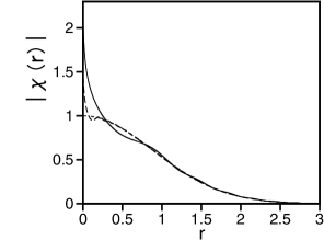
Figure 1: Radial profiles of $|\chi(r,t)|\equiv\sqrt{r}|\psi(r)|$ at $t=0$, $0.005$ and $0.1$ (dotted, dashed, and solid curves, respectively), as originally produced in Ref. HS1 by simulations of Eq. (15) with $\Omega^{2}=0.1$ and $U_{0}=0.27$, which slightly exceeds the critical one, $\left(U_{0}\right)_{\mathrm{cr}}^{\mathrm{(3D)}}=1/4$. The initial conditions is taken as $\psi_{0}(r)=r^{-1/2}\exp(-\Omega r^{2}/2)$, which is the exact stationary wave function for $U_{0}=1/4$, i.e., precisely at the critical point, taken as per Eqs. (17) and (18) (for this reason, the evolution of the wave function is displayed here in terms of $\sqrt{r}|\psi(r)|$). The simulations demonstrate the onset of the quantum collapse in the linear Schrödinger equation.

In 2D, the GS solution to Eq. (15) exists only for $U_{0}<0$. In the exact form, the GS wave function is given by Eqs. (16) and (17), but with (18) replaced by

$$\mu=\Omega\left(1-\sigma_{\pm}\right),\sigma_{\pm}=\pm\sqrt{-U_{0}}.$$ (21)

Direct simulations of the 2D equation (15) at $U_{0}>0$ also demonstrate the onset of the collapse dynamics.

II.2 The three-dimensional ground state (GS) created by the cubic self-repulsive nonlinearity

The most essential results may be produced by GPE (8) without an external trapping potential, hence the equation simplifies to

$$i\psi_{t}=-\frac{1}{2}\left(\nabla^{2}+\frac{U_{0}}{r^{2}}\right)\psi+\left|\psi\right|^{2}\psi.$$ (22)

The substitution of $\psi=e^{-i\mu t}\Phi(r)$ for isotropic stationary states of Eq. (22) (here, solely $l=0$ is considered, cf. Eq. (16), with the intention to construct the GS, which always has $l=0$) yields equation

$$\mu\Phi=-\frac{1}{2}\left(\frac{d^{2}\Phi}{dr^{2}}+\frac{2}{r}\frac{d\Phi}{dr}+\frac{U_{0}}{r^{2}}\right)\Phi+\Phi^{3}.$$ (23)

Scaling invariance of Eq. (23) at $r\rightarrow 0$ suggests that the respective asymptotic form of the solution should be $\Phi\sim 1/r$, therefore solutions are looked for as

$$\Phi\left(r\right)=\frac{\chi(r)}{r},$$ (24)

with function $\chi(r)$ obeying equation

$$\mu\chi=-\frac{1}{2}\left[\chi^{\prime\prime}+\left(\frac{U_{0}}{r^{2}}-\Omega^{2}r^{2}\right)\chi\right]+\frac{\chi^{3}}{r^{2}}.$$ (25)

Asymptotic forms of solutions to Eq. (25) can be readily constructed for $r\rightarrow 0$ and $r\rightarrow\infty$. First, the expansion at $r\rightarrow 0$ yields

$$\chi(r)=\sqrt{U_{0}/2}+\chi_{1}r^{s/2},~{}s\equiv 1+\sqrt{1+8U_{0}},$$ (26)

where $\chi_{1}$ is a free constant, in terms of this expansion. At $r\rightarrow\infty$ the asymptotic form of the bound-state solution with $\mu<0$ is

$$\chi=\chi_{0}\exp\left(-\sqrt{-2\mu}r\right),$$ (27)

where $\chi_{0}$ is an arbitrary constant, in terms of the expansion for $r\rightarrow\infty$. A global analytical approximation can be constructed as an interpolation, stitching together the asymptotic forms (26) (where the correction term $\sim\chi_{1}$ is neglected, in the present approximation) and (27):

$$\psi(r,t)=\sqrt{\frac{U_{0}}{2}}e^{-i\mu t}r^{-1}e^{-\sqrt{-2\mu}r}.~{}$$ (28)

Note that the singularity of wave function (28) at $r\rightarrow 0$ is acceptable, as the respective integral (5) converges at small $r$. It is also relevant to mention that, following the substitution of the asymptotic form (28) in the effective pseudopotential in Eq. (22), which includes the nonlinear term, $U_{\mathrm{pseudo}}(r)\equiv-(1/2)U_{0}r^{-2}+\left|\psi(r)\right|^{2}$, the singularity $\sim r^{-2}$ at $r\rightarrow 0$ cancels out in it. Note also that a more singular attractive potential, $U(r)=-U_{0}/r^{b}$, with $U_{0}>0$ and $b>2$, gives rise to asymptotic form $|\psi|^{2}\approx U_{0}/r^{b}$ of the solution at $r\rightarrow 0$, hence the corresponding norm still converges at $b<3$.

Due to the nonlinearity of Eq. (22), the chemical potential of the GS depends on its norm. Using approximation (28), it is easy to calculate $\mu$ as a function of $N$:

$$\mu=-\frac{1}{2}\left(\frac{\pi U_{0}}{N}\right)^{2}.$$ (29)

In fact, scaling $\mu\sim N^{-2}$ is an exact property of solutions to Eq. (22), which follows from a straightforward analysis of this equation. Note also that, in the limit of $\mu\rightarrow-0$, Eq. (28) gives a particular exact solution of Eq. (22),

$$\psi_{\mu=0}(r)=\sqrt{U_{0}/2}r^{-1},$$ (30)

although its norm diverges.

Equation (25) can be easily solved in a numerical form. A typical example of the numerical GS solution, along with approximation (28), is displayed in Fig. 2(a) for $U_{0}=0.8$, which is essentially larger than the critical value of the attraction strength, $\left(U_{0}\right)_{\mathrm{cr}}^{(\mathrm{3D})}=1/4$ (see Eq. (6)), beyond which linear Schrödinger equation (15) has no GS. Further, Figs. 2(b) and 2(c) represent the family of the GS states, by means of dependences $\mu(N)$, for two values, $U_{0}=0.8$ and $0.1$, which are, respectively, larger and smaller than $1/4$. Thus, on the contrary to the linear Schrödinger equation, GPE (22) maintains the GS at all values of $U_{0}$ and $N$. In other words, the inclusion of the repulsive cubic term in Eq. (22) completely suppresses the quantum collapse in the 3D space, creating the GS where it does not exist in the linear Schrödinger equation.

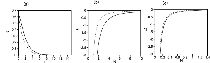
Figure 2: (a) A typical example of the 3D ground state, shown in terms of $\chi(r)\equiv r\left|\psi(r)\right|$, produced by the GPE (22), as per Ref. HS1 , without the external trap ($\Omega=0$), for $U_{0}=0.8$ and $\mu=-0.225$. Panels (b) and (c) display curves $\mu(N)$ for the ground-state families with $U_{0}=0.8$ and $0.1$. These strengths of the attractive potential are, respectively, larger and smaller than the critical value $1/4$ (see Eq. (6)) for the linear Schrödinger equation (15). Here, solid and dashed curves depict, respectively, the numerical results and analytical approximation given by Eqs. (28) and (29) (in panels (b) and (c), the curves follow scaling $\mu\sim N^{-2}$, which is an exact property of Eq. (22)). In particular, the analytical approximation predicts $N(\mu=-0.225)=5.30$ for $U_{0}=0.8$ (the solution shown in (a)), while the numerically found counterpart of this value is $N_{\mathrm{num}}(\mu=-0.225)=6.26$. The convergence of the numerical and analytical curves for $N(\mu)$ at $\mu\rightarrow 0$ corresponds to the fact that Eq. (28) gives exact solution (17) in this limit.

The analytical approximation (28) suggests an estimate for the radial size of the GS created by the repulsive nonlinearity:

$$r_{\mathrm{GS}}^{2}\equiv\frac{4\pi}{N}\int_{0}^{\infty}\left|\psi(r)\right|^{2}r^{4}dr=\frac{N^{2}}{2\pi^{2}U_{0}^{2}}.$$ (31)

It is relevant to rewrite this estimate in terms of physical units, as per Eqs. (10), (11), and (14):

$$\left(r_{\mathrm{GS}}\right)_{\mathrm{ph}}\equiv r_{0}r_{\mathrm{GS}}=\frac{2\sqrt{2}\left(\hbar^{2}a_{s}+md^{2}\right)N_{\mathrm{ph}}}{m\left(U_{0}\right)_{\mathrm{ph}}}.$$ (32)

Note that arbitrary spatial scale $r_{0}$, which was used in rescalings (10) and (11), cancels out in Eq. (11). Thus, GPE (22) uniquely predicts the radius of the restored GS, in terms of physical parameters of the model.

It is natural that $r_{\mathrm{GS}}$, given by Eq. (32), shrinks to zero in the limit of vanishing nonlinearity, which is tantamount to $N_{\mathrm{ph}}\rightarrow 0$, implying the onset of the collapse in the framework of the linear Schrödinger equation. Note also too that, if the contribution from by the dipole-dipole interactions ($\sim d^{2}$) dominates over the contact interactions in Eq. (32) ($md^{2}\gtrsim\hbar^{2}a_{s}$), the latter result strongly simplifies, taking into regard Eq. (7): $\left(r_{\mathrm{GS}}\right)_{\mathrm{ph}}=\left(\sqrt{2}d/|Q|\right)N_{\mathrm{ph}}$. Then, for $Q$ equal to the elementary charge, $d\sim 1$ Debye, and $N_{\mathrm{ph}}\sim 10^{5}$, the latter estimate predicts the GS with radius $\sim 3$ $\mathrm{\mu}$m. This result upholds the self-consistency of the model, as the mean-filed approximation (and the respective GPE) are definitely applicable for scales $\gtrsim 1$ $\mathrm{\mu}$m BEC .

It is worthy to stress that Eq. (8), which does not include the trapping potential, predicts the GS with the finite norm at $U_{0}<1/4$, as the norm of the corresponding stationary solutions to the linear equation (15), see Eqs. (16) and (17), diverges at $\Omega=0$. Lastly, simulations of Eq. (8) with random perturbations added to the stationary solutions demonstrate that the GS is always dynamically stable HS1 . The stability agrees too with the anti-Vakhitov-Kolokolov criterion, $d\mu/dN>0$, which is a necessary stability condition for localized states supported by self-repulsive nonlinearities anti (the original Vakhitov-Kolokolov criterion, $d\mu/dN<0$, is the necessary stability condition in the case of self-attraction VK ; Berge' ) .

II.3 The quantum phase transition induced by the Lee-Huang-Yang (LHY) correction to the mean-field theory

The singularity $\sim r^{-1}$ of the stationary wave function at $r\rightarrow 0$, as seen in Eqs. (24) and (26), suggests that, although the singularity is integrable, as the respective 3D integral for the total norm converges, the LHY correction LHY to the mean-field theory, which is relevant for higher values of the condensate’s density, must be taken into regard. As shown in Ref. Petrov ; AP , the scaled GPE with this correction, represented by coefficient $g_{\mathrm{LHY}}>0$, is

$$i\psi_{t}=-\frac{1}{2}\left(\nabla^{2}+\frac{U_{0}}{r^{2}}\right)\psi+\left|\psi\right|^{2}\psi+g_{\mathrm{LHY}}\left|\psi\right|^{3}\psi.$$ (33)

Then, the asymptotic form of the stationary wave function at $r\rightarrow 0$, which was found above in the form determined by the cubic term in Eq. (22), $\Phi(r)\approx\sqrt{U_{0}/2}r^{-1}$, is replaced by

$$\Phi_{\mathrm{LHY}}(r)\approx\left(U_{0}/2-1/9\right)^{1/3}r^{-2/3},$$ (34)

under the condition of $U_{0}>2/9$, while at $0<U_{0}<2/9$ the asymptotic form is determined by the linearization of Eq. (33), leading to the same result as given by Eqs. (17) and (18) with $\sigma=\sigma_{-}$ (and $U_{l}$ replaced by $U_{0}$):

$$\Phi_{\mathrm{LHY}}(r)\approx\Phi_{0}r^{-\left(1/2-\sqrt{1/4-U_{0}}\right)},$$ (35)

where $\Phi_{0}$ is an arbitrary constant in terms of the expansion at $r\rightarrow 0$. Note that the wave function with asymptotic form $r^{-\sigma_{+}}$, which corresponds to the GS in the linear Schrödinger equation, is incompatible with the presence of the LHY term in Eq. (33), although power $-2/3$ in expression (33) coincides, at the critical point, $U_{0}=2/9$, with $\sigma_{+}$, rather than $\sigma_{-}$.

Thus, the jump from the asymptotic form (35), produced by the linear Schrödinger equation, to one (34) generated by the LHY term at $U_{0}=2/9$ (in particular, the jump between $\sigma_{-}$ and $\sigma_{+}$), takes place at $U_{0}=2/9$, which is a signature of a quantum phase transition. Examples of such phase transitions were studied in many-body settings Grisha and in many other systems other1 -other5 .

Lastly, the LHY term may stabilize the bosonic gas pulled to the center by potential (1) even in the case of the effective attractive interaction, which is possible in a binary condensate, with intrinsic self-repulsion in each components, and dominating attraction between them, as proposed in Refs. Petrov and AP , and realized experimentally in the form of “quantum droplets” (in the binary condensate of ³⁹K) in Refs. droplet1 -droplet3 . For the symmetric mixture, with equal wave functions of the two components, the effective GPE takes the form of Eq. (33) with the opposite sign in front of the cubic term. This model may be a subject for special consideration.

II.4 The two-dimensional ground state created by the quintic self-repulsive nonlinearity

As mentioned above, the GPE in the form of Eq. (8) may be relevant, as a physical model, in 2D too. However, the 2D version of norm (5) of the wave function with asymptotic form $\sim r^{-1}$ at $r\rightarrow 0$, which follows from this equation (see Eq. (28)), logarithmically diverges at small $r$. This means that, the cubic self-repulsion is not strong enough to suppress the collapse in the 2D geometry. On the other hand, the GPE may also include the quintic repulsive term accounting for three-body collisions, provided that the collisions do not give rise to conspicuous losses 3-body1 ; 3-body2 .

The 2D GPE can be derived from the underlying 3D version if tight confinement, with the respective harmonic-oscillator length, $a_{\perp}$, is imposed in direction $z$ by the trapping harmonic-oscillator potential, reducing the effective dimension to that of the plane with remaining coordinates $\left(x,y\right)$ Shlyap -Delgado . In particular, if the dominating quintic terms appears in the 3D GPE with coefficient $g_{5}$, the reduction to the 2D equation replaces it by $\left(\sqrt{3}\pi a_{\perp}^{2}\right)^{-1}g_{5}$.

In the scaled form, the 2D equation it written in the polar coordinates, $\left(r,\theta\right)$, as

$$i\psi_{t}=-\frac{1}{2}\left(\psi_{rr}+\frac{1}{r}\psi_{r}+r+\frac{1}{r^{2}}\psi_{\theta\theta}+\frac{U_{0}}{r^{2}}\right)\psi+\left|\psi\right|^{4}\psi.$$ (36)

Stationary solutions to Eq. (36) (not only the GS, but also for states carrying the angular momentum) are looked for as

$$\psi_{\mathrm{2D}}\left(r,t\right)=e^{-i\mu t+il\theta}r^{-1/2}\chi(r),$$ (37)

where integer $l$ is the azimuthal quantum number, cf. Eq. (24). The substitution of this ansatz in Eq. (36) yields an equation for real $\chi_{\mathrm{2D}}(r)$:

$$\mu\chi=-\frac{1}{2}\left[\chi^{\prime\prime}+\left(U_{l}^{\mathrm{(2D)}}+\frac{1}{4}\right)r^{-2}\chi\right]+r^{-2}\chi^{5},$$ (38)

with $U_{l}^{\mathrm{(2D)}}\equiv U_{0}-l^{2}$, cf. Eq. (19). Note that, unlike the 3D case, in 2D nonlinear model the analysis is possible equally well for $l=0$ (the GS) and $l\geq 1$.

The expansion of the solution to Eq. (38) at $r\rightarrow 0$ yields

$$\chi=\left[\frac{1}{2}\left(U_{l}^{\mathrm{(2D)}}+\frac{1}{4}\right)\right]^{1/4}+\chi_{1}r^{s},$$ (39)

where $s=\left(1/2\right)\left(1+\sqrt{5+16U_{l}^{\mathrm{(2D)}}}\right)$, and $\chi_{1}$ is an arbitrary constant in terms of this expansion, cf. Eq. (26) in the 3D case. The solution with a finite norm exists at $U_{l}^{\mathrm{(2D)}}>-1/4$, representing, at $U_{l}^{\mathrm{(2D)}}>0$, the suppression of the collapse and creation of the GS ($l=0$), or the state with $l\geq 1$, by the quintic self-repulsive term.

Combining the 2D asymptotic form (39), valid at $r\rightarrow 0$, and the obvious approximation valid at $r\rightarrow\infty$, $\chi_{\mathrm{2D}}\approx\chi_{0}\exp\left(-\sqrt{-2\mu}r\right)$, one derives an interpolation formula for the GS, and the dependence $\mu(N)$ following from it, cf. Eqs. (28) and (29) in the 3D case:

$$\psi_{\mathrm{2D}}\left(r,t\right) = \left[\frac{1}{2}\left(U_{l}^{\mathrm{(2D)}}+\frac{1}{4}\right)\right]^{1/4}e^{-i\mu t+il\theta}r^{-1/2}e^{-\sqrt{-2\mu}r},$$

$$\mu = -\left(U_{l}^{\mathrm{(2D)}}+\frac{1}{4}\right)\left(\frac{\pi}{2N}\right)^{2},$$ (40)

Similar to the situation in the 3D case, Eq. (40) gives an exact wave function with a divergent norm in the limit of $\mu\rightarrow-0$,

$$\psi_{\mathrm{2D}}^{(\mu=0)}(r)=\left[\frac{1}{2}\left(U_{l}^{\mathrm{(2D)}}+\frac{1}{4}\right)\right]^{1/4}e^{il\theta}r^{-1/2},$$ (41)

cf. Eq. (30).

The approximation (40) makes it possible to define the rms radial size of the two-dimensional GS, cf. Eq. (31) in the 3D case:

$$r_{\mathrm{GS}}^{\mathrm{(2D)}}\equiv\sqrt{\frac{2\pi}{N}\int_{0}^{\infty}\left|\psi_{\mathrm{2D}}(r)\right|^{2}r^{3}dr}=\frac{N}{\pi\sqrt{\left(U_{l}^{\mathrm{(2D)}}+1/4\right)}}.$$ (42)

Note that the quintic term supports the GS in 2D even at $0<-U_{l}^{\mathrm{(2D)}}<1/4$, when the central potential is repulsive. The correctness of this counter-intuitive conclusion is corroborated by the above-mentioned fact that the analytical approximation (40) gives exact solution (41) for $\mu\rightarrow 0$, including the case of $0<-U_{l}^{\mathrm{(2D)}}<1/4$.

An example of the stable GS, and curves $\mu(N)$ for the GS in 2D are displayed, along with the analytical approximation (40), in Fig. 3 (referring to $l=0$, although it actually makes no difference in the plots). The $\mu(N)$ curves are shown for both signs of the central potential, $U_{0}=-0.18$ and $U_{0}=0.05$. Simulations of the perturbed evolution in the framework of Eq. (36) confirm stability of the GS families.

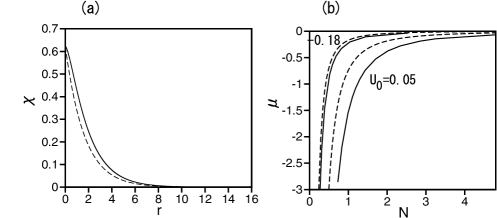
Figure 3: (a) The radial profile of the ground state in the 2D model with the quintic nonlinearity, for $U_{0}=0.05$ and $\mu=-0.1867$. (b) Curves $\mu(N)$ for the ground states with $U_{0}=-0.18$ and $U_{0}=0.05$. In both panels (shown as per Ref. HS1 ), the numerical results and the respective analytical approximation (40) are depicted by the continuous and dashed curves, respectively. The convergence of the numerical and analytical curves for $N(\mu)$ at $\mu\rightarrow-0$ corresponds to the fact that Eq. (40) gives the exact solution (41) in this limit.

Generally, the results for the 2D model are more formal than those summarized above for 3D, as the realization of the dominant quintic nonlinearity in BEC is problematic, in experimentally relevant settings. On the other hand, the LHY correction to the GPE is also sufficient to provide the suppression of the quantum collapse and restoration of the GS in the 2D setting. The same dimension-reduction procedure as outlined above, will replace the original LHY coefficient in 3D equation (33) by $\sqrt{2/5}\pi^{-3/4}a_{\perp}^{-3/2}g_{\mathrm{LHY}}$. Finally, the quartic LHY term determines the asymptotic form of the wave functions at $r\rightarrow 0$ as $\sim r^{-2/3}$, which provides for the convergence of the 2D norm, i.e., it secures the existence of the GS in the 2D model including the LHY term.

II.5 A challenging issue: the Fermi gas pulled to the center

An interesting possibility is to elaborate the 3D model for the gas of fermions pulled to the center by potential (1). In a rigorous form, this is a challenging problem, as the dynamical theory for Fermi gases cannot be reduced to a simple mean-field equation Fermi . Nevertheless, there is a relatively simple approach to the description of stationary states in a sufficiently dense gas, which is based on a time-independent equation for the real fermionic wave function, $\Phi\left(\mathbf{r}\right)$ Minguzzi ; SKA ; Luca , with a nonlinear term of power $7/3$ generated by the density-functional approximation, even in the absence of direct interaction between the fermions, which is forbidden by the Pauli principle. In the scaled form, this equation, including potential (1) and chemical potential $\mu$, is

$$\mu\Phi=-\frac{1}{3}\nabla^{2}\Phi+\Phi^{7/3}-\frac{U_{0}}{2r^{2}}\Phi.$$ (43)

The asymptotic form of the solution to Eq. (43) at $r\rightarrow 0$ is

$$\Phi(r)=\sqrt{\left(3+4U_{0}\right)/8}r^{-3/2}+O\left(r^{1/2}\right).$$ (44)

This result demonstrates a problem similar to the one stressed above in the case of the 2D model with the cubic nonlinearity: the substitution of expression (44) in the 3D integral (5) for the norm of the wave function leads to the logarithmic divergence at $r\rightarrow 0$, hence the relatively weak nonlinearity in Eq. (43) is insufficient for the suppression of the 3D quantum collapse of the Fermi gas pulled to the center by potential (1), and a more sophisticated analysis is necessary in this case.

III The three-dimensional model with cylindrical symmetry

The presentation in this section follows the original analysis reported in Ref. HS2 .

III.1 Formulation of the model

The previous section addressed the most fundamental spherically symmetric configuration in the 3D space. Because the geometry plays a crucially important role in determining properties of the bound states produced by the model, it is interesting to consider physically relevant settings in 3D with the spatial symmetry reduced from spherical to a lower one. In particular, it is possible to consider the model in which a strong uniform external field is applied to the quantum gas, so that all the dipole moments, carried by the particles, are polarized not towards the center, but in a fixed direction ($z$), so that $\mathbf{d}=d\mathbf{e}_{z}$. This configuration gives rise the cylindrically symmetric potential of the interaction of the dipolar particle with the fixed attractive center:

$$U(\mathbf{r})=-\mathbf{d}\cdot\mathbf{E}_{Q}=-\frac{1}{2}U_{0}r^{-2}\cos\theta,$$ (45)

where $\cos\theta\equiv z/r$.

If the polarizing external field is electric, it acts on the central charge too. For this reason, a more relevant situation corresponds to the case when the ultracold gas is composed of Hund A type of molecules, with mutually locked electric and magnetic dipoles. Then, external uniform magnetic field may be employed to align the dipoles in the fixed direction Santos .

The 3D GPE with potential (45) is

$$i\frac{\partial\psi}{\partial t}=-\frac{1}{2}\left(\nabla^{2}\psi+\frac{U_{0}}{r^{2}}\cos\theta\right)\psi+|\psi|^{2}\psi.$$ (46)

Along with the consideration of the GS, it is also relevant to construct eigenmodes carrying the orbital angular momentum, which corresponds to the azimuthal quantum number, $m$:

$$\psi=e^{-i\mu t}e^{im\varphi}\Phi(r,\theta),$$ (47)

where the spherical coordinates are used again, cf. Eq. (16), and real eigenmode $\phi$ should be found as a solution of the equation following from the substitution of ansatz (47) in Eq. (46):

$$\mu\Phi=-\frac{1}{2}\left[\frac{\partial^{2}}{\partial r^{2}}+\frac{2}{r}\frac{\partial}{\partial r}-\frac{m^{2}}{r^{2}\sin^{2}\theta}+\frac{1}{r^{2}\sin\theta}\frac{\partial}{\partial\theta}\left(\sin\theta\frac{\partial}{\partial\theta}\right)+\frac{U_{0}}{r^{2}}\cos\theta\right]\Phi+\Phi^{3}.$$ (48)

III.2 The linear Schrödinger equation with the cylindrical symmetry

The analysis of the present model should start with identifying conditions for the existence of the GS in the respective linear Schrödinger equation, obtained by dropping the cubic term in Eq. (48). At $r\rightarrow 0$, an asymptotic solution to the linear equation is looked for as

$$\Phi\left(r,\theta\right)=r^{-\sigma}\chi_{\mathrm{lin}}(\theta).$$ (49)

The substitution of ansatz (49) in the linearized version of Eq. (48) and dropping term $\mu\Phi$, which is negligible for the asymptotic analysis at $r\rightarrow 0$, leads to an equation that can be written in terms of $\xi\equiv\cos\theta$:

$$\frac{d}{d\xi}\left(\left(1-\xi^{2}\right)\frac{d\chi_{\mathrm{lin}}}{d\xi}\right)+\left(\sigma^{2}-\sigma-\frac{m^{2}}{1-\xi^{2}}+U_{0}\xi\right)\chi_{\mathrm{lin}}(\xi)=0.$$ (50)

For $U_{0}=0$, equation (50) with integer values

$$\sigma=l+1$$ (51)

may be solved in terms of the associated Legendre functions, $l\geq m$ being the orbital quantum number. Note that the singular wave function (49) is 3D-normalizable, at $r\rightarrow 0$, for $\sigma<3/2$, i.e., as it follows from Eq. (51), solely for the GS, with $m=l=0$ and $\sigma=1$.

The onset of the quantum collapse is signalled by a transition in Eq. (50) from real eigenvalues $\sigma$ to complex ones. Because the effective eigenvalue in the equation is $\epsilon\equiv\sigma^{2}-\sigma$, i.e., $\sigma=(1+\sqrt{1+4\epsilon})/2$, the transition to complex $\sigma$ happens at point $\epsilon=-1/4$ (i.e., $\sigma=1/2$). At $U_{0}\neq 0$, Eq. (50) cannot be solved in terms of standard special functions. A result of a numerical solution is displayed in Fig. 4. It demonstrates that, for given azimuthal quantum number $m$, eigenvalue $\sigma$ decreases, with the increase of $U_{0}$ from zero to some critical value $\left(U_{0}\right)_{\mathrm{cr}}$, from $\sigma\left(U_{0}=0\right)=m+1$ to $\sigma\left(U_{0}=\left(U_{0}\right)_{\mathrm{cr}}\right)=1/2$. For lowest values of $m$, the numerically found critical values of the potential strength, at which $\sigma=1/2$ is attained are

$$\left(U_{0}\right)_{\mathrm{cr}}(m=0,1,2)=1.28,7.58,19.06.$$ (52)

In the framework of the linear Schrödinger equation, the quantum collapse takes place at $U_{0}>\left(U_{0}\right)_{\mathrm{cr}}(m)$.

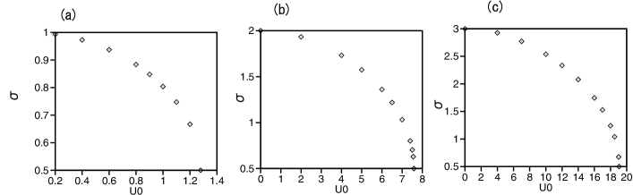
Figure 4: Eigenvalue $\sigma$ of the singular eigenmode (49), generated, as per Ref. HS2 , by the numerical solution of linear equation (50), vs. strength $U_{0}$ of the attractive potential, for three values of the azimuthal quantum number: (a) $m=0$, (b) $m=1$, (c) $m=2$. The eigenmode disappears, signaling the onset of the quantum collapse, at $U_{0}>\left(U_{0}\right)_{\mathrm{cr}}(m)$, see Eq. (52), where $U_{0}=\left(U_{0}\right)_{\mathrm{cr}}(m)$ corresponds to $\sigma=1/2$.

It is relevant to compare critical values (52) of the strength of the axisymmetric potential with those given by Eq. (19) for the spherically isotropic one:

$$\left(U_{0}\right)_{\mathrm{cr}}^{\mathrm{(iso)}}(m=0,1,2)=\frac{1}{4}+m(m+1)\equiv 0.25,2.25,6.25.$$ (53)

The comparison naturally shows that the critical strengths are much lower for the spherical potential, which provides stronger pull to the center.

III.3 Suppression of the quantum collapse by the repulsive nonlinearity under the cylindrical symmetry

As well as in the isotropic setting, cf. Eq. (24), the repulsive cubic term in Eq. (48) may balance the attractive potential $\sim-r^{-2}$ if, at $r\rightarrow 0$, the wave function contains the singular factor $r^{-1}$ (rather than generic $r^{-\sigma}$ in Eq. (49)). Then, the substitution of

$$\Phi(r,\theta)=r^{-1}\chi(r,\theta),$$ (54)

transforms Eq. (48) into the following equation:

$$\mu\chi=-\frac{1}{2}\left[\frac{\partial^{2}\chi}{\partial r^{2}}+\frac{1-\xi^{2}}{r^{2}}\frac{\partial^{2}\chi}{\partial\xi^{2}}-\frac{2\xi}{r^{2}}\frac{\partial\chi}{\partial\xi}+\left(U_{0}\xi-\frac{m^{2}}{1-\xi^{2}}\right)\frac{\chi}{r^{2}}\right]+\frac{\chi^{3}}{r^{2}}$$ (55)

(recall $\xi\equiv\cos\theta$). Note that Eq. (54) makes it possible to write the norm of the 3D wave function as

$$\frac{N}{2\pi}=\int_{0}^{\infty}r^{2}dr\int_{0}^{\pi}\sin\theta d\theta\left|\psi\left(r,\theta\right)\right|^{2}=\int_{0}^{\infty}dr\int_{-1}^{+1}d\xi\chi^{2}\left(r,\xi\right).$$ (56)

To analyze solutions to Eq. (55) at $r\rightarrow 0$, one may expand them as

$$\chi(r,\xi)=\chi_{0}(\xi)+\chi_{1}(\xi)r^{s/2},$$ (57)

assuming $s>0$, which leads to the following equation for $\chi_{0}(\xi)$, that does not admit an exact solution:

$$\left(1-\xi^{2}\right)\frac{d^{2}\chi_{0}}{d\xi^{2}}-2\xi\frac{d\chi_{0}}{d\xi}+\left(U_{0}\xi-\frac{m^{2}}{1-\xi^{2}}\right)\chi_{0}-\chi_{0}^{3}=0,$$ (58)

cf. Eq. (50).

Bound states produced by Eq. (55) were found by means of numerical methods in Ref. HS2 . Typical profiles of solutions for function $\chi\left(r,\xi\right)$, generated  by Eq. (55), are displayed in Fig. 5, for $m=0,1,2$ and fixed norm, $N=2\pi$.

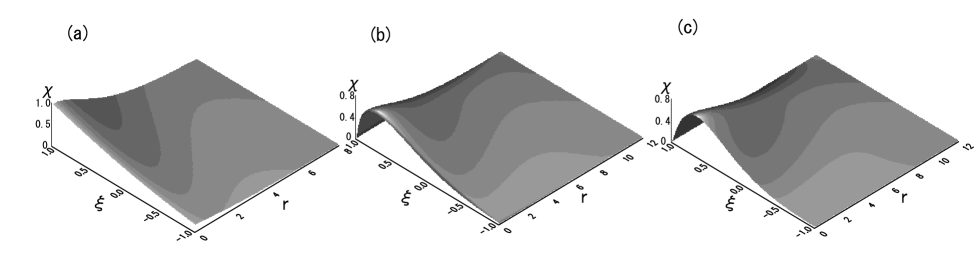
Figure 5: Typical profiles of real function $\chi(r,\xi)$, produced, in Ref. HS2 , by the numerical solution of Eq. (55), which determines the shape of the bound state with the reduced (cylindrical) symmetry, as per Eq. (54): (a) $m=0,U_{0}=3$; (b) $m=1,U_{0}=8.5$; (c) $m=2,U_{0}=20$. The solutions are subject to normalization $N=2\pi$, see Eq. (56).

A crude analytical form of the solutions is provided by the Thomas-Fermi approximation (TFA), which neglects all derivatives in Eq. (55) BEC :

$$\chi_{\mathrm{TFA}}^{2}\left(r,\xi\right)=\left\{\begin{array}[]{c}\frac{1}{2}U_{0}\xi-\frac{m^{2}}{2\left(1-\xi^{2}\right)}-|\mu|r^{2},~{}~{}\mathrm{at}~{}~{}r^{2}<\frac{1}{2|\mu|}\left(U_{0}\xi-\frac{m^{2}}{1-\xi^{2}}\right),\\ 0,~{}~{}\mathrm{at}~{}~{}r^{2}\geq\frac{1}{2|\mu|}\left(U_{0}\xi-\frac{m^{2}}{1-\xi^{2}}\right).\end{array}\right.$$ (59)

Actually, this approximation for $m\geq 1$ exists only for $U_{0}>\left(3\sqrt{3}/2\right)m^{2}$ (otherwise, Eq. (59) yields $\chi_{\mathrm{TF}}^{2}\equiv 0$).

Families of the bound states with different quantum numbers $m$ are presented in Fig. 6 by a set of curves showing the chemical potential, $\mu$, versus nonlinearity strength, $U_{0}$, for a fixed norm ($N=N_{0}\equiv 2\pi$; producing the results for a fixed norm is sufficient, as the scaling invariance of Eq. (55) implies an exact property, $\mu\left(U_{0},N\right)=\left(N/N_{0}\right)^{-2}\mu\left(U_{0},N_{0}\right)$, the same as mentioned above for the isotropic configuration). Figures 6(b) and (c) display the $\mu(U_{0}$) dependences in relatively narrow intervals of values of $U_{0}$, to stress that the dependences are obtained above the critical values for the linear Schrödinger equation given by Eq. (52), where the linear equation fails to produce any bound state.

TFA based on Eq. (59) makes it possible to predict the $\mu\left(U_{0}\right)$ dependence for the GS ($m=0$) in an analytical form:

$$\mu_{\mathrm{TFA}}^{\mathrm{(GS)}}=-\left(2/225\right)U_{0}^{3}.$$ (60)

As seen in Fig. 6(a), this simple approximation is reasonably close to its numerically found counterpart.

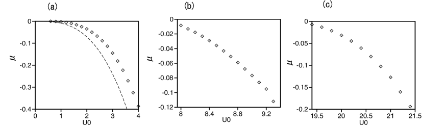
Figure 6: Panels (a), (b), (c) display, respectively, the chemical potential of the bound states with azimuthal quantum numbers $m=0,1,2$, vs. the strength of the attractive potential, $U_{0}$, of the potential (45), with the the reduced (cylindrical) symmetry, and for the fixed norm, $N=2\pi$, as obtained in Ref. HS2 . The dashed curve in (a) additionally shows dependence (60) predicted by the TF approximation.

Lastly, the stability of the bound states against perturbations was verified in Ref. HS2 by direct simulations of the underlying GPE (46), demonstrating complete stability that the families of the states for $m=0,1,$ and $2$.

IV The two-component system in three dimensions: the suppression of the quantum collapse in miscible and immiscible settings

This section summarizes results of the analysis reported in Ref. HS3 .

IV.1 The formulation of the model and analytical considerations

The generalization of basic model (22) for a binary bosonic gas, with component wave functions $\psi_{1}$ and $\psi_{2}$, is provided by the system of nonlinearily coupled GPEs:

$$i\frac{\partial\psi_{1}}{\partial t} = -\frac{1}{2}\nabla^{2}\psi_{1}+(|\psi_{1}|^{2}+\gamma|\psi_{2}|^{2})\psi_{1}-\frac{V_{0}}{r^{2}}\psi_{1}~{},$$

$$i\frac{\partial\psi_{2}}{\partial t} = -\frac{1}{2}\nabla^{2}\psi_{2}+(\gamma|\psi_{1}|^{2}+|\psi_{2}|^{2})\psi_{2}-\frac{V_{0}}{r^{2}}\phi_{2}~{}$$

(for the consistency with Ref. (HS2 ), parameter $V_{0}\equiv U_{0}/2$ is now used as the strength of the potential pulling particles to the center), where $\gamma$ is the relative strength of the inter-component repulsion, and coefficients of the self-repulsion are scaled to be $1$.

Spherically symmetric bound states with chemical potentials $\mu_{n}<0$, $n=1,2$, of the two components are looked for as

$$\psi_{n}\left(r,t\right)=\frac{\chi_{n}(r)}{r}\exp\left(-i\mu_{n}t\right),$$ (62)

with real radial functions $\chi_{n}(r)$ obeying the coupled equations,

$$\mu_{1}\chi_{1} = -\frac{1}{2}\chi_{1}^{\prime\prime}-\frac{V_{0}}{r^{2}}\chi_{1}+\left(\chi_{1}^{2}+\gamma\chi_{2}^{2}\right)\frac{\chi_{1}}{r^{2}},$$

$$\mu_{2}\chi_{2} = -\frac{1}{2}\chi_{2}^{\prime\prime}-\frac{V_{0}}{r^{2}}\chi_{2}+\left(\chi_{2}^{2}+\gamma\chi_{1}^{2}\right)\frac{\chi_{2}}{r^{2}},$$

cf. Eqs. (24) and (25). In terms of these functions, the norms of the components are

$$N_{n}\equiv\int\left|\phi_{n}(\mathbf{r})\right|d\mathbf{r}=4\pi\int_{0}^{\infty}\left[\chi_{n}(r)\right]^{2}dr,$$ (64)

and the rms radial size of the trapped mode in each component is defined as

$$\left\langle r_{n}^{2}\right\rangle=\frac{\int_{0}^{\infty}\left[\chi_{n}(r)\right]^{2}r^{2}dr}{\int_{0}^{\infty}\left[\chi_{n}(r)\right]^{2}dr},$$ (65)

cf. Eq. (31).

An expansion of solutions to Eqs. (LABEL:stat) at $r\rightarrow 0$ is looked for as

$$\chi_{n}(r)=\chi_{n}^{(0)}\left[1-c_{n}^{(1)}r^{s/2}-c_{n}^{(2)}r^{s/2+2}+\cdots-d_{n}^{(1)}r^{2}-d_{n}^{(2)}r^{4}+\cdots\right],$$ (66)

with $s>0$, cf. Eq. (26) (here, $c_{1}\neq c_{2}$ is possible, but power $s$ must be the same for $\chi_{1}$ and $\chi_{2}$), which leads to a system of algebraic equations for leading-order coefficients $\chi_{n}^{(0)}$:

$$\chi_{1}^{(0)}\left[\left(\chi_{1}^{(0)}\right)^{2}+\gamma\left(\chi_{2}^{(0)}\right)^{2}\right] = V_{0}\chi_{1}^{(0)},$$

$$\chi_{2}^{(0)}\left[\left(\chi_{2}^{(0)}\right)^{2}+\gamma\left(\chi_{1}^{(0)}\right)^{2}\right] = V_{0}\chi_{2}^{(0)}.$$

Equations (LABEL:chichi) give rise to solutions of two types, corresponding to mixed and demixed states in the binary gas:

$$\chi_{1}^{(0)} = \chi_{2}^{(0)}\equiv\chi_{\mathrm{mix}}^{(0)}=\sqrt{V_{0}/\left(1+\gamma\right)};$$ (68)

$$\chi_{1}^{(0)} \equiv \chi_{\mathrm{demix}}^{(0)}=\sqrt{V_{0}},~{}\chi_{2}^{(0)}=0.$$ (69)

The numerical analysis performed in Ref. HS2 has demonstrates that demixed modes do not exist at $\gamma<1$, when the mutual repulsion is weaker than the self-repulsive nonlinearity, while mixed ones are completely unstable in the opposite case, $\gamma>1$. Thus, unlike other systems featuring the miscibility-immiscibility transitions misc0 -misc1 , in the present situation the transition point is not shifted, under the action of the confining potential, from the commonly known free-space point, $\gamma=1$ Mineev .

Further analysis demonstrates a change in the structure of the $r$-dependent corrections in Eq. (66) for the miscible system, with $\gamma<1$: at $V_{0}<1/2$, the dominant terms are $\sim r^{\left(1+\sqrt{1+16V_{0}}\right)/2}$, while at $V_{0}>1/2$ these are terms $\sim r^{2}$. This break of analyticity, which happens, with the increase of $V_{0}$, at $V_{0}=1/2$, implies that a weak quantum phase transition happens at this value of $V_{0}$, although the well-defined GS exists equally well at $V_{0}<1/2$ and $V_{0}>1/2$. Precisely at $V_{0}=1/2\equiv\left(V_{0}\right)_{\mathrm{phase-trans}}$, expansion (66) is replaced by

$$\chi_{n}(r)=\frac{1}{\sqrt{2\left(1+\gamma\right)}}\left[1+\frac{\mu_{1}+\mu_{2}}{4}r^{2}\ln\left(\frac{r_{0}}{r}\right)+(-1)^{n}\frac{1+\gamma}{4\gamma}\left(\mu_{1}-\mu_{2}\right)r^{2}\right].$$ (70)

Note that the present phase transition is weak in comparison with the above-mentioned one, driven by the LHY correction to the mean-field theory, which gives rise to the jump between the different asymptotic forms of the wave function, given by Eqs. (34) and (35). For the comparison with the present setting, based on the binary BEC, especially relevant are previously investigated phase transitions in binary fluids fluids . Recall that the onset of the quantum collapse in the linear version of the model occurs at the critical value$\left(V_{0}^{(\mathrm{cr})}\right)_{1}\equiv(1/2)\left(U_{0}\right)_{\mathrm{cr}}^{(\mathrm{3D})}=1/8$ LL , which is a quarter of the value of the potential’s strength at the phase-transition point, $\left(V_{0}\right)_{\mathrm{phase-trans}}=1/2$.

Lastly, at $r\rightarrow\infty$ Eqs. (LABEL:stat) yield an exponential asymptotic form of the solution,

$$\chi_{n}(r)\approx\chi_{n}^{(\infty)}\left(1-\frac{V_{0}}{\sqrt{-2\mu_{n}}r}\right)\exp\left(-\sqrt{-2\mu_{n}}r\right),$$ (71)

where constants $\chi_{n}^{(\infty)}$ are indefinite in terms of the asymptotic expansion at $r\rightarrow\infty$.

IV.2 Numerical and additional analytical results for trapped binary modes

IV.2.1 Mixed ground states

Figure 7(a) shows a typical profile for the mixed GS produced by a numerical solution of Eq. (LABEL:stat) at $V_{0}=1$ for $\gamma=0.9$ and equal norms of the two components, $N_{1}=N_{2}=4\pi$.

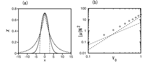
Figure 7: (a) The numerically found profile of wave functions $\chi_{1}(r)=\chi_{2}(r)$, at $V_{0}=1$, $\gamma=0.9$, and $N_{1}=N_{2}=4\pi$, of the GS in the miscible binary system, as found in Ref. HS3 , and its comparison with the analytical approximation given by Eq. (72), and TFA based on Eq. (75) (the short- and long-dashed lines, respectively). (b) The chain of rhombuses depicts the numerically found relation between $|\mu|N^{2}$ and $V_{0}$ at $\gamma=0.9$. The short- and long-dashed lines represent the approximations provided by Eqs. (73) and (76), respectively.

The simplest global analytical approximation for the GS wave function is provided by the interpolation, similar to that introduced in the single-component setting, cf. Eq. (28):

$$\chi_{n}(r)\approx\chi_{\mathrm{mix}}^{(0)}e^{-\sqrt{-2\mu_{n}}r}.$$ (72)

The substitution of this interpolation in Eqs. (64) and (65), along with expression (68), leads to predictions for the chemical potentials and squared average radius of the two components as functions of their norms (which are valid too in the case of $N_{1}\neq N_{2}$):

$$\mu_{n} = -2\left[\frac{\pi V_{0}}{(1+\gamma)N_{n}}\right]^{2},$$ (73)

$$\left\langle r_{n}^{2}\right\rangle = \left[\frac{(1+\gamma)N_{n}}{2\pi V_{0}}\right]^{2}.$$ (74)

Comparison of expression (73) with numerical results is shown in Fig. 7(b) by the dashed line. This approximation is accurate for sufficiently small $V_{0}$, but becomes inaccurate for large $V_{0}$.

For larger $V_{0}$, TFA can be applied to the mixed balanced mixture, with $N_{1}=N_{2}\equiv N$, which yields (for $\chi_{1}=\chi_{2}\equiv\chi$)

$$\chi_{\mathrm{TFA}}(r)=\left\{\begin{array}[]{c}\sqrt{\left(V_{0}+\mu r^{2}\right)/\left(1+\gamma\right)}\,,~{}~{}\mathrm{at}~{}~{}r<R_{0}\equiv\sqrt{V_{0}/(-\mu)},\\ 0,~{}~{}\mathrm{at}~{}~{}r>R_{0}~{},\end{array}\right.$$ (75)

cf. TFA for the potential with the cylindrical symmetry, given by Eq. (59). The substitution of approximation (75) in Eqs. (5) and (65) yields the predictions for the chemical potential and effective size of the GS:

$$\mu_{\mathrm{TFA}} = -\frac{64\pi^{2}V_{0}^{3}}{9(1+\gamma)^{2}N^{2}},$$ (76)

$$\left\langle r_{\mathrm{TFA}}^{2}\right\rangle = \frac{5}{\pi^{3}}\left[\frac{3\left(1+\gamma\right)N}{16V_{0}}\right]^{2}\equiv\frac{5}{4\pi}R_{0}^{2}$$ (77)

(recall $R_{0}$ is the TFA cutoff radius defined in Eq. (75)). Analytical approximations (72) and (75) (shown by the short- and long-dashed lines, respectively) are compared to the numerically found profile of the GS in Fig. 7(b). A general conclusion (see details in Ref. HS3 ) is that, quite naturally, TFA works better for larger $V_{0}$, while interpolation (72) is more accurate for smaller $V_{0}$.

Numerically generated profiles of imbalanced mixed GSs are displayed in Fig. 3(a) at $V_{0}=2$ and $\gamma=0.9$ for $N_{1}=4\pi$ and $N_{2}=2\pi$. The imbalanced mixed states with $\mu_{1}\neq\mu_{2}$ and $N_{1}\neq N_{2}$ feature equal values of $\chi_{1,2}(r=0)$, in agreement with Eq. (68).

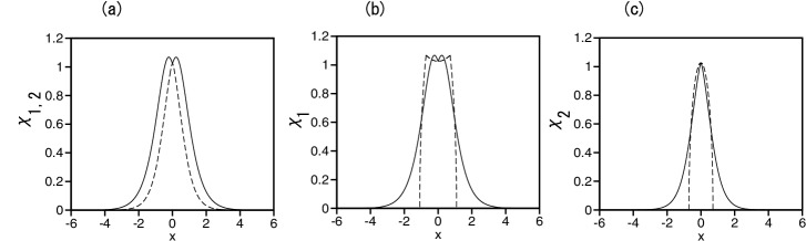
Figure 8: (a) $\chi_{1}$ (continuous) and $\chi_{2}$ (dashed) components of the imbalanced mixed GS of the binary system, at $V_{0}=2$ and $\gamma=0.9$, with $N_{1}=4\pi$ and $N_{2}=2\pi$, as found in Ref. HS3 . (b) and (c): Comparison of the numerical result (continuous lines) with the two-layer TFA (dashed lines, see Eqs. (79) and (80)) for $\chi_{1}(r)$ and $\chi_{2}(r)$.

In the case of the strong pull to the center, $V_{0}\gg 1$, TFA can be generalized for imbalanced states, fixing $\left|\mu_{1}\right|\leq\left|\mu_{2}\right|$ for the definiteness’ sake. Then, TFA is constructed in a two-layer form, technically similar to that applied to the so-called symbiotic gap solitons in Ref. Thawatchai . In the inner layer,

$$r^{2}<r_{0}^{2}\equiv\frac{1-\gamma}{\gamma\mu_{1}-\mu_{2}}V_{0},$$ (78)

both wave functions are different from zero:

$$\chi_{n}^{\mathrm{(inner)}}(r)=\sqrt{\frac{V_{0}}{1+\gamma}-\frac{\gamma\mu_{3-n}-\mu_{n}}{1-\gamma^{2}}r^{2}}.$$ (79)

In the outer layer, only one component is present, in the framework of TFA: $\chi_{2}\equiv 0$,

$$\chi_{1}^{\mathrm{(outer)}}(r)=\left\{\begin{array}[]{c}\sqrt{V_{0}+\mu_{1}r^{2}},~{}\mathrm{at}~{}~{}r_{0}^{2}\leq r^{2}\leq R_{0}^{2}\equiv-V_{0}/\mu_{1},\\ 0,~{}\mathrm{at}~{}~{}r^{2}\geq R_{0}^{2}~{}.\end{array}\right.$$ (80)

Both components of the TFA solution, given by Eqs. (78)-(80), are continuous at $r=r_{0}$ and $r=R_{0}$. The two-layer TFA for a typical imbalanced GS is compared to its numerical counterpart in Figs. 8(b,c).

The analysis reported in Ref. HS3 also includes the consideration of a two-component system with attraction between the components, in the case when only one component is subject to the action of the pull-to-the-center potential, while the other one plays the role of a buffer. In particular, the interpolation, similar to that based on Eq. (72), produces a sufficiently accurate prediction in that case.

IV.2.2 Immiscible ground states

As said above, in the case of $\gamma>1$ relevant states are immiscible ones. The two-layer TFA may be applied to produce an immiscible GS. In the inner layer,

$$r^{2}<r_{0}^{2}=\frac{(\gamma-1)V_{0}}{\gamma\mu_{1}-\mu_{2}},$$

the approximation yields

$$\chi_{1}(r)=\sqrt{V_{0}+\mu_{1}r^{2}},\;\chi_{2}(r)=0.$$ (81)

In the outer layer, which is $r_{0}^{2}<r^{2}<R_{0}^{2}=V_{0}/(-\mu_{2})$, the result is

$$\chi_{1}(r)=0,\;\chi_{2}(r)=\sqrt{V_{0}+\mu_{2}r^{2}},$$ (82)

i.e., TFA predicts complete separation between the components in the immiscible state. Figure 9 compares the approximation to numerical results. Of course, the immiscible components are not completely separated in the numerical solution.

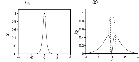
Figure 9: (a) and (b): Comparison of the numerically found profiles for components $\chi_{1}(r)$ and $\chi_{2}(r)$ of the immiscible GS (solid lines) in the binary condensate ($V_{0}=1$, $\gamma=1.2$) with equal norms of both components ($N_{1}=N_{2}=0.8\pi$), and the respective TFA, given by Eqs. (81) and (82), respectively (continuous lines), as per Ref. HS3 . The numerical solution gives widely different values of chemical potentials of the two components in this case: $\mu_{1}=-14.2$, $\mu_{2}=-0.84$.

V The mean-field predictions versus the many-body quantum theory

V.1 Introduction to the section

The analysis presented above was performed in Refs. HS1 -HS3 in the framework of the mean-field theory, i.e., the respective GPEs (possibly including the beyond-mean-field LHY corrections, see Eq. (33)). A relevant issue is comparison of the basic mean-field predictions, such as the suppression of the quantum collapse and creation of the originally missing GS, with the consideration of the many-body system of repulsively interacting quantum bosons, pulled to the center by potential (1), which is taken here as $U(r)=-U_{0}/r^{2}$, i.e., $U_{0}$ in Eq. (1) is replaced by $2U_{0}$, to make the notation consistent with that in Ref. GEA . This problem was addressed in Ref. GEA . Results produced in that work are recapitulated in the present section.

The many-body Hamiltonian representing the setting under the consideration is

$$\hat{H}=-\sum\limits_{j=1}^{N}\left(\frac{\hbar^{2}\nabla_{j}^{2}}{2m}+\frac{U_{0}}{r_{j}^{2}}\right)+\sum\limits_{j<k}^{N}V_{\mathrm{int}}(|\mathbf{r}_{j}-\mathbf{r}_{k}|),$$ (83)

where $\mathbf{r}_{j}$ are coordinates of the $j$-th particle in the 3D space, $m$ is the particle’s mass, and $V_{\mathrm{int}}(r)$ is the potential of the repulsive interaction between the particles. In the framework of the mean-field theory, $V_{\mathrm{int}}(r)$ is characterized solely by the $s$-wave scattering length BEC , while the many-body system should be introduced with a particular form of the interaction potential. Two basic forms of the interaction potential chosen for the analysis are specified below, see Eqs. (88) and (89).

Before introducing the many-body wave function, the single-particle one is adopted as per the following ansatz:

$$f_{1}(r)=r^{\beta}\exp(-\alpha r^{2}),$$ (84)

where $\alpha\geq 0$ determines the inverse localization length, which affects the system’s size and, consequently, the density. Alternatively, $\alpha$ can be interpreted in terms of an effective external harmonic confinement with frequency $\Omega=2\alpha\hbar/m$, cf. Eq. (4). At $r_{j}\rightarrow 0$, the shape of the wave function is controlled by parameter $\beta$ in ansatz (84).

V.2 The single-particle solution

The single-particle problem, defined by Hamiltonian (83) with $N=1$, can be studied by means of the variational method, treating $\alpha$ and $\beta$ in ansatz (84) as variational parameters. In the single-particle sector, the system is steered by the competition of the external potential and kinetic energy, while the interparticle potential, $V_{\mathrm{int}}(|\mathbf{r}_{i}-\mathbf{r}_{j}|)$, does not appear. The variational energy, $E_{\mathrm{var}}^{(1)}=\left[\int f_{1}^{2}(\mathbf{r})\;d\mathbf{r}\right]^{-1}\int f_{1}(\mathbf{r})Hf_{1}(\mathbf{r})d\mathbf{r}$, with $f_{1}$ taken as per Eq. (84), is

$$E^{(1)}=\alpha\left[1-\frac{8U_{0}-1}{2(1+2\beta)}\right].$$ (85)

For a fixed localization size, $\alpha=\mathrm{const}$, this energy is a decreasing function of $\beta$ if $U_{0}$ is smaller than the critical value for the onset of the collapse, $U_{0}=1/8$ – the same which appears in Eq. (6). On the other hand, a metastable state may appear in the many-body system with repulsive interparticle interactions. Actually, it corresponds to the mean-field GS predicted by the solution of the GPE in Ref. HS1 , see further details below

In the framework of the local-density approximation, the chemical potential of the state with uniform density $n$ is take as $\mu_{\mathrm{\hom}}=gn$ , where $g=4\pi\hbar^{2}a_{s}/m$ is the coupling constant. This choice corresponds to the short-range interaction potential determined by the $s$-wave scattering length as per the Born approximation. Further, the chemical potential in the presence of the external field is approximated by the sum of the local chemical potential $\mu_{\mathrm{loc}}=gn$, where, this time, $n$ is a function of the coordinates, rather than a constant, and the external potential,

$$\mu=\mu_{\mathrm{loc}}-\frac{U_{0}}{r^{2}}+\frac{1}{2}m\Omega^{2}r^{2},$$ (86)

where the harmonic-oscillator confinement, with the respective length scale, $a_{\mathrm{ho}}=\sqrt{\hbar/(m\Omega)}$, is added to make the size of the system finite, cf. potential (4) used above. Solving Eq. (86) for the density, one obtains the following density profile:

$$n(r)=\frac{1}{g}\begin{cases}\mu-\frac{1}{2}m\Omega^{2}r^{2}+U_{0}r^{-2},&\mathrm{at\ }r<R_{\mathrm{TFA}},\\ 0,&\mathrm{at\ }\geq R_{\mathrm{TFA}},\end{cases}$$ (87)

where the radius of the gaseous cloud is taken as per TFA, $R_{\mathrm{TFA}}=\sqrt{\mu+\sqrt{\mu^{2}+2mU_{0}\Omega^{2}}}/(\sqrt{m}\Omega)$. The density at the center features an integrable divergence in Eq. (87), reflecting the presence of the attractive central potential, cf. Eq. (24). Finally, the chemical potential itself is fixed by the normalization condition, $4\pi\int_{0}^{R_{\mathrm{TFA}}}n(r)r^{2}dr=N$.

To study the expected scenarios of the system’s evolution, two different potentials of the inter-particle interaction were introduced in Ref. GEA , viz., the hard-sphere potential of diameter $R$,

$$V_{\text{{hard}}}(r)=\begin{cases}\infty,&r<R\\ 0,&r\geq R\end{cases},$$ (88)

and its soft-sphere counterpart,

$$V_{\mathrm{soft}}(r)=\begin{cases}V_{0},&r<R\\ 0,&r\geq R\end{cases},$$ (89)

with finite $V_{0}$ in the latter case. By varying height $V_{0}$ of the soft-sphere potential, one can alter the respective $s$-wave scattering length, which is

$$a_{s}=R[1-\tanh(kR)/(kR)],$$ (90)

where the momentum corresponding to the height of the soft-sphere potential is

$$k\equiv\sqrt{mV_{0}}/\hbar~{}.$$ (91)

For hard-sphere potential (88), the effective $s$-wave scattering length is identical to the diameter of the sphere, $a_{s}=R$.

V.3 The Monte-Carlo method

An efficient way to calculate the energy of a many-body system is to use the Monte-Carlo technique. In Ref. GEA , the variational Monte-Carlo method was employed, which samples the probability distribution, $p=|\psi|^{2}$, for a known many-body wave function, $\psi$, allowing one to calculate the variational energy as a function of trial parameters, such as $\alpha$ and $\beta$ in Eq. (84). The well-known Metropolis algorithm Metropolis was used for the implementation of the method.

The many-body trial wave function was chosen as a product of single-particle terms, $f_{1}(r)$, taken as per Eq. (84), and a pairwise product of two-particle Jastrow terms Jastrow , $f_{2}(r)$:

$$\psi(\mathbf{r}_{1},\dots,\mathbf{r}_{N})=\prod\limits_{j=1}^{N}f_{1}(r_{j})\prod\limits_{j<k}^{N}f_{2}(|\mathbf{r}_{j}-\mathbf{r}_{k}|)$$ (92)

The Jastrow factor $f_{2}(r)$ in Eq. (92) is chosen as a solution of the linear Schrödinger equation for two-body scattering. In this way, interparticle correlations, which are important in the context of the metastability of the many-body system, are retained in the analysis.

For the hard-sphere potential, the two-body solution is given by

$$f_{2}^{\mathrm{(hard)}}(r)=\begin{cases}0,&r<R\\ 1-R/r,&r\geq R\end{cases},$$ (93)

while for the soft-sphere potential (89), it is LL

$$f_{2}^{\mathrm{(soft)}}(r)=\begin{cases}A\sinh(kr)/r,&r<R\\ 1-a_{s}/r,&r\geq R\end{cases},$$ (94)

where $k$ is given by Eq. (91), and constant $A$ is determined by the condition of the continuity of $f_{2}(r)$ at $r=R$.

V.4 Numerical results for the many-body system

Figure 10 shows the variational energy, calculated by the Monte Carlo method for a fixed radius of the soft sphere, $R=1.3a_{s}$, and a wide range of values of the number of particles, from $N=2$ up to $N=10000$. For small values of $\alpha$, which corresponds to the weak localization, the energy may be negative (this is not visible in the log-log plot of Fig. 10). As the localization gets tighter, the energy becomes positive, as the two-body interaction helps the system to resist the trend to collapsing. For very tight localization, $\alpha\rightarrow\infty$, the collapse is observed for small values of $N$, with the energy diverging towards $-\infty$.

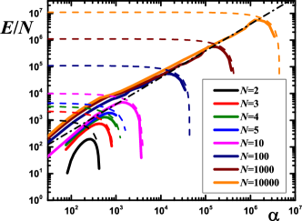
Figure 10: (Color online) The energy per particle in the many-body system for the soft-sphere interaction potential, as a function of the inverse-Gaussian-width parameter, $\alpha$ (see Eq. (84)), for $U_{0}=1$, $a_{s}=0.1$, $R=1.3a_{s}$ and the number of particles $N=2,3,4,5,10,100,1000,10000$ (larger numbers of particles have a larger value at the maximum), as obtained in Ref. GEA . Solid lines: the variational result; dashed lines: the asymptotic energy of the fully-collapsed state, as per Eq. (96); the dash-dotted line: typical energy associated with the Gaussian localization, as given by Eq. (95).

For large $N$, the energy calculated with ansatz (84) does not immediately lead to the fully collapsed state. The localization energy, proportional to the energy scale, $\hbar\Omega$, of the trapping potential, may become a dominating term in the energy, while the system’s size is still large enough, so that the fully-collapsed state is not realized. The energy in the corresponding regime is numerically approximated as

$$E=NC\alpha$$ (95)

with $C=4$. It is shown in Fig. 10 by the dashed-dotted line. For still tighter localization, it has been found that, in the limit of the full collapse, when all particles overlap, the energy is well approximated by formula

$$E=NE^{(1)}+N(N-1)V_{0}.$$ (96)

The energy of the interparticle interactions, revealed by the calculations, is $E_{\mathrm{int}}=V_{0}N(N-1)/2$. The asymptotic energy (96) is shown in Fig. 3 by dashed lines.

A clear conclusion is that the increase of the number of particles indeed causes strong rise of the potential barrier which stabilizes the metastable energy minimum corresponding to the gaseous state. This can be also concluded from Eq. (96), where the contribution due to the repulsive interactions scales as $N^{2}$ for large $N$, while the term corresponding the attractive central potential scales as $N$.

The energy barrier between the state described by ansatz (84) and the free state with zero energy, $E_{\mathrm{barrier}}$, is estimated as the maximum value of the energy per particle (see Fig. 3), and is shown in Fig. 4. For a large system’s size, the barrier can be approximated by comparing the two basic energy scales given by Eqs. (95) and (96). The resulting asymptotic approximation for the barrier’s height is

$$E_{\mathrm{barrier}}=6NV_{0}/(8U_{0}-3+2C),$$ (97)

which is shown in Fig. 4 by the dashed line.

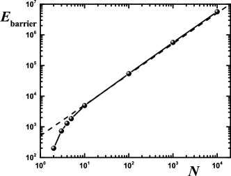
Figure 11: The energy barrier between the state with $\alpha=0$ and $\alpha\rightarrow\infty$ in the many-body system, as a function of the number of particles, $N$, for the data shown in Fig. 10, as per Ref. GEA . The dashed line depicts the asymptotic approximation (97) for the large system.

VI Discussion and conclusion

This article aims to produce a brief review of results reported in works HS1 -HS3 and GEA , that offer a solution to the known problem of the quantum collapse, alias “fall onto the center” LL , in nonrelativistic quantum mechanics. The quantum collapse occurs in the three-dimensional Schrödinger equation with 3D isotropic attractive potential $-U_{0}/(2r^{2})$. This equation does not have a GS (ground state) if the attraction strength, $U_{0}$, exceeds a final critical value. In that case, the Schrödinger equation gives rise to a nonstationary wave function which collapses, shrinking towards the center. The solution of the collapse problem was proposed in the above-mentioned original works in terms of the gas of bosons pulled to the center by the same potential, with repulsive contact interactions between the particles. The intrinsic repulsion is represented by the cubic term in the respective GPE (Gross-Pitaevskii equation). The setting may be realized as the 3D gas of polar molecules carrying a permanent electric dipole moment and pulled to a central electric charge. The analysis, performed in the framework of the mean-field theory, predicts suppression of the collapse in the gas, and the creation of the missing GS.

An original result, added in this article to the review of the previously published findings, is the quantum phase transition occurring in the 3D model which includes the beyond-mean-field LHY (Lee-Huang-Yang) correction in the GPE, in the form of the self-repulsive quartic term. The phase transition manifests itself by a jump of the asymptotic structure of the wave function (for $r\rightarrow 0$) at the critical value of the strength of the attractive potential.

In the 2D version of the model, the cubic self-repulsion is not sufficient to suppress the quantum collapse. In this case, it can be suppressed if a quintic self-repulsive term, representing three-body collisions (provided that they so not give rise to losses) can be added to the underlying GPE. On the other hand, the LHY quartic term, added to the 2D GPE, is sufficient to suppress the quantum collapse and restore the respective GS.

Polarization of dipole moments in the 3D gas by an external uniform field reduces the symmetry of the central attractive potential from spherical to cylindrical. This modification of the system predicts both the GS and stabilized states carrying the angular momentum. A binary condensate, modelled by the system of nonlinearly-coupled GPEs, is considered too, making it possible to study the interplay of the suppression of the collapse in the 3D space and the miscibility-immiscibility transition in the binary BEC.

In addition to the systematic numerical analysis of these mean-field settings, the original works have produced many results by means of analytical approximations, such as combined asymptotic expansions and TFA (Thomas-Fermi approximation). All the states predicted by the mean-field theory in these settings are shown to be completely stable as solutions to the respective time-depending GPEs.

In work GEA , the consideration of the same 3D setting was performed in terms of the many-body quantum theory, by means of the variational approximation for the many-body wave function, numerically handled with the help of the Monte-Carlo method. The analysis has demonstrated that, although the quantum collapse cannot be fully suppressed in terms of the many-body theory, the self-trapped states predicted by the mean-field model exist in the full many-body setting too, as metastable ones, protected against the onset of the collapse by a tall potential barrier, whose height steeply grows with the increase of the number of particles in the gas.

As an extension of the work on the topic of this article, it may be interesting to construct modes carrying the angular momentum in the isotropic 3D model, and also to consider the model with a set of two mutually symmetric attractive centers. In particular, it may be relevant to explore a possibility of the spontaneous symmetry breaking of the GS in the latter case.

As mentioned above (see Eqs. (43) and (44), a challenging issue is to develop a consistent analysis for the gas of fermions pulled to the center by the same potential, $\ -U_{0}/\left(2r^{2}\right)$.

Conflict of interests

The author declares no conflict of interest in the context of this paper.

References

- (1) Landau, L. D.; Lifshitz, E. M. Quantum Mechanics: Nonrelativistic Theory. Nauka publishers: Moscow, USSR, 1974.
- (2) Gupta, K. S.; Rajeev, S. G. Renormalization in quantum mechanics. Phys. Rev. D 1993, 48, 5940-5945.
- (3) Camblong, H. E.; Epele, L. N.; Fanchiotti, H.; García Canal, C. A. Renormalization of the Inverse Square Potential. Phys. Rev. Lett. 2000, 85, 1590.
- (4) Ávila-Aoki, M.; Cisneros C.; Martínez-y-Romero, R. P.; Núñez-Yepez, H. N.; Salas-Brito, A. L. Classical and quantum motion in an inverse square potential. Phys. Lett. A 373, 418-421 (2009).
- (5) Sakaguchi, H.; Malomed, B. A. Suppression of the quantum-mechanical collapse by repulsive interactions in a quantum gas. Phys. Rev. A 2011, 83, 013607.
- (6) Sakaguchi, H.; Malomed, B. A. Suppression of the quantum collapse in an anisotropic gas of dipolar bosons. Phys. Rev. A 2011, 84, 033616.
- (7) Sakaguchi, H.; Malomed, B. A. Suppression of the quantum collapse in binary bosonic gases. Phys. Rev. A 2013, 88, 043638).
- (8) Pitaevskii, L. and Stringari, S. Bose-Einstein Condensation. Clarendon: Oxford, UK, 2003.
- (9) Schmid, S.; Härter, A.; Denschlag, J. H. Dynamics of a cold trapped Ion in a Bose-Einstein condensate. Phys. Rev. Lett. 2010, 105, 133202.
- (10) Deiglmayr, J.; Grochola, A.; Repp, M.; Mörtlbauer, K.; Glück, C.; Lange, J.; Dulieu, O.; Wester, R.; Weidemüller M. Formation of ultracold polar molecules in the rovibrational ground state. Phys. Rev. Lett. 2008, 101, 133004.
- (11) Ospelkaus, S.; Ni, K.-K.; Quéméner, G.; Neyenhuis, B.; Wang, D.; de Miranda, M. H. G.; Bohn, J. L.; Ye, J.; Jin, D. S. Controlling the hyperfine state of rovibronic ground-state polar molecules. Phys. Rev. Lett. 2010, 104, 030402.
- (12) Posazhennikova, A. Colloquium: Weakly interacting, dilute Bose gases in 2D. Rev. Mod. Phys. 2006, 78, 1111-1134.
- (13) Denschlag, J.; Schmiedmayer, J. Scattering a neutral atom from a charged wire. Europhys. Lett. 1997, 38, 405-410.
- (14) Olshanii, M.; Perrin, H.; Lorent, V. Example of a quantum anomaly in the physics of ultracold gases. Phys. Rev. Lett. 2010, 105, 095302.
- (15) Sakaguchi, H.; Malomed, B. A. Solitons in combined linear and nonlinear lattice potentials. Phys. Rev. A 2010, 81, 013624.
- (16) Vakhitov, M.; Kolokolov, A. Stationary solutions of the wave equation in a medium with nonlinearity saturation. Radiophys. Quantum Electron. 1973, 16, 783-789.
- (17) Bergé, L. Wave collapse in physics: principles and applications to light and plasma waves. Phys. Rep. 1998, 303, 259-370.
- (18) Dodd, R. J. Approximate solutions of the nonlinear Schrödinger equation for ground and excited states of Bose-Einstein condensates. J. Res. Natl. Inst. Stand. Technol. 1996, 101, 545-552.
- (19) Dalfovo, F., Stringari, S. Bosons in anisotropic traps: Ground state and vortices. Phys. Rev. A 1996, 53, 2477-2485.
- (20) Alexander, T. J., Bergé, L. Ground states and vortices of matter-wave condensates and optical guided waves. Phys. Rev. E 2002, 65, 026611.
- (21) Malomed, B. A., Lederer, F., Mazilu, D., Mihalache, D. On stability of vortices in three-dimensional self-attractive Bose-Einstein condensates. Phys. Lett. A 2007, 361, 336-340.
- (22) Lee, T. D.; Huang, K.; Yang, C. N. Eigenvalues and eigenfunctions of a Bose system of hard spheres and its low-temperature properties. Phys. Rev. 1957, 106, 1135-1145.
- (23) Petrov, D. S. Quantum mechanical stabilization of a collapsing Bose-Bose mixture. Phys. Rev. Lett. 2015, 115, 155302.
- (24) Petrov, D. S.; Astrakharchik, G. E. Ultradilute low-dimensional liquids, Phys. Rev. Lett. 2016, 117, 100401.
- (25) Astrakharchik, G. E.; Gangardt, D. M.; Lozovik, Yu. E.; Sorokin, I. A. Off-diagonal correlations of the Calogero-Sutherland model, Phys. Rev. E 2006, 74, 021105.
- (26) Chubukov, A. V.; Pépin, C.; Rech, J. Instability of the quantum-critical point of itinerant ferromagnets, Phys. Rev. Lett. 2004, 92, 147003.
- (27) de Oliveira, T. R.; Rigolin, G.; de Oliveira, M. C.; Miranda, E. Multipartite entanglement signature of quantum phase transitions. Phys. Rev. Lett. 2007, 97, 170401.
- (28) Mazzanti, F.; Astrakharchik, G. E.; Boronat, J.; Casulleras, Off-diagonal ground-state properties of a one-dimensional gas of Fermi hard rods. J. Phys. Rev. A 2008, 77, 043632.
- (29) Zhao, J.-H.; Zhou, H.-Q. Singularities in ground-state fidelity and quantum phase transitions for the Kitaev model. Phys. Rev. B 2009, 80, 014403.
- (30) Yao, Y.; Li, H. W.; Zhang, C.-M.; Yin, Z. Q.; Chen, W. C.; Guo, G.-C.; Han Z.-F. Performance of various correlation measures in quantum phase transitions using the quantum renormalization-group method. Phys. Rev. A 2012, 86, 042102.
- (31) Cabrera, C. R., Tanzi, L., Sanz, J., Naylor, B., Thomas, P., Cheiney, P., Tarruell, L. Quantum liquid droplets in a mixture of Bose-Einstein condensates. Science 2018, 359, 301-304.
- (32) Cheiney, P., Cabrera, C. R., Sanz, J., Naylor, B., Tanzi, L., Tarruell, L. Bright soliton to quantum droplet transition in a mixture of Bose-Einstein condensates. Phys. Rev. Lett. 2018, 120, 135301.
- (33) Semeghini, G., Ferioli, G., Masi, L., Mazzinghi, C., Wolswijk, L., Minardi, F., Modugno, M., Modugno, G., Inguscio, M., Fattori, M. Self-bound quantum droplets in atomic mixtures. arXiv:1710.10890.
- (34) Abdullaev, F. Kh.; Gammal, A., Tomio, L.; Frederico, T. Stability of trapped Bose-Einstein condensates. Phys. Rev. A 2001, 63, 043604.
- (35) Abdullaev, F. Kh.; Salerno, M. Gap-Townes solitons and localized excitations in low-dimensional Bose-Einstein condensates in optical lattices. Phys. Rev. A 2005, 72, 033617.
- (36) Petrov, D. S., Holzmann, M., Shlyapnikov G. V. Bose-Einstein condensation in quasi-2D trapped gases. Phys. Rev. Lett. 2000, 84, 2551-2555.
- (37) Salasnich, L., Parola, A., Reatto, L. Effective wave equations for the dynamics of cigar-shaped and disk-shaped Bose condensates. Phys. Rev. A 2002, 65, 043614.
- (38) Muñoz Mateo, A., Delgado, V. Effective mean-field equations for cigar-shaped and disk-shaped Bose-Einstein condensates. Phys. Rev. A 2008, 77, 013617.
- (39) Giorgini, S.; Pitaevskii, L. P.; Stringari, S. Theory of ultracold atomic Fermi gases. Rev. Mod. Phys. 2008, 80, 1215-1273.
- (40) Capuzzi, P.; Minguzzi, A.; Tosi, M. P. Collective excitations of a trapped boson-fermion mixture across demixing. Phys. Rev. A 2003, 67, 053695.
- (41) Adhikari, S. K. Fermionic bright soliton in a boson-fermion mixture. Phys. Rev. A 2005, 72, 053608.
- (42) Manini, N.; Salasnich, L. Bulk and collective properties of a dilute Fermi gas in the BCS-BEC crossover. Phys. Rev. A 2005, 71, 033625.
- (43) Bulgac, A.; Local-density-functional theory for superfluid fermionic systems: The unitary gas. Phys. Rev. A 2007, 76, 040502(R).
- (44) Góral, K.; Santos, L. Phys. Rev. A 2002, 66, 023613.
- (45) Deconinck, B.; Kevrekidis, P. G., Nistazakis, H. E.; Frantzeskakis, D. J. Linearly coupled Bose-Einstein condensates: From Rabi oscillations and quasiperiodic solutions to oscillating domain walls and spiral waves, Phys. Rev. A 2004, 70, 063605.
- (46) Adhikari, S. K.; Malomed, B. A. Two-component gap solitons with linear interconversion. Phys. Rev. A 2009,79, 015602.
- (47) Wen, L.; Liu, W. M.; Cai, Y.; Zhang, J. M.; Hum J. Controlling phase separation of a two-component Bose-Einstein condensate by confinement. Phys. Rev. A 2012, 85, 043602.
- (48) Mineev, V. P. Theory of solution of two almost perfect Bose gases, Zh. Eksp. Teor. Fiz. 1974, 67, 263-272 [Sov. Phys. JETP 1975, 40, 132].
- (49) Wang, J.; Cerdeiriña, C. A.; Anisimov, M. A.; Sengers, J. V. Principle of isomorphism and complete scaling for binary-fluid criticality. Phys. Rev. E 2008, 77, 031127.
- (50) Roeksabutr, A.; Mayteevarunyoo, T.; Malomed, B. A. Symbiotic two-component gap solitons. Opt. Exp. 2012, 20, 24559-24574.
- (51) Astrakharchik, G. E.; Malomed, B. A. Quantum versus mean-field collapse in a many-body system, Phys. Rev. A 2015, 92, 043632.
- (52) Metropolis, N.; Rosenbluth, A. W.; Rosenbluth, M. N.; Teller, A. H. Equation of state calculations by fast computing machines. J. Chem. Phys. 1953, 21, 1087.
- (53) Jastrow, R. Many-body problem with strong forces. Phys. Rev. 1955, 98, 1479-1484.