Instantaneous ionization rate as a functional derivative.

Abstract

We describe an approach defining instantaneous ionization rate (IIR) as a functional derivative of the total ionization probability. The definition is based on physical quantities which are directly measurable, such as the total ionization probability and the waveform of an ionizing pulse. The definition is, therefore, unambiguous and does not suffer from gauge non-invariance. We compute IIR by solving numerically the time-dependent Schrödinger equation for the hydrogen atom in a strong laser field. In agreement with some previous results using attoclock methodology, the IIR we define does not show measurable delay in strong field tunnel ionization.

The notion of the instantaneous ionization rate (IIR) proved extremely fruitful for understanding physics of tunelling ionization, the ionization regime characterized by small values of the Keldysh parameter $\gamma=\omega/E_{0}\sqrt{2|I|}\lesssim 1$ Keldysh (1965); Krausz and Ivanov (2009) (here $\omega$, $E_{0}$ and $I$ are the frequency, field strength and ionization potential of a target system expressed in atomic units).

Qualitatively, the fact that the IIR is a function which is sharply peaked near the local maxima of the electric field of the pulse, can be used to pinpoint the most probable electron trajectory. This provides a basis for the design and interpretation of the results of well-known experimental techniques, such as attosecond streaking, or angular attosecond streaking Itatani et al. (2002); Baltuška et al. (2003); Eckle et al. (2008) allowing to follow electron dynamics at the attosecond level of precision. Recently, the temporarily localized ionization at the local maxima of the laser field has been used as a fast temporal gate to measure the laser field Park et al. (2018).

Quantitatively, the notion of IIR underlies many successful simulations of tunneling ionization phenomena, relying on classical (CTMC method) Shvetsov-Shilovski et al. (2012) or quantum trajectories (QTMC) Li et al. (2014); Shvetsov-Shilovski et al. (2016) Monte-Carlo simulations. These methods become practically indispensable if the system in question is too complicated to allow an ab initio treatment based on the numerical solution of the time-dependent Schrödinger equation (TDSE). Even if numerical solution of the TDSE is possible, these methods may provide physical insight which is not obvious from the TDSE wave-function. Accurate quantitative calculations using these approaches, which agree well with the ab initio TDSE have been reported in the literature Shvetsov-Shilovski et al. (2012); Hofmann et al. (2013); Pfeiffer et al. (2012); Arbo et al. (2015); Dimitrovski and Madsen (2015); Landsman and Keller (2015); Hofmann et al. (2016). In these approaches the quantum-mechanical Keldysh-type theories Keldysh (1965); Faisal (1973); Reiss (1980); Perelomov et al. (1966) are used to set up initial conditions for the subsequent electron motion Pfeiffer et al. (2012); Arbo et al. (2015); Dimitrovski and Madsen (2015). IIR in the well-known ADK form Ammosov et al. (1986); Delone and Krainov (1991), or more refined Yudin-Ivanov IIR Yudin and Ivanov (2001) provides a measure allowing to assign probability to an ionization event occurring at a given moment of time inside the laser pulse duration.

The notion of the ionization event occurring at a given time and, correspondingly, the notion of IIR are not free from certain ambiguity, however. An interpretation of the ionization event which is often used is based on the imaginary time method Perelomov et al. (1966); Popruzhenko (2014). In this picture an electron enters the tunelling barrier at some complex moment of time with complex velocity. Upon descending on the real axis, the velocity and coordinates corresponding to the most probable electron trajectory become real, which can be interpreted as the electron’s exit from under the barrier. This picture, however, cannot be taken unreservedly, since the path which descends on the real axis is not unique and can be deformed, in principle, to cross the real time-axis at almost any given point Popruzhenko (2014). An approach allowing to define IIR from the solution of the TDSE has been described recently Yuan et al. (2017). In this approach the IIR is defined by projecting out contributions of the bound states from the solution of the TDSE. The authors found that the IIR thus defined lags behind the local maxima of the electric field, which suggests a non-zero tunneling time. A shortcoming of this definition of the IIR, however, is its non-gauge-invariant character. The projection of the solution of the TDSE on the subspace of the bound states performed during the interval of the pulse duration depends generally on the gauge used to describe atom-field interaction. Another approach allowing to define IIR from the solution of the TDSE based on the notion of the electron flux was given in Teeny et al. (2016).

In the present work we describe a novel approach to IIR, which is based on the notion of a functional derivative. Total ionization probability can be considered as a functional $P[E]$ of the waveform $E(t)$, which maps the electric field of the pulse into a real number. For the regime of the tunneling ionization we are interested in below, this functional is highly non-linear and cannot be described in a closed form. A simplification is possible if we consider a waveform which can be represented as $E(t)=E_{f}(t)+\delta E(t)$, with fundamental field $E_{f}(t)$ and signal field $\delta E(t)$. To be more specific, let us assume that the fundamental field is linearly polarized (along $z-$ axis) and is defined by the vector potential ${\bm{A}_{f}(t)}$:

$${\bm{A}_{f}(t)}=-\hat{\bm{z}}{E_{0}\over\omega}\sin^{2}{\left\{\pi t\over T_{1}\right\}}\sin{\omega t}\ ,$$ (1)

with peak field strength $E_{0}$, carrier frequency $\omega$, and total duration $T_{1}=NT$, where $T=2\pi/\omega$ is an optical period (o.c.) corresponding to the carrier frequency $\omega$, with $N\in\mathbb{N}$.

We assume the signal field to vanish outside the interval $(0,T_{1})$ of the fundamental pulse duration. If the signal field $\delta E(t)$ is sufficiently weak we can write:

$$\delta P=P[E_{f}+\delta E]-P[E_{f}]\approx\int\limits_{0}^{T_{1}}{\delta P\over\delta E_{f}(t)}\delta E(t)dt\ ,$$ (2)

where $\displaystyle{\delta P\over\delta E_{f}(t)}$ is a functional derivative of the functional $P[E]$ evaluated for $E(t)=E_{f}(t)$.

On the other hand, using the customary definition of IIR, we can write for the probability of ionization driven by the combined field $E(t)=E_{f}(t)+\delta E(t)$:

$$P_{\rm inst}=\int\limits_{0}^{T_{1}}W_{\rm inst}(E(t))\ dt\ ,$$ (3)

where $W_{\rm inst}(E(t))$ is the IIR, which by definition depends on the instantaneous value $E(t)$ of the electric field. We introduced the notation $P_{\rm inst}$ in Eq. (3) to emphasize that this expression pertains to the notion of the IIR. Eq. (3) gives a very particular case of the functional $P[E]$ – clearly not every functional can be represented in this way.

From Eq. (3) we obtain the change of the ionization probability $P_{\rm inst}$ due to the presence of the weak signal field:

$$\delta P_{\rm inst}\approx\int\limits_{0}^{T_{1}}{dW_{\rm inst}(E_{f}(t))\over dE(t)}\delta E(t)dt\ ,$$ (4)

Taking into account that $\delta E(t)$ in Eq. (2) and Eq. (4) is arbitrary (provided it is small and vanishes outside the interval $(0,T_{1})$), one can see that, if the treatment based on the notion of the IIR is justified (i.e. using Eq. (3) with IIR $W_{\rm inst}(E(t))$ depending only on the instantaneous value of the electric field one obtains accurate value for the total ionization probability), one must have:

$${\delta P\over\delta E_{f}(t)}\approx{dW_{\rm inst}(E_{f}(t))\over dE(t)}\ .$$ (5)

We note that the quantity on the r.h.s of (5) is an ordinary derivative which depends on time only through the instantaneous value of the electric field. The quantity on the l.h.s., on the other hand, is a functional derivative, which depends on time (through the time moment $t$ at which differentiation is performed), and on the waveform $E(t)$, i.e., on the complete history, past and future, of the pulse. Suppose, for instance, that we represent the waveform (1) as a Fourier series:

$$E(t)=\sum\limits_{m}a_{m}e^{im\Omega t}\ ,$$ (6)

where $\Omega=2\pi/T_{1}$. In general, the functional derivative on the l.h.s. of Eq. (5) depends on the whole set ${a_{m}}$, while the ordinary derivative on the r.h.s. is a function of the particular combination of these coefficients. To express this differently, suppose, that we fix the pulse shape in Eq. (1) and allow only the field amplitude $E_{0}$ to vary. The l.h.s of Eq. (5) would then generally be a function of two variables $E_{0}$ and $t$, while the r.h.s. would depend only on a particular combination of $E_{0}$ and $t$ which gives the instantaneous field strength $E(t)$. Exact equality in Eq. (5), therefore, cannot be achieved in general. This clearly demonstrates the approximative character of the notion of the IIR. The more accurate expression (2), based on the functional derivative of the ionization probability functional, depends not only on time, but on additional variables describing the waveform as well. For brevity, we will dub below the functional derivative in Eq. (2) an ”exact ionization rate”, though as one can see from Eq. (5), it rather corresponds to the derivative of the IIR with respect to the electric field.

To compute the exact ionization rate in Eq. (5) for a given moment of time $\tau$ and a given waveform $E_{f}(t)$, one can calculate numerically the modulation of the ionization probability $\delta P$ using $E_{f}(t)$ as a fundamental field and employing a special form $\delta E(t,\tau)=\alpha\delta(t-\tau)$ of the signal field, containing the Dirac delta-function. We did this by solving numerically the TDSE for a hydrogen atom in the presence of the pulse (1). We considered pulses with the low carrier frequency of $\omega=0.02$ a.u. We need to work with low frequencies to stay within the framework of the adiabatic theory, which makes the notion of the instantaneous ionization rate at least qualitatively applicable. We report below results of the calculations with total pulse durations $T_{1}$ of one or two optical cycles respectively, and various peak field strengths $E_{0}$ (chosen such as to remain in the tunelling regime of ionization).

The solution of the TDSE has been found by representing the wave function as a series in spherical harmonic functions, and discretizing the resulting system of radial equations on a grid with the step-size $\delta r=0.05$ a.u. in a box of the size $R_{\rm max}=700$ a.u., which was sufficient for the pulses of a short duration we consider below. More details about the numerical procedure used to solve the TDSE can be found in Refs. Ivanov (2014); Ivanov and Kheifets (2013).

Total ionization probability, which we need for the practical implementation of the definition (5), is found by decomposing the wave function at the end of the pulse as:

$$\Psi(T_{1})=\phi+\chi,$$ (7)

where $\phi=\hat{Q}\Psi(T_{1})$, $\chi=(\hat{I}-\hat{Q})\Psi(T_{1})$ , and $\hat{Q}$ is the projection operator on the subspace of the bound states of the field-free atomic Hamiltonian. Total ionization probability $P$ can be found then as the squared norm $P=||\chi||^{2}$. Projection operator $\hat{Q}$ is obtained by computing numerically (employing the same grid we used to solve the TDSE) the bound states $|nl\rangle$ of the field-free Hamiltonian:

$$\hat{Q}=\sum\limits_{nl\atop l=0}^{L_{b}}|nl\rangle\langle nl|\ ,$$ (8)

where we retain all eigenvectors we obtain $0\leq l\leq L_{b}$. We used $L_{b}=12$ in the calculations below (having checked that results are well converged with respect to this parameter). We note that definition of the ionization probability as the squared norm of $\chi$ is formally equivalent to the often used definition in terms of the projection on the asymptotic scattering states $\phi_{{\bm{k}}}$: $\displaystyle P=\int d{\bm{k}}|\langle\phi_{{\bm{k}}}|\Psi(T_{1})\rangle|^{2}$ (assuming normalization $\langle\phi_{{\bm{k}}^{\prime}}|\phi_{{\bm{k}}}\rangle=\delta({\bm{k}}-{\bm{k}}^{\prime})$). Indeed, substituting decomposition (7) in this equation, and using orthogonality of $\chi$ to the subspace of the bound states, we obtain again $P=||\chi||^{2}$. In practice, the prescription $P=||\chi||^{2}$, we use in the calculations below, is preferable. The reason for this is that calculation of the total ionization probability by projecting $\Psi(T_{1})$ on the set of the scattering states implicitly presumes the strict orthogonality of the scattering and bound atomic states. We are interested below not in the ionization probability itself, but rather in its relatively small variations due to the weak signal field. Even small non-orthogonality of the scattering and bound states unavoidable in numerical calculations may lead to a significant loss of precision.

The definition of exact ionization rate in Eq. (2) is based on the physically observable quantities: the electric field of the pulse and modulation of the total ionization probability. It is clearly gauge invariant. It is immaterial, therefore, which gauge describing the atom-field interaction is used when solving the TDSE (provided, of course, that a sufficient level of numerical accuracy has been achieved). We used the length (L-) gauge. Convergence of the expansions in spherical harmonic functions we use to represent the solution of the TDSE was achieved by including spherical harmonic functions of the rank up to $L_{\rm max}=70$. In numerical calculations we have to regularize, of course, the expression $\delta E(t,\tau)=\alpha\delta(t-\tau)$ for the signal field. We used the regularization:

$$\delta E(t,\tau)={\alpha\over\epsilon}\exp\left\{-{(t-\tau)^{2}\over\epsilon^{2}}\right\}\ ,$$ (9)

with $\epsilon=T/1000$ (here $T$ is an optical period corresponding to the carrier frequency we use), and $\alpha=0.001$. The value of $\alpha$ is to be chosen so that the higher order functional derivatives in the Taylor expansion for the the ionization probability functional in Eq. (2) can be omitted. That our choice of this parameter warrants such an omission is shown in the Supplemental Material, which presents a detailed study of the influence of the parameters $\alpha$ and $\epsilon$ on the accuracy of the calculation. It is worth noting that even for $\epsilon=T/30$ the relative error we get for the ionization probability is of the order of one percent. FWHM of the pulse (9) for this value of $\epsilon$ is about $300$ attoseconds. Delta-function-like pulses of such duration have already been produced in the laboratory Hassan et al. (2016), which makes possible experimental measurements of the IIR which we define in the present work.

We will fix below the functional form of the fundamental pulse shape in Eq. (1) and allow only the peak field strength $E_{0}$ of the fundamental field to vary. In figures below we show and analyze not the functional derivative itself but a proportional quantity: the first variation of the ionization probability $\delta P(E_{0},\tau)$, obtained if we substitute expression (9) for the signal field in Eq. (2).

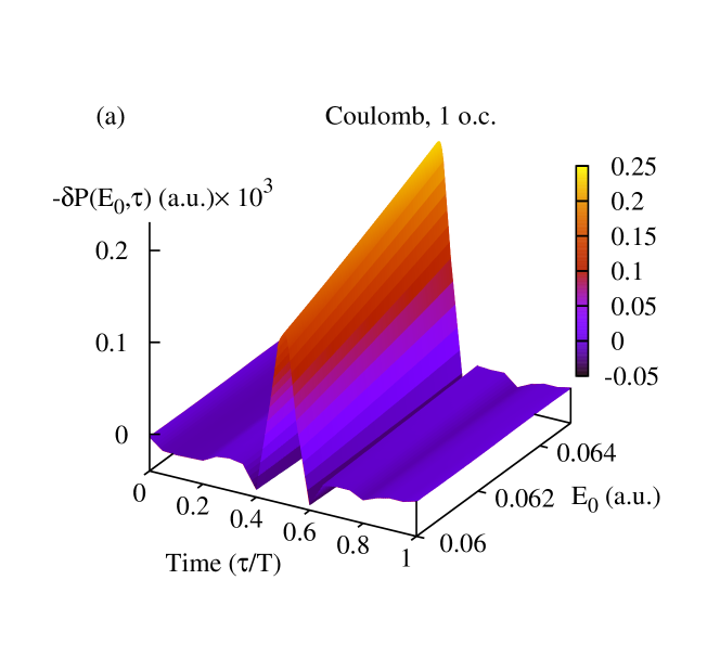
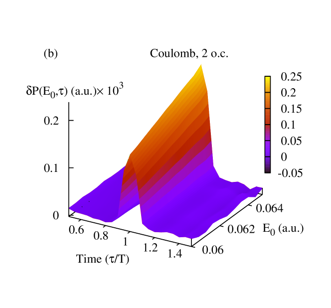
Figure 1: (Color online) First variation of the ionization probability $\delta P(E_{0},\tau)$ obtained from TDSE for Coulomb potential for the total pulse duration of 1 o.c. (a) and 2.o.c (b).

We show in Figure 1 the first variation $\delta P(E_{0},\tau)$ computed following the numerical procedure outlined above as a function of time $\tau$ and electric field strength $E_{0}$ for the pulses (1) with total duration $T_{1}$ of one or two optical cycles.

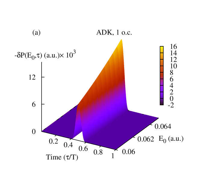
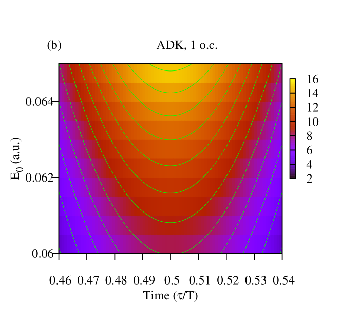
Figure 2: (Color online) First variation of the ionization probability $\delta P(E_{0},\tau)$ obtained for ADK IIR for the total pulse duration of 1 o.c. (a). Contour plot of $\delta P(E_{0},\tau)$ (b).

In Fig.2a we present $\delta P(E_{0},\tau)$ obtained using the ADK expression Ammosov et al. (1986); Delone and Krainov (1991) for the IIR. Since the ADK ionization probability assumes an instantaneous relation between the field strength and the probability of ionization at any given time, this naturally leads to a definition of the IIR following equation Eq. (4).

More detailed picture of the IIR’s emerges by looking at the contour plots (i.e. lines of equal elevation) of $\delta P(E_{0},\tau)$ in the $E_{0},\tau$-plane. Of particular interest is, of course, the behavior of the IIR near the local maxima of the electric field where the IIR attains its largest values. We will concentrate, therefore, on the region of $\tau$-values close to the highest maximum of the electric field strength. We will consider below only the pulses with a total duration of one o.c., the results for the pulses with duration of 2 o.c. have been found to be essentially the same as for 1 o.c. duration.

Since the ADK IIR is a function of the instantaneous electric field only, lines of constant elevation in this case are just the lines satisfying $|E(\tau)|={\rm const}$. Contour lines given by this equation are shown in Fig. 2b. The curves are perfectly symmetric with respect to the instant of time when electric field of the pulse has a maximum, and are parabolic near this point. These features, of course, can be readily deduced from the fact that the electric field of the pulse (1) is an even function, symmetric about the midpoint of the pulse.

Any asymmetry of the contour lines about the midpoint of the pulse could be interpreted as a manifestation of the tunneling delay, as was done in Yuan et al. (2017), where a lag was found for the IIR defined in that work by projecting out bound states contributions from the TDSE wave-function. Or in Teeny et al. (2016), where the authors monitored the probability current density at the (albeit adiabatic) exit point, as calculated by a one-dimensional TDSE solution. The point of view that the tunneling delay has a non-zero value has also been expressed in the works Teeny et al. (2016); Zimmermann et al. (2016); Landsman et al. (2014); Douguet and Bartschat (2018); Camus et al. (2017), as opposed to the papers advocating view of tunelling as an instantaneous process Torlina et al. (2015); Ni et al. (2016, 2018). Fig. 3a shows contour lines of $\delta P(E_{0},\tau)$ obtained from TDSE calculation for hydrogen with the Coulomb potential. The absence of any appreciable asymmetry in the Figure suggests that our definition of the IIR gives us an essentially zero time delay for the Coulomb potential.

We considered also the case of the Yukawa potentials $V(r)=-A{\bm{e}}^{-{r\over a}}/r$ with different screening parameters $a$. For every $a$ we adjusted the value of $A$ so that the resulting ionization potential for the ground state was always $0.5$ a.u., corresponding to hydrogen. Results for the Yukawa potentials shown in Fig 3b, Fig.3c again show an absence of any appreciable asymmetry of the contour lines, and consequently the time delay.

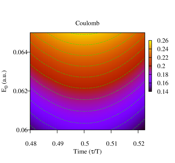
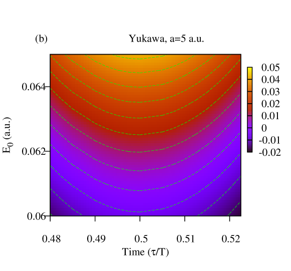
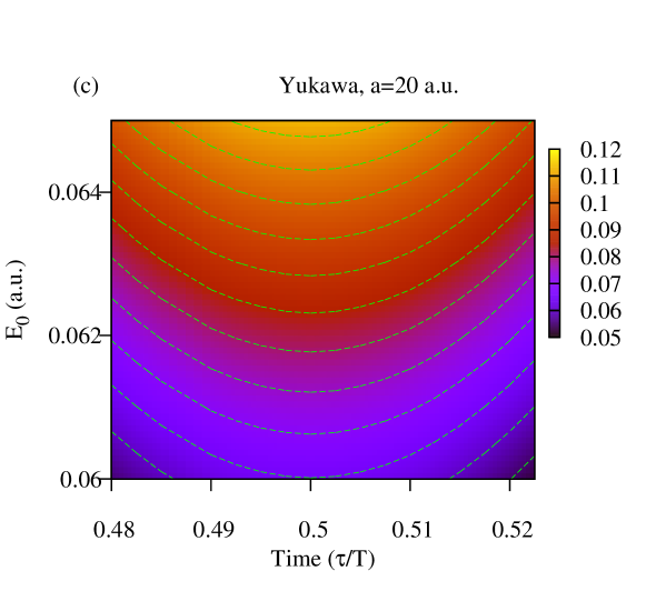
Figure 3: (Color online) Contour plots of $\delta P(E_{0},\tau)$ for the Coulomb potential (a) and Yukawa potentials with different screening parameters (b),(c).

To summarize, we described an approach allowing to define the IIR as a functional derivative of the total ionization probability. This approach provides an unambiguous definition of the IIR. In particular, it is based on directly measurable quantities, such as the total ionization probability and the waveform of the pulse, which makes it gauge invariant. We studied the IIR thus defined using tunneling ionization of systems with Coulomb and Yukawa potentials as examples. In agreement with some previous results using attoclock methodology (which assume the most probable electron trajectory to begin tunneling at the peak of the laser field), the IIR we define does not show any appreciable tunelling delay in strong field ionization for the case of hydrogen.

References

- Keldysh (1965) L. V. Keldysh, Sov. Phys. -JETP 20, 1307 (1965).
- Krausz and Ivanov (2009) F. Krausz and M. Ivanov, Rev. Mod. Phys. 81, 163 (2009).
- Itatani et al. (2002) J. Itatani, F. Quéré, G. L. Yudin, M. Y. Ivanov, F. Krausz, and P. B. Corkum, Phys. Rev. Lett. 88, 173903 (2002).
- Baltuška et al. (2003) A. Baltuška, T. Udem, M. Uiberacker, M. Hentschel, E. Goulielmakis, C. Gohle, R. Holzwarth, V. S. Yakovlev, A. Scrinzi, T. W. Hänsch, et al., Nature 421, 611 (2003).
- Eckle et al. (2008) P. Eckle, A. N. Pfeiffer, C. Cirelli, A. Staudte, R. Dörner, H. G. Muller, M. Büttiker, and U. Keller, Science 322, 1525 (2008).
- Park et al. (2018) S. B. Park, K. Kim, W. Cho, S. Hwang, I. Ivanov, C.H.Nam, and K.T.Kim, Optica 5, 402 (2018).
- Shvetsov-Shilovski et al. (2012) N. I. Shvetsov-Shilovski, D. Dimitrovski, and L. B. Madsen, Phys. Rev. A 85, 023428 (2012).
- Li et al. (2014) M. Li, J.-W. Geng, H. Liu, Y. Deng, C. Wu, L.-Y. Peng, Q. Gong, and Y. Liu, Phys. Rev. Lett. 112, 113002 (2014).
- Shvetsov-Shilovski et al. (2016) N. I. Shvetsov-Shilovski, M. Lein, L. B. Madsen, E. Räsänen, C. Lemell, J. Burgdörfer, D. G. Arbó, and K. TH2 okési, Phys. Rev. A 94, 013415 (2016).
- Hofmann et al. (2013) C. Hofmann, A. Landsman, C. Cirelli, A. Pfeiffer, and U. Keller, J. Phys. B 46, 125601 (2013).
- Pfeiffer et al. (2012) A. N. Pfeiffer, C. Cirelli, A. S. Landsman, M. Smolarski, D. Dimitrovski, L. B. Madsen, and U. Keller, Phys. Rev. Lett. 109, 083002 (2012).
- Arbo et al. (2015) D. G. Arbo, C. Lemell, S. Nagele, N. Camus, L. Fechner, A. Krupp, T. Pfeifer, S. D. Lopez, R. Moshammer, and J. Burgdorfer, Phys. Rev. A 92, 023402 (2015).
- Dimitrovski and Madsen (2015) D. Dimitrovski and L. B. Madsen, Phys. Rev. A 91, 033409 (2015).
- Landsman and Keller (2015) A. S. Landsman and U. Keller, Physics Reports 547, 1 (2015).
- Hofmann et al. (2016) C. Hofmann, T. Zimmermann, A. Ziellinski, and A. Landsman, New Journal of Physics 18, 043011 (2016).
- Faisal (1973) F. H. M. Faisal, J. Phys. B 6, L89 (1973).
- Reiss (1980) H. R. Reiss, Phys. Rev. A 22, 1786 (1980).
- Perelomov et al. (1966) A. M. Perelomov, V. S. Popov, and M. V. Terentiev, Sov. Phys. -JETP 23, 924 (1966).
- Ammosov et al. (1986) M. V. Ammosov, N. B. Delone, and V. P. Krainov, Sov. Phys. -JETP 64, 1191 (1986).
- Delone and Krainov (1991) N. B. Delone and V. P. Krainov, J. Opt. Soc. Am. B 8, 1207 (1991).
- Yudin and Ivanov (2001) G. L. Yudin and M. Y. Ivanov, Phys. Rev. A 64, 013409 (2001).
- Popruzhenko (2014) S. V. Popruzhenko, Journal of Physics B: Atomic, Molecular and Optical Physics 47, 204001 (2014).
- Yuan et al. (2017) M. Yuan, P. Xin, T. Chu, and H. Liu, Opt. Express 25, 23493 (2017).
- Teeny et al. (2016) N. Teeny, E. Yakaboylu, H. Bauke, and C. H. Keitel, Phys. Rev. Lett. 116, 063003 (2016).
- Ivanov (2014) I. A. Ivanov, Phys. Rev. A 90, 013418 (2014).
- Ivanov and Kheifets (2013) I. A. Ivanov and A. S. Kheifets, Phys. Rev. A 87, 033407 (2013).
- Hassan et al. (2016) M. T. Hassan, T. T. Luu, A. Moulet, O. Raskazovskaya, P. Zhokhov, M. Garg, N. Karpowicz, A. M. Zheltikov, V. Pervak, F. Krausz, et al., Nature 530, 66 (2016).
- Zimmermann et al. (2016) T. Zimmermann, S. Mishra, B. R. Doran, D. F. Gordon, and A. S. Landsman, Phys. Rev. Lett. 116, 233603 (2016).
- Landsman et al. (2014) A. S. Landsman, M. Weger, J. Maurer, R. Boge, A. Ludwig, S. Heuser, C. Cirelli, L. Gallmann, and U. Keller, Optica 1, 343 (2014).
- Douguet and Bartschat (2018) N. Douguet and K. Bartschat, Phys. Rev. A 97, 013402 (2018).
- Camus et al. (2017) N. Camus, E. Yakaboylu, L. Fechner, M. Klaiber, M. Laux, Y. Mi, K. Z. Hatsagortsyan, T. Pfeifer, C. H. Keitel, and R. Moshammer, Phys. Rev. Lett. 119, 023201 (2017).
- Torlina et al. (2015) L. Torlina, F. Morales, J. Kaushal, I. Ivanov, A. Kheifets, A. Zielinski, A. Scrinzi, H. G. Muller, S. Sukiasyan, M. Ivanov, et al., Nature Physics 11, 503 (2015).
- Ni et al. (2016) H. Ni, U. Saalmann, and J.-M. Rost, Phys. Rev. Lett. 117, 023002 (2016).
- Ni et al. (2018) H. Ni, U. Saalmann, and J.-M. Rost, Phys. Rev. A 97, 13426 (2018).