CHEMISTRY OF THE HIGH-MASS PROTOSTELLAR MOLECULAR CLUMP IRAS 16562$-$3959

Abstract

We present molecular line observations of the high-mass molecular clump IRAS 16562$-$3959  taken at 3 mm using the Atacama Large Millimeter/submillimeter Array (ALMA) at $1\farcs 7$ angular resolution ($0.014$ pc spatial resolution). This clump hosts the high-mass young stellar object (HMYSO) G345.4938+01.4677, associated with a hypercompact Hii region. We identify and analyze emission lines from 22 molecular species ( 34 isomers) Emission from complex organic molecules (COMs) arise from gas in the vicinity of a hot molecular core ($T\gtrsim 100$ K) associated with the HMYSO. Other COMs such as propyne (CH₃CCH), acrylonitrile (CH₂CHCN), and acetaldehyde seem to better trace warm ($T\lesssim 80$ K) dense gas. In addition, deuterated ammonia (NH₂D) mostly in the outskirts of IRAS 16562$-$3959  associated with near-infrared dark globules, probably gaseous remnants of the clump’s prestellar phase. The spatial distribution of molecules in IRAS 16562$-$3959 supports the view that in protostellar clump, chemical tracers associated with different evolutionary stages — starless to hot cores/Hii regions — exist coevally.

1 INTRODUCTION

High-mass stars and their associated stellar clusters form inside massive ($\geq 500$ $M_{\sun}$), dense ($n_{\text{H}_{2}}>10^{4}$ cm^-3), and compact ($R\leq 0.3$ pc) molecular clumps (Tan et al., 2014). Starting from a prestellar, IR-dark phase in which no signs of star formation are apparent, the massive clump eventually fragments and develops at least one high-mass young stellar object (HMYSO). High-mass clumps in this protostellar phase are among the chemically richest regions in the ISM. Currently, almost 200 molecules have been detected in the interstellar medium (ISM) or circumstellar shells (see also Tielens, 2013), with the majority of these molecules being detected toward high-mass star forming regions such as OMC/Orion-KL or Sgr B2/N-LMH. Most high-mass clumps are characterized by the presence of complex organic molecules (COMs), which are comparatively large ($\geq 6$ atoms) molecules including carbon and hydrogen in their composition (Herbst & van Dishoeck, 2009).

High-mass molecular clumps are far from being homogeneous structures, either in their physical properties or in their chemical abundances. The dense inner molecular envelope surrounding the HMYSO (scales few times $10^{3}$ AU) reaches temperatures $\geq 100$ K, releasing to the gas phase all the ice mantles from dust grains, and forming what is known as a hot molecular core (HMC). Copious amounts of UV radiation may arise from the young high-mass star, ionizing the surrounding gas and forming a small ultra- or hyper-compact (HC) Hii region. The ionizing and dissociating radiation have the potential of greatly affecting the chemistry of the illuminated gas. In addition, the shocks induced by the energetic outflows associated with the HMYSO introduces turbulence, carve outflow cavities which facilitates radiation to affect farther regions in the clump, and releases elements and molecules into the gas phase through dust heating and sputtering. All these processes indicate us that the chemical composition of high-mass clumps depends critically on their evolutionary state, allowing us to estimate the latter by measuring molecular abundances and ratios. A good understanding of the chemistry is key for this purpose.

Performing a systematic study of such a complex system entails discerning the different physical and chemical environments which dominates the emission of each molecule. For example, it is important to distinguish whether the emission comes from regions close to the HMC, from outflows, or from more quiescent and colder gas located farther from the HMYSO. Single dish observations, associated with angular resolutions $\gtrsim 15\arcsec$, allow us to peer into the sub-clump and “core” scales ($0.01$–$0.1$ pc) only for nearby high-mass clumps, most notably the Orion-KL/IRc2 region ($d\approx 414$ pc) and Cepheus A ($d\approx 725$ pc). Without spatially resolved observations, in order to establish if and what species trace the same parcel of gas astronomers resort to differences in the line kinematics (e.g., Blake et al., 1987), excitation temperature, and sometimes source sizes derived from filling factor estimations (Gibb et al., 2000). While this approach has been very useful, the advantage of directly observing the spatial differences between the emission of distinct species is patent. It allows us to distinguish unambiguously the regions traced by the different molecular species and family of molecules, facilitating further insight into their formation and chemistry.

Sub-millimeter interferometers have typically provided molecular line images with beam sizes between $1$ and $10$″ and noise levels $10$–$100$ mJy beam^-1 per $1$ km s^-1 channel width. Because of these sensitivity limitations, most of the studies have focused on clumps hosting one or more HMC and they are usually directed toward the brightest peaks of emission. This implies that the chemistry of the bulk of the clump gas is not generally probed.

High spatial resolution studies of high-mass star forming regions show the expected chemical variations on molecular core scales ($<0.05$ pc). Among the high resolution studies focused on HMCcontaining clumps — other than Orion KL and Sgr B2/N-LMH — are Beuther et al. (2006, on IRAS 18182$-$1433), Mookerjea et al. (2007, on G34.26+0.15), Qin et al. (2010, on G19.61$-$0.23), Jiménez-Serra et al. (2012, on AFGL2591), and Allen et al. (2017, on G35.03+0.35 and G35.20$-$0.74N). Other studies aim to the chemistry induced by shocks produced by the very common outflows, for example, (Sakai et al., 2013, on G34.43+0.24MM3) and Palau et al. (2017, on IRAS 20126+4104). There are also some high-resolution studies which include several sources, generally concentrating on determining evolutionary chemical differences between them (e.g., Beuther et al., 2009; Wang et al., 2011; Immer et al., 2014; Öberg et al., 2014). Finally, a few high resolution chemical studies avoid HMCs by targeting colder and apparently younger high-mass clumps (Sanhueza et al., 2013; Fayolle et al., 2015). However, by large, the best studied high-mass star formation region is Orion-KL. Interferometer mm/sub-mm studies (e.g., Blake et al., 1996; Wright et al., 1996; Beuther et al., 2005; Widicus Weaver & Friedel, 2012; Friedel & Widicus Weaver, 2012; Feng et al., 2015; Gong et al., 2015) have determined the presence of a large number of COMs with a rough separation between N-bearing and O-bearing molecules, tracing the HMC and the so called compact ridge, respectively.

In this work, we study the chemistry and kinematics at small scales ($0.014$ pc) associated with the molecular emission from IRAS 16562$-$3959, a massive dusty molecular clump located in the giant molecular cloud G345.5+1.0 (López-Calderón et al., 2016). This molecular clump is located at $\sim 1.7$ kpc, it has a mass of $\approx 900\mbox{$M_{\sun}$}$, and it harbors the HMYSO G345.4938+01.4677 (G345.49+1.47 hereafter) associated with a hypercompact (HC) Hii region (Guzmán et al., 2014, hereafter Paper I). This HMYSO is actively accreting as evidenced by the presence of an ionized protostellar jet (Guzmán et al., 2016), a rotating molecular core/disk (Beltrán & de Wit, 2016), and molecular outflows (Guzmán et al., 2011). Paper I presents results on the continuum, sulfuretted species, and of the hydrogen recombination lines. Here, we analyze the rest of the rich spectrum and emission maps associated with other chemical species detected toward IRAS 16562$-$3959. Employing high angular resolution and sensitivity observations we are able to study molecular emission from the dense and warm protostellar cores and of the quiescent gas forming more extended structures.

The paper is structured as follows. Section 2 briefly presents the data and observations (see Paper I for a detailed description of the observations and data reduction). Section 3 gives the observational results and describes some relatively novel efforts on reducing and systematizing the presentation of these large datasets. Section 4 use simple models — mostly based on LTE assumptions — to extract physical parameters from the molecular lines. One of the distinct aspects of the molecular emission toward IRAS 16562$-$3959 is the large number of detected isomer groups. We focus on emission from these to determine isotopic fractionation and isomerization in Section 5. In Section 6, we compare the ALMA data with near-infrared images (NIR) data and discusse chemical implications of the observational results. Finally, Section 7 summarizes our main results and conclusions.

2 OBSERVATIONS

The interferometer data used in this work were taken using the Atacama Large Millimeter/submillimeter Array (ALMA, Wootten & Thompson, 2009). Paper I describes in more detail the observations and its calibration. Briefly, the data were taken during 2012 using the 12m array toward the center of IRAS 16562$-$3959 with a configuration including baselines between 21 and 453 m. The lack of shorter baselines or single dish complementary data prevents the adequate recovery of structures larger than $\sim 19\arcsec$. Therefore, in the rest of this work we avoid analyzing structures larger than this limit. In Appendix A we investigate in more detail the effects of this lack of short baselines by comparing the CS line data cubes with independent, single dish data. We find that the simple approach of adding a constant offset per channel in order to ensure positive intensities recovers more than $80\%$ of the line single dish flux and $\sim 60\%$ of the peak. We conclude that the negatives obtained in the interferometric images are mainly caused by spatial filtering.

The data covers four spectral windows (SpW) of 1.875 GHz wide each, centered at 85.4, 87.2, 97.6, and 99.3 GHz with a channel width of 488 kHz ($\approx 1.6~{}\mbox{km~{}s${}^{-1}$}$), which due to Hanning smoothing is equivalent to an effective spectral resolution of about two times the channel size. The spectral setup choice was motivated by the main science goal of the observations, which was studying hydrogen recombination lines. The additional molecular line information was obtained gratuitously. For this reason, the dataset does not cover lines from some relevant chemical species in the band like $\text{CH}_{3}\text{CN}$ and $\text{H}_{2}\text{CO}$. Typical synthesized beam is approximately $2\farcs 3\times 1\farcs 3,\text{ P.A.}=97\arcdeg$, with a noise per channel of $0.8$–$1.0$ mJy beam^-1. Channels associated with strong emission lines (like masers) are usually noisier, with a dynamic range limit of $\sim 1000$. Even in these channels, noise levels do not exceed $7$ mJy beam^-1.

We re-imaged the continuum subtracted data using the task tclean of the Common Astronomy Software Applications (CASA) using similar parameters as in Paper I. That is, we performed clean iterations with no masks until a threshold of $2\sigma\approx 2.5$ mJy was reached in the residuals. In channels with line intensities higher than $0.5$ Jy beam^-1 (e.g., SO, $J,N=3,2\shortrightarrow 2,1$, CS, $J=2\shortrightarrow 1$, and the masering CH₃OH, ${\rm(E_{2})}$ $J_{K_{a}K_{c}}=5_{-1,0}\shortrightarrow 4_{0,0}$ transitions) side lobes and possible aliasing from off beam emission decrease the quality of the images. In these channels the cleaning iterations reached a fixed limit number. We determine that a limit of $5000$ iterations is sufficient to reach stability of the cleaned flux. No further improvement in the quality of the images was detected by performing a larger number of iterations. Fully reduced spectral cubes and images are publicly available (Guzmán et al., 2018).

3 OBSERVATIONAL RESULTS

Analyzing the observational results obtained toward IRAS 16562$-$3959 entails identifying the observed spectral features. Section 3.1 describes to what species the line emission corresponds to. In order to take advantage of the spatial information, we calculate zero moment maps of a representative line (or lines) of each molecule. Section 3.2 describes the main morphological features of IRAS 16562$-$3959 which are displayed by several molecules. We group together species whose emission have similar morphological characteristics according to a quantitative criterion defined in Section 3.3. In Section 3.4 we briefly study the velocity spatial information through first moment images. Finally, Section 3.5 describes in more detail the main morphological features per molecular species.

3.1 Line Identification

Within the observed bands we detect $\sim 100$ spectral features, which we identify as emission lines associated with 22 molecular species corresponding to 34 different isomers (besides the hydrogen recombination lines). Table 1 lists all these spectral features together with the observed frequency, molecular line, and the equivalent temperature of the upper state energy. Table 1 gives the name of each species as commonly used in the astronomical literature and alternative names recommended by the International Union of Pure and Applied Chemistry. In general, we prefer to use the shortest chemical names avoiding denominations with systematic numbering of carbon atoms.

Figure 1 shows a one-pixel spectrum observed toward G345.49+1.47 (the richest position in molecular lines), where we have merged in two panels the lower- and upper-sideband spectral windows. While this spectrum shows many lines, the moderate line density allows an adequate determination and subtraction of the continuum level. Despite most of the lines appearing toward the HC Hii region G345.49+1.47, there is no a single position in the field which displays emission in all of the species listed in Table 1.

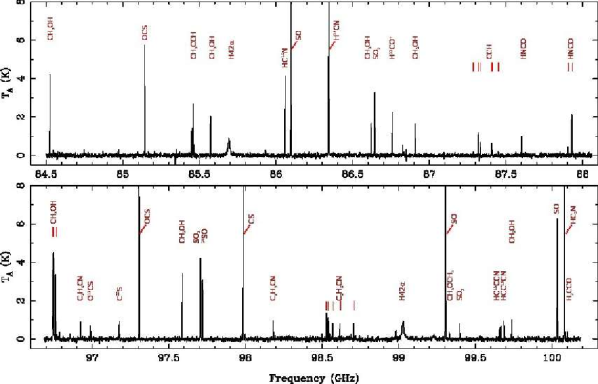
Figure 1: Continuum subtracted spectrum taken toward G345.49+1.47. Species associated with the most conspicuous lines are indicated.

To identify different molecular species we used CASSIS together with the Jet Propulsion Laboratory (JPL, Pickett et al., 1998) and Cologne Database for Molecular Spectroscopy (CDMS, Müller et al., 2005) spectroscopic databases. For each conspicuous spectral feature, we determine which species in the subset of detected ISM species given by CASSIS have $V_{\rm LSR}$ between $-6$ and $-17$ km s^-1. This $V_{\rm LSR}$ interval is within $5.5$ km s^-1 from the ambient $V_{\rm LSR}\approx-11.5$. We revise other lines with comparable or lower energy upper energy levels and comparable or higher Einstein spontaneous emission coefficients in order to discern which is the most likely molecule responsible of the examined lines. Once a candidate is assigned to a spectral feature, we compared the data with local thermodynamic equilibrium (LTE) models in order to confirm or reject the identification. Because the spectrum is not too populated, there is often only a single candidate molecule, and mostly two. Probable candidate species are also determined by previous detection toward other star formation regions (e.g., Blake et al., 1987; Gibb et al., 2000). To identify the line we follow the criteria defined in Herbst & van Dishoeck (2009, §3.3). For the COMs, we were able to identify at least three lines of the main isotopologue per species. An anti-coincidence — that is, a line that should be detected according to the predictions of the LTE model but is not observed — is taken as a strict rejection criterion.

In addition to the lines listed in Table 1, tentative detections of CH₃OCHO (methyl formate, sometimes also written as HCOOCH₃) and NH₂CHO (formamide) are presented. We do not include these in Table 1 because the low signal-to-noise ratio of these lines ($\lesssim 3$ at peak) impedes us from claiming detection of either species. In later sections we derive quantitative upper limits of these two and other undetected molecules.

3.2 Main Morphological Features of IRAS 16562$-$3959

In this section we analyze the morphology of the emission from different species detected toward IRAS 16562$-$3959 using the zero moment maps of the most prominent transitions of each species. To generate the zero moment maps we use the moment masking algorithm described in Dame (2011) and the CASA task immoments. FITS files of the zero moment maps are publicly available in Guzmán et al. (2018).

We note here that the most prominent feature of IRAS 16562$-$3959 — in continuum and in molecular line emission — is the central emission associated with the HC Hii region and HMYSO G345.49+1.47. Figures 2 and 3 show zero moment images toward the inner $23\arcsec\times 23\arcsec$ of IRAS 16562$-$3959, centered in G345.49+1.47, of representative transitions of all 22 molecular species detected (see Table 1). Figure 2 and 3 present the maps organized by visual inspection from those which show a clear strong source associated with G345.49+1.47 (like the sulfuretted molecule transitions) to those in which there is less obvious emission from the central HMYSO (e.g., SiO).

Figures 4 and 5 show zero moment maps centered in G345.49+1.47 but on a larger scale ($\sim 1\farcm 5\times 1\farcm 5$). These two figures show, respectively, the maps of two groups of species which display similar morphologies, as estimated from their 2D cross-correlations. The grouping and correlation calculations are described in more detail in Section 3.3. Figure 6 shows the zero moment map of the NH₂D $(1,1)$ transition, which is not part of neither of the two previous groups and displays a unique morphology. Finally, the CS, $J=2\shortrightarrow 1$ zero moment map (shown in Figure A.1) is not used in the analysis of this section because the emission is doubtless optically thick and heavily affected by short baseline filtering.

Besides CS, maps displaying strong negative features are those of H¹³CO⁺, H¹³CN (Figure 5), and SiO (Figure 4) and they should be interpreted with caution. In this work, we avoid extracting integrated fluxes from regions larger than $10\arcsec$. In any case, note that when measuring the flux arising from a compact source — like a molecular core — using the filtered map may be more adequate than using the map without short baseline filtering. This is because in the second case the intensities so measured include emission from material more homogeneously distributed within the clump, which we would not consider it to be part of the core.

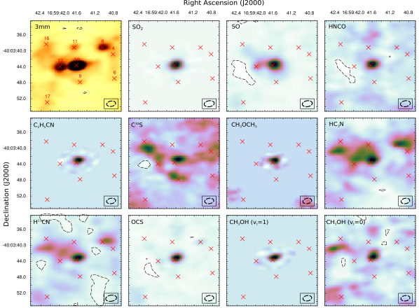
Figure 2: Zero moment maps of the emission from representative transitions from the central 23″$\times$23″region of IRAS 16562$-$3959. All these transitions show a strong, dominating source consistent with the position of G345.49+1.47 (Source 10). The upper left panel shows the continuum measured at 3 mm in a different color scale, together with the sources identified by Paper I. The name of several continuum sources are indicated in the first panel, and their positions are marked in the rest. The dashed contour level in the panels is $-0.03$ Jy beam^-1 km s^-1, corresponding to approximately $-5\sigma$. The dashed contours in the upper left panel correspond to those presented in Paper I.

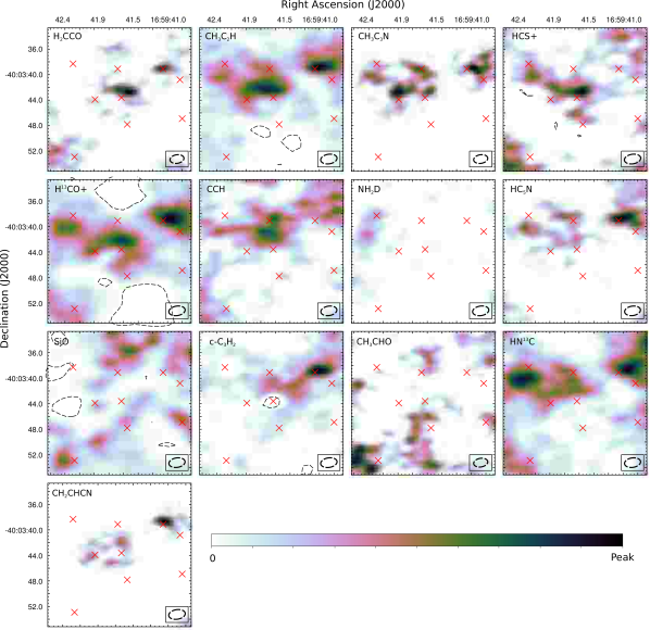
Figure 3: Same as Figure 2. Starting from the top left panel to the right and from top to bottom: the central source component becomes less and less prominent. Some transitions do not display a central dominating component at all, like the ones in the bottom rows.

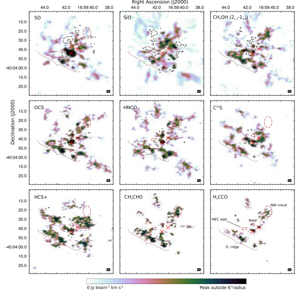
Figure 4: Zero moment maps of representative transitions of molecular species related with the Shock group (see Section 3.3). The dashed contour level in the panels is $-0.03$ Jy beam^-1 km s^-1, corresponding to approximately $-5\sigma$. The two red crosses mark the position of Sources 8 and 10. To ease comparison, we show the NW-cloud, the N-red cloud, the NEC-wall, and the position of the Diffuse Ridge together with the DR(a), (b), and (c) positions (black crosses) defined in Section 3.2 and Figure 7.

Figure 5: Same as Figure 4, but with species in the Continuum group (see Section 3.3). The top left panel shows the 3 mm continuum. Red crosses indicate the continuum sources 3, 7, 8, 10, and 16.

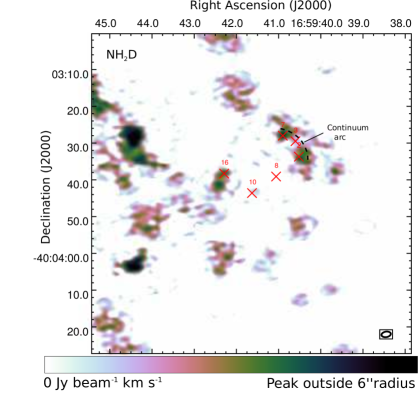
Figure 6: Zero moment map of the NH₂D $(1,1)$ transition. This species shows no evident similarities with either the Shock or Continuum group. We indicate the structure referred to as the “Continuum Arc” in Section 3.5.

Figure 7 shows maps of HC¹⁵N and CH₃OH and displays morphological features which are common to several molecular species. As explained in more detail in Section 3.3, these two molecules are representative of the two distinct groups we define to separate the species according to their morphology. The maps show emission from relatively low excitation lines, $E_{\textrm{up}}=21.6$ K for CH₃OH and $4.1$ K for HC¹⁵N. We also show position velocity diagrams (pv-diagrams) of the data cubes in the lateral and upper panels. The pv-diagrams display, for each position, the maximum intensity measured cutting through the other dimension of the cube. We find that this way of displaying was more effective in separating and identifying structures than the integrated intensity of the cubes collapsed in R.A. or declination.

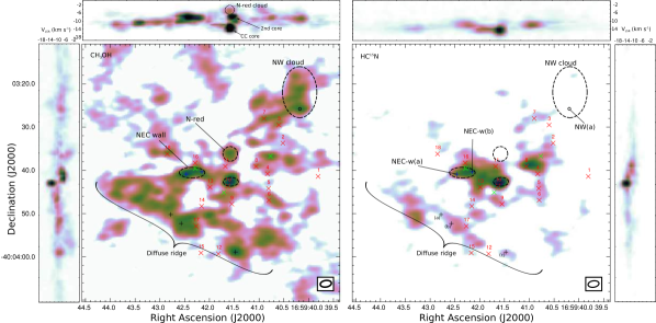
Figure 7: Panels a) and b) show zero moment maps of the CH₃OH, $({\rm E_{1}})$ $2_{1,1}\shortrightarrow 1_{1,0}$ ($E_{\textrm{up}}=21.6$ K) and the HC¹⁵N, $1\shortrightarrow 0$ ($E_{\textrm{up}}=4.1$ K) transitions, respectively. Red circles mark the continuum sources identified at 3 mm in Paper I. Green crosses show the position of the CH₃OH, $({\rm E_{2}})$ $5_{-1,0}\shortrightarrow 4_{0,0}$ maser spots. Black crosses mark the DR(a), (b), and (c) positions in the Diffuse Ridge, the NEC-wall (a) and (b) positions, and the NW-cloud (a) position (Section 4.2). Black-dashed ellipses mark the CC core, the N-red cloud, and the NW cloud. To the left and on top of panel a) we show R.A.-velocity and Declination-velocity pv-diagrams, respectively. In the top R.A.-velocity pv-diagram we mark the N-red cloud with a dashed circle, and two arrows indicate the sources which compose the blended CC core emission in the CH₃OH zero moment map. PV-diagrams of the HC¹⁵N emission are shown to the right and on top of panel b).

The main morphological features we identify are:

• A central compact core (CC core). The CC core is the most conspicuous feature in many of the transitions detected toward IRAS 16562$-$3959. The zero moment emission peaks near the central HC Hii region/HMYSO G345.49+1.47, marked as Source 10 ($\text{R.A.}=16^{\text{h}}59^{\text{m}}41\fs 63$, $\text{decl.}=-40\arcdeg 03\arcmin 43\farcs 6$) in Figure 2, but displaced from it — as noted in Paper I — between $0\farcs 4$ to $1\farcs 4$ in the northwest direction, depending on the specific tracer. continuum at 218 GHz and CH₃CN, $J=12\shortrightarrow 11$ (methyl cyanide) observations of IRAS 16562$-$3959 presented by Cesaroni et al. (2017) confirm that Source 10 actually consists of two peaks: one associated with the HMYSO/HC Hii region (G345.49+1.47) and another associated with a small ($\sim 0\farcs 5$), continuum source located $0\farcs 8$ northwest of G345.49+1.47. Figure 2 shows zero moment maps of molecules for which emission from the CC core is clearly distinguished. Some care is needed for the interpretation of the position based solely on these maps because, as shown in the pv-diagrams of Figure 7, the zero moment emission in the direction of the CC core is composed of two distinct cores with different radial velocities. We identify one of these cores as the CC core because it is centered at $V_{\rm LSR}=-15.4$ km s^-1, which is closer to the central velocity of the hydrogen recombination lines arising from the HC Hii region (Paper I) associated with G345.49+1.47. The CH₃OH pv-diagrams show that the second core (marked as ‘2nd core’ in Figure 7) is located $\approx 1.3\arcsec$ to the northwest (2″ from Source 10 in the $\textrm{P.A.}=-60\arcdeg$) and centered at $V_{\rm LSR}=-9.4$ km s^-1, that is, redshifted respect to G345.49+1.47. Figure 7 shows these two cores in the R.A.-velocity diagram of CH₃OH. Some emission from the secondary redshifted core is detected in HC¹⁵N, but much fainter than the proper CC core centered at $\approx-15.4$ km s^-1. This secondary redshifted core is likewise evident in emission from other species such as H¹³CO⁺, HC₃N, and HN¹³C.

• Source 8 core (C8). Many molecules show strong and extended emission near the source marked with number 8 in Figure 2. We note, however, that the molecular peak is not coincident with the continuum peak. Usually, the molecular emission is strongest between $0\farcs 5$ and $1\farcs 5$ in the $\textrm{P.A.}=-15\arcdeg$ direction from Source 8. This is the case of COMs like HC₅N, CH₃C₃N, CH₃CCH, and CH₂CHCN, where the emission usually spreads toward the NE direction forming an elongated cloud. A methanol maser seems to be associated with the outer rim of this molecular envelope.

• A Diffuse Ridge. It is shown in Figure 7 as the elongated methanol emission feature crossing the south east part of IRAS 16562$-$3959. This structure appears most prominently in CH₃OH, CH₃CHO, and in most other tracers shown in Figure 4. The Diffuse Ridge extends for $\approx 40\arcsec$ in the $\textrm{P.A.}=65\arcdeg$ direction from the position $\Delta\textrm{R.A.}=-10\arcsec,\quad\Delta\textrm{Dec.}=-15\arcsec$ respect to G345.49+1.47. Within the Diffuse Ridge there are two distinct emission cores. One is marked with a ’(b)’ in Figure 7 and is centered at $\Delta\text{R.A.}=+10\arcsec,\Delta\text{dec.}=-9\arcsec$ from Source 10, with a diameter of $\approx 5\arcsec$. The other, marked with a ’(c)’, is located at $\Delta\text{R.A.}=-2\arcsec,\Delta\text{dec.}=-15\farcs 5$ from Source 10, slightly elongated in the direction $\text{P.A.}=75\arcdeg$ with diameters of $\approx 5\arcsec\times 3\arcsec$. Position ’(a)’, on the other hand, targets more diffuse gas forming the body of this ridge or filament. Hereafter, we refer to these three positions as DR(a), DR(b), and DR(c). DR(b) is conspicuous in CH₃OH and likewise in CH₃CHO, SiO, SO, HCS⁺, OCS, CS, HC₃N, and HNCO. It is less noticeable in HN¹³C, H¹³CN, and C³³S, but still present. DR(c) is as well distinguished in CH₃CHO, SiO, SO, OCS, CS, HNCO, and H¹³CN. Emission from DR(c) is also detected in H¹³CO⁺ and HC₃N. In contrast with DR(b), we do not detect HN¹³C nor HCS⁺ emission associated with DR(c).

• A northeast outflow cavity wall (NEC-wall). This molecular feature located $\approx 2\arcsec$ south of Source 16 matches an illuminated section of the outflow cavity wall seen in NIR. The emission is conspicuous in CH₃OH, CH₃C₃N, CCH, HC₃N, HC₅N, H¹³CN, HN¹³C and H¹³CO⁺ transitions. Other molecules display emission farther from the cavity wall position, but still associated with it, like c-C₃H₂, C³³S, CH₃CHO, OCS, and maybe SO. The large scale emission from SiO and HNCO which surrounds the NEC-wall area is not clearly associated with it.

• A northwest cloud (NW cloud). This emission cloud has approximately $5\arcsec\times 3\arcsec$ of size and it is centered around the position located approximately 25″ in the $\textrm{P.A.}=-50\arcdeg$ direction respect to the CC core. This feature is displayed by most of the molecules shown in Figure 4, including CH₃OH, SiO, CH₃CHO, HNCO, and CS. There is also strong emission associated with HC₃N. Less prominent emission arises from H¹³CN, HN¹³C, H¹³CO⁺, CCH, H₂CCO, HC₅N, OCS, and SO as well.

• A northern redshifted cloud (N-red cloud). This emission feature of $\approx 1.5\arcsec$ radius is specially conspicuous in transitions shown in Figure 4. It is one of the emission cores with the largest differences in radial velocity respect to the clump. In methanol, its radial velocity is centered at $-7.5$ km s^-1, that is, redshifted by $4.1$ km s^-1 respect to the $V_{\textrm{LSR}}$ of IRAS 16562$-$3959. Molecules which display strong emission toward the N-red cloud are (besides CH₃OH) SiO, HNCO, OCS, CS, and SO. Less prominent emission is detected from HC₃N, CH₃CHO, and H₂CCO. In each case, the emission is consistently redshifted respect to the systemic radial velocity of the clump. The N-red cloud is located $\sim 7\arcsec$ north of the CC core and is not to be confused with the ‘2nd redshifted core’ we mentioned previously.

3.3 Zero Moment Cross Correlations and Grouping

In order to evaluate quantitatively how similar are the zero moment maps of different species, we calculate the cross correlation between each pair of maps according to

$$\rho_{12}=\frac{\sum_{i,j}I_{1,ij}I_{2,ij}w_{ij}}{\left(\sum_{i,j}I^{2}_{1,ij}w_{ij}\sum_{i,j}I^{2}_{2,ij}w_{ij}\right)^{1/2}}~{}~{},$$ (1)

where the sums are taken over each pixel position, $I_{1,ij}$ and $I_{2,ij}$ are the values measured for each image at pixel $i,j$, and $w_{ij}=0,1$ defines the masked region used for the calculation. Note that by definition $\rho_{12}=\rho_{21}$ and $|\rho_{12}|\leq 1$. A value of $\rho_{12}=1$ implies that $I_{1}=\alpha I_{2}$, with $\alpha$ a positive constant. Therefore, the more similar the zero moment spatial distributions are, the closer their cross correlation is to 1.

According to the definition of Equation (1), brighter sections of the image weight more into the calculation of $\rho_{12}$. In order to avoid the correlation being dominated entirely by the central source, we mask the pixels (that is, we set $w_{ij}=0$) inside an inner circle of 6″ radius centered at G345.49+1.47. We leave outside this specific analysis some molecules which are only detected toward the center of the field, e.g., CH₃CH₂CN, ¹³CH₃OH, and SO₂.

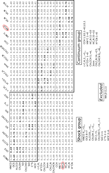
Figure 8: Cross correlations between zero moment maps of molecules with significant extended emission, and with the continuum (marked with 3 mm). For each molecule, the maximum correlation is marked in boldface. Each molecule in any of the two enclosed frames has their maximum correlation partner in the same group they pertain. The top left and bottom right framed groups correspond to the so called Shock and Continuum groups, respectively. Below the cross correlation matrices we list explicitly the members and the specific transition used. For completeness we include NH₂D despite this molecule not being part of either group.

Figure 8 displays the value of the cross-correlations between the zero moment maps of different molecules. We include in this analysis the continuum image at 3 mm presented in Paper I. In order to gather together molecular emission based on their spatial distributions, we will use the $\rho_{12}$ value as a measure of morphological similarity. Cross correlations have been used to this end (although comparing only with the continuum) by Lu et al. (2017). For each molecule, we determine which one is the other species (among the set of molecules in this study) with the highest cross correlation. We call this species the maximum correlation partner (MCP) of the considered molecule. We stress that this relation is not necessarily symmetric: for example, while OCS and CH₃OH are MCPs of each other, OCS is the MCP of SO but not vice-versa. The cross correlation values of MCPs are marked in boldface in Figure 8.

Figure 8 shows that molecules gather in two groups by linking them together with their MCPs. That is, the MCP of each molecule in any of these groups is within that same group. In this way, we gather together molecules with similar zero moment morphologies. Visual inspection of the maps confirm this interpretation, except in the case of NH₂D, which has the lowest cross correlations with its MCP (0.39). Because the zero moment map of this molecule (Figure 6) is so different compared to the rest, we do not include it in the grouping and we analyze it independently. We estimate the uncertainty of $\rho_{12}$ by adding simulated noise to each zero moment map and measure the dispersion of the values of the cross correlations thus obtained. In all cases, the uncertainty due to random noise is $<0.01$, making no discernible effect in the classification.

We denominate “Shock group” the one in which traditionally shock activity tracers such as SiO, HNCO and SO gather. We refer to the second group as the “Continuum group” because it gathers species better correlated with the 3 mm continuum. As Figure 8 shows, the MCP of the continuum image is the zero moment of the H¹³CO⁺, $J=1\shortrightarrow 0$ transition.

We warn that the specific numerical value of the correlation is probably affected by instrumental and observational effects such as the uv-coverage, the pointing within IRAS 16562$-$3959, and the primary beam shape (though not by constant calibration factors). This means that how these cross correlations compare between each other is more important than the specific values presented in the matrix shown in Figure 8. One possible caveat of this way of calculating similarities between the molecules is the non inclusion of kinematic data, that is, it is possible that the zero moment of two molecular transitions are very similar, but their lines having very different central velocities. Thus, we calculate the cross correlations using the data cubes of the lines in order to test whether the grouping described depends on ignoring the kinematic information. We find that the same grouping as described in Figure 8 occurs, so we keep the simpler approach of calculating cross correlations using the zero moment images, which also allows us to calculate correlations between images of the molecular lines and the continuum.

3.4 Kinematics

We analyze the kinematics of IRAS 16562$-$3959 using first moment maps. Figure 9 shows first moment maps of those molecules with resolved kinematic features and strong extended emission. We leave out molecules with only emission toward the CC core like CH₃OCH₃, CH₃CH₂CN, and SO₂: first moment maps of the first two are rather uninformative because they display no velocity gradients and seem to be well characterized by a single $V_{\rm LSR}$. The SO₂ map, on the other hand, does show a velocity gradient characteristic of rotation which was analyzed in detail in Paper I. We also leave out species with only faint extended emission like HC₅N, CH₃C₃N, CH₂CHCN and H₂CCO. The first moment maps of these molecules display similar characteristics as those shown in Figure 9, but with lower signal-to-noise ratios.

We stress that the kinematic analysis is somewhat hindered by the modest spectral resolution of the data. Figure 9 shows that the velocities range between $-8$ and $-15$ km s^-1 for most molecules, with the ambient cloud velocity around $-12$ km s^-1. This is consistent with previous single dish studies on IRAS 16562$-$3959 (Bronfman et al., 1996; Urquhart et al., 2007; Miettinen et al., 2006).

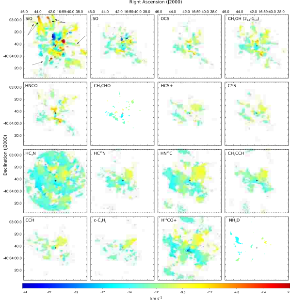
Figure 9: Large scale images of the first moment from molecular transitions with extended emission. To calculate the first moment, we masked emission below 5 mJy beam^-1 ($\sim 5\sigma$). Black crosses indicate the position of G345.49+1.47. Black arrows in the SiO panel indicate some of the so-called “fingers.”

On a large scale, most molecules display redshifted velocities ($\sim-10$ km s^-1, that is, redshifted respect to the ambient cloud) toward the north west section of IRAS 16562$-$3959, and blueshifted velocities ($\sim-14$ km s^-1) toward the south east. This trend is reminiscent of the general orientation of the jet and CO outflow detected toward G345.49+1.47 (Guzmán et al., 2011). This general kinematic trend is well illustrated by the H¹³CO⁺ first moment map, but it is also evident in HC₃N, HC¹⁵N, HN¹³C, CH₃CCH, c-C₃H₂, and C³³S. The trend is less evident — but still tantalizing — in SO, CH₃OH, HC₅N, CCH, and even NH₂D . The H¹³CO⁺ map likewise displays conspicuous blueshifted emission located about $4\arcsec$ south of G345.49+1.47, which is due to gas with $V_{\rm LSR}\approx-19.1$ km s^-1. This emission is apparent in HC¹⁸O⁺ and SO, but it is not clearly seen in any other molecule.

By far, the transition showing the largest velocity variations across the field is SiO, $J=2\shortrightarrow 1$. These variations, illustrated in the first panels of Figure 9, span $20.9$ km s^-1, whereas for the rest of the molecules the velocity span is $\lesssim 10$ km s^-1. Interestingly enough, the only exception to this trend is SO, whose velocity span is $\sim 14.8$ km s^-1. This kinematic feature of SO is consistent with the similar morphology observed between its zero moment map and that of SiO.

Another kinematic feature unique to SiO are the conspicuous filaments or “fingers” populating the north east region of IRAS 16562$-$3959, which extend roughly in the radial direction from G345.49+1.47. As shown in Figure 9, these features are associated with velocity gradients of the order of $\sim 10$ km s^-1 across a distance of 30″ (0.25 pc at 1.7 kpc). Four discernible “fingers” are located toward the north east region of the clump. Additional fingers are apparent toward the south east and western parts of IRAS 16562$-$3959. These fingers of SiO emission are presumably outflows or outflow cavities generated by other YSOs in IRAS 16562$-$3959. However, the structures are as well reminiscent of the “explosive” streamers found toward OMC1 (Bally et al., 2017) and DR21 (Zapata et al., 2013), in the sense that many of them seem to point toward the center of the clump. Further investigation will determine what is the true nature of these structures only apparent in SiO emission.

Finally, we note that besides SO, SO₂ — and isotopologues — there is no other molecule associated with the velocity gradient characteristic of the rotating core around G345.49+1.47 detected in Paper I.

3.5 Morphology of the Emission by Molecule

In the following paragraphs we describe the main characteristics of the emission of representative transitions of each species. This section expands the description of Section 3.2 focusing on the specific morphology per molecule. Paper I already analyzed in detail the morphology of most of the sulfuretted molecules emission near the central HMYSO, so we refer to their analysis for these species (SO, SO₂, OCS, CS and their isotopologues). To organize the upcoming discussion we gather the molecules according to their composition and number of atoms.

3.5.1 Simple molecules

With simple molecules we refer to molecules with 5 atoms or less.

Nitrogenated. We include here the HCN isomers, HC₃N (cyanoacetylene) and , and NH₂D. Just for the sake of exposition, we choose to include HNCO. The regions where HC₃N (and the ¹³C isotopologues) emission is most intense are the CC core, the NEC-wall, and C8. The C8 emission peaks $\sim 0\farcs 7$ to the west from Source 8. An extended, distinct HC₃N emitting region is a triangular-like structure between sources 10, 11, and an emission peak located $1\farcs 3$ north of source 13 (see Figure 2). Emission from the ¹³C isotopologues displays the same morphological features. On a clump scale, emission from HC₃N is most similar, as evaluated from the cross correlations, to HN¹³C and H¹³CN. Figure 5 suggests in addition good match between the HC₃N zero moment map and those of H¹³CO⁺ and CH₃CCH, which is confirmed by the cross-correlations.

Other nitrogenated simple molecules are the isotopologues H¹³CN and HC¹⁵N. Their zero moment maps are very similar, with a cross correlation of 0.9, which is higher than any correlation between different species ($\leq 0.8$). The correlation calculated masking the central dominant source (Section 3.3) is $0.86$. Kinematically, the molecules are similar as well. The linewidths range between the 2 and 6 km s^-1, with most of the emission having linewidths between 3 and 4 km s^-1.

An evident difference between the line profiles of H¹³CN and HC¹⁵N is the hyperfine splitting of the $J=1\shortrightarrow 0$ H¹³CN  transition produced by the nuclear quadrupole of the ¹⁴N nucleus. We fit Gaussians to the three hyperfine components in order to explore further the observed splitting. The blue and redshifted components are located at velocities of $-7.3$ and $+4.9$ km s^-1 respect to the central component, which is the brightest. Theoretically, the line intensities should be in the $1:5:3$ ratio in optically thin conditions. We performed the fitting in every pixel where the peak intensity exceeds 5 $\sigma$. The observed intensity ratios of the blue and redshifted components respect to the central one are $1\pm 0.5:5:2\pm 1$ respectively, where the uncertainties represent the standard deviation of these quotients measured throughout the field. The blueshifted versus the central component ratio appears to concur with theory, while the redshifted component ratio is slightly lower than expected, but consistent with the observed 1-$\sigma$ variations. We conclude that our results are consistent — within the uncertainties — with the local thermodynamic equilibrium and optically thin predictions.

The morphology of the HN¹³C emission resembles that of H¹³CN: they both display strong emission associated with the C8 and the NEC-wall. However, there are two important differences, the most relevant being the complete absence of HN¹³C emission from the CC core while H¹³CN is bright there. The other noticeable difference is the HN¹³C emission associated with the arcuate continuum structure joining sources 7, 3, 2, and 8. Because this arc of emission appears conspicuously in a few other transitions, we refer to it hereafter as the Continuum Arc.

HNCO (isocyanic acid), on the other hand, is a molecule with a strong CC core component. Its zero moment maps are well correlated with those of OCS and CH₃OH, showing strong emission associated with the Diffuse Ridge, the NW cloud, and the N-red cloud. However, there is not much HNCO emission associated with the C8 or the Source 8 itself, and no emission associated with the NEC-wall. Isocyanic acid is the only nitrogenated species in the Shock group.

Finally, NH₂D is a special case. By and large, the zero moment of NH₂D (Figure 6) displays little correlation with features conspicuous in other molecules, and we analyze it separately from the Shock or Continuum groups. The peak of the NH₂D emission is located $36\arcsec$ from G345.49+1.47, in the $\text{P.A.}=65\arcdeg$ direction. This NH₂D core is apparently part of a filament which extends for $\approx 30\arcsec$. Molecules which have emission related with the location of this core are HN¹³C, CCH, and possibly HCS⁺. A secondary peak of NH₂D emission is associated with a core located $38\arcsec$ south east of G345.49+1.47, in the $\text{P.A.}=122\arcdeg$ direction. This core is not related with any discernible structure in any other molecule, but, as seen below, it seems related with a NIR-dark globule. Less intense emission is located associated with the NEC-wall and with Source 16, and there is also emission connecting both positions. This morphology resembles the continuum (Paper I), which shows that Source 16 is embedded in an envelope extending to the south until approximately the region we identify in this work with the NEC-wall. Other features clearly associated with NH₂D emission are Sources 7 and 2 and some diffuse emission apparently tracing the Continuum Arc. As we will see below, it does show some faint emission associated with the CC core, barely noticeable in Figure 3.

Sulfuretted. A rather complete analysis of the morphology of the emission from the sulfuretted molecules, specially in the central region of IRAS 16562$-$3959, is given in Paper I. They concluded that sulfur oxides (SO, SO₂, and isotopologues) are well associated with G345.49+1.47, in contrast to other carbon-sulfur species such as OCS and CS. All sulfuretted species whose emission extends on scales comparable with the clump size — that is, all of them except SO₂ — are in the Shock group. From Figures 4 and 8 it appears that SO and OCS correlate more with CH₃OH and (ignoring the CC core) SiO than with other sulfuretted molecules like C³³S and HCS⁺. The zero moment maps of these last two molecules are similar between each other, and they display some features observable in some molecules of the Continuum group (like CCH, see below).

The only sulfur bearing molecule which was not included in Paper I is HCS⁺. Figures 3 and 4 show the zero moment of the HCS⁺, $J=2\shortrightarrow 1$ line. Figure 3 shows that there is emission apparently related with the CC core, but more extended and located $\sim 0\farcs 4$ farther to the north from G345.49+1.47 compared to than that of, e.g., methanol. On a larger scale, Figure 4 shows that the HCS⁺ emission is most similar to that of C³³S. This similarity is reflected in the velocity distribution of both lines.

Two of the most remarkably similar zero moment maps are those of SO and SiO (see Section 3.3), whose similarity is also observed in the first moment maps (see Section 3.4). Several common features are recognizable in these two maps (Figure 4), but one equally remarkable difference is the strong emission from SO associated with the CC core, which is absent in SiO. That is, the SO emission in IRAS 16562$-$3959 can be characterized by a strong, rotating CC core (described in Paper I, ) surrounding G345.49+1.47, plus spatially extended emission well correlated with SiO. This behavior of SO is somewhat reflected in the rest of the sulfur bearing molecules, all of them part of the Shock group.

Finally, we note that the CS zero moment map (Figure A.1) is less similar than expected to that of C³³S. We attribute this to the high optical depth of CS compared to that of the C³³S.

Small carbon chains. In this category we include CCH and c-C₃H₂, the latter being a cyclic molecule. Neither of these two molecules have emission associated with the CC core, with c-C₃H₂ displaying an strong absorption feature toward the location of G345.49+1.47, centered at $-13.6\pm 0.1$ km s^-1 with a FWHM of $4.6\pm 0.3$ km s^-1. One important feature of the CCH, $N=1\shortrightarrow 0$ transition line is that it splits in six hyperfine components (discernible in Figure 1). The relative observed strength of these components (whose temperature dependence is negligible) is in good agreement with the ratio expected for optically thin emission. CCH emission is strongest in the Continuum Arc, specifically, just below Source 3. Its is likewise strong between the CC core and N-red cloud, in the NEC-wall, and in a cloud located $\sim 20\arcsec$ to the south east of G345.49+1.47 ($\textrm{P.A.}=135\arcdeg$). This last emission feature is also conspicuous in the zero moment map of c-C₃H₂ and it has no obvious counterpart in any other molecule.

Emission from c-C₃H₂ seems to be less extended compared to that of CCH. It is strongest in the C8 region, extending somewhat toward the Continuum Arc. As pointed out before, there is clear emission associated with the south east cloud mentioned above. Contrary to CCH, there is no strong c-C₃H₂ emission arising from the NEC-wall. Less prominent c-C₃H₂ emission is also detected from a cloud located at $\sim 22\arcsec$ to the east of G345.49+1.47 ($\textrm{P.A.}=80\arcdeg$). We note that there is evident CCH and C³³S emission from this region as well.

Additional similarities between CCH and C³³S include a filament of emission extending for $\sim 15\arcsec$ roughly in the E-W direction, located $30\arcsec$ north east of G345.49+1.47 ($\textrm{P.A.}=45\arcdeg$). We note that this filament is also visible in HCS⁺.

Oxygenated. In this category we analyze simple molecules composed of carbon and oxygen, that is, the isotopologues H¹³CO⁺ and HC¹⁸O⁺ and H₂CCO (ethenone). The HC¹⁸O⁺ map is very similar to that of H¹³CO⁺ (correlation coefficient of 0.79), with the HC¹⁸O⁺ line being more optically thin ($\approx 8$ times less abundant according to Wilson & Rood, 1994) compared with H¹³CO⁺. Figure 3 shows that the emission from H₂CCO and H¹³CO⁺  is associated with the CC core and C8. The H₂CCO zero moment map displays a more compact distribution around these two locations compared to that of H¹³CO⁺ or HC¹⁸O⁺.

On a large scale, both species are different: H₂CCO and H¹³CO⁺ were classified in the Shock and Continuum groups, respectively. Ethenone displays a good resemblance to the OCS (its MCP) and CH₃CHO maps, and the cross correlations given in Section 3.3 are practically equal (0.60 and 0.59, respectively). We can identify clearly in the H₂CCO map, emission coincident with the Diffuse Ridge, the NW cloud, and the N-red cloud. In addition, the H₂CCO map shows diffuse emission located $30\arcsec$ north of G345.49+1.47, which is seen clearly in OCS, CH₃CHO, HNCO, and CH₃OH.

The H¹³CO⁺, on the other hand, is the MCP of the 3 mm continuum map. That is, the H¹³CO⁺  zero moment map (Figure 5) is the one which better correlates with the continuum away of the central source, dominated by thermal dust . H¹³CO⁺ is one of the few molecules with counterpart emission associated with Source 13 (Figure 3). The zero moment map also shows a source located $\sim 4\arcsec$ south of G345.49+1.47 whose emission is significantly blueshifted respect to the ambient material (see Section 3.4). Other regions associated with strong H¹³CO⁺ emission are the NEC-wall and the C8. The C8 emission extends to the Continuum Arc. In addition, there is a south east diffuse feature which correlates roughly with the position of continuum Sources 12, 15, and 17.

Finally, we note that the H¹³CO⁺ emission, as it is the case for HC₃N and CH₃CCH, is more compactly distributed. There is little H¹³CO⁺ emission more than $20\arcsec$ away from G345.49+1.47, which is in stark contrast compared to the molecules of the Shock group.

3.5.2 Complex Organic Molecules (COMs)

COMs detected in this work are molecules consisting of carbon and hydrogen atoms plus, except CH₃CCH, either one oxygen or one nitrogen atom. The only molecule detected with an O and a N atom is HNCO, and we do not detect any molecule with more than one N or O atom. In the following, we call a molecule saturated if all its carbon-carbon bonds are single (C−C). Conversely, unsaturated COMs have double or triple carbon-carbon bonds (C=C or C≡C). All simple molecules with carbon-carbon bonds detected in this work (CCH, c-C₃H₂, HC₃N, and H₂CCO) are unsaturated, but this is likely due in part to a selection effect: saturated hydrocarbons usually have more atoms.

Propyne (CH₃CCH). This COM was previously observed toward IRAS 16562$-$3959 using single dish by Miettinen et al. (2006). The central region (Figure 3) shows some correlation with the CC core, but with the bulk of the emission arising north of G345.49+1.47. The propyne zero moment peak is located $2\arcsec$ north-east of G345.49+1.47. Propyne is also brightly associated with the C8: a secondary emission peak is located less than $1\arcsec$ west of Source 8. On a larger scale (Figure 5), CH₃CCH emission displays a rather smooth distribution, with a very good correlation with H¹³CO⁺, although less bright. These two molecules are MCPs of each other. Practically all the bright features distinguished in the H¹³CO⁺ zero moment map have a CH₃CCH counterpart. Propyne shows a good correlation with HC₃N as well, excluding the central region. Due to the difficulty in separating the different CH₃CCH lines due to blending, the zero moment maps shown include the sum of all the $5,K\shortrightarrow 4,K$ transitions.

Nitrogenated (CH₃CH₂CN, CH₃C₃N, CH₂CHCN, and HC₅N). Only one of these COMs, propanenitrile (CH₃CH₂CN, hereafter C₂H₅CN), is unequivocally linked with the CC core. Figure 2 shows that the emission from this COM peaks close to G345.49+1.47, but displaced from it by $\sim 0\farcs 5$ compared to SO₂ or HNCO. Faint emission of C₂H₅CN (not evident in the zero moment map image) is detected also toward the C8 (see Section 6). We do not detect this COM toward any other location in the clump.

As shown in Figure 3, the other three COMs have less correlation with the CC core, and none of their peaks actually correspond with the CC core position. Among these COMs, CH₃C₃N (cyanopropyne) is the only one which shows some CC core counterpart. The emission from CH₃C₃N has two peaks, associated with the NEC-wall and C8, with practically the same intensity. The C8 CH₃C₃N emission peaks approximately $1\arcsec$ east of Source 8, and extends somewhat to the Continuum Arc. The NEC-wall emission from this COM apparently joins with the CC core emission and with emission detected south of Source 16. The overall appearance of this structure is similar to what is observed in other molecules, for example, HCS⁺ (same Figure 3). There is emission correlated with the position of Source 11, which is a feature seen in a few other molecules (e.g., CCH, CH₃CCH, and HN¹³C). Figure 5 shows the CH₃C₃N zero moment map on a larger scale. There is not much more emission compared with what is shown in Figure 3. However, we note a small cloud located about $18\arcsec$ south west from G345.49+1.47 in the $\text{P.A.}=-135\arcdeg$ direction. Emission from this location is clearly detectable in CCH, CH₃CCH, H¹³CN, HN¹³C, H¹³CO⁺, HC¹⁵N, HC₃N, HCS⁺, and CH₂CHCN. It is located near the south west end of the Diffuse Ridge, thus, we can better discern it in molecules without Diffuse Ridge emission like CCH and CH₃CCH.

Emission from acrylonitrile (CH₂CHCN, hereafter C₂H₃CN) is better displayed in Figure 3, because most of the emission arises from regions not farther than $15\arcsec$ from G345.49+1.47. The peak of C₂H₃CN emission is clearly associated with C8. Acrylonitrile is one of the faintest molecule we claim detection in this work. With the exception of the peak emission, the rest of the features shown in Figure 5 are apparently real mostly because their location is consistent with emission seen in other molecules. There is also emission somewhat consistent with the CC core and with the south west cloud described at the end of the previous paragraph.

Finally, Figures 3 and 5 show the zero moment images of the cyanopolyyne HC₅N (cyanodiacetylene). This molecule does not show strong emission associated with the CC core. Weak emission located $\approx 1\arcsec$ north of G345.49+1.47 joins to the east with emission arising from the NEC-wall, as seen in many other molecules. As it is likewise the case for CH₃CCH, CH₃C₃N, CCH, and HN¹³C, there is HC₅N emission associated with the location of Source 11. The HC₅N peak is clearly located in C8. Diffuse emission extends from the C8 to the north following somewhat the Continuum Arc. Relatively intense, diffuse emission, is also associated with Source 7.

Oxygenated (CH₃OH, CH₃CHO, and CH₃OCH₃). By far, the CH₃OH (methanol) transitions display the brightest and richest spatial structures of all COMs. Among the eleven detected methanol lines there is one rotational line from a vibrationally excited state and a class I maser transition (${\rm(E_{2})}$ $J_{K_{a}K_{c}}=5_{-1,0}\shortrightarrow 4_{0,0}$). Methanol emission (Figures 2 and 4) is in every line dominated by strong emission detected toward the CC core, except for the maser transition which is dominated by three bright maser “spots.”

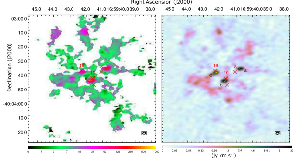
Figure 10: Left panel: Ratio between the zero moment of the CH₃OH, ${\rm(E_{2})}$ $J_{K_{a}K_{c}}=5_{-1,0}\shortrightarrow 4_{0,0}$  and $2_{1,1}\shortrightarrow 1_{1,0}$ lines. Right panel: Zero zero moment of the CH₃OH, ${\rm(E_{2})}$ $J_{K_{a}K_{c}}=5_{-1,0}\shortrightarrow 4_{0,0}$ emission. The three masers (yellow circles) correspond to the three strongest sources (whose coordinates are given in Table 3), conspicuous even in the logarithmic color stretch. Red crosses and numbers show continuum 3 mm sources nearby the masers.

Figure 10 shows in the left panel the quotient between the zero moment maps of the ${\rm(E_{2})}$ $J_{K_{a}K_{c}}=5_{-1,0}\shortrightarrow 4_{0,0}$ and $2_{1,1}\shortrightarrow 1_{1,0}$ CH₃OH transitions. The three maser spots marked a, b, and c in the right panel of this figure (which shows the zero moment of the maser transition in logarithmic color stretch) are associated with line fluxes more than 100 times larger than those of the typically thermal $2_{1,1}\shortrightarrow 1_{1,0}$ line. Table 3 indicates the parameters of the maser emission. The strongest maser is b followed closely by a. Maser a is located $4\arcsec$ in the $\text{P.A.}=-53\arcdeg$ direction from Source 8 and it is associated with bright methanol emission in the rest of the lines. Other molecules which show clearly emission consistent with the location of Maser a are CH₃CHO and H₂CCO, and perhaps less clearly HCS⁺ and OCS. Methanol lines associated with low upper energy levels ($<50$ K) are characterized by brighter emission toward the Maser a location than toward Source 8, whereas the opposite is true for high energy transitions ($>50$ K). Source 8 is also bright in H₂CCO and OCS but not in CH₃CHO. Maser b is located $1\farcs 6$ to the south east($\text{P.A.}=150\arcdeg$) from G345.49+1.47. Due to the proximity of the CC core, this region is associated with diffuse emission in several molecules. However, in contrast with Maser a, there is no distinguishable feature in either methanol or any other molecule coincident with the position of this maser. Maser c, located $1\farcs 4$ south of Source 16, seems to be associated with the NEC-wall.

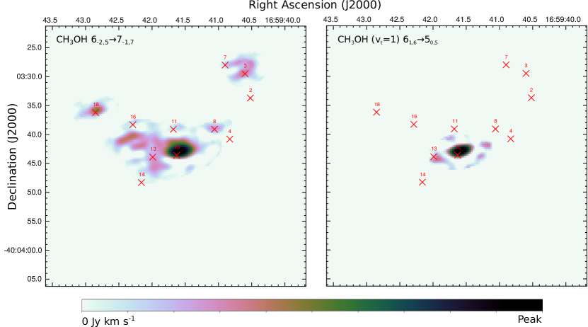
Figure 11: Left and right panels show, respectively, the zero moment maps of the CH₃OH, $6_{-2,5}\shortrightarrow 7_{-1,7}$ and $6_{1,6}\shortrightarrow 5_{0,5}$ ($v_{t}=1$) transitions. Red crosses and numbers show the position of continuum 3 mm sources as defined inPaper I. The upper energy levels of these two transitions are $74.7$ and $340.1$ K, respectively.

Partly because of the intricate details observed in methanol we used the zero moment map of CH₃OH, $2_{1,1}\shortrightarrow 1_{1,0}$ to define some of the most noticeable of IRAS 16562$-$3959 (Section 3.2). In that analysis we used a comparatively low energy transition ($E_{\textrm{up}}=21.6$ K). Higher energy transition zero moment maps are expected to be less rich, but they emphasize different features. Figure 11 shows the zero moment maps of two higher energy transitions, one with $E_{\textrm{up}}=74.7$ K and the other $340.1$ K. The latter shows only the CC core, and perhaps some emission associated with Source 13. The CC core emission in this highly excited state of CH₃OH supports the view that this is a HMC. The $6_{-2,5}\shortrightarrow 7_{-1,7}$ ($E_{\textrm{up}}=74.7$ K ) transition does show more structure: besides the CC core, which is the dominating source, there is diffuse emission connecting the northern part of the CC core with the NEC-wall. There is in addition diffuse emission extending south $\approx 5\arcsec$ at the R.A. of Source 13. We note that while the low energy methanol (Figure 7) shows extended diffuse envelopes blending in with the continuum sources, the left panel in Figure 11 shows a much less ambiguous correlation with Sources 7, 3, 8 and 18. Structures which are not apparent in the high energy CH₃OH transitions are the Diffuse Ridge, the NW cloud, and the N-red cloud.

Acetaldehyde (CH₃CHO) is another oxygenated COM we detect toward IRAS 16562$-$3959. Zero moment maps of this molecule are shown in Figures 3 and 4. The central region (Figure 3) immediately shows that CH₃CHO is not associated with the CC core. In fact, there is no clear emission associated unambiguously with any continuum source. On a larger scale (Figure 4) CH₃CHO emission shows features characteristic of the Shock group: its MCP is CH₃OH, with a correlation coefficient between them of $0.72$ (we emphasize that Section 3.3 uses a low energy CH₃OH transition for the analysis). Acetaldehyde is bright toward the Diffuse Ridge, the N-red cloud, the NW cloud, and Maser a position. In general, there is CH₃CHO emission toward bright methanol regions, e.g.: the diffuse CH₃CHO emission south of the CC core has a similar morphology as CH₃OH; a small cloud located $1\farcs 5$ west of Source 6 is bright in many Shock molecules, including CH₃CHO; and the cloud located $30\arcsec$ north of G345.49+1.47 already mentioned in the H₂CCO description.

Finally, CH₃OCH₃ (methoxymethane) is detected only toward two locations: the CC core and Source 8. The CC core CH₃OCH₃ emission is evident in Figure 2, but that of Source 8 is very faint and more evident in the data cube of the $4_{1,4}\shortrightarrow 3_{0,2}$ transition.

4 COLUMN DENSITIES AND EXCITATION TEMPERATURES

In this section we model the data and results presented in the previous sections and determine physical parameters like column densities and temperatures, mainly from LTE models. Section 4.1 focuses on the CH₃CCH emission and LTE modeling. Section 4.2 makes more detailed models of the emission of the species detected toward several sources in IRAS 16562$-$3959.

While the focus of the present work is on the detected species, as a general remark for the upcoming discussion we mention some noticeable non-detection and molecules whose lines were not covered by our observations. In addition to CH₃OCHO and NH₂CHO (mentioned in Section 3.1), other molecules commonly associated with hot-cores (e.g., Gibb et al., 2000) which were observed but not detected are HCOOH (formic acid) and CH₃CH₂OH (ethanol). These non-detection allow us to estimate upper limits on the column densities of the respective species (Section 4.2). On the other hand, neither H₂S (hydrogen sulfide), CH₃CN (methyl cyanide), nor their isotopologues were covered by our observations. The spectral setup does not efficiently cover the H₂CO (formaldehyde) or the HDCO lines either because it only samples transitions predicted to be faint (high $E_{\rm up}$ or very low Einstein $A$-coefficients).

4.1 Propyne Temperature and Column Density

Propyne (CH₃CCH) is a symmetric top molecule, with its dipole moment aligned with the symmetry axis of the molecule. This implies that radiative rotational transitions do not change the projection $K$ of the angular momentum $J$ onto the symmetry axis (Townes & Schawlow, 1975, note that $K\leq J$). Levels with different $J$ and the same $K$ are sometimes refer to as $K$-ladders. Thus, radiative transitions only connect $J,K\shortrightarrow(J-1),K$ states and the relative population between different $K$-ladders is determined by collisional excitation equilibrium. Therefore, the rotational temperature of CH₃CCH between different $K$-ladders is a good indicator of the kinetic temperature $T_{K}$ of the gas (Bergin et al., 1994). Indeed, propyne has been used to estimate the kinetic temperature of high-mass star forming clumps (e.g., Molinari et al., 2016; Giannetti et al., 2017). Cyanopropyne is another symmetric top detected in our observation, but it is much rarer than propyne. Our spectral setup covers the CH₃CCH, $J=5\shortrightarrow 4$ transitions connecting the 0- to 3-ladder transitions (4-ladder detection is marginal). We calculate the temperature and column density of CH₃CCH by fitting Gaussians to the four $K$ components and modeling the rotation diagrams assuming LTE and optically thin conditions. The latter is justified because the line’s optical depth never exceeds $0.1$. We perform this fitting on each pixel where we detect at least one CH₃CCH line over $5\sigma$, where $\sigma=1.2$ mJy beam^-1 is the rms noise. It is necessary to do this Gaussian fitting in order to calculate each line’s integrated intensity because the linewidths usually imply that the $5,K\shortrightarrow 4,K$ $K=0,1,2$ transitions are blended. We obtain best fitting parameters (column density, temperature, central velocity and FWHM of the line) by minimizing the squared differences weighted by the inverse variances. We minimize and calculate formal uncertainties following the procedure described in Lampton et al. (1976) implemented by the package Minuit within the Perl Data Language.

While the temperature characterizing the excitation of different $K$-levels is close to $T_{K}$, this is not necessarily the case for the relative $J$ populations and these may be characterized by non-LTE equilibrium. However, following (Bergin et al., 1994) and estimating the collisional cross section of CH₃CCH using CH₃CN, we conclude that the critical density for the $5,K\shortrightarrow 4,K$ transitions is $\approx 1.5\times 10^{4}$ cm^-3. Using the density profile $n(r)=1.4\times 10^{5}(0.1\text{pc}/r)^{1.9}$ cm^-3 proposed for IRAS 16562$-$3959 by Guzmán et al. (2010, $r$ being the radius from G345.49+1.47), we determine that the density of the clump is above the critical density for $r<0.34$ pc or for projected angular radii $\leq 40\arcsec$, that is, encompasing all detected propyne emission. Thus, to calculate the total column density of CH₃CCH we use $T_{K}$ and assume LTE conditions.

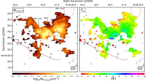
Figure 12: Propyne (CH₃CCH) physical parameters toward IRAS 16562$-$3959. Left and right panels show the column density and excitation temperature, respectively. We show in each panel the location of the NW cloud, the N-red cloud, the NEC-wall, the Diffuse Ridge, the position of DR (a), (b), and (c) (black crosses); and continuum sources 8 and 10 (red crosses).

Figure 12 shows the results of the fitting to the CH₃CCH lines. Uncertainties are shown in Figure B.1. Both the excitation temperature and column densities are consistent with previous single dish observations of the $5,K\shortrightarrow 4,K$ lines by Miettinen et al. (2006). They found a temperature of $35.9$ K and a column density of $1.5\times 10^{15}$ cm^-2 toward IRAS 16562$-$3959, which was the largest among their sample of 15 high-mass clumps. In general, we find the propyne column densities consistent with that given by Miettinen et al. (2006).

As shown in Figure 3 and described in Section 3.5.2, CH₃CCH is not particularly intense toward the CC core. Regions north of CC core and C8 are associated with the highest column densities of $\approx 2\times 10^{15}$ cm^-2. These regions are associated with temperatures of typically $60\text{--}65\pm 5$ K. The highest temperatures are $\gtrsim 85\pm 30$ K and they are detected toward low column densities regions. Generally, we detect warmer temperatures to the center of the clump than toward the outskirts. Averaging the CH₃CCH temperature in annuli of $2\arcsec$ starting from G345.49+1.47 we find that the radial temperature profile is well characterized by a decaying power law given by $80~{}\text{K}(r/0.01\text{ pc})^{-0.3}$. This temperature dependance is shallower than the one suggested for the dust temperature by Guzmán et al. (2010, $\propto r^{-0.4}$), which may reflect dust and gas requiring densities above $10^{5}$ cm^-3 to be thermally coupled.

Our results are in general agreement with what other studies have found toward high-mass star forming regions. Gibb et al. (2000), using single dish data taken toward the HMC G327.3$-$0.6, determined CH₃CCH temperatures of $72$ K and column densities of $2.9\times 10^{15}$ cm^-2, respectively. Therefore, they suggest that this hydrocarbon better traces the warm, extended component rather than the hot gas. Based on the rotational temperatures derived toward seven HMYSOs, Bisschop et al. (2007) classified propyne as a “cold” molecule. Interferometer studies toward three “organic poor” HMYSOs — which are expected to be younger and less chemically evolved than HMCs — indicate that CH₃CCH is as abundant far from the HMYSO as close to it, thus classifying it as an envelope molecule (Öberg et al., 2013; Fayolle et al., 2015). Propyne is also characterized by temperatures between 40–60 Kand, in NGC 7538 IRS9, by a temperature profile which roughly follows $\propto r^{-0.33}$..

Being an unsaturated hydrocarbon, there are in principle efficient ion-neutral gas formation routes for CH₃CCH (Schiff & Bohme, 1979). Concordantly, there is no evidence that in IRAS 16562$-$3959 the formation of a significant fraction of CH₃CCH has occurred in dust grains. First, the zero moment of all unsaturated molecules (except H₂CCO) including CH₃CCH are classified together within the Continuum group, consistent with ion-neutral gas reactions which tend to form unsaturated species. Second, let us assume that a large fraction of CH₃CCH is formed on dust grains and liberated afterwards to the gaseous phase. This would imply that CH₃CCH  should be well correlated with other molecules formed in grains, of which one of the best established examples is methanol. However, methanol emission does not correlate well with propyne as shown in Section 3.3. Finally, we note that the continuum correlates well with propyne in IRAS 16562$-$3959  and in other high-mass clumps (Giannetti et al., 2017). This is expected if its formation is dominated by gaseous ion-neutral reactions because these depend crucially on the high-energy ($\geq 100$ MeV) cosmic ray ionization, which is homogeneous throughout the clump (Herbst & Klemperer, 1973). That is, propyne’s abundance seems to depends more on the total column density of material rather than other circumstances like the presence of shocks, a higher temperature, or special illumination. We conclude that the good correlation of CH₃CCH with the rest of the unsaturated species and the continuum, as well as the lack of correlation with CH₃OH and with shock tracers like SiO, are consistent with the ion-neutral gas reactions forming a significant fraction of propyne in IRAS 16562$-$3959.

4.2 Column Densities and Excitation Temperatures

To determine excitation conditions and column densities we fit the molecular emission lines using simple models. It is possible to constrain the excitation state of species with several observed lines such as CH₃OH and CH₃CCH. Other molecules such as SO, SO₂, OCS, HNCO, C₂H₅CN, c-C₃H₂, HC₅N, CH₃C₃N, C₂H₃CN, and NH₂D also have several transitions which help determining their excitation conditions, but these higher excitation lines are only detected toward specific sources. For the rest of the molecules we detect either only one transition or the observed lines are unsuitable for discerning the excitation conditions of the gas (e.g., CCH and H¹³CN).

The sources for which we model the emission spectra correspond to those features identified in Section 3.2. Spectra for each of the sources are obtained by taking the primary beam corrected intensity (in K) versus frequency either toward specific directions or spatially averaging the intensity in the solid angle of the source. Spatial integration can improve the signal-to-noise ratio of the spectra if the physical conditions of the gas in the integrated area do not vary too much and the identified feature form a coherent physical structure. Otherwise, spatial integration may complicate the interpretation of the spectra and even smear out faint lines.

Spectra of the following sources are analyzed:

• CC core. Its spectrum is taken toward the peak methanol position, that is, $0\farcs 7$ in the $\text{P.A.}=-64\arcdeg 3$ direction from G345.49+1.47. Emission from this position avoids most of the red-shifted core nearby (see Section 3.2).

• C8. We judge C8 not being a completely coherent structure, with significant differences between positions closer to Source 8 and those closer to the maser a. Hence, we split the emission in two sources: a 1$\farcs$5 radius circular region around Source 8 and the maser a position.

• N-red cloud. We spatially average the emission in the region marked in Figure 7.

• NW-cloud. We spatially average the ellipse marked in Figure 7. Because this source is rather large, in order not to fade out some weak lines we also take the spectrum toward the position marked with NW(a) in Figure 7. NW(a) correspond to the peak position of methanol $2_{1,1}\shortrightarrow 1_{1,0}$ in the NW-cloud.

• NEC-wall. Toward this source we consider the spectra in two locations corresponding to the methanol and sulfur monoxide peaks, marked in Figure 7 with NEC-w(a) and NEC-w(b), respectively.

• Diffuse Ridge. The Diffuse Ridge is a much more elongated feature with varying characteristics along its extension. The size of the Diffuse Ridge also means it is likely affected by short baseline filtering. We select three positions to analyze the Diffuse Ridge, marked from (a) to (c) in Figure 7. Positions DR(b) and DR(c) correspond to the location of two cores in the Diffuse Ridge which have counterparts in several molecules. DR(a) is located on more diffuse gas forming the body of this ridge or filament.

We model the emission of all molecules except CH₃OH using a single excitation temperature (SET) model (van der Tak, 2011), that is, we assume one excitation temperature per line of sight. Due to the many detected lines of CH₃OH and because they are usually affected by non-LTE excitation, we model its emission using Radex (van der Tak et al., 2007). We assume, unless explicitly stated, that the beam filling factor of the emission is 1. Therefore, derived column densities are beam-averaged. Of course, in the cases of extended sources with spatially averaged spectra (e.g., the N-red cloud) these are source-averaged. For the line profiles, we model them as Gaussians with a single central velocity ($V_{\rm LSR}$) and FWHM ($\Delta V$) for all transitions from a specific molecule. We stress that due to the Hanning smoothing of the ALMA data, the effective spectral resolution is $976$ kHz. That is, the instrumental broadening amounts to $\approx 3.0$ km s^-1. In the SET model, the excitation temperature ($T_{\text{ex}}$), column density ($N$), $V_{\rm LSR}$, and $\Delta V$ are free parameters. For methanol, free parameters are $T_{K}$, the column density, $V_{\rm LSR}$, $\Delta V$, and density of the main collision partner (assumed H₂). For simplicity, we assume equal abundances of the E- and A-CH₃OH symmetry states because the kinetic temperature (Section 4.1) is always larger than the 7.9 K energy difference (in $k_{B}$ units) between the ground states of E- and A-CH₃OH (Friberg et al., 1988). The use of Radex for other molecules is hindered by the detection of only one or two transitions, which makes the modeling unreliable. We find optimal parameters by minimizing the squared difference between the data and the model, weighted by $\sigma^{-2}$, where $\sigma$ is the uncertainty of the primary beam corrected data (in K). Typical $\sigma$ for single pixel spectra (that is, not for spatially integrated) ranges in $0.04$–$0.06$ K. To minimize and calculate formal uncertainties we use Minuit and follow the prescription in Lampton et al. (1976). Tables 4 and 5 and Figures C.1 to C.13 show the results of the SET and Radex modeling.

Table 4 shows the results of the Radex modeling of the CH₃OH lines. Columns (1) to (5) indicate the source, $T_{K}$, the logarithm of the column density in cm^-2 ($\log\left(N\right)$), $V_{\rm LSR}$, $\Delta V$, and H₂ density, respectively. Column (6) remarks some noticeable characteristics of the fittings or of the data. For some sources (NEC-wall, C8, and NW-cloud) we exclude from the fitting the CH₃OH, ${\rm(E_{2})}$ $J_{K_{a}K_{c}}=5_{-1,0}\shortrightarrow 4_{0,0}$ maser transition because this strong, non-thermal line would require opacities $<-1$. These are characteristic of strong masers and cannot be adequately modeled by Radex (van der Tak et al., 2007). In other sources, for example toward the CC core, lines are well modeled assuming LTE conditions, which implies a lower bound on the density. According to Radex, densities $\gtrsim 10^{10}$ cm^-3 are needed to thermalize the masering ${\rm(E_{2})}$ $J_{K_{a}K_{c}}=5_{-1,0}\shortrightarrow 4_{0,0}$ line. Densities $\geq 10^{7}$ cm^-3 are usually enough to thermalize the rest of the observed methanol transitions. For those sources in which all methanol lines are thermalized except the ${\rm(E_{2})}$ $J_{K_{a}K_{c}}=5_{-1,0}\shortrightarrow 4_{0,0}$ we give a range of compatible densities.

Comparing the ${\rm(E_{2})}$ $J_{K_{a}K_{c}}=5_{-1,0}\shortrightarrow 4_{0,0}$ maser transition with the expected LTE intensities is useful to confirm the strong non-LTE effects on these lines. The maser spots a, b, and c identified in Figure 10 and whose parameters are given in Table 3 are associated with antenna temperatures between 200 and 400 K. These values are larger than the expected LTE emission by factors of 200, 1300, and 200, respectively. Assuming the angular size of the maser emitting regions covers less than a third of the beam size we obtain brightness temperatures ranging between 1500 and 3000 K. In addition, the linewidths of masers a and c given in Table 3 are also slightly narrower by $\approx 0.6$ than the linewidths of the rest of the CH₃OH lines, which is also a characteristic of masers. The CH₃OH, ${\rm(E_{2})}$ $J_{K_{a}K_{c}}=5_{-1,0}\shortrightarrow 4_{0,0}$ line corresponds to a class I maser, that is, it is collisionally excited followed by spontaneous radiative decay (Cragg et al., 1992). These are the first class I methanol masers detected toward IRAS 16562$-$3959; the only CH₃OH maser detected previously is the class II (radiatively excited) 6.7 GHz maser MMB345.498+1.467 (Caswell, 2009) detected toward Source 18. We note that the CH₃OH class II maser is not associated with the most luminous source G345.49+1.47, but with the apparently more evolved and less embedded Source 18. In fact, neither class I nor II CH₃OH masers are associated directly with G345.49+1.47, but they appear scattered throughout the clump. This is also the case for the masers observed toward IRAS 16547$-$4247 (including the ${\rm(E_{2})}$ $J_{K_{a}K_{c}}=5_{-1,0}\shortrightarrow 4_{0,0}$ transition), another clump believed to be in a similar evolutionary stage as IRAS 16562$-$3959 (Voronkov et al., 2006). Interestingly, for both clumps, not the methanol but the OH masers are associated with the central dominating HMYSO.

Table 5 shows the best-fit SET parameters for the rest of the molecules toward each source. Columns (1) to (5) indicate the molecule, $T_{\text{ex}}$ ($T_{K}$ for CH₃OH), $\log\left(N\right)$, $V_{\rm LSR}$, and $\Delta V$, respectively. In general, the $V_{\rm LSR}$ of different molecules are not the same and it is not rare to find differences of $\sim 3$ km s^-1 or more between different molecules for the same line of sight. For several sources, it is possible to gather together sets of molecules which share similar velocities. Column (6) in Table 5 identifies the number of the group to which each particular molecule belongs. Considering the limited velocity resolution of the data, two groups are sufficient to account for the $V_{\rm LSR}$ variations in each source. As a criterion for separating the two groups of $V_{\rm LSR}$, we require the internal standard deviation of each group being less than half of the standard deviation of the set of all the $V_{\rm LSR}$ of the source. We find that two groups describe adequately the $V_{\rm LSR}$ distribution of the CC core, the N-red cloud, the NEC-wall(b), DR(b), the NW cloud, and of the NW(a). For the rest of the sources, they are either well characterized by a single $V_{\rm LSR}$ or the velocities have a large dispersion which cannot be grouped in two well differentiated sets.

Table 5 gives formal uncertainties for the best-fit parameters, except for those which have been assumed or kept fixed during the minimization. Note that most of the $T_{\text{ex}}$ are assumed for the SET fitting in Table 5. The procedure to assign the assumed $T_{\text{ex}}$ for each molecule start with molecules for which it is possible to derive a temperature (generally CH₃OH, CH₃CCH, and SO). The CH₃OH and CH₃CCH temperatures are estimators of the kinetic temperature of the gas. SO, on the other hand, is associated with rather low $T_{\text{ex}}\leq 20$ and thus it is likely sub-thermally excited. In most cases, the assumed temperature for molecules without an independent $T_{\text{ex}}$ determination is one of these three.

In order to assign a sensible $T_{\text{ex}}$ to molecules for which an independent temperature estimation is not possible, we first check its $V_{\rm LSR}$ group. Two molecules having very different $V_{\rm LSR}$ is evidence that they trace different gas and, therefore, assuming the same $T_{\text{ex}}$ is not justified. In addition, we asses the critical densities associated with the lines. Considering that the critical density of the detected SO transitions ranges between $1.6$–$2.9\times 10^{5}$ cm^-3, we assign the same temperature as SO to all molecules whose transitions have critical densities above or equal to that of SO, that is, to HC₃N, HNCO, SiO, CCH, HCN, CS, and to their isotopologues. An exception to this rule occurs when the derived CS peak optical depth — assuming $T_{\text{ex}}$ from SO — is above 2. Because the CS, $J=2\shortrightarrow 1$ line has a similar critical density as SO, high optical depths could reduce the effective critical density and bring the CS line closer to LTE due to radiative trapping (Shirley, 2015). We assume that molecules with transitions associated with critical densities lower than that of SO (like H¹³CO⁺, NH₂D, HCS⁺, and OCS) are closer to LTE, and therefore, we use either the CH₃OH or CH₃CCH derived $T_{\text{ex}}$, depending on which one is closer in $V_{\rm LSR}$. We use CH₃OH or CH₃CCH temperatures for molecules without collisional excitation parameters (like several COMs) and in the case SO is not detected.

Column (7) gives additional information about the fitting and noticeable characteristics of the spectra, for example, whether the line has absorption features or if it is associated with high optical depths. In Table 5, the $T_{\text{ex}}$ entries which have not been derived from the fit have a superscript (^†, ^‡, or ${}^{{{\dagger}\!{\dagger}}}$). This marker indicates the origin of the assumed temperature for the SET fitting: the same marker appears in column (7) of the molecule from which $T_{\text{ex}}$ was adopted. In a few cases and lacking a better alternative, we also indicate whether we use $T_{\text{ex}}$ from a molecule within a different velocity group or from another source.

Note that Table 5 includes the CH₃OH parameters of Sources 3 and 18. Source 3 is a continuum source with a spectral index characteristic of dust emission (Paper I). The CH₃OH fitting is of a rather discrete quality, but we emphasize that this is one of the few lines of sight with emission in the transition . Source 18 was identified in Paper I as an HC Hii region associated with a HMYSO less massive than G345.49+1.47. Toward Source 18 we detect CH₃OH lines including high energy ($E_{\rm up}>100$ K) transitions. Source 18 is one of the uncommon cases of a relatively isolated continuum source with an unambiguous line counterpart and thus a YSO with a reliable $V_{\rm LSR}$.

Figures C.1 to C.13 (appendix C) show the SET and Radex best-fit models and the spectra in primary beam corrected K versus frequency. Individual panels show usually one transition each, but some panels show a few closely spaced lines (e.g., for CH₃CCH) of the same molecule. The name of the molecule and the upper energy level of the transition are displayed on top and in the top left corner of each panel, respectively. Models and data are shown in red and black, respectively. The green bar indicates the frequency range used to calculate the squared difference between data and model. Some panels with faint detections show the $\pm 2.5\sigma$ level, where $\sigma$ depends on the specific spectrum and it is given in the caption.

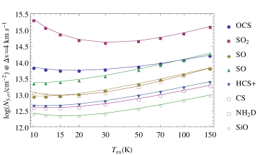
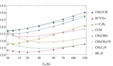
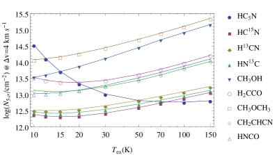
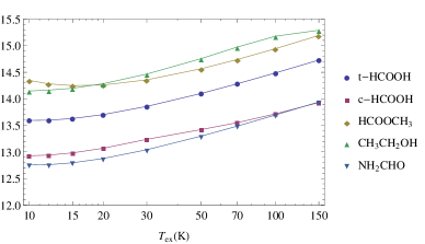
Figure 13: Each curve shows the minimum column density necessary to produce a Gaussian line peak of $5\sigma\approx 0.3~{}\text{K}$ and $\text{FWHM}=4$ km s^-1, in at least one transition in our spectral coverage, versus the excitation temperature (assuming LTE).

Finally, we emphasize that the lack of a molecule entry for a specific source in Table 5 is due to non-detection. The exception are the sulfur oxides for the CC core (SO, SO₂, and isotopologues), which are not present in the table because their spectra were analyzed in detail in Paper I and their emission cannot be well fitted by a single temperature model. The general criterion to discard a detection is the absence of any line attributable to the molecule over $2.5\sigma$ at a $V_{\rm LSR}$ between $-5$ and $-20$ km s^-1. However, in some cases detection of the main isotopologue of a species lends credibility to fainter spectral features located at the same $V_{\rm LSR}$. The non-detections are judged upon visual inspection of the spectra in the positions where the strongest lines are expected. Figure 13 shows the minimum column density needed to produce a Gaussian peak of $2.5\sigma\approx 0.143$ K with $\Delta V=4.0$ km s^-1 versus temperature, assuming LTE conditions for different molecules. This $\Delta V$ is typical of high-mass star formation regions but, in any case, the diagrams are easily scalable to other values because the peak of optically thin lines are proportional to the column density and inversely proportional to $\Delta V$. Figure 13 includes the minimum column density of some species typical of hot-cores which are not (or only dubiously) detected in this work.

5 FRACTIONATION AND ISOMERIZATION IN IRAS 16562$-$3959

The isotopic composition of molecular gas — presumably preserved until the beginning of further stellar nucleosynthesis — is a relevant initial condition of star formation. Deriving the proportions from molecular isotopologue ratios is not trivial, and entails determining what are the mechanisms that produce molecular fractionation. Because these mechanisms are sensitive to the present and past conditions of the molecular gas, characterizing them could in turn provide us with important constrains about the physical parameters of the clump (like the gas temperature).

Using the data presented in this work, we can study the fractionation of the following groups of isotopologues: SiO, ²⁹SiO, and ³⁰SiO; HC¹⁵N and H¹³CN; H¹³CO⁺ and HC¹⁸O⁺; ³⁴SO, SO, and ³³SO; CS, and C³³S; OCS and O¹³CS; and CH₃OH and ¹³CH₃OH. In addition to these, we study the H¹³CN/HN¹³C isotopomer fractionation. In principle, we can asses the silicon, sulfur, and carbon fractionations more directly because the isotopic difference between the molecules involve only one atom. On the other hand, for hydrogen cyanide and formylium the differences between the observed isotopologues involve two isotopes from different elements, complicating somewhat the interpretation.

The following sections present the analysis of the isotopic and isomeric fractionation toward IRAS 16562$-$3959. Table 7 shows a summary of the typical observed fractionations. Emission from the SiO, HCO⁺, and HCN isomers is extended, hence, Table 7 gives the average fractionation ratios measured toward the clump. The rest of the ratios characterize emission arising from the central core.

The isotopic proportion of many atoms are found to vary with Galactocentric radius (Wilson, 1999).We use $6.9$ kpc as the kinematic distance from IRAS 16562$-$3959 to the center of the Galaxy. Throughout this section we use square parentheses to represent abundances.

5.1 Silicon Fractionation

SiO and ²⁹SiO have been observed toward IRAS 16562$-$3959 using the SEST telescope by Harju et al. (1998) and Miettinen et al. (2006). The observed lines profiles are symmetric, with large wings (FWZP$=27.3$ km s^-1, Harju et al., 1998). Excitation temperatures reported by Miettinen et al. (2006) are typically $4.3\pm 0.1$ K, derived from simultaneous observations of the $3\shortrightarrow 2$ transition.

The velocity integrated emission from the $2\shortrightarrow 1$ lines reported in the literature toward IRAS 16562$-$3959 are $5.3\pm 0.1$ and $0.35\pm 0.3$ K km s^-1 for SiO and ²⁹SiO, respectively. Their ratio, $15.1$, is lower than the solar abundance value of $19.7$ (Asplund et al., 2009). It is also lower than the mean ratio found recently by Monson et al. (2017) of [SiO]/[²⁹SiO]=$17.9\pm 1.1$, who also argue for the lack of a Galactic gradient in the silicon isotopic distribution. The isotopic ratio varies within an interquartile range of $[9.6,17.2]$ (Table 7), but with no evident systematic spatial trend. Line ratios lower than the expected isotopic abundance proportion are usually interpreted as evidence of optically thick emission, which probably characterizes the main isotopologue (²⁸SiO) lines (Penzias, 1981). Optical depth introduces an additional complication, because its effects and abundance changes are in principle degenerate (the study by Monson et al., 2017 models the opacity broadening of the line to estimate $\tau$ independently).

From our ALMA data, we find line ratios between SiO and ²⁹SiO ranging between $9.2$ and $13.6$ (interquartile range), with a median value across the clump of $11.2$. We integrated the line emission in the same velocity range for each line ($-24$ to $0$ km s^-1) to calculate these values, but we note that using the zero moment maps (obtained through moment masking) gives similar results. The ratios we obtain are comparable to the ratios calculated by Monson et al. (2017) toward clouds in the central molecular zone of the Galaxy. Monson et al. do not attribute these low values to fractionation, but explain them as due to optical depths $\gtrsim 1$. This is likely only part of the explanation for the values obtained for IRAS 16562$-$3959. We observe that the SiO/²⁹SiO line ratio increases to a median value of $13.7$ if we integrate the lines away from the central $V_{\rm LSR}$. Presumably, emission from the line wings is more likely associated with optically thin column densities. However, the proportion is still low compared with the mean Galactic value. Because it is also possible that the main isotopologue line being affected by short spacing losses, we refrain from attributing the low [SiO]/[²⁹SiO] line ratios to fractionation.

We derive ²⁹SiO column densities toward the N-red cloud, the S8 maser position, the NW cloud, and position (a) from the NW cloud, and found [SiO]/[²⁹SiO] values of, respectively, $14.8\pm 1.0$, $19.5\pm 2.0$, $18.6\pm 2.3$, and $12.3\pm 1.7$, where the error bars represent formal uncertainties. These values are somewhat higher that those obtained from the zero moment maps. It may be possible that, because they are associated with emission from rather compact sources, they could be less affected by short spacing losses. It is apparent that a fair assessment of the SiO fractionation toward IRAS 16562$-$3959 entails observing the likely optically thin line wings with an adequate short spacing coverage.

We expect the ²⁹SiO and ³⁰SiO emission to have opacities lower than those of the main isotopologue, and also being less affected by short baseline filtering. Indeed, the ²⁹SiO/³⁰SiO velocity integrated line ratios are distributed within an interquartile range of $[1.2,1.6]$ and a median of $1.4$. This value is the same as the median ratio obtained by Monson et al. (2017), and it is very similar to the solar value ($1.5$, Asplund et al., 2009). We also derive ³⁰SiO column densities toward the N-red cloud, the S8 maser position, and the NW cloud, observing little variation: we obtain [²⁹SiO]/[³⁰SiO] values of $1.5\pm 0.1$, $1.2\pm 0.1$, and $1.4\pm 0.26$, respectively.

Finally, we emphasize that we do not find obvious spatial trend or pattern in the distribution of any of the SiO isotopologue ratios. This is in line with what is found by Monson et al. (2017). Because the origin of SiO in the gas phase is likely dust sputtering in shocks, it is unlikely that this mechanism be sensitive to the rather small relative difference between the molecular masses of the SiO isotopologues. Furthermore, any chemical mechanisms affecting the SiO relative isotopic abundance in the clump probably act on timescales larger than the depletion time of SiO onto dust grains, therefore, not generating detectable fractionation.

5.2 Sulfur Fractionation

In this section we analyze the relative abundances of the sulfur isotopologues ³²S (main), ³⁴S and ³³S. The only source toward which we claim detection of ³³SO is the CC core. Assuming an excitation temperature of $64$ K, the ³⁴SO column density toward the CC core is $9.3\pm 0.2\times 10^{14}$ cm^-2. Combining this with the ³³SO column density given in Table 5, we obtain [³⁴SO]/[³³SO]$=5.4\pm 0.6$. This value is remarkably close to the solar isotopic proportion [³⁴S]/[³³S]$=5.64$ (Asplund et al., 2009). The analysis of Paper I also indicated that the ³⁴SO abundance respect to the main isotopologue (³²SO) was consistent with solar abundance. Note that the isotopic proportions of sulfur are predicted to vary little with Galactic radius (Chin et al., 1996): at $6.9$ kpc, the expected [S]/[³⁴S]$=27\pm 5$ is still consistent with the solar abundance ratio. We conclude that, toward the central HMC, the isotopic abundances of sulfur — from SO emission lines — are consistent with the solar value. We refrain from analyzing the [CS]/[C³³S] ratio because in the directions where we detect C³³S, the CS line is optically thick.

5.3 Carbon Fractionation

We can compare the abundance of ¹³C-bearing molecules with their main isotopologue using lines from O¹³CS, ¹³CH₃OH, and HC¹³CCN. We avoid using the lines of H¹³CCCN and HCC¹³CN because they are blended with lines of HNCO and C₂H₃CN, .

O¹³CS and ¹³CH₃OH are only detected toward the CC core. Using the column densities of Table 5, we obtain [OCS]/[O¹³CS]$=25\pm 2.4$, assuming the same excitation temperature for both molecules. This ratio is below the expected value for [C]/[¹³C]$\sim 60$ (Wilson, 1999; Milam et al., 2005) and it is similar to the values found by Tercero et al. (2010) toward Orion-KL. The most likely cause for this difference is that the OCS line is optically thick. LTE fittings with derived column densities compatible with the solar isotopic abundances require peak optical depth ($\tau_{p}$) of $1.65$, filling factors $\lesssim 0.3$, and excitation temperatures higher than $100$ K.

The isotopologue ratio calculated from the methanol column densities gives [CH₃OH]/[¹³CH₃OH]$=26\pm 4$. This number is comparable to the one obtained above using OCS, and it is a factor of $\sim 2$ less than the values derived for Orion by Persson et al. (2007). Similarly as in the case of OCS, LTE column densities derived for an optically thick CH₃OH line ($\tau_{p}\approx 2$ for the ${\rm(E_{2})}$ $J_{K_{a}K_{c}}=5_{-1,0}\shortrightarrow 4_{0,0}$ transition) with a filling factor of $0.24$ give isotopic ratios $\sim 50$, closer to the expected [C]/[¹³C] value.

Finally, we can calculate the [HC₃N]/[HC¹³CCN] quotient toward the CC core, the NEC-wall positions (a) and (b), the C8 maser position, and the C8 1$\farcs$5 radius source. The ratios obtained from Table 5 for these five sources are $32\pm 4$, $41\pm 4$, $37\pm 5$, $60\pm 6$, and $50\pm 4$, respectively. The error bars give the formal uncertainty, but there is a likely more relevant systematic uncertainty associated with the excitation temperature. Note that because we only detect one line for each isotopologue, the assumed excitation temperature is critical. The ratio obtained for the CC core emission is close to the values obtained for O¹³CS and ¹³CH₃OH. Again, the column density quotient between the two isotopologues can accommodate a value closer to $50$ if the opacity near the peak of the HC₃N line is $1.9$ and the filling factor $\lesssim 0.5$. The ratios increase with distance from the center of IRAS 16562$-$3959: from the CC core to the NEC-wall, reaching values consistent with the expected isotopic ¹³C abundance for the C8 sources. This is consistent with the view that quotients lower than the expected isotopic abundance ratio are caused by opacity.

5.4 Formylium Cation: Oxygen and Carbon Fractionation

The median value we calculate for the velocity integrated flux ratio between H¹³CO⁺ and HC¹⁸O⁺, within the range $-15~{}\mbox{km~{}s${}^{-1}$}<V_{\rm LSR}<-9~{}\mbox{km~{}s${}^{-1}$}$, is 6.9, with an interquartile range of [4.8, 8.5]. This abundance ratio depend on carbon and oxygen isotopic abundances, which at the clump’s location are [¹²C]/[¹³C]=$59.4\pm 18$ and [¹⁶O]/[¹⁸O]=$442.8\pm 116$, respectively (Wilson, 1999). We infer that [H¹³CO⁺]/[HC¹⁸O⁺]=$7.5\pm 3.0$. Using instead [¹²C]/[¹³C]=$63.4$ (Milam et al., 2005) we obtain [H¹³CO⁺]/[HC¹⁸O⁺]=$7.0$, which is within the previous value uncertainty. The median value found toward IRAS 16562$-$3959 is remarkably close to expected ratio, considering the uncertainties.

However, in contrast to the SiO isotopologue, we do see a systematic trend in the H¹³CO⁺/HC¹⁸O⁺ line ratios: the central parts of IRAS 16562$-$3959 (within 12″ from G345.49+1.47) are associated with ratios higher than average, with a mean value of $\sim 8.5$. Regions farther away from the center of the clump, like the emission associated with Sources 7 , 3 , and 2 (the Continuum arc) and to sources in south east like 15 and 17; exhibit ratios $\sim 5$. This behavior of the line ratios is rather surprising because it is the opposite to what would be expected if the lines from the central parts of IRAS 16562$-$3959 are optically thick. In principle, short spacing losses could affect the line ratios, but they would not explain the spatial differences.

Short spacing observations are needed to confirm whether the effect is real or due to filtering. Additionally, HCO⁺ observations would determine whether the cause of this decrement is fractionation, and of which isotopologue. Finally, we mention a possible path to increase the H¹³CO⁺ abundance near the center of the clump respect to HC¹⁸O⁺: it may merely reflect ¹³CO being better (self) shielded than C¹⁸O from radiation arising from G345.49+1.47, simply because of the lower abundance of the latter. We note that the HMYSO has contracted and its high energy radiation has already ionized a small region in the center of IRAS 16562$-$3959. If HCO⁺ is formed mainly by combining H${}_{3}^{+}$ and CO, an increase of ¹³CO respect to C¹⁸O could produce a corresponding increase in the formylium isotopologue.

5.5 Hydrogen Cyanide: Nitrogen and Carbon Fractionation

Figure 14 shows in the left panel the quotient between the moment zero images of the H¹³CN and HC¹⁵N, $J=0\shortrightarrow 1$ transitions. These two molecules have different C and N isotopes, which means that their quotient depends on the fractionation of these two atoms. In practice, because of the better knowledge about the C vs. ¹³C proportion and because HCN transitions are usually optically thick, the [H¹³CN]/[HC¹⁵N] ratio is commonly used to study the N vs. ¹⁵N fractionation. Single dish observations of IRAS 16562$-$3959 of the same isotopologue pair studied in this section were performed by Dahmen et al. (1995).

There has been some discrepancy in the literature respect to the [N]/[¹⁵N] behavior with Galactocentric radius. While Wilson (1999) — based on H¹³CN and HC¹⁵N observations from Dahmen et al. (1995) and Wannier et al. (1981) — suggests a value of $420$ at the distance of IRAS 16562$-$3959, Adande & Ziurys (2012), based on HNC and CN observations, proposes a lower value of $270$. The latter authors suggest that the difference is due to the assumed [C]/[¹³C] curves (illustrating the uncertainties introduced by the double isotope corrections) but this is not clear since there are already noticeable differences between their [HN¹³C]/[H¹⁵NC] and the [H¹³CN]/[HC¹⁵N] values given by Dahmen et al. (1995). In view of these uncertainties, we focus the quantitative analysis directly on the [H¹³CN]/[HC¹⁵N] ratio.

According to the image shown in Figure 14, the mean H¹³CN/HC¹⁵N line quotient (which is the same as [H¹³CN]/[HC¹⁵N], assuming the same excitation temperature for both molecules) rises from values $\sim 3.5$ near G345.49+1.47, to typically $4.0$ at 10″ from the center of IRAS 16562$-$3959. At these distances from the clump center, the behavior of the quotient is dominated by the values obtained near the CC core, the NEC-wall and the C8. Farther away from the HMYSO, the mean ratio has a slightly steeper rise to reach values between $5.5$ and $6.0$ at 25″ from the clump center. These values are dominated by the higher quotients measured toward the Diffuse ridge and the NW cloud. The values obtained for [H¹³CN]/[HC¹⁵N] from the LTE fittings (Table 5) for each source are similar to those read from Figure 14. The mean [H¹³CN]/[HC¹⁵N] is $5.7\pm 2$, where the uncertainty represents the dispersion observed between different sources. This value is slightly lower, although within the uncertainties, compared with that given recently by Colzi et al. (2018) at 6.9 kpc.

Using single dish data, Dahmen et al. (1995) obtained [H¹³CN]/[HC¹⁵N]$=6.32\pm 0.16$ for IRAS 16562$-$3959. It is not clear that the lower ratios obtained for the sources close to the center of IRAS 16562$-$3959 are compatible with this value using optically thick lines. For example, the ratio of 3.5 obtained for the CC core is consistent with the value found by Dahmen et al. (1995) only if the H¹³CN line is associated with an optical depth at peak of $\sim 4$. Such high opacity would affect the observed relative intensities of the hyperfine components, deteriorating noticeably the quality of the fits: we do not observe in general large hyperfine anomalies which could be evidence of an optically thick H¹³CN line. It is still not clear how much influence the short baseline filtering has on the line quotients, but at least for the CC core, it is not likely to dominate.

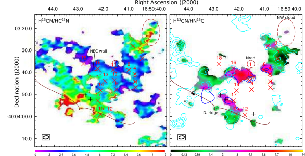
Figure 14: Left panel. Moment zero quotient between the H¹³CN and HC¹⁵N, $J=0\shortrightarrow 1$ transitions. Right panel. Moment zero quotient between the H¹³CN and HN¹³C, $J=0\shortrightarrow 1$ transitions. Blue contours are drawn at the 25, 50, and 75% of the peak H¹³CN moment 0 emission. Cyan contours correspond to NH₂D emission as in Figure 15. In both panels we indicate the N-red, NW- and Diffuse ridge markers as in Figure 7.

Hence, it is possible that there is real fractionation effect toward the densest cores of IRAS 16562$-$3959. Measurements of the [H¹³CN]/[HC¹⁵N] show that this proportion varies depending on the nature of the source. For example, Wampfler et al. (2014) finds that the quotients associated with three low mass protostellar envelopes are $2.4$, $4.2$, and $5.3$. The causes for the different values are not entirely clear, but the lowest ratio (highest HC¹⁵N fractionation) is associated with the hot corino IRAS 16293$-$2422 A. The latter source is somewhat colder and less affected by external illumination compared with the other two. Guzmán et al. (2015b, 2017) have also determined very low ratios ($\leq 3.0$) toward proto-planetary disks. Of the two fractionation mechanisms suggested by Guzmán et al. (2015b), one of them only acts effectively in cold gas ($\leq 20$ K), which is not characteristic of IRAS 16562$-$3959. The other, selective photo-dissociation (closely related with self-shielding, Heays et al., 2014), predicts that the [N]/[¹⁵N] ratio should increase the more illuminated with dissociating radiation and diffuse a cloud is. In this case, the same self-shielding from the HMYSO radiation which may cause the H¹³CO⁺-HC¹⁸O⁺ spatial fractionation could also explain the observed [H¹³CN]/[HC¹⁵N] ratios.

5.6 H${}^{\textit{13}}$​CN/HN${}^{\textit{13}}$​C Isomer Ratio

We can explore the HCN to HNC isomer ratio in IRAS 16562$-$3959 using their ¹³C isotopologues, whose transitions have the advantage of being more likely optically thin compared to those of the main species. The HCN/HNC ratio has been found to depend on kinetic temperature (e.g., Schilke et al., 1992). Theory proposes that the two molecules are produced in a ratio $\sim 1$ mostly through dissociative recombination of HCNH⁺ (Herbst, 1978; Hirota et al., 1998). Selective destruction of HNC through the neutral-neutral reaction $\text{HNC}+\text{H}\rightarrow\text{HCN}+\text{H}$ is expected to work at higher temperatures because of the presence of an activation barrier, depleting HNC in favor of HCN. The question of what is the energy of this activation barrier is still not completely resolved (Graninger et al., 2014).

The right panel of Figure 14 shows the quotient between the moment zero of the H¹³CN and HN¹³C, $1\shortrightarrow 0$ lines. This figure shows a qualitative correspondence with what is expected for the HCN/HNC ratio. Away from the center of IRAS 16562$-$3959 the temperatures are low and the H¹³CN/HN¹³C quotient is comparable to unity. Close to the center of IRAS 16562$-$3959 and to Source 8 the temperature is higher, the H¹³CN/HN¹³C quotient increases by one order of magnitude. It is also apparent that the molecular ratio is higher in the NE side of the Diffuse ridge, being presumably illuminated and heated more directly by G345.49+1.47. For the CC core, the column density given in Table 5 compared with the upper limits from Figure 13 suggests a ratio $\sim 100$. Regions where we detect NH₂D in combination with HN¹³C, the H¹³CN/HN¹³C ratios have values close to unity, again consistent with the low temperatures expected to be traced by deuterated species (Bergin & Tafalla, 2007).

The right panel of Figure 14 shows the quotient between the moment zero of the H¹³CN and HN¹³C, $1\shortrightarrow 0$ lines. There are significant differences between the H¹³CN and the HN¹³C emission, the most noticeable in the moment zero map is the lack of a CC core counterpart in HN¹³C, in contrast to H¹³CN. In addition, it is not uncommon these lines having different $V_{\rm LSR}$, as shown for several sources in Table 5.

The differences can be understood as due to the depletion of HNC in favor of HCN in gas at temperatures $>25$ K, which implies that warmer gas along a given line of sight will weight more into the H¹³CN emission than HN¹³C. Arising from different locations, warm and cold gas do not necessarily share the same $V_{\rm LSR}$. This interpretation implies also that the effective temperature of the HCN emission should be higher than that of HNC (Jin et al., 2015). Conversely, low temperatures should be associated with HCN/HNC column density ratios close to unity, the same effective temperature for both species, and consistent $V_{\rm LSR}$.

6 DISCUSSION

We can gain some insight on the chemistry and physics of the clump by comparing ours with independent observations. In Section 6.1 we compare our ALMA with NIR data taken from the literature. The latter are some of the few data on IRAS 16562$-$3959 with comparable angular resolution and coverage. Finally, Section 6.2 analyzes in more detail and draw some conclusions about the possible chemical processes at work in IRAS 16562$-$3959.

6.1 Near-Infrared Counterparts of Molecular Features

Figure 15 shows a three color NIR image (JHK_S filters) of IRAS 16562$-$3959 using data from the VVV survey (Minniti et al., 2010). We have superimposed in the left and right panels contours of the zero moment CH₃OH and NH₂D maps, respectively. Guzmán et al. (2016) analyzed similar NIR images toward G345.49+1.47, describing among other features the illuminated blueshifted outflow cavity and some continuum sources with NIR counterparts. In this section we focus on the molecular emission counterparts.

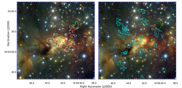
Figure 15: Both panels show in the background three color NIR images (red, green, and blue for K_s, H, and J band filters, respectively) obtained from the VVV survey. Left panel. White contours show CH₃OH, $2_{1,1}\shortrightarrow 1_{1,0}$ zero moment emission. Levels: 10, 30, 50, 70, and 90% of the peak ($0.51$ Jy beam^-1 km s^-1). Right panel. Cyan contours show deuterated ammonia $(J,K)=(1,1)$ zero moment emission. Levels: 10, 30, 50, 70, and 90% of the peak ($0.10$ Jy beam^-1 km s^-1). Red crosses mark the continuum sources 2, 3, 7, 8, 10, and 12. Green-dashed ellipses show the location of the NW and N-red clouds, and the NEC-wall. Black crosses mark the DR(a), (b), and (c) positions.

There are three NIR conspicuous features which correlate with the CH₃OH zero moment emission. The most evident is the CC core, which is coincident with a NIR source associated with the HMYSO G345.49+1.47. As already noted before, the CC core emission extends a few arcseconds in the north and north-east directions respect to G345.49+1.47. The second feature is coincident with the northern wall of the blueshifted illuminated cavity, particularly, the strong CH₃OH emission associated with the NEC-wall. Additional methanol emission seems to follow the location of the southern wall of this cavity, although in a less clear way compared to the NEC-wall. The third feature is evident in the left panel of Figure 15, which shows that the Diffuse Ridge seen in the CH₃OH contours coincides with a dark filament seen across the brightly illuminated blueshifted outflow cavity. From the brightness decrement produced by the filament in the K_s image, which amounts to $A_{K_{s}}\approx 0.3$ magnitudes, we derive an H₂ column density of $1.8\times 10^{21}$ cm^-2 (Rieke & Lebofsky, 1985; Heiderman et al., 2010). The median $V_{\rm LSR}$ of the Diffuse Ridge is $-11.7$ km s^-1 (Section 4.2), which is redshifted respect to the CC core. A likely interpretation is that the Diffuse Ridge material is in front of the outflow cavity, obscuring the illuminated cavity, and possibly falling toward the clump.

The right panel of Figure 15 shows NH₂D contours against the NIR background. Also indicated in this panel are the positions of continuum Sources 1, 2, 3, 7, 15, and 16. We can see that Sources 2, 3, and 7 delineate what we called in Section 3 the Continuum Arc, which is also seen in NH₂D. The NIR image shows that the Continuum Arc is embedded within a large IR-dark absorption region. The absence of stars observed toward this area suggests large column densities. There is a less evident NIR counterpart to the NH₂D peak located in the northeast part of IRAS 16562$-$3959. The NH₂D emission corresponds with an absorption patch where we see only most likely foreground stars, evidenced by their blueish hue. The deuterated ammonia line peaks at $-15.1$ km s^-1 and has a FWHM of $\sim 4$ km s^-1. Note that the true linewidth is smaller and closer to $2$ km s^-1 due to the instrumental broadening (see Section 2).

The most clear NIR counterpart to the NH₂D emission is located to the southeast, coincident with a very clear IR-dark cloud $\sim 15\arcsec$ size. This IR-dark cloud was already noted by Guzmán et al. (2016) because it is located nearby the outer-eastern ionized lobe of the G345.49+1.47 jet. The spatial coincidence and the kinematics of the jet’s lobe suggest that the jet may be interacting with this cloud. Its NH₂D emission peaks at $-11.7$ km s^-1 with a FWHM of $4.5$ km s^-1, which implies that the dark cloud is indeed part of IRAS 16562$-$3959, supporting the previous interpretation.

IR-dark regions are usually associated with dense and cold starless gas (Rathborne et al., 2006). In the case of IRAS 16562$-$3959, the cold nature of the gas associated with the dark IR regions is corroborated by their association with NH₂D (Bergin & Tafalla, 2007) and by all the rest of the detected spectral features being in absorption. Lines of CS, CH₃CCH, CCH, H¹³CN, HN¹³C, and CH₃OH appear in absorption toward both the south and northeast NH₂D peak positions.

6.2 Chemistry in IRAS 16562$-$3959

Studying the chemistry of a single high-mass protostellar molecular clump is a complicated task since it encompass many of the mechanisms expected to be at work in the ISM. Until the recent advent of instruments such as ALMA the chemistry of high-mass protostellar clumps had been studied using single-dish telescopes. These mix different environments in their beams, having to rely on velocity differences to discern them. With high resolution and sensitive observations we are now able to study in detail these regions, and spatially separate the emission of each molecule. Such studies are very useful to advance our chemical knowledge.

Near the end of the prestellar stage, a high-mass molecular clump is characterized by temperatures $<15$ K, hydrogen column densities $\gtrsim 10^{22}$ cm^-2, and densities $\gtrsim 10^{4}$ cm^-3. These are the characteristics of the so-called quiescent infrared dark clouds (Guzmán et al., 2015a; Rathborne et al., 2006). In this stage, dust grains are covered by (mostly water) icy mantles together with other adsorbed atoms and molecules like H, CO, N₂, and possibly CS and H₂S (Viti et al., 2004). At these low temperatures, only H is mobile on the dust’s surface and it reacts with other molecules (like CO) using the dust grain as a third body which helps dissipating the excess energy. Chemical products formed in the dust grain icy layer during this stage are typically hydrogenated species like H₂CO and CH₃OH (Vasyunina et al., 2014). Meanwhile, the cold gas in the clump also evolves chemically, specially through ion-neutral and barrier-less neutral-neutral reactions. A permanent, small amount of cosmic-ray ionization facilitates the gaseous ion-neutral reactions and formation of simple unsaturated molecules.

At these early evolutionary stages, most of the molecules formed on dust grains remain there: the temperature is too low to sublimate them from the surface. About all of the ices will co-desorb with water when the temperature reaches $\approx 100$ K. However, even at low temperature several non-thermal mechanisms can help desorbing some of these products, e.g., shock sputtering, chemical desorption, and photo-desorption. Some of these mechanisms — not being entirely clear which one(s) — are observed to be efficient at releasing large quantities of CH₃OH during the prestellar phase (e.g., Sanhueza et al., 2013; ).

As the clump evolves, it contracts, and eventually young stars are born. These (HM)YSOs increase the clump’s temperature and introduce turbulence through outflows and winds. Temperature rising to $20$–$30$ K reduces the time spent by H in the surface of the grains, hampering further hydrogenation reactions. The temperature rise increases the mobility of heavier radicals in the mantles, allowing further reactions and promoting the formation of more complex molecules. This phase of chemical evolution receives the name of warm-up (Garrod et al., 2008). The radicals may be produced by photolysis of other molecules induced by secondary cosmic rays UV-photons. Some other species (CO, N₂, O₂, CH₄) desorb with the increasing temperature (Viti et al., 2004), potentially opening new chemical routes.

The third phase of chemical evolution comes only near the regions where the temperature increases to $\geq 100$ K, that is, very near the young stars and inside the HMCs. Here, the water ices completely evaporate and liberate all the molecules formed in the dust mantles to the gas phase. The temperature rise also allows reactions with barriers and endothermic reactions to occur. Characteristic chemical products generated during the three stages described above — cold prestellar, warm-up, and HMC — are called by Herbst & van Dishoeck (2009) zeroth-, first-, and second-generation species, respectively.

Note that the dominating chemical mechanism in each stage is mainly determined by the temperature of the gas, which ultimately depends on the distance to the young forming stars. Protostellar clumps, like IRAS 16562$-$3959, are expected to roughly follow the chemical timeline presented above. They should likewise display all these stages at the same time depending on the location of the material: cool pockets of starless “pristine” gas remain present until the clump is ultimately dispersed; warm, less dense gas presumably occupies most of the volume of the clump; and finally, hot gas in the immediate surrounding of YSOs displays the chemical signatures of HMCs. Following the processes and classification described above, we analyze in the next sections some aspects about the chemistry of IRAS 16562$-$3959.

6.2.1 HMCs and embedded YSOs

HMCs are defined observationally as dense ($>10^{7}$ cm^-3), warm (100–500 K), and compact ($<0.05$ pc) molecular cores (Allen et al., 2017). The definition is not strict and it has changed at the same time that telescopes resolve more compact and hotter components (van Dishoeck & Blake, 1998). A rich spectrum including molecular transitions of hot ammonia, water, and COMs like CH₃OH and CH₃CN signpost the presence of a HMC. In general, it is assumed that the heating source of a HMC is a HMYSO located near its center.

There are four compact continuum sources within IRAS 16562$-$3959 which are clearly associated with high excitation molecular emission: Sources 3, 8, 10, and 18. All of these are detected in CH₃OH lines. Source 3 is a continuum source associated with hot methanol ($T_{\text{ex}}\approx 200$ K) but no IR counterpart, which prompts us concluding that it correspond to a HMC associated with a very embedded YSO. Source 18, on the other hand, is conspicuous in IR (2MASS and Spitzer/IRAC bands) and it is associated with the high-to-intermediate mass YSO GLIMPSE G345.4977+01.4668 ($L_{\text{bol}}\approx 10^{4}\mbox{$L_{\sun}$}$, Benjamin et al., 2003). It is not clear that Source 18 is associated with a HMC because — being bright at NIR — the YSO cannot be very embedded. In addition, the CH₃OH  temperature ($64$ K) and column density ($5.7\pm 0.5\times 10^{15}$ cm^-2) are significantly lower than those of the rest of the HMCs.

Source 8 and 10 are associated with two molecular cores, respectively, C8 and the CC core. These cores are the richest sources of molecular lines in IRAS 16562$-$3959. The CC core is associated with temperatures $>100$ K and hydrogen saturated COMs, which are characteristic of HMCs. The heating source is the HMYSO G345.49+1.47, which ionizes an associated HC Hii region. It is natural to assume that this ionizing radiation will also dissociate a large fraction of molecules in the immediate surroundings of the HMYSO, thus, the molecular emission does not need to coincide exactly with the HMYSO position (e.g., Mookerjea et al., 2007). C8, on the other hand, is embedded in a dense molecular envelope which extends to the northwest. This envelope apparently engulfs the position of Maser a, which is associated with a previously unreported continuum source of $2.1$ mJy at 3 mm. Seemingly, Maser a pinpoints the location of another embedded YSO. C8 is also characterized by CH₃OH lines with $T_{\text{ex}}>100$ K and other COMs with $T_{\text{ex}}>70$ K revealing the presence of a HMC. In contrast to the CC core, no evidence of free-free emission is observed toward C8.

In order to contrast the chemical composition between the CC core and C8, we compare the abundances of several molecules respect to methanol. The main reason to derive methanol-normalized abundances is that the hydrogen column density toward the CC core is very difficult to estimate due to most of the 3 mm continuum corresponding to free-free emission arising from the HC Hii region. We focus first on the abundance of O- and N-bearing molecules, which is a rather common approach in the literature (e.g., Widicus Weaver & Friedel, 2012; Allen et al., 2017). This strategy is also justified because the only hydrocarbon COM (that is, without N or O), CH₃CCH, seems to trace the clump material on a large scale rather than gas associated with the molecular cores. Identifying the O- and N-bearing groups was originally motivated by observations of Orion-KL, which show that nitrogenated and oxygenated molecules are better associated with two distinct structures, respectively, the HMC and the compact ridge (Feng et al., 2015, and references therein). A thermal segregation is also observed, with N-bearing molecules tracing hotter gas compared to the O-bearing species (Crockett et al., 2015). N-O segregation has been found toward other high-mass star forming regions as well (Su et al., 2005; Öberg et al., 2013; Allen et al., 2017), but it does not seem to be universal (Fontani et al., 2007).

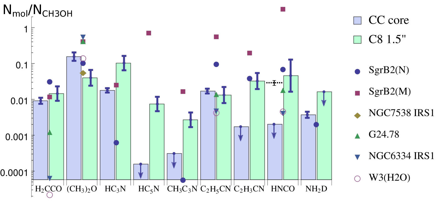
Figure 16: Blue and green bars show column density ratios for O- and N-bearing molecules more complex than four atoms toward the CC core and C8 (C8 1$\farcs$5), respectively. We use the values given in Table 5 for C8 1$\farcs$5 and the first velocity component toward the CC core. Error bars indicate formal uncertainties and arrows indicate lower bounds. We also show abundance ratios measured toward six HMCs from the literature (Sgr B2 sources from Belloche et al., 2013, NGC 7538 from Öberg et al., 2014, and the rest of the sources from Bisschop et al., 2007). The black dashed line and error bar indicate the [HNCO]/[CH₃OH] ratio obtained toward the CC core using the column density of HNCO given in Table 16 associated with the second velocity component.

Figure 16 compares the methanol-normalized abundance of O- and N-bearing molecules with four atoms or more, detected toward the CC core or C8 (thus excluding CH₃CHO). Figure 16 also shows abundance ratios associated with well-known HMC sources such as Sgr B2 (N) and (M) (Belloche et al., 2013), NGC 7538 IRS1 (Öberg et al., 2014), G24.78, NGC6334 IRS1, and W3(H₂O) (Bisschop et al., 2007). We note that the relative abundance ratio respect to CH₃OH for different sources can vary within several orders of magnitude, depending on the molecule. Part of this variation may be due to most values reported in Figure 16 are obtained from single dish telescope observations, which combines emission from several regions in the beam. Therefore, these ratios are useful only as rough estimations. In any case, the abundance ratios toward the CC core and C8 are comparable to those of other sources, within the observed variations.

The only molecule in Figure 16 more abundant in the CC core than in C8 respect to CH₃OH is CH₃OCH₃. We do not detect NH₂D toward C8, but its abundance upper limit is above the [NH₂D]/[CH₃OH] ratio measured toward the CC core. We measure the same abundances respect to methanol of C₂H₅CN and H₂CCO for both cores. For the rest of the molecules (HC₃N, HC₅N, HNCO, C₂H₃CN, and CH₃C₃N), we observe larger abundances toward C8 than toward the CC core. We add a note of caution about HNCO. Lines from this molecule toward the CC core are characterized by a $T_{\text{ex}}$ and $V_{\rm LSR}$ similar to those of CH₃CCH, hence they are not directly associated with the HMC. However, there seems to be in addition a hotter component, prompting us to conclude that the observed HNCO lines blend emission from the HMC and its colder envelope. We indicate in Figure 16 both the [CH₃OH]/[HNCO] lower limit and the ratio using the column density of Table 5.

There are two COMs more complex than CH₃OH detected toward both the CC core and C8: methoxymethane and propanenitrile (C₂H₅CN). These two molecules are representative of O-bearing and N-bearing COMs, respectively. The CH₃OCH₃ and C₂H₅CN lines toward C8 peak at the location of Source 8. Toward the CC core, they peak together with the highest energy CH₃OH transitions despite CH₃OCH₃ and C₂H₅CN lines coming from relatively low upper energy ($E_{\rm up}<40$ K) transitions. Similar to CH₃OH, a hotter CH₃OCH₃ component is blended in the CC core emission: the LTE fitting ($T_{\text{ex}}=138$ K) underpredicts the $16_{3,14}\shortrightarrow 15_{4,11}$ transition with $E_{\rm up}=136.6$ K.

Methoxymethane to methanol ratios of $1.7\pm 0.03\times 10^{-1}$ and $4\pm 2\times 10^{-2}$ are measured toward the CC core and C8, respectively. These ratios are within the values found toward most high-mass star forming clumps. The [CH₃OCH₃]/[CH₃OH] ratio does not vary much among different sources, which Öberg et al. (2014) interprets as evidence of CH₃OCH₃ forming on the ice mantles of dust grains and co-desorbing with CH₃OH. Compared with methanol, methoxymethane is slightly less abundant toward C8 compared to the CC core. In this regard, C8 is somewhat more consistent with colder ($<50$ K) sources (Öberg et al., 2014).

The [C₂H₅CN]/[CH₃OH] ratio shows a range wider than that of CH₃OCH₃ between different sources, from $\sim 10^{-3}$ in G35.03A (Allen et al., 2017) to $0.2$ in Orion-KL ‘D’ (Wright et al., 1996). Toward the CC core and C8 we measure the same ratio $[\mbox{C${}_{2}$H${}_{5}$CN}]/[\mbox{CH${}_{3}$OH}]\approx 1.6\times 10^{-2}$, which is consistent with other hot cores like G34.26+0.15SE (Mookerjea et al., 2007) and the sample of Bisschop et al. (2007) (see Figure 16). We do not detect clear evidence of thermal or spatial N-O COM segregation in either core. However, we note that at least in Orion-KL, CH₃CN shows the N-O segregation much more clearly than C₂H₅CN (Crockett et al., 2015).

We can explain some of the abundance differences shown in Figure 16 if C8 is chemically more evolved than the CC core. There are two facts which support this view: (i) the [C₂H₃CN]/[C₂H₅CN] abundance is larger in the C8 core than in the CC core — acrylonitrile is not detected in the latter — and (ii) the relative abundance of cyanopolyynes HC₃N and HC₅N in both cores.

We assume that emission from C₂H₃CN and C₂H₅CN associated with the CC core and C8 traces the hot molecular gas because of their high temperatures, which is also usually the case toward other HMCs (Fontani et al., 2007). Using HMC chemical models Caselli et al. (1993) find that, following grain mantle evaporation, the C₂H₃CN abundance increases respect to C₂H₅CN because of the activation of several gas destruction routes of C₂H₅CN which produce C₂H₃CN. The [C₂H₃CN]/[C₂H₅CN] ratio, therefore, increases monotonically with time. An underlying assumption which justifies this conclusion and that C8 is chemically more evolved than the CC core is that, right after grain mantle evaporation, the [C₂H₃CN]/[C₂H₅CN] ratio of the C8 core was similar (or even perhaps lower) than that of the CC core.

The [HC₅N]/[HC₃N] (cyanodiacetylene to cyanoacetylene) ratios of both cores also supports C8 being more evolved than the CC core. These ratios are $\approx 7\text{--}8\times 10^{-2}$ (assuming $T_{\text{ex}}$ of cyanoacetylene ranging between 17 and 77 K) and $\leq 9\times 10^{-3}$ for C8 and the CC core, respectively. This is a difference of more than an order of magnitude in the relative abundances of these two cyanopolyynes. Because toward the CC core the $V_{\rm LSR}$ of HC₃N and CH₃OH are very similar we assume that these two molecules trace gas at the same temperature (107 K). We use this temperature to calculate the CC core upper limits on the HC₅N column density. Toward C8 we are able to derive an excitation temperature of $77\pm 10$ K for HC₅N, which is very similar to that of C₂H₅CN but somewhat lower than that of CH₃OH. Toward C8, HC₃N and HC₅N are detected at a consistent $V_{\rm LSR}$.

Cyanopolyynes abundance models in HMCs (Chapman et al., 2009) indicate that important gas formation routes for HC₃N and HC₅N start with acetylene (also ethyne, C₂H₂) and CN. Chapman et al. (2009) find that HC₃N and HC₅N are formed in succession. The [HC₅N]/[HC₃N] abundance ratio is consistent with HC₅N not having formed yet in the CC core whereas in C8, being older, HC₅N and HC₃N have already formed in large quantities. In addition and in consistency with this picture, HC₃N is more abundant respect to CH₃OH in C8 respect to the CC core. In the literature, cyanopolyynes more complex than HC₃N are not commonly detected toward HMCs. Figure 16 shows that the [HC₃N]/[CH₃OH] ratios of both cores are comparable to that of Sgr B2 (M). On the other hand, HC₅N is not detected toward Sgr B2 (N), while it is very abundant respect to CH₃OH in Sgr B2 (M).

We propose that the CC core is younger than C8 despite the former is associated with a HC Hii region whereas C8 is not. This is consistent with the HMYSO associated with the CC core, namely G345.49+1.47, being more massive than the YSO heating the C8 HMC. The typical timescale for protostars to contract and evolve to the main sequence is given by the Kelvin-Helmholtz contraction, which is faster for high-mass protostars (Tan et al., 2014). Furthermore, we also expect that pre-stellar contraction — characterized roughly by the free-fall timescale — was faster for the denser CC core compared to that of C8.

Another molecule with a different abundance in both cores is CH₃C₃N. It is not clear, however, that cyanopropyne is tracing the HMCs because of its low temperature and $V_{\rm LSR}$ similar to that of propyne. More likely, CH₃C₃N abundances are representative of the envelope material of the YSOs associated with the CC core and C8. The cyanopropyne physical parameters are consistent with it forming from propyne through the gas reaction $\mbox{CH${}_{3}$CCH}+\text{CN}\rightarrow\mbox{CH${}_{3}$C${}_{3}$N}+\text{H}$ (Balucani et al., 2000). Higher amounts of CH₃C₃N associated with C8 could reflect an older age for this clump respect to the CC core. Note that the previous reaction also generates cyanoallene (CH₂CHCCN) with a theoretical branching ratio of 1. Our data is not sensitive enough to detect a column density of cyanoallene similar to that of cyanopropyne, but in principle, this would be a way to test this theoretical chemical formation path.

While some differences in the abundance of N- and O-bearing molecules between both cores are noticeable, the chemical differences are most conspicuous in sulfuretted species, and specially in the sulfur oxides. Figures 2 and 3 show that most of the SO and SO₂ is associated with the central source, with no SO₂ and little SO emission detection toward C8. Paper I already shows that sulfur oxides are good tracers of the central HMC and, as the complex COMs, their emission indicate the presence of more than one thermal component.

However, a careful analysis of the sulfur oxides compared with other HMC tracers indicates that the SO and SO₂ emission does not originate from what we have called the CC core. This is evidenced by a kinematic feature which is rather unique to the SO and SO₂ emission: the rotating core morphology around G345.49+1.47. Among our detected species (and CH₃CN, see Cesaroni et al., 2017), there is no other molecule which displays this feature. Toward the CC core direction — $\sim 0\farcs 7$ northwest of G345.49+1.47— the amount of SO₂ and methanol are comparable, that is, their abundance ratio is on the higher end of the range of observed [SO₂]/[CH₃OH] values toward other sources, which fluctuate between 1 and $10^{-2}$ (Wright et al., 1996; Mookerjea et al., 2007; Allen et al., 2017). Closer to G345.49+1.47, however, the SO₂ and SO column densities are approximately one order of magnitude larger than that of CH₃OH.

What special characteristics does the gas in the rotating core have? What chemical processes are responsible for the enhanced abundance of sulfur oxides? Definitive answer to these questions cannot be given, but it is possible that part of it is related with the illumination of the core by UV-photons from G345.49+1.47. Based on the results of Ferrante et al. (2008), Paper I already argued for prolonged UV-illumination of ices to explain the dominance of sulfur oxides in the rotating core versus other sulfuretted molecules like OCS or CS, which are not formed efficiently in the gaseous phase (Charnley, 1997). However, explaining the lack of the rest of the molecules is more difficult.

Other systems which may bear some resemblance with the rotating core are the circumstellar envelopes of M-type (O-rich) asymptotic giant branch (AGB) stars. They consist of dense and mostly molecular gas, heavily influenced by the UV radiation from the central degenerate core. They do not show signs of methanol or the type of hydrogenated COMs commonly seen toward hot cores (Olofsson, 2005). Interestingly enough, SO and SO₂ are common toward O-rich AGB envelopes, with these molecules sometimes located very near the degenerate core (Danilovich et al., 2016). Formation of sulfur oxides may proceed through gas reactions involving OH such as $\text{S}+\text{OH}\rightarrow\text{SO}+\text{H}$ and $\text{SO}+\text{OH}\leftrightarrow\text{SO}_{2}+\text{H}$. Consistently, large quantities of OH toward G345.49+1.47 are attested by the presence of OH masers (Caswell, 1998). Detection of the rotating core in molecules beside the sulfur oxides will help supporting or rejecting these speculations. Other sulfuretted molecules like HCS⁺, OCS, and C³³S show no rotation and are not even clearly associated with the CC core because their emission peak farther in the northwest direction and with a different $V_{\rm LSR}$.

As mentioned in Section 3.2, recent high spatial resolution continuum and methyl cyanide observations of the central source in IRAS 16562$-$3959 (Cesaroni et al., 2017) show that it is actually composed of two distinct sources: one associated with G345.49+1.47 and another one displaced $0\farcs 8$ northwest. The latter dominates the CH₃CN emission toward the center of IRAS 16562$-$3959. It is possible that, along with that of methyl cyanide, most of the COMs emission actually arise from this second source, which we identify with the CC core. Our data cannot resolve the two sources, but it is reasonable to assume that the northwest displacements respect to G345.49+1.47 observed in several species (Section 3.2) are due to these molecules peaking at the position of this second component. Sulfur oxides, on the other hand, apparently dominate the “rotating core,” which is a component much more closely associated with the HMYSO.

Finally, we mention two possible caveats of using the CH₃OH column densities to normalize the abundances. The first caveat is the use of a filling factor of 1 for the LTE models. While this is certainly a simplification, we think it is in part justified because CH₃OH emission is rarely point-like, being commonly associated with extended envelope material which covers the beam. It is possible, however, that lines with the highest upper energy levels are tracing a more compact and unresolved component. The second caveat is that, at least for the CC core, the SET model does not account for the observed intensities of the two lines with upper energy levels $E_{\rm up}=340.1$ and $536.8$ K. This is evidence that emission from another, hotter component, is blended with the observed intensities. Modeling the CH₃OH intensities using two LTE models allows us to better fit the lines with temperatures of $90$ and $350$ K, and a $\sim 50\%$ higher total methanol column density. However, this fit is very uncertain because we do not detect enough lines to adequately constrain all the free parameters. Hence, we refrain from complicating the model and we use the values given in Table 4 on the understanding that these correspond to average values. Note that toward the CC core the peak position of the CH₃OH lines varies within 0$\farcs$4, with the lower energy lines peaking farther from G345.49+1.47 compared to the higher energy transitions, consistent with the hottest material being closer to the HMYSO. A similar thermal gradient is observed toward C8, with $>50$ K energy transitions peaking closer to Source 8 compared to lower energy lines, which peak 0$\farcs$7 farther to the west.

6.2.2 Extended emission in IRAS 16562$-$3959

In Section 3.3 we performed a systematic analysis of the extended emission in the clump. Our main interest was to determine morphological similarities between the emission of different molecules. We found that the extended molecular emission patterns can be collected in two groups which we call the Shock and the Continuum groups. Since temperature variations away from the central HMYSO are rather smooth (Section 4.1), differences in the extended emission morphology are mainly related with different column density and abundance. In the following, we propose some physical and chemical ideas which help interpreting the observed correlations.

The Shock group. Our results indicate that species in the Shock group giving rise to the extended emission can be related with shocks in two ways: (i) as directly sputtered from the grain mantle or the refractory core, or (ii) as being formed in recently shocked gas.

Perhaps the most common and specific shock tracer molecule is SiO, which is assumed to be produced by sputtering of Si/SiO from dust grains due to shocks (Jiménez-Serra et al., 2008) usually attributed to YSO outflows. Significant amounts of SiO exists in IRAS 16562$-$3959 and, consistent with the shock interpretation, SiO lines are the broadest among all the molecules. There are several elongated features resembling outflows or cavity walls in the SiO maps. Some of these also reveal line wings, like the feature extending in the $\text{P.A.}=-135\arcdeg$ from the approximate location of Source 6. However, in general it was not possible to identify collimated molecular outflows unambiguously. Part of the reason is likely confusion: less massive embedded clusters are observed to be associated with a plethora of outflows (e.g. NGC 1333, see Plunkett et al., 2013) and we expect this to be the case in high-mass protostellar clumps as well.

The remarkable correlation between the SO extended emission (that is, away from G345.49+1.47) and SiO also indicates the association of SO with shocks. This association has been observed previously (e.g., Jiménez-Serra et al., 2005; Podio et al., 2015). The SO zero moment map illustrates clearly the double origin of SO: on the one hand, associated with hot molecular gas near the HMYSO and no SiO emission, and on the other, extended emission tracing the shocked gas. The origin of sulfuretted species can be explained (at least in part) by gas reactions facilitated by the special physical conditions associated with shocked gas. In particular, sequential reactions of S with OH and O₂ will enhance the formation of sulfur oxides. In IRAS 16562$-$3959, we observe SO correlated with SiO, but no SO₂ whatsoever. This is consistent with models of low velocity shocks which predict large amounts of SO and little SO₂ (Pineau des Forets et al., 1993). Shocks and sputtering are ways of releasing molecules from the dust grains to the gaseous phase. While other mechanisms like photo- and chemical desorption are likely to be at work in IRAS 16562$-$3959 as well, shocks relate naturally with tracers like SiO and SO and with the strong turbulence which characterizes high-mass clumps. Shocks can produce ice sputtering but they can also destroy molecules like methanol if the velocities become $\gtrsim 15$ km s^-1 (Suutarinen et al., 2014).

The production of secondary UV photons associated with the shocks can also increase the amount of S⁺ and accelerate the rate of ion neutral reactions like $\text{S}^{+}+\text{CH}_{2}\rightarrow\mbox{HCS${}^{+}$}+\text{H}$ (Yamamoto, 2017). HCS⁺ may later form CS through dissociative recombination. The good correlation between C³³S and HCS⁺ indicates that this route is maybe important in the formation of these two molecules, although there are also several other relevant formation routes for CS, for example, from $\text{SO}+\text{C}\rightarrow\text{CS}+\text{O}$ (Pineau des Forets et al., 1993). The latter reaction path is consistent with the observed correlation between SO and CS. Additionally, ion-neutral formation routes for HCS⁺ and CS are also efficient, which helps explaining the relatively good correlation of the former with CCH. In fact, HCS⁺ is somewhat in a middle ground between both the Shock and the Continuum group.

Molecules like CH₃OH, OCS, CH₃CHO, H₂CCO, and HNCO show very similar spatial features. Because methanol is the archetypal dust mantle molecule, we interpret the morphological similarities as these species being formed in grain mantles and subsequently removed from the dust, probably by ice sputtering. CH₃OH, CH₃CHO, and H₂CCO are part of two hydrogenation paths which were active when the clump’s temperature was lower, as it is now too high for H to remain long in the dust grain surface. One of these paths starts with CO, leading to H₂CO and finally CH₃OH. The other includes an additional carbon atom addition and progresses through H₂CCO, CH₃CHO, and finally CH₃CH₂OH (ethanol) (Charnley, 1999). The latter path is probably less common than the first one, judging from the usually lower amounts of ethanol compared to methanol. In IRAS 16562$-$3959, we do not detect ethanol but we note that our observations are only sensitive to rather large column densities ($>2\times 10^{15}$ cm^-2 at 100 K).

Because hydrogenation in the dust mantles drops once the grain reaches $T_{d}\gtrsim 20$ K due to fast H evaporation, some of the intermediate unsaturated products like H₂CCO and CH₃CHO remain in the ices and they are prone to be removed afterwards by shocks (or other forms of ice erosion). This interpretation for the origin of CH₃OH, CH₃CHO, and H₂CCO is supported by, for example, the detection of these species toward and in shocks associated with low-mass star formation outflows in L1157-B1 (Lefloch et al., 2017).

Despite the overall good correlation of H₂CCO and CH₃CHO in the diffuse gas, contrary to H₂CCO, CH₃CHO is not detected toward either the CC core or C8. Consistently, Öberg et al. (2014) reports acetaldehyde depletion with increasing temperature in HMCs. A possible explanation for the lack of CH₃CHO in the HMCs of IRAS 16562$-$3959 is the activation of gas destruction routes for CH₃CHO, possibly back into H₂CCO. H₂CCO and CH₃CHO have been detected toward relatively cold gas ($<50$ K, Bisschop et al., 2007) and hot HMCs at temperatures above $\geq 100$ K (Belloche et al., 2013).

The good correlation observed between the OCS and methanol zero moment maps can be explained by most of the OCS coming from dust mantles as well. This picture is confirmed by OCS being one of the few molecules which has been detected directly in solid state in the ISM (Gibb et al., 2004). Note that this proposed formation mechanisms opposes to that of other sulfuretted species, such as the sulfur oxides, CS, and HCS⁺, . There is no difference between the CC core and C8 in their [OCS]/[CH₃OH] abundance ratios, consistent with most of the OCS actually codesorbing (thermally and non-thermally) with CH₃OH to the gas phase. Isocyanic acid has also been identified as a (slow) shock tracer at galactic scales (Watanabe et al., 2016; Ueda et al., 2017; Kelly et al., 2017) and in combination with CH₃OH. The HNCO abundance is seemingly enhanced in shocks due to ice erosion and direct formation in the heated post-shock gas (Rodríguez-Fernández et al., 2010).

The Continuum group. Emission from molecules in this group display good correlation with the 3 mm continuum map. Extended emission from this map is thought to be dominated by thermal dust emission, with free-free being relevant toward specific sources like 10 and 18 (Paper I). While the amounts of all species are expected to increase with increasing material, some molecules (like those of the Shock group) increment their abundances in a higher proportion due to specific physical phenomena. The abundance of molecules in the Continuum group, in contrast, seems to be more stable, suggesting ion-neutral chemical formation paths. For example, paths dominated by the barrier-less Langevin rates are indeed independent of temperature (Yamamoto, 2017).

There are at least two characteristics of the abundance of molecules in the Continuum group worth noticing. The first is the presence of carbon-chain related species, either in just hydrocarbon form or in combination with the cyanide group (C≡N). The second is the absence of oxygenated and sulfuretted species. All sulfuretted and oxygenated species are in the Shock group, except the HCO⁺ isotopologues.

Gas phase formation routes dominated by ion-neutral and barrierless reactions characterize the formation of hydrocarbons such as CCH, c-C₃H₂, and CH₃CCH. The three molecules display a good correlation between each other as expected for a common formation pathway. However, reactions involving these molecules are only a small part of the complex chemical networks which characterize hydrocarbon formation. This complicates reaching solid conclusions about their chemistry. In general, there are three main formation paths for hydrocarbons and carbon chains: (i) ion-neutral reactions, which dominate at high densities and are expected to correlate with the column density, (ii) warm carbon chain chemistry (WCCC), which could dominate at high temperatures, and (iii) top-down chemistry, which is efficient in UV-illuminated, diffuse regions.

From the correlations observed involving CCH, c-C₃H₂, and CH₃CCH, we can conclude that their production has not been likely affected by WCCC processes. The defining characteristic of WCCC is the expansion of the hydrocarbon’s chemical networks allowed by the injection of methane (CH₄) into the gas phase from dust mantles (Sakai & Yamamoto, 2013). In IRAS 16562$-$3959, all hydrocarbons are in the Continuum group, which means that their abundances do not seem to be enhanced by any type of dust-released species (either thermally or non-thermally) including methane. In addition, WCCC suggests that the formation of methane in the ice mantles would follow from a fast gravitational contraction. Contraction of high-mass clumps including IRAS 16562$-$3959, however, is rather slow (Guzmán et al., 2011). In consequence, hydrocarbon formation in the clump is probably dominated by ion-neutral chemistry. It may be possible that top-down chemistry could also contribute through secondary UV-photons from shocks or in regions near the outskirts of IRAS 16562$-$3959.

Besides hydrocarbons, another set of species characteristic of the Continuum group are CN-bearing species. The good correlation between the cyanopolyynes, the HCN isomers (H¹³CN, HN¹³C, and HC¹⁵N), and the hydrocarbons indicate that these species likely share common formation (or destruction) paths. The most natural molecule acting as the bridge between all these species is CN, which can react with several hydrocarbons to form larger N-bearing molecules. We already described formation paths for HC₃N and HC₅N involving the combination of, respectively, acetylene and diacetylene with CN. These neutral-neutral reactions are barrier-less, therefore, they are also important in the clump away from heating sources. As remarked in the previous subsection, CH₃C₃N can be formed from CH₃CCH through the addition of CN. Consistently, CH₃CCH is the MCP of CH₃C₃N. Formation of HCN, on the other hand, naturally starts with CN which reacts with H${}_{3}^{+}$ (ion-neutral reaction, presumably close to the Langevin rate) to create HCNH⁺, which will form HCN by dissociative recombination (e.g., Prasad & Huntress, 1980). Of course, H${}_{3}^{+}$ is not a hydrocarbon but it plays a crucial role in starting the hydrocarbon reaction chains. In the same vein, C₂H₃CN can be formed in the gas phase through a $\text{CN}+\text{'hydrocarbon'}$ reaction (specifically, ethylene Herbst & Leung, 1990). We caution, however, that C₂H₃CN is only well detected near C8 (see Figure 5), hence, it is unclear how well is C₂H₃CN related with the rest of the molecules in the Continuum group.

Summarizing, molecules in the Continuum group are hydrocarbons, cyanides, cyanopolyynes, and HCO⁺. All these species have efficient gas phase formation routes which are chemically connected through key molecules like H${}_{3}^{+}$ and CN. Hydrocarbons have relevant formation routes starting from C and H${}_{3}^{+}$, the latter being important as well in the creation of HCO⁺ and HCN. In addition, a fraction of the hydrocarbons combines with CN producing the cyanopolyynes, CH₃C₃N, and possibly C₂H₃CN. Gas phase chemistry is efficacious in producing all these species even at low temperatures, which helps explaining why their abundances are relatively unaffected by special circumstances like shocks or photo illumination. In fact, emission from species in this group correlates well with the total mass column density as traced by the optically thin dust continuum.

6.2.3 Cold, starless gas

One remarkable feature found in IRAS 16562$-$3959 — a protostellar clump in the brink of developing an Hii region — is the presence of cold and dense gas clearly differentiated spatially and chemically from the rest of the molecular emission. There are two starless clouds seen only in NH₂D located in the northeast and southeast regions of the clump. We refer to these two clouds as the NE and SE clouds, respectively. As noted in Section 6.1, the SE cloud is clearly evident as an IR-dark feature against the brightly illuminated outflow cavity associated with G345.49+1.47.

Emission from NH₂D is most readily explained by a high deuterated ammonia fractionation. Deuterium fractionation is expected in cold and dense molecular environments for all species whose formation path involves H${}_{3}^{+}$ (Bergin & Tafalla, 2007). Gas phase reactions which produce ammonia in this way also include N₂H⁺ (N₂D⁺ for NH₂D) in the formation route (Yamamoto, 2017). Therefore, because CO readily destroys N₂H⁺, this chemical path is most effective combined with strong CO depletion (Roueff et al., 2005). Confirming large fractions of NH₂D and of N₂D⁺ respect to their main isotopologues, and also measuring CO depletion factors, will help solidifying these theoretical expectations. Alternatively, deuterium enrichment may occur directly in the dust grains (Fedoseev et al., 2015) but this requires an efficient non-thermal desorption mechanism to release deuterated ammonia into the gas phase.

Determining whether these starless clouds — namely, without evidence of embedded YSOs in any of our observations — could collapse and form stars in the future entails deriving their masses. We derive a NH₂D mean column density of $3.8$ and $5.7\times 10^{13}$ cm^-2 toward the SE and NE clouds, respectively, assuming an excitation temperature of 15 K. Assuming a mean deuterated ammonia fractionation of 0.02 (Lackington et al., 2016) characteristic of IRDCs, an ammonia abundance respect to H₂ ranging between $5\text{--}30\times 10^{-8}$ (Wienen et al., 2012), and a size given by the 30% of the peak contour of the NH₂D zero moment map in Figure 15, we derive mass ranges for the SE and NE clouds of 0.25–1.5 and 0.4–2.3 $M_{\sun}$, respectively. Column densities of H₂ range between 10${}^{22\text{--}23}$ cm^-2. Whereas these column densities are large, the cloud masses are too low to virialize these clouds of radius $\sim 0.02$ pc and $\Delta V\geq 2$ km s^-1. We conclude that the clouds are the remnants of the cold prestellar clump which gave birth to IRAS 16562$-$3959 and that they will likely disperse and sustain no further star formation.

7 SUMMARY

We performed 3 mm ALMA observations of the protostellar high-mass molecular clump IRAS 16562$-$3959. We investigated the chemistry of the clump by analyzing its associated molecular line emission detected between 84.5–88.0 and 96.7–100.2 GHz. We summarize our main results as follows:

1. We detect emission from 22 molecular species which encompass 34 isomers. In addition to these, the spectra shows emission lines of methyl formate and formamide at the $2\sigma$ level with consistent V_LSR.

2. We derive physical parameters — column densities and excitation temperatures — based on the SET modeling of the spectra associated with the most prominent features in the clump. We use the Radex non-LTE model to fit the methanol emission. Typical temperatures for the protostellar cores are $70$–$120$ K. Most of the extended emission is characterized by temperatures 20–40 K, depending on the distance to the central, dominating HMYSO G345.49+1.47.

3. The morphological characteristics of the extended emission allow us to collect the molecules in two groups. The Shock group gathers molecules whose emission is more similar to that of SiO, $J=2\shortrightarrow 1$. It collects molecules formed in shocked gas (like SO) and in dust grains (like CH₃OH, H₂CCO, and CH₃CHO) later released into the gas phase. The Continuum group collects molecules whose emission morphology is more similar to that of the 3 mm dust continuum and seem to depend first on the column density. This group includes hydrocarbons, cyanopolyynes, and other cyanides (HCN and CH₃C₃N) which have effective gas phase formation routes. There is no clear evidence of efficient WCCC processes in forming hydrocarbons.

4. The HMYSO G345.49+1.47 is associated with two different structures: a HMC conspicuous in hydrogen saturated COMs and a previously detected rotating core, conspicuous in sulfur oxides. This rotating core is not detected in any other species.

5. Source 8 is associated with a second HMC within IRAS 16562$-$3959, linked with a HMYSO less massive than G345.49+1.47. Its chemical characteristics — CH₂CHCN/CH₃CH₂CN  and cyanopolyyne abundances — suggest that the core associated with Source 8 is more evolved than the one associated with G345.49+1.47.

6. We detect NH₂D emission arising from cold, IR-dark, starless clouds of $\sim 1$ $M_{\sun}$. These clouds are chemically and spatially differentiated from the rest of the gas in the clump. They are remnants of the prestellar stage of the clump, and they will not likely sustain further star formation activity.

7. We observe a strong spatial segregation in IRAS 16562$-$3959 between NH₂D, Shock, and Continuum group molecules. This segregation illustrates the need to separate the physical origin of different (groups of) molecules when modeling the chemistry of high-mass clumps using unresolved observations .

Table 1: Observed frequencies and upper energies from identified lines

#	Molecule	Transition	LSRK	$E_{\rm up}$
		Frequency
			(GHz)	(K)
Carbon monosulfide
1	CS	$J=2\rightarrow 1$	97.9854	7.1
2	C33S	$J=2\rightarrow 1$	97.1759	7.0
Carbon oxide sulfide (carbonyl sulfide)
3	OCS	$J=7\rightarrow 6$	85.1432	16.3
		$J=8\rightarrow 7$	97.3058	20.9
4	O13CS	$J=7\rightarrow 6$	84.8690	16.3
		$J=8\rightarrow 7$	96.9929	21.0
Thioformylium
5	HCS+	$J=2\rightarrow 1$	85.3511	6.1
Sulfur monoxide
6	SO	$J,N=2,2\rightarrow 1,1$	86.0978	19.3
		$J,N=3,2\rightarrow 2,1$	99.3045	9.2
		$J,N=4,5\rightarrow 4,4$	100.0343	38.6
7	34SO	$J,N=4,5\rightarrow 4,4$	96.7856	38.1
		$J,N=3,2\rightarrow 2,1$	97.7195	9.1
8	33SO	$J,N,F=3,2,\frac{9}{2}\rightarrow 2,1,\frac{7}{2}$	98.4976	9.2
Sulfur dioxide
9	SO2	$J_{K_{a}K_{c}}=8_{3,5}\rightarrow 9_{2,8}$	86.6430	55.2
		$J_{K_{a}K_{c}}=20_{2,18}\rightarrow 21_{1,21}$	86.8329	207.8
		$J_{K_{a}K_{c}}=7_{3,5}\rightarrow 8_{2,6}$	97.7067	47.8
		$J_{K_{a}K_{c}}=28_{7,21}\rightarrow 29_{6,24}$	98.9817	493.7
		$J_{K_{a}K_{c}}=29_{4,26}\rightarrow 28_{5,23}$	99.3978	440.7
Ammonia (azane)
10	NH2D	$J_{K_{a}K_{c}}=1_{1,1},0^{s}\rightarrow 1_{0,1},0^{a}$	85.9223	20.7
Silicon monoxide
11	SiO	$J=2\rightarrow 1$	86.8499	6.3
12	29SiO	$J=2\rightarrow 1$	85.7612	6.2
13	30SiO	$J=2\rightarrow 1$	84.7489b11	6.1
Propyne (methylacetylene)
13	CH3CCH	$J,K=5,3\rightarrow 4,3$	85.4467	77.3
		$J,K=5,2\rightarrow 4,2$	85.4548	41.2
		$J,K=5,1\rightarrow 4,1$	85.4605b1	19.5
		$J,K=5,0\rightarrow 4,0$	85.4605b1	12.3
Formylium
14	H13CO+	$J=1\rightarrow 0$	86.7582b6	4.2
15	HC18O+	$J=1\rightarrow 0$	85.1660	4.1
Cyclopropenylidene
16	c-C3H2	$J_{K_{a}K_{c}}=2_{1,2}\rightarrow 1_{0,1}$	85.3421	6.5
		$J_{K_{a}K_{c}}=4_{3,2}\rightarrow 4_{2,3}$	85.6597	29.1
Ethynyl
17	CCH	$J,N,F=\frac{3}{2},1,1\rightarrow\frac{1}{2},0,1$	87.2876	4.2
		$J,N,F=\frac{3}{2},1,2\rightarrow\frac{1}{2},0,1$	87.3201	4.2
		$J,N,F=\frac{3}{2},1,1\rightarrow\frac{1}{2},0,0$	87.3319	4.2
		$J,N,F=\frac{1}{2},1,1\rightarrow\frac{1}{2},0,1$	87.4054	4.2
		$J,N,F=\frac{1}{2},1,0\rightarrow\frac{1}{2},0,1$	87.4106	4.2
		$J,N,F=\frac{1}{2},1,1\rightarrow\frac{1}{2},0,0$	87.4499	4.2
Acetaldehyde
18	CH3CHO	$({\rm E})~{}J_{K_{a}K_{c}}=5_{1,4}\rightarrow 4_{1,3}$	98.8673	16.6
		$({\rm A})~{}J_{K_{a}K_{c}}=5_{1,4}^{-}\rightarrow 4_{1,3}^{-}$	98.9052	16.5
Propanenitrile (ethyl cyanide)
19	CH3CH2CN	$J_{K_{a}K_{c}}=10_{1,10}\rightarrow 9_{1,9}$	86.8242	24.1
		$J_{K_{a}K_{c}}=11_{0,11}\rightarrow 10_{0,10}$	96.9245	28.1
		$J_{K_{a}K_{c}}=11_{2,10}\rightarrow 10_{2,9}$	98.1824	32.8
		$J_{K_{a}K_{c}}=11_{6,6}\rightarrow 10_{6,5}$	98.5293b2	68.4
		$J_{K_{a}K_{c}}=11_{6,5}\rightarrow 10_{6,4}$	98.5293b2	68.4
		$J_{K_{a}K_{c}}=11_{7,4}\rightarrow 10_{7,3}$	98.5293b2	82.8
		$J_{K_{a}K_{c}}=11_{7,5}\rightarrow 10_{7,4}$	98.5293b2	82.8
		$J_{K_{a}K_{c}}=11_{8,3}\rightarrow 10_{8,2}$	98.5385b3	99.5
		$J_{K_{a}K_{c}}=11_{8,4}\rightarrow 10_{8,3}$	98.5385b3	99.5
		$J_{K_{a}K_{c}}=11_{5,7}\rightarrow 10_{5,6}$	98.5385b3	56.2
		$J_{K_{a}K_{c}}=11_{5,6}\rightarrow 10_{5,5}$	98.5385b3	56.2
		$J_{K_{a}K_{c}}=11_{9,2}\rightarrow 10_{9,1}$	98.5493b4	118.4
		$J_{K_{a}K_{c}}=11_{9,3}\rightarrow 10_{9,2}$	98.5493b4	118.4
		$J_{K_{a}K_{c}}=11_{4,8}\rightarrow 10_{4,7}$	98.5701b5	46.2
		$J_{K_{a}K_{c}}=11_{4,7}\rightarrow 10_{4,6}$	98.5712b5	46.2
		$J_{K_{a}K_{c}}=11_{3,9}\rightarrow 10_{3,8}$	98.6154	38.4
		$J_{K_{a}K_{c}}=11_{3,8}\rightarrow 10_{3,7}$	98.7062	38.4
		$J_{K_{a}K_{c}}=11_{2,9}\rightarrow 10_{2,8}$	99.6867	33.0
Cyanopropyne (2-butynenitrile)
20	CH3C3N	$J,K=21,1\rightarrow 20,1$	86.7596b6	53.3
		$J,K=24,3\rightarrow 23,3$	99.1467	126.9
		$J,K=24,2\rightarrow 23,2$	99.1505	89.4
		$J,K=24,1\rightarrow 23,1$	99.1537b7	70.0
		$J,K=24,0\rightarrow 23,0$	99.1537b7	59.5
Cyanodiacetylene (2-4 Pentadiynenitrile)
21	HC5N	$J=32\rightarrow 31$	85.2057	67.5
		$J=33\rightarrow 32$	87.8675	71.7
		$J=39\rightarrow 38$	98.5172	89.8
Cyanoacetylene (propynenitrile)
22	HC3N	$J=11\rightarrow 10$	100.0815	28.8
23	HCC13CN	$J=11\rightarrow 10$	99.6665b8	28.7
24	HC13CCN	$J=11\rightarrow 10$	99.6568	28.7
25	H13CCCN	$J=11\rightarrow 10$	96.9873b9	27.9
Hydrogen cyanide and isocyanide
26	HC15N	$J=1\rightarrow 0$	86.0591	4.1
27	H13CN	$J=1\rightarrow 0$	86.3440	4.1
28	HN13C	$J=1\rightarrow 0$	87.0942	4.2
Isocyanic acid
29	HNCO	$J_{K_{a}K_{c}}=4_{1,4}\rightarrow 3_{1,3}$	87.6016	53.8
		$J_{K_{a}K_{c}}=4_{2,3}\rightarrow 3_{2,2}$	87.9026b10	180.8
		$J_{K_{a}K_{c}}=4_{2,2}\rightarrow 3_{2,1}$	87.9026b10	180.8
		$J_{K_{a}K_{c}}=4_{0,4}\rightarrow 3_{0,3}$	87.9295	10.6
Methanol
30	CH3OH	$({\rm E_{2}})$ $J_{K_{a}K_{c}}=5_{-1,0}\rightarrow 4_{0,0},\,v_{t}=0$	84.5246	32.5
		$({\rm E_{1}})$ $J_{K_{a}K_{c}}=19_{4,0}\rightarrow 18_{5,0},\,v_{t}=0$	84.7486b11	528.9
		$({\rm E_{2}})$ $J_{K_{a}K_{c}}=6_{-2,5}\rightarrow 7_{-1,7},\,v_{t}=0$	85.5725	66.8
		$({\rm E_{2}})$ $J_{K_{a}K_{c}}=2_{-1,2}\rightarrow 1_{-1,1},\,v_{t}=0$	96.7442	4.6
		$({\rm E_{1}})$ $J_{K_{a}K_{c}}=2_{0,2}\rightarrow 1_{0,1},\,v_{t}=0$	96.7495	12.2
		$({\rm E_{1}})$ $J_{K_{a}K_{c}}=2_{1,1}\rightarrow 1_{1,0},\,v_{t}=0$	96.7604	28.0
		$({\rm E_{1}})$ $J_{K_{a}K_{c}}=6_{1,6}\rightarrow 5_{0,5},\,v_{t}=1$	99.7363	340.1
	CH3OH (A)	$({\rm A^{-}})$ $J_{K_{a}K_{c}}P=7_{2,6}^{-}\rightarrow 6_{3,3}^{-},\,v_{t}=0$	86.6201	102.7
		$({\rm A^{+}})$ $J_{K_{a}K_{c}}P=7_{2,5}^{+}\rightarrow 6_{3,4}^{+},\,v_{t}=0$	86.9074	102.7
		$({\rm A^{+}})$ $J_{K_{a}K_{c}}P=2_{0,2}^{+}\rightarrow 1_{0,1}^{+},\,v_{t}=0$	96.7463	7.0
		$({\rm A^{-}})$ $J_{K_{a}K_{c}}P=2_{1,1}^{-}\rightarrow 1_{1,0}^{-},\,v_{t}=0$	97.5878	21.6
31	13CH3OH	$({\rm A^{+}})$ $J_{K_{a}K_{c}}P=8_{0,8}^{+}\rightarrow 7_{1,7}^{+},\,v_{t}=0$	84.9745	81.5
Ethenone (ketene)
32	H2CCO	$J_{K_{a}K_{c}}=5_{1,5}\rightarrow 4_{1,4}$	100.0992	27.5
Methoxymethane (dimethyl ether)
33	CH3OCH3	$J_{K_{a}K_{c}}=5_{2,4}\rightarrow 5_{1,5}\,({\rm EE})$	96.8554	19.3
		$J_{K_{a}K_{c}}=16_{3,14}\rightarrow 15_{4,11}\,({\rm EE})$	97.9983	136.6
		$J_{K_{a}K_{c}}=4_{1,4}\rightarrow 3_{0,2}$	99.3303	10.2
Acrylonitrile (vinyl cyanide, propenenitrile)
34	CH2CHCN	$J_{K_{a}K_{c}}=9_{0,9}\rightarrow 8_{0,8}$	84.9494	20.4
		$J_{K_{a}K_{c}}=9_{2,8}\rightarrow 8_{2,7}$	85.3062	29.1
		$J_{K_{a}K_{c}}=9_{6,3}\rightarrow 8_{6,2}$	85.4354b12	98.3
		$J_{K_{a}K_{c}}=9_{6,4}\rightarrow 8_{6,3}$	85.4354b12	98.3
		$J_{K_{a}K_{c}}=9_{3,6}\rightarrow 8_{3,5}$	85.4390	40.0
		$J_{K_{a}K_{c}}=9_{2,7}\rightarrow 8_{2,6}$	85.7191	29.2
		$J_{K_{a}K_{c}}=9_{1,8}\rightarrow 8_{1,7}$	87.3163	23.1
		$J_{K_{a}K_{c}}=10_{1,9}\rightarrow 9_{1,8}$	96.9873b9	27.8
		$J_{K_{a}K_{c}}=3_{2,1}\rightarrow 4_{1,4}$	99.6650b8	11.4

Table 2: Isotopic and Isomeric Ratios

Species	Observed	Solar	ISM at
			$R_{\rm Gal}=6.9$ kpc
$[\text{SiO}]/[^{29}\text{SiO}]$	$15.1\pm 0.4$	$19.7$	$17.9\pm 1.1$
$[^{29}\text{SiO}]/[^{30}\text{SiO}]$	$1.4\pm 0.2$	$1.5$	$1.42\pm 0.05$
$[\text{SO}]/[^{34}\text{SO}]$	$22.5$	$22.5$	$24.4\pm 5.0$
$[\text{SO}_{2}]/[^{34}\text{SO}_{2}]$	$22.5$	$22.5$	$24.4\pm 5.0$
$[^{34}\text{SO}]/[^{33}\text{SO}]$	$5.4\pm 0.6$	$5.6$	$6.3\pm 1$
$[\text{OCS}]/[\text{O}^{13}\text{CS}]$	$25\pm 2.4$	$89.4$	$59\pm 18$
$[\mbox{CH${}_{3}$OH}]/[\mbox{${}^{13}$CH${}_{3}$OH}]$	$26\pm 4$	$89.4$	$59\pm 18$
$[\mbox{HC${}_{3}$N}]/[\text{HC}^{13}\text{CCN}]$	$32\pm 4$	$89.4$	$59\pm 18$
$[\mbox{H${}^{13}$CO${}^{+}$}]/[\mbox{HC${}^{18}$O${}^{+}$}]$	$6.9\pm 2.7$	$5.6$	$7.5\pm 3.0$
$[\mbox{H${}^{13}$CN}]/[\mbox{HC${}^{15}$N}]$	$5.7\pm 2$	$4.9$	$4.5\pm 1.6$
$[\mbox{H${}^{13}$CN}]/[\mbox{HN${}^{13}$C}]$	$1.8\pm 1.6$	$1$	$\cdots$

References. — Solar abundances from Asplund et al. (2009) Silicon fractionation from Monson et al. (2017). Sulfur and carbon’s from Wilson (1999). Nitrogen fractionation from Adande & Ziurys (2012).

Table 3: Parameters of CH₃OH, $5_{-1,0}\shortrightarrow 4_{0,0}$ Maser Spots

Maser	R.A.	Decl.	Flux density	$V_{\text{LSR}}$	FWHM
	(J2000)	(J2000)	(Jy)	(km s-1)	(km s-1)
	16:59:…	$-40$:03:…
a	$40.765\pm 0.001$	$36.759\pm 0.003$	$8.46\pm 0.09$	$-10.01\pm 0.04$	$3.07\pm 0.1$
b	$41.716\pm 0.001$	$45.129\pm 0.005$	$8.63\pm 0.1$	$-13.76\pm 0.04$	$2.93\pm 0.1$
c	$42.283\pm 0.006$	$39.63\pm 0.05$	$4.27\pm 0.4$	$-10.32\pm 0.01$	$3.00\pm 0.1$

Table 4: Methanol (non-)LTE Model Parameters

Source	$T$	Column	$V_{\rm LSR}$	$\Delta V$	Density	Comment
	(K)	$\log\left(\frac{N}{\text{cm}^{-2}}\right)$	(km s-1)	(km s-1)	$\log\left(\frac{n}{\text{cm}^{-3}}\right)$
CC core	$107\pm 10$	$16.57\pm 0.06$	$-15.33\pm 0.05$	$4.65\pm 0.1$	$\geq 10$	+Hotter component.
N-red cloud	$28\pm 4$	$15.40\pm 0.05$	$-7.5\pm 0.5$	$4.65\pm 0.3$	$6.9\pm 0.2$	Blueshift absorption.
NEC-wall (a)	$57\pm 10$	$15.9\pm 0.4$	$-9.60\pm 0.04$	$3.7\pm 0.1$	$7.2\pm 0.3$	Exclude ${\rm(E_{2})}$ $J_{K_{a}K_{c}}=5_{-1,0}\shortrightarrow 4_{0,0}$.
NEC-wall (b)	$56\pm 5$	$15.61\pm 0.06$	$-9.99\pm 0.06$	$3.14\pm 0.1$	$7.5\text{-}10.0$	Exclude ${\rm(E_{2})}$ $J_{K_{a}K_{c}}=5_{-1,0}\shortrightarrow 4_{0,0}$.
Diffuse Ridge (a)	$33\pm 2$	$15.52\pm 0.1$	$-11.5\pm 0.2$	$3.6\pm 0.1$	$6.42\pm 0.3$
Diffuse Ridge (b)	$38\pm 4$	$15.6\pm 0.1$	$-12.0$	$3.5$	$6.7\pm 0.3$
Diffuse Ridge (c)	$25\pm 15$	$15.71\pm 0.1$	$-11.5\pm 0.3$	$4.7\pm 0.5$	$6.34\pm 0.1$	Exclude ${\rm(E_{2})}$ $J_{K_{a}K_{c}}=5_{-1,0}\shortrightarrow 4_{0,0}$.
C8 maser	$20\pm 2$	$14.8\pm 0.09$	$-10.19\pm 0.05$	$2.66\pm 0.1$	$7.0\text{-}10.0$	Exclude ${\rm(E_{2})}$ $J_{K_{a}K_{c}}=5_{-1,0}\shortrightarrow 4_{0,0}$.
C8 1$\farcs$5	$115\pm 30$	$15.39\pm 0.2$	$-10.93\pm 0.1$	$3.265\pm 0.2$	$7.2\text{-}10.0$	Strong absorption in $E_{\rm up}\leq 40$ K lines.
NW cloud	$20\pm 10$	$15.25\pm 0.3$	$-10.2\pm 0.1$	$5.2\pm 0.3$	$6.73\pm 0.3$	Exclude ${\rm(E_{2})}$ $J_{K_{a}K_{c}}=5_{-1,0}\shortrightarrow 4_{0,0}$.
NW cloud (a)	$50\pm 10$	$15.95\pm 0.1$	$-10.2\pm 0.1$	$5.2\pm 0.3$	$6.8\pm 0.2$
Source 3	$221\pm 30$	$16.22\pm 0.08$	$-11.15\pm 0.2$	$5.34\pm 0.3$	$7.0\text{-}10.0$	Exclude ${\rm(E_{2})}$ $J_{K_{a}K_{c}}=5_{-1,0}\shortrightarrow 4_{0,0}$.
Source 18	$64\pm 4$	$15.76\pm 0.04$	$-14.08\pm 0.06$	$4.25\pm 0.1$	$\geq 10$	Absorption in $E_{\rm up}\leq 40$ K lines.

Table 5: Physical Parameters of SET Emission Models

Molecule	$T$	Column	$V_{\rm LSR}$	$\Delta V$	Vel.	Comment
		Density			Cmp.
	(K)	$\log\left(\frac{N}{\text{cm}^{-2}}\right)$	(km s-1)	(km s-1)
CC core
NH2D	$108\pm 10$	$14.14\pm 0.06$	$-15.7\pm 0.3$	$6.59\pm 0.9$	1
CH3OCH3	$138\pm 20$	$15.76\pm 0.1$	$-15.65\pm 0.4$	$5.54\pm 0.8$	1	+Hotter component.
H2CCO	$107^{\dagger}$	$14.53\pm 0.06$	$-15.56\pm 0.4$	$5.7\pm 1$	1
HC3N	$107^{\dagger}$	$14.82\pm 0.01$	$-15.55\pm 0.07$	$4.63\pm 0.2$	1
HC13CCN	$107^{\dagger}$	$13.32\pm 0.05$	$-15.2\pm 0.3$	$4.7\pm 0.6$	1
CH3OH	$107\pm 10$	$16.57\pm 0.06$	$-15.33\pm 0.05$	$4.65\pm 0.1$	1	†, +hotter component.
13CH3OH	$107^{\dagger}$	$15.16\pm 0.05$	$-15.33$	$4.65$	1	$V_{\rm LSR}$ and $\Delta V$ from CH3OH.
CH3CH2CN	$123\pm 9$	$14.80\pm 0.03$	$-15.27\pm 0.04$	$4.9\pm 0.09$	1
H13CN	$64^{\ddagger}$	$14.83\pm 0.01$	$-14.78\pm 0.1$	$5.145\pm 0.4$	2
HNCO	$65.1\pm 5$	$15.01\pm 0.03$	$-14.64\pm 0.09$	$6.7\pm 0.2$	2	+Hotter component.
HC15N	$64^{\ddagger}$	$14.28\pm 0.009$	$-14.51\pm 0.06$	$5.3\pm 0.1$	2
OCS	$64^{\ddagger}$	$15.81\pm 0.01$	$-14.41\pm 0.05$	$5.4\pm 0.1$	2
O13CS	$64^{\ddagger}$	$14.41\pm 0.04$	$-14.21\pm 0.3$	$5.1\pm 0.6$	2
CH3CCH	$64.0\pm 4$	$15.82\pm 0.03$	$-14.23\pm 0.06$	$4.67\pm 0.1$	2	‡
33SO	$64^{\ddagger}$	$14.23\pm 0.05$	$-14.3\pm 0.4$	$5.4$	2	Faint.
H13CO+	$64^{\ddagger}$	$13.83\pm 0.02$	$-13.38\pm 0.2$	$6.4\pm 0.4$		CH3CCH $T_{\text{ex}}$ from group 2.
HC18O+	$64^{\ddagger}$	$12.63\pm 0.1$	$-13.4\pm 0.6$	$4.0\pm 1$		CH3CCH $T_{\text{ex}}$ from group 2.
C33S	$64^{\ddagger}$	$13.96\pm 0.04$	$-12.84\pm 0.3$	$7.2\pm 1$		Self-absorption? CH3CCH $T_{\text{ex}}$ from group 2.
HCS+	$64^{\ddagger}$	$13.74\pm 0.07$	$-11.43\pm 0.7$	$9.4\pm 2$		CH3CCH $T_{\text{ex}}$ from group 2.
CCH	$64^{\ddagger}$	$15.52\pm 0.02$	$-9.487\pm 0.2$	$8.39\pm 0.4$		CH3CCH $T_{\text{ex}}$ from group 2.
N-red cloud
CH3OH	$28\pm 4$	$15.40\pm 0.05$	$-7.5\pm 0.5$	$4.65\pm 0.3$	1	†, blueshift absorption.
OCS	$28^{\dagger}$	$14.41\pm 0.02$	$-7.4\pm 0.1$	$5.2\pm 0.3$	1
SO	$8.5\pm 1$	$14.65\pm 0.01$	$-7.22\pm 0.07$	$5.408\pm 0.2$	1	‡, subthermal.
34SO	$8.5^{\ddagger}$	$13.27\pm 0.03$	$-7.158\pm 0.2$	$5.042\pm 0.4$	1
SiO	$8.5^{\ddagger}$	$14.03\pm 0.02$	$-6.91\pm 0.1$	$6.59\pm 0.2$	1
29SiO	$8.5^{\ddagger}$	$12.86\pm 0.02$	$-6.87\pm 0.2$	$6.86\pm 0.3$	1
30SiO	$8.5^{\ddagger}$	$12.68\pm 0.02$	$-6.87\pm 0.2$	$7.16\pm 0.5$	1
CH3CHO	$28^{\dagger}$	$13.73\pm 0.2$	$-7.68\pm 0.8$	$4.238\pm 0.6$	1
HC3N	$8.5^{\ddagger}$	$13.94\pm 0.03$	$-6.93\pm 0.2$	$4.15\pm 0.4$	1	Strong blueshift absorption.
HNCO	$8.5^{\ddagger}$	$13.64\pm 0.02$	$-6.70\pm 0.1$	$6.10\pm 0.3$	1
H2CCO	$28^{\dagger}$	$13.28\pm 0.08$	$-6.97\pm 0.6$	$5.8\pm 1$	1
CS	$28^{\dagger}$	$14.44\pm 0.01$	$-5.93\pm 0.3$	$5.6\pm 0.2$	2	Blueshift absorption. Radiative trapping.
C33S	$28^{\dagger}$	$12.33\pm 0.2$	$-5.93$	$5.6$	2	CS line profile.
HC15N	$8.5^{\ddagger}$	$12.15\pm 0.05$	$-5.59\pm 0.2$	$4.75\pm 0.6$	2	Strong blueshift absorption.
NEC-wall
NEC-wall (a): Methanol Peak
CS	$57^{\dagger}$	$14.76\pm 0.07$	$-9.13$	$3.7$		Complex line profile.
SO	$57^{\dagger}$	$13.59\pm 0.08$	$-9.13$	$3.7$		Faint emission.
CH3OH	$57\pm 10$	$15.9\pm 0.4$	$-9.60\pm 0.04$	$3.7\pm 0.1$		†, exclude ${\rm(E_{2})}$ $J_{K_{a}K_{c}}=5_{-1,0}\shortrightarrow 4_{0,0}$.
CH3CHO	$57^{\dagger}$	$14.28\pm 0.06$	$-10.09\pm 0.2$	$3.318\pm 0.5$
13CH3OH	$57^{\dagger}$	$14.66\pm 0.1$	$-10.23\pm 0.2$	$3.553\pm 0.9$		Tentative.
CCH	$57^{\dagger}$	$15.68\pm 0.005$	$-10.46\pm 0.02$	$3.878\pm 0.06$
HC15N	$57^{\dagger}$	$13.64\pm 0.03$	$-10.86\pm 0.2$	$6.31\pm 0.4$
H13CN	$57^{\dagger}$	$14.33\pm 0.006$	$-10.86\pm 0.06$	$5.49\pm 0.1$
HC13CCN	$42^{\ddagger}$	$12.85\pm 0.04$	$-11.22\pm 0.2$	$4.532\pm 0.5$
HN13C	$42^{\ddagger}$	$13.55\pm 0.02$	$-11.55\pm 0.08$	$4.32\pm 0.2$
H13CO+	$42^{\ddagger}$	$13.66\pm 0.01$	$-11.46\pm 0.07$	$4.146\pm 0.1$
HC18O+	$42^{\ddagger}$	$12.7\pm 0.05$	$-12.04\pm 0.2$	$4.23\pm 0.5$
CH3CCH	$42.1\pm 2$	$15.45\pm 0.02$	$-12.13\pm 0.07$	$5.504\pm 0.1$		‡
HC3N	$42^{\ddagger}$	$14.46\pm 0.01$	$-12.31\pm 0.08$	$5.864\pm 0.2$
NH2D	$42^{\ddagger}$	$13.81\pm 0.05$	$-14.61\pm 0.5$	$8.539\pm 1$
NEC-wall (b): Sulfur Monoxide Peak
CH3OH	$56\pm 5$	$15.61\pm 0.06$	$-9.993\pm 0.06$	$3.14\pm 0.1$	1	‡, exclude ${\rm(E_{2})}$ $J_{K_{a}K_{c}}=5_{-1,0}\shortrightarrow 4_{0,0}$.
CS	$56^{\ddagger}$	$15.05\pm 0.04$	$-12.36\pm 0.3$	$6.64\pm 0.8$		Complex line profile. Optically thick?
C33S	$56^{\ddagger}$	$13.76\pm 0.03$	$-10.11\pm 0.2$	$4.23\pm 0.4$	1
OCS	$56^{\ddagger}$	$14.49\pm 0.02$	$-10.08\pm 0.08$	$3.52\pm 0.2$	1
HCS+	$56^{\ddagger}$	$13.35\pm 0.07$	$-9.586\pm 0.3$	$4.19\pm 0.8$	1
CCH	$56^{\ddagger}$	$15.55\pm 0.01$	$-10.32\pm 0.06$	$5.48\pm 0.1$	1
H13CO+	$80^{\dagger}$	$13.73\pm 0.01$	$-11.51\pm 0.07$	$4.25\pm 0.2$	2
CH3CCH	$43.2\pm 3$	$15.37\pm 0.03$	$-12.46\pm 0.07$	$4.00\pm 0.1$	2
SO	$80\pm 40$	$15.35\pm 0.2$	$-11.89\pm 0.08$	$5.93\pm 0.2$	2	†, poorly constrained temperature.
34SO	$80^{\dagger}$	$14.12\pm 0.04$	$-12.23\pm 0.4$	$7.36\pm 0.7$	2
HC5N	$32.89\pm 7$	$13.28\pm 0.1$	$-12.27\pm 0.1$	$3.58\pm 0.3$	2
HC3N	$80^{\dagger}$	$14.35\pm 0.01$	$-12.53\pm 0.04$	$4.34\pm 0.1$	2
HC13CCN	$80^{\dagger}$	$12.78\pm 0.06$	$-12.4\pm 0.2$	$2.94\pm 0.4$	2
HC15N	$80^{\dagger}$	$13.85\pm 0.01$	$-11.76\pm 0.07$	$4.30\pm 0.2$	2
H13CN	$80^{\dagger}$	$14.46\pm 0.007$	$-12.31\pm 0.06$	$4.69\pm 0.1$	2
HN13C	$80^{\dagger}$	$13.57\pm 0.02$	$-11.92\pm 0.1$	$3.722\pm 0.2$	2
SiO	$80^{\dagger}$	$13.29\pm 0.04$	$-13.67\pm 0.2$	$3.42\pm 0.4$
Diffuse Ridge
DR(a)
CS	$33^{\dagger}$	$14.25\pm 0.01$	$-10.5\pm 0.04$	$2.957\pm 0.08$		Optically thick. Radiative trapping.
HC15N	$6^{\ddagger}$	$12.13\pm 0.1$	$-10.97\pm 0.4$	$3.00\pm 0.7$
C33S	$6^{\ddagger}$	$13.11\pm 0.07$	$-11.4\pm 0.3$	$4.04\pm 0.9$
CH3OH	$33\pm 2$	$15.52\pm 0.1$	$-11.5\pm 0.2$	$3.6\pm 0.1$		†
HNCO	$6^{\ddagger}$	$13.69\pm 0.05$	$-11.67\pm 0.2$	$3.59\pm 0.4$
OCS	$33^{\dagger}$	$14.25\pm 0.03$	$-11.70\pm 0.1$	$3.36\pm 0.2$
H13CN	$6^{\ddagger}$	$13.20\pm 0.03$	$-11.98\pm 0.1$	$3.00\pm 0.2$
CH3CHO	$33^{\dagger}$	$14.24\pm 0.04$	$-12.0\pm 0.2$	$4.20\pm 0.5$
H2CCO	$6^{\ddagger}$	$14.5\pm 0.06$	$-12.30\pm 0.3$	$4.04\pm 0.5$
H13CO+	$6^{\ddagger}$	$12.88\pm 0.03$	$-12.32\pm 0.08$	$2.715\pm 0.2$
HN13C	$6^{\ddagger}$	$12.87\pm 0.03$	$-12.44\pm 0.09$	$2.932\pm 0.2$
SiO	$6^{\ddagger}$	$12.87\pm 0.09$	$-12.70\pm 0.3$	$3.14\pm 0.7$		Redshifted absorption.
HC18O+	$6^{\ddagger}$	$11.94\pm 0.1$	$-12.70\pm 0.5$	$3.207\pm 0.9$
SO	$6.0\pm 0.8$	$14.3\pm 0.1$	$-12.83\pm 0.09$	$2.89\pm 0.2$		‡
HCS+	$36.4^{{{\dagger}\!{\dagger}}}$	$13.13\pm 0.07$	$-13.00\pm 0.3$	$3.30\pm 0.6$
CH3CCH	$36.4\pm 4$	$14.8\pm 0.06$	$-13.11\pm 0.08$	$3.181\pm 0.2$		${{\dagger}\!{\dagger}}$
CCH	$6^{\ddagger}$	$14.38\pm 0.03$	$-13.20\pm 0.1$	$2.567\pm 0.2$
DR(b)
CH3OH	$38\pm 4$	$15.6\pm 0.1$	$-12.0$	$3.5$	1
CH3CCH	$37.7\pm 4$	$14.92\pm 0.05$	$-12.23\pm 0.1$	$3.63\pm 0.2$	1	†
H13CO+	$38^{\dagger}$	$13.44\pm 0.01$	$-12.25\pm 0.05$	$3.21\pm 0.1$	1
HC18O+	$38^{\dagger}$	$12.68\pm 0.02$	$-12.74\pm 0.1$	$3.57\pm 0.2$	1
CCH	$11^{\ddagger}$	$14.74\pm 0.01$	$-11.52\pm 0.05$	$3.6\pm 0.1$	1	SO $T_{ex}$ from group 2.
CH3CHO	$38^{\dagger}$	$14.29\pm 0.05$	$-12.47\pm 0.2$	$3.7\pm 0.4$	1
HC3N	$11^{\ddagger}$	$14.32\pm 0.01$	$-12.17\pm 0.03$	$2.98\pm 0.07$	1	SO $T_{ex}$ from group 2.
HN13C	$11^{\ddagger}$	$12.96\pm 0.03$	$-11.78\pm 0.1$	$3.3\pm 0.2$	1	SO $T_{ex}$ from group 2.
HC15N	$11^{\ddagger}$	$12.68\pm 0.04$	$-10.81\pm 0.2$	$3.8\pm 0.4$	2
H13CN	$11^{\ddagger}$	$13.5\pm 0.03$	$-10.74\pm 0.2$	$3.84\pm 0.4$	2
HNCO	$11^{\ddagger}$	$13.52\pm 0.05$	$-10.59\pm 0.2$	$4.16\pm 0.5$	2
SO	$10.7\pm 2$	$14.66\pm 0.04$	$-10.97\pm 0.1$	$5.241\pm 0.3$	2	‡
34SO	$11^{\ddagger}$	$13.21\pm 0.09$	$-10.78\pm 0.6$	$4.7\pm 1$	2
CS	$38^{\dagger}$	$14.71\pm 0.03$	$-10.32\pm 0.1$	$4.17\pm 0.3$	2	Optically thick. Radiative trapping.
C33S	$11^{\ddagger}$	$12.87\pm 0.03$	$-10.21\pm 0.1$	$3.8\pm 0.3$	2
HCS+	$38^{\dagger}$	$13.28\pm 0.04$	$-11.16\pm 0.2$	$4.22\pm 0.5$	2	CH3CCH $T_{ex}$ from group 1.
SiO	$11^{\ddagger}$	$13.69\pm 0.02$	$-8.334\pm 0.2$	$7.49\pm 0.3$		SO $T_{ex}$ from group 2.
DR(c)
CS	$7^{\dagger}$	$14.39\pm 0.03$	$-7.876\pm 0.1$	$5.851\pm 0.3$
C33S	$7^{\dagger}$	$12.43\pm 0.1$	$-7.88$	$4.264\pm 1$
H13CN	$7^{\dagger}$	$13.31\pm 0.02$	$-10.12\pm 0.3$	$7.552\pm 0.8$
SiO	$7^{\dagger}$	$13.73\pm 0.02$	$-10.46\pm 0.1$	$6.16\pm 0.3$
HC15N	$7^{\dagger}$	$12.57\pm 0.05$	$-10.46\pm 0.3$	$5.372\pm 0.8$
SO	$6.7\pm 0.9$	$14.55\pm 0.1$	$-10.85\pm 0.08$	$5.515\pm 0.3$		†
OCS	$19.8\pm 5$	$14.49\pm 0.02$	$-11.01\pm 0.1$	$5.96\pm 0.2$
CH3OH	$25\pm 15$	$15.71\pm 0.1$	$-11.5\pm 0.3$	$4.7\pm 0.5$		‡, exclude ${\rm(E_{2})}$ $J_{K_{a}K_{c}}=5_{-1,0}\shortrightarrow 4_{0,0}$.
HNCO	$7^{\dagger}$	$13.92\pm 0.03$	$-11.59\pm 0.2$	$6.436\pm 0.5$
HC3N	$7^{\dagger}$	$14.35\pm 0.04$	$-11.72\pm 0.4$	$8.55\pm 0.9$
CH3CHO	$25^{\ddagger}$	$14.18\pm 0.04$	$-12.48\pm 0.1$	$4.77\pm 0.3$
HN13C	$7^{\dagger}$	$12.56\pm 0.05$	$-13.09\pm 0.2$	$3.471\pm 0.4$
C8
C8 maser
CS	$17^{\dagger}$	$13.93\pm 0.1$	$-8.094\pm 0.8$	$5.0\pm 1$		Strong blueshifted absorption.
SiO	$17^{\dagger}$	$13.84\pm 0.03$	$-8.683\pm 0.4$	$10.8\pm 1$
29SiO	$17^{\dagger}$	$12.55\pm 0.03$	$-8.764\pm 0.3$	$9.30\pm 0.7$
30SiO	$17^{\dagger}$	$12.49\pm 0.04$	$-9.32\pm 0.4$	$9.30\pm 0.9$
C33S	$17^{\dagger}$	$12.68\pm 0.06$	$-9.479\pm 0.2$	$2.63\pm 0.5$
CH3OH	$20\pm 2$	$14.8\pm 0.09$	$-10.19\pm 0.05$	$2.66\pm 0.1$		†​†, exclude ${\rm(E_{2})}$ $J_{K_{a}K_{c}}=5_{-1,0}\shortrightarrow 4_{0,0}$.
c-C3H2	$10.2\pm 1$	$13.16\pm 0.03$	$-10.29\pm 0.07$	$3.60\pm 0.1$
H13CN	$17^{\dagger}$	$13.43\pm 0.02$	$-10.35\pm 0.2$	$4.49\pm 0.4$
HN13C	$17^{\dagger}$	$13.15\pm 0.02$	$-10.38\pm 0.07$	$3.11\pm 0.2$
HCS+	$20^{{{\dagger}\!{\dagger}}}$	$12.89\pm 0.06$	$-10.39\pm 0.2$	$3.38\pm 0.3$
CCH	$17^{\dagger}$	$15.19\pm 0.01$	$-10.57\pm 0.03$	$3.25\pm 0.06$
SO	$16.9\pm 7$	$14.21\pm 0.08$	$-10.6\pm 0.1$	$3.69\pm 0.3$		†
CH3CHO	$17^{\dagger}$	$13.52\pm 0.06$	$-10.71\pm 0.3$	$4.04\pm 0.6$
HC18O+	$40^{\ddagger}$	$12.61\pm 0.03$	$-10.77\pm 0.1$	$3.57\pm 0.3$
HC5N	$28.57\pm 5$	$13.09\pm 0.1$	$-10.77\pm 0.1$	$3.81\pm 0.3$
HC15N	$17^{\dagger}$	$12.76\pm 0.03$	$-10.82\pm 0.1$	$3.63\pm 0.3$
OCS	$40^{\ddagger}$	$13.93\pm 0.04$	$-10.83\pm 0.1$	$3.10\pm 0.3$
H13CO+	$40^{\ddagger}$	$13.6\pm 0.02$	$-10.89\pm 0.06$	$3.49\pm 0.1$
HC13CCN	$17^{\dagger}$	$12.48\pm 0.04$	$-11.05\pm 0.2$	$3.27\pm 0.3$
CH3CCH	$40.34\pm 2$	$15.44\pm 0.02$	$-11.08\pm 0.03$	$3.41\pm 0.06$		‡
HNCO	$17^{\dagger}$	$12.95\pm 0.07$	$-11.58\pm 0.3$	$3.05\pm 0.4$
HC3N	$17^{\dagger}$	$14.26\pm 0.02$	$-11.89\pm 0.06$	$2.97\pm 0.1$
C8 1$\farcs$5 radius
SiO	$17^{\dagger}$	$13.3\pm 0.01$	$-10.02\pm 0.08$	$5.09\pm 0.2$
SO	$16.74\pm 4$	$13.8\pm 0.05$	$-10.15\pm 0.07$	$3.80\pm 0.2$		†
HN13C	$17^{\dagger}$	$13.04\pm 0.02$	$-10.57\pm 0.06$	$3.35\pm 0.2$
HNCO	$100\pm 70$	$14.05\pm 0.4$	$-10.74\pm 0.8$	$5.1\pm 2$
CCH	$17^{\dagger}$	$14.81\pm 0.01$	$-10.8\pm 0.03$	$3.18\pm 0.07$
CH3OH	$114.5\pm 30$	$15.39\pm 0.2$	$-10.93\pm 0.1$	$3.27\pm 0.2$		Strong absorption in low $E_{\rm up}$ transitions.
c-C3H2	$34.5\pm 2$	$14.11\pm 0.02$	$-11.26\pm 0.03$	$4.02\pm 0.08$
H13CO+	$60^{\ddagger}$	$13.87\pm 0.007$	$-11.3\pm 0.04$	$4.46\pm 0.08$
CH3C3N	$48.1\pm 9$	$12.82\pm 0.04$	$-11.37\pm 0.2$	$2.95\pm 0.4$
OCS	$60^{\ddagger}$	$14.51\pm 0.02$	$-11.41\pm 0.07$	$4.30\pm 0.2$
CH3CCH	$59.7\pm 1$	$15.77\pm 0.01$	$-11.46\pm 0.02$	$3.71\pm 0.04$		‡
HC18O+	$60^{\ddagger}$	$12.72\pm 0.04$	$-11.52\pm 0.2$	$4.18\pm 0.4$
CH3CH2CN	$74.8\pm 20$	$13.51\pm 0.1$	$-11.57\pm 0.3$	$5.56\pm 0.7$
HC15N	$17^{\dagger}$	$13.06\pm 0.02$	$-11.62\pm 0.09$	$4.30\pm 0.2$
HC5N	$77.2\pm 10$	$13.26\pm 0.01$	$-11.64\pm 0.05$	$3.69\pm 0.1$
C33S	$17^{\dagger}$	$12.45\pm 0.05$	$-11.72\pm 0.2$	$3.19\pm 0.4$
H13CN	$17^{\dagger}$	$13.78\pm 0.01$	$-11.74\pm 0.07$	$4.09\pm 0.1$
CH2CHCN	$81.7\pm 20$	$13.90\pm 0.1$	$-11.96\pm 0.2$	$5.00\pm 0.4$		H13CCCN blend at 99986 MHz.
HC13CCN	$17^{\dagger}$	$12.7\pm 0.03$	$-11.96\pm 0.09$	$3.08\pm 0.2$
CH3OCH3	$17^{\dagger}$	$13.99\pm 0.09$	$-12.11\pm 0.4$	$2.70\pm 1$		Faint.
CS	$17^{\dagger}$	$13.9\pm 0.01$	$-12.29\pm 0.04$	$2.63\pm 0.08$
H2CCO	$17^{\dagger}$	$13.55\pm 0.02$	$-12.33\pm 0.08$	$3.22\pm 0.2$
HC3N	$17^{\dagger}$	$14.4\pm 0.01$	$-12.4\pm 0.05$	$3.52\pm 0.1$
NW cloud
H2CCO	$20^{{{\dagger}\!{\dagger}}}$	$13.3\pm 0.03$	$-12.38\pm 0.2$	$4.62\pm 0.4$		CH3OH $T_{ex}$ from group 1.
HC3N	$16^{\dagger}$	$13.65\pm 0.01$	$-11.92\pm 0.08$	$5.43\pm 0.2$		SO $T_{ex}$ from group 1.
CH3OH	$20\pm 10$	$15.25\pm 0.3$	$-10.2\pm 0.1$	$5.20\pm 0.3$	1	†​†
CH3CCH	$44.26\pm 10$	$14.13\pm 0.1$	$-10.41\pm 0.1$	$1.77\pm 0.2$	1	‡
SO	$16^{\dagger}$	$14.07\pm 0.02$	$-9.91\pm 0.1$	$6.90\pm 0.3$	1	Poor fit. Blueshift absorption.
34SO	$16^{\dagger}$	$12.71\pm 0.06$	$-10.46\pm 0.4$	$5.86\pm 0.8$	1
OCS	$16.29\pm 3$	$13.96\pm 0.03$	$-10.48\pm 0.07$	$4.51\pm 0.2$	1	†, possibly subthermal
H13CO+	$44^{\ddagger}$	$12.93\pm 0.01$	$-10.23\pm 0.04$	$2.79\pm 0.09$	1
HC18O+	$44^{\ddagger}$	$12.04\pm 0.07$	$-10.49\pm 0.2$	$2.78\pm 0.6$	1
CCH	$16^{\dagger}$	$14.22\pm 0.02$	$-10.00\pm 0.05$	$2.67\pm 0.1$	1
CH3CHO	$16^{\dagger}$	$13.66\pm 0.03$	$-11.0\pm 0.2$	$4.90\pm 0.4$	1
HC15N	$16^{\dagger}$	$12.13\pm 0.04$	$-10.40\pm 0.2$	$3.87\pm 0.4$	1
H13CN	$16^{\dagger}$	$13.1\pm 0.02$	$-10.10\pm 0.1$	$4.36\pm 0.3$	1
HN13C	$16^{\dagger}$	$12.76\pm 0.01$	$-10.02\pm 0.04$	$3.13\pm 0.09$	1
HNCO	$16^{\dagger}$	$13.37\pm 0.01$	$-10.53\pm 0.06$	$4.67\pm 0.1$	1
CS	$16^{\dagger}$	$14.00\pm 0.01$	$-8.53\pm 0.08$	$6.32\pm 0.2$	2	SO $T_{ex}$ from group 1.
SiO	$16^{\dagger}$	$13.52\pm 0.02$	$-8.92\pm 0.1$	$7.77\pm 0.3$	2	SO $T_{ex}$ from group 1, blueshift absorption.
29SiO	$16^{\dagger}$	$12.25\pm 0.05$	$-10.00\pm 0.3$	$5.90\pm 0.7$		SO $T_{ex}$ from group 1, blueshift absorption.
30SiO	$16^{\dagger}$	$12.09\pm 0.06$	$-8.40\pm 0.6$	$8.2\pm 1$	2	SO $T_{ex}$ from group 1.
NW cloud (a)
CH3OH	$50\pm 10$	$15.95\pm 0.1$	$-10.20\pm 0.1$	$5.20\pm 0.3$	1	†
OCS	$16$	$14.12\pm 0.05$	$-11.73\pm 0.2$	$3.63\pm 0.4$	1	$T_{ex}$ from NW cloud.
CH3CHO	$50^{\dagger}$	$14.74\pm 0.04$	$-11.43\pm 0.2$	$5.57\pm 0.5$	1
HNCO	$16$	$13.69\pm 0.04$	$-11.22\pm 0.2$	$4.51\pm 0.5$	1	$T_{ex}$ from NW cloud.
SiO	$16$	$13.81\pm 0.01$	$-8.38\pm 0.1$	$8.22\pm 0.3$	2	$T_{ex}$ from NW cloud.
29SiO	$16$	$12.72\pm 0.06$	$-8.4$	$7.96$	2	$T_{ex}$ from NW cloud. Faint.
Source 3
CH3OH	$221\pm 30$	$16.22\pm 0.08$	$-11.15\pm 0.2$	$5.34\pm 0.3$		Peculiar ${\rm(E_{2})}$ $J_{K_{a}K_{c}}=5_{-1,0}\shortrightarrow 4_{0,0}$ profile.
Source 18
CH3OH	$64\pm 5$	$15.76\pm 0.04$	$-14.08\pm 0.06$	$4.25\pm 0.1$		Strong absorption in low $E_{\rm up}$ transitions.

Appendix A Short Spatial Frequencies Filtering

The data presented in this work was taken using the ALMA with only the 12 m antennas with baselines between 453 and 21 m. This coverage does not guarantee good recovery of structures with angular scales larger than $\sim 19\arcsec$. The most noticeable effect produced by this lack of short spacing on the images are regions of negative emission. The filtering of emission on large scales has two effect: first, it filters out diffuse, extended components associated with compact sources, and second, it leaves local decrements in intensity below the zero level of the synthesized images. Thus, negative emission is not necessarily consequence of negative sidelobes or spurious data: they could be merely the reflection of diminished intensity compared with nearby positions, either because of absorption, or just because of the specific morphology of the source.

In order to evaluate how the observations presented in this work recover the short spacing, we compare the flux of the CS, $J=2\shortrightarrow 1$ emission with that obtained by Bronfman et al. (1996) using the Swedish-ESO Submillimetre Telescope (SEST). This 15 m single dish antenna has a beam only slightly smaller than ALMA’s primary beam. The emission from CS toward IRAS 16562$-$3959 has an extended morphology, which makes it adequate to estimate how much short spacing flux is missing in our observations.

We test the hypothesis that the negative CS emission in our maps is due to short baseline filtering by adding an uniform constant level, per channel, to all channels with negatives below $-7\sigma$. This constant is the negative of the minimum intensity of each channel, ensuring that each channel corrected has only positive emission. This procedure can be thought as a crude way to correct the lack of zero spacing from the data cube. We integrate spatially this corrected CS cube using the SEST beam. Figure A.1 show the SEST data and the corrected CS spectrum in blue and black lines, respectively. We regard the agreement as reasonable, considering the systematic uncertainties involved in the single dish and interferometer flux calibrations of these two instruments. Our rough correction procedure appears to overestimate the emission in the channels with velocities $<-15$ km s^-1. This is expected if, for example, the zero-space emission does not cover the entire field of view. On the other hand, at the peak of the line, our zero space correction accounts for about 60% of the single dish flux.

Therefore, we conclude that most of the negative emission seen in the maps presented in this study are produced by zero-space filtering. In a way, the interferometer has recovered spatial information indicating us that in these negative regions there is a decrement of the emission compared to the surrounding clump. Figure A.1 also shows in green and red the ALMA CS spectra of the uncorrected data cube and of the positive part of the emission, respectively. The uncorrected and positive part spectra reach only $8$ and $\sim 1\%$ of the line peak flux.

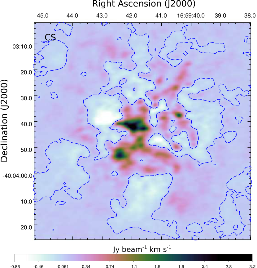
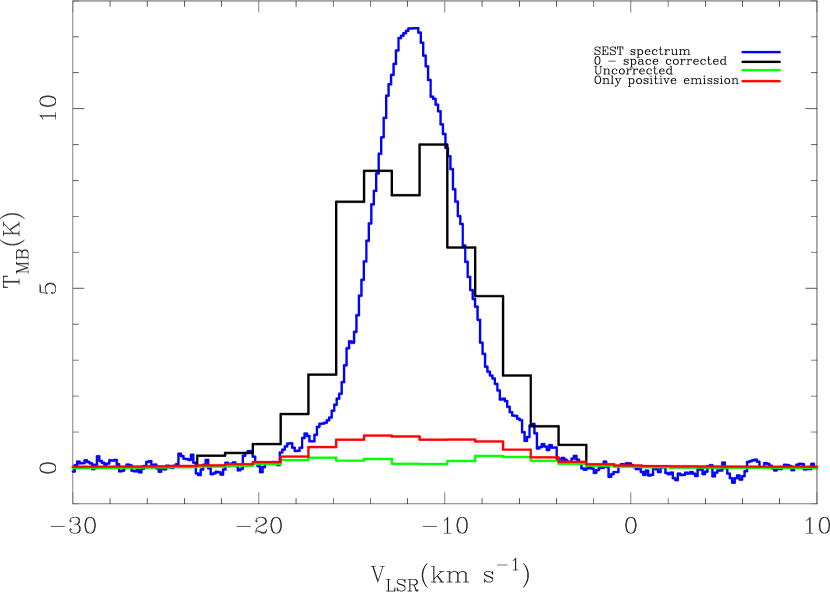
Figure A.1: Left panel: zero moment of the CS map. Dashed contours indicate the $-0.03$ Jy beam^-1 km s^-1 level. Right panel: in blue, we show the SEST CS, $J=2\shortrightarrow 1$ spectrum of IRAS 16562$-$3959 (Bronfman et al., 1996). Black and green lines show, respectively, the zero-space corrected and uncorrected CS spectra from the ALMA data cubes weighted by the SEST beam. The spectrum in red considers only the positive part of the emission from the ALMA cubes.

Appendix B Uncertainties of the Propyne Column density and temperature fitting

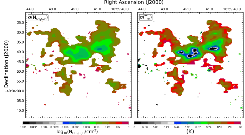
Figure B.1: Left and right panels show the formal uncertainties in the  column density and excitation temperature fitting, respectively (Section 4.2). The best-fit parameters are shown in Figure 12.

Appendix C Spectra From Conspicuous Sources

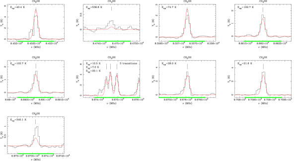
(a)

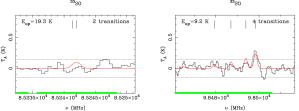
(b)

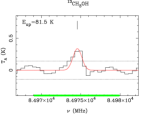
(c)

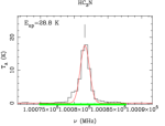
(d)

Figure C.1: Emission lines from several molecules toward the CC core, in K (primary beam corrected antenna temperatures) vs. frequency (MHz). Black and red continuous lines show the data and the model whose parameters are given in Table 5. In each panel we mark the $V_{\rm LSR}$ of the model with a vertical black line, and the upper energy level of each transition. Thick green lines indicate the section of the spectra used to get the best-fit values. In panels where the peak intensity does not reach $5\sigma$, $\sigma=0.06$ K we show the $\pm 2.5\sigma$ levels using dotted black lines. Panels (a) to (d) show CH₃OH, ³³SO, ¹³CH₃OH, and HC₃N, respectively.

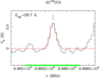
(e)

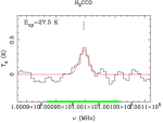
(f)

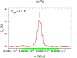
(g)

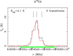
(h)

Figure C.1: (cont.) Same as the previous plot. Panels (e) to (h) show HC¹³CCN, H₂CCO, HC¹⁵N, and H¹³CN, respectively.

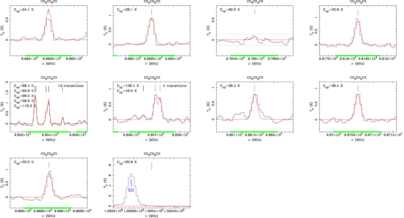
(i)

Figure C.1: (cont.) Same as the previous plot. Panels (i) show the C₂H₅CN lines.

(j)

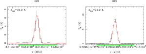
(k)

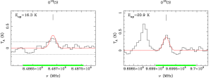
(l)

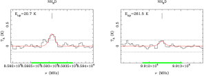
(m)

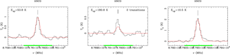
(n)

Figure C.1: (cont.) Same as the previous plot. Panels (j) to (n) show, respectively, CH₃CCH, OCS, O¹³CS, NH₂D, and HNCO.

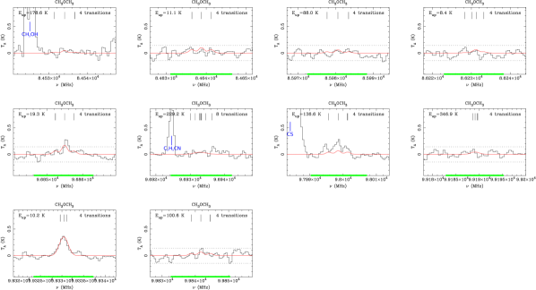
(o)

Figure C.1: (cont.) Same as the previous plot. Panel (o) shows the CH₃OCH₃ spectra of the CC core.

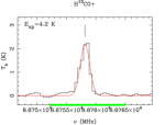
(p)

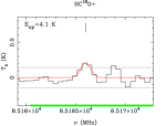
(q)

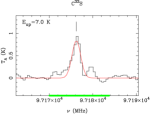
(r)

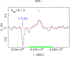
(s)

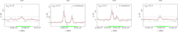
(t)

Figure C.1: (cont.) Same as the previous plot. Panels (q) to (r) show, respectively, the H¹³CO⁺, HC¹⁸O⁺, C³³S, HCS⁺, and CCH spectra of the CC core.

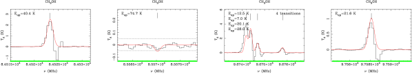
(a)

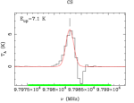
(b)

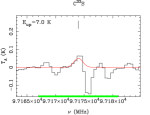
(c)

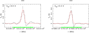
(d)

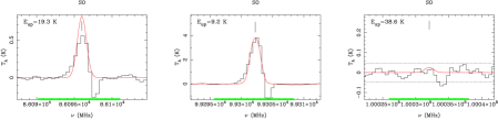
(e)

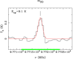
(f)

Figure C.2: Emission lines from several molecules toward the N-red cloud. Line types and colors as described in Figure C.1, with $\sigma=0.02$ K. Panels (a) to (f) show lines of CH₃OH, CS, C³³S, OCS, SO, and ³⁴SO, respectively.

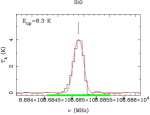
(g)

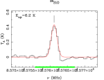
(h)

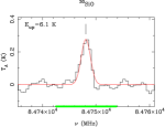
(i)

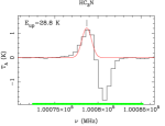
(j)

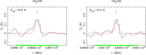
(k)

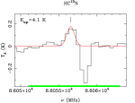
(l)

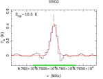
(m)

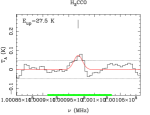
(n)

Figure C.2: (cont.) Same as in Figure C.2. Panels (g) to (n) show lines of SiO, ²⁹SiO, ³⁰SiO, HC₃N, CH₃CHO, HC¹⁵N, HNCO, and H₂CCO, respectively.

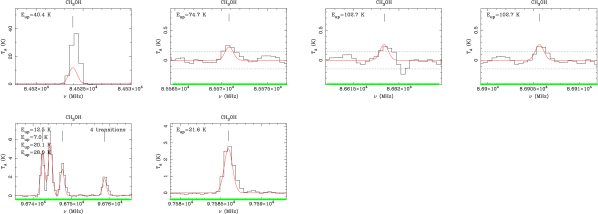
(a)

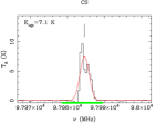
(b)

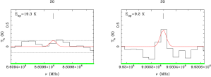
(c)

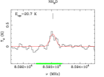
(d)

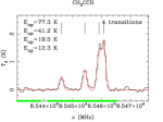
(e)

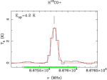
(f)

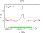
(g)

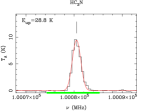
(h)

Figure C.3: Emission lines from several molecules toward the methanol peak of the NEC-wall. Line types and colors as described in Figure C.1, with $\sigma=0.06$ K. Panels (a) to (h) show lines of CH₃OH, CS, SO, NH₂D, CH₃CCH, H¹³CO⁺, HC¹⁸O⁺, and HC₃N, respectively.

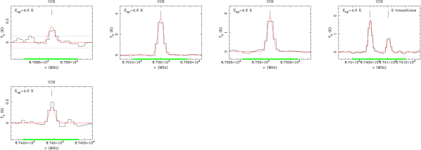
(i)

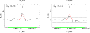
(j)

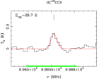
(k)

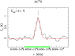
(l)

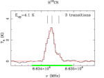
(m)

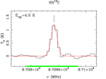
(n)

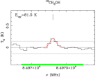
(o)

Figure C.3: (cont.) Same as Figure C.3. Panels (i) to (o) show lines of CCH, CH₃CHO, HC¹³CCN, HC¹⁵N, H¹³CN, and ¹³CH₃OH, respectively.

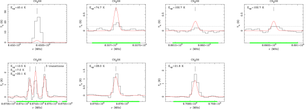
(a)

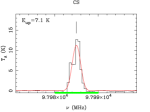
(b)

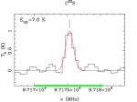
(c)

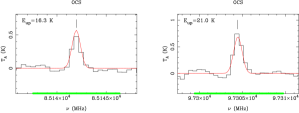
(d)

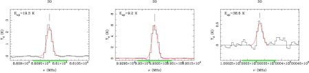
(e)

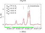
(f)

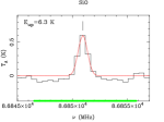
(g)

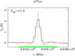
(h)

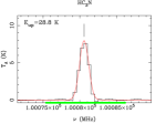
(i)

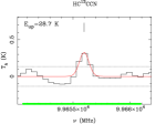
(j)

Figure C.4: Emission lines from several molecules toward the sulfur monoxide peak of the NEC-wall. Line types and colors as described in Figure C.1 with $\sigma=0.05$ K. Panels (a) to (j) show lines of CH₃OH, CS, C³³S, OCS, SO, CH₃CCH, SiO, H¹³CO⁺, HC₃N, and HC¹³CCN, respectively.

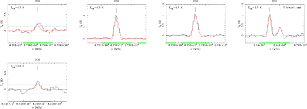
(k)

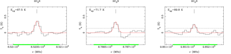
(l)

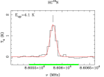
(m)

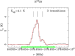
(n)

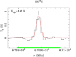
(o)

Figure C.4: (cont.) Same as Figure C.4. Panels (k) to (n) show lines of CCH, HC₅N, HC¹⁵N, H¹³CN, and HN¹³C, respectively.

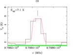
(a)

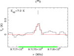
(b)

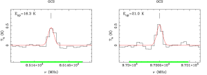
(c)

Figure C.5: Emission lines from several molecules toward the point (a) in the Diffuse ridge (DR (a)). Line types and colors as described in Figure C.1 with $\sigma=0.06$ K. Panels (a) to (c) show lines of CS, C³³S, and OCS, respectively.

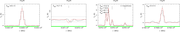
(d)

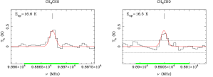
(e)

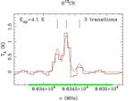
(f)

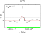
(g)

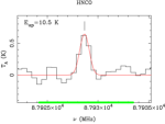
(h)

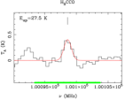
(i)

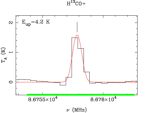
(j)

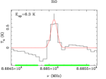
(k)

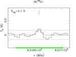
(l)

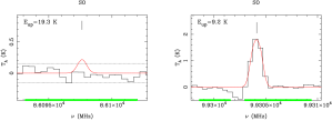
(m)

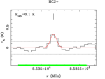
(n)

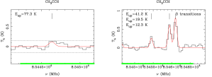
(o)

Figure C.5: (cont.) Same as Figure C.5. Panels (d) to (o) show lines of CH₃OH, CH₃CHO, H¹³CN, HC¹⁵N, HNCO, H₂CCO, H¹³CO⁺, SiO, HC¹⁸O⁺, SO, HCS⁺, and CH₃CCH, respectively.

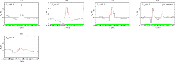
(p)

Figure C.5: (cont.) Same as Figure C.5. Panel (p) shows the CCH lines toward DR (a).

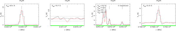
(a)

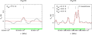
(b)

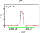
(c)

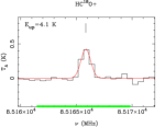
(d)

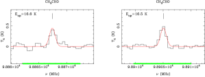
(e)

(f)

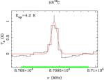
(g)

Figure C.6: Emission lines from several molecules toward the point (b) in the Diffuse ridge (DR (b)). Line types and colors as described in Figure C.1 with $\sigma=0.06$ K. Panels (a) to (g) show lines of CH₃OH, CH₃CCH, H¹³CO⁺, HC¹⁸O⁺, CH₃CHO, HC₃N, and HN¹³C, respectively.

(h)

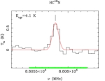
(i)

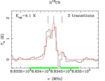
(j)

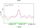
(k)

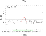
(l)

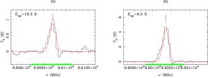
(m)

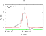
(n)

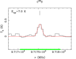
(o)

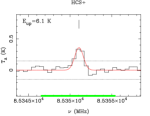
(p)

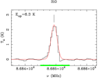
(q)

Figure C.6: (cont.) Same as Figure C.6. Panels (h) to (q) show lines of CCH, HC¹⁵N, H¹³CN, HNCO, ³⁴SO, SO, CS, C³³S, HCS⁺, and SiO, respectively.

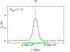
(a)

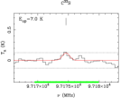
(b)

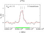
(c)

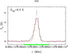
(d)

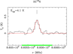
(e)

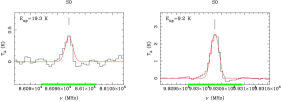
(f)

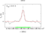
(g)

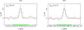
(h)

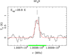
(i)

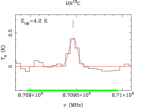
(j)

(k)

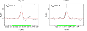
(l)

Figure C.7: Emission lines from several molecules toward the point (c) in the Diffuse ridge (DR (c)). Line types and colors as described in Figure C.1 with $\sigma=0.05$ K. Panels (a) to (l) show lines of CS, C³³S, H¹³CN, SiO, HC¹⁵N, SO, HNCO, OCS, HC₃N, HN¹³C, CH₃OH, and CH₃CHO, respectively.

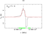
(a)

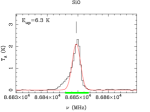
(b)

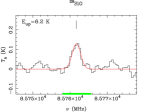
(c)

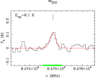
(d)

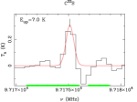
(e)

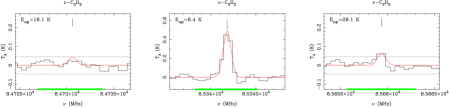
(f)

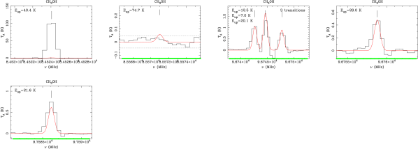
(g)

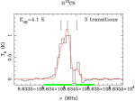
(h)

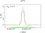
(i)

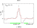
(j)

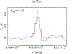
(k)

Figure C.8: Emission lines from several molecules toward the point S8E maser. Line types and colors as described in Figure C.1 with $\sigma=0.02$ K. Panels (a) to (k) show lines of CS, SiO, ²⁹SiO, ³⁰SiO, C³³S, c-C₃H₂, CH₃OH, H¹³CN, HN¹³C, HCS⁺, and HC¹⁸O⁺, respectively.

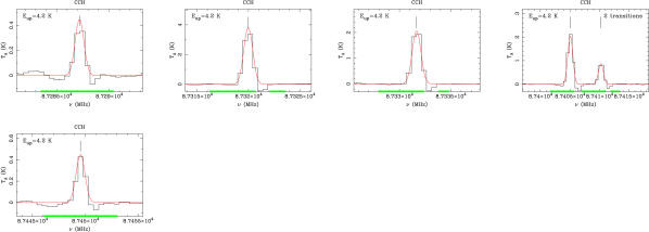
(l)

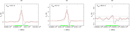
(m)

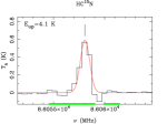
(n)

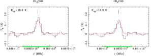
(o)

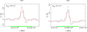
(p)

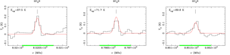
(q)

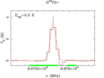
(r)

Figure C.8: (cont.) Same as Figure C.8. Panels (l) to (r) show lines of CCH, SO, HC¹⁵N, CH₃OH, OCS, HC₅N, and H¹³CO⁺, respectively.

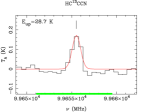
(s)

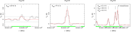
(t)

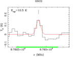
(u)

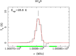
(v)

Figure C.8: (cont.) Same as Figure C.8. Panels (s) to (v) show lines of HC¹³CCN, CH₃CCH, HNCO, and HC₃N, respectively.

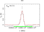
(a)

(b)

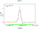
(c)

Figure C.9: Emission lines from several molecules toward the point S8E 1$\farcs$5 radius. Line types and colors as described in Figure C.1 with $\sigma=0.02$ K. Panels (a) to (c) show lines of SiO, SO, and HN¹³C, respectively.

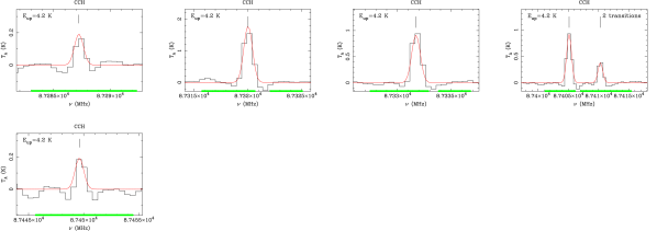
(d)

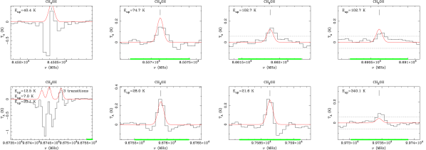
(e)

Figure C.9: (cont.) Same as Figure C.9. Panels (d) and (e) show the CCH and CH₃OH lines, respectively.

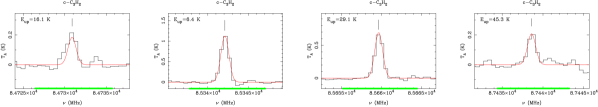
(f)

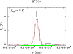
(g)

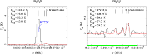
(h)

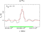
(i)

Figure C.9: (cont.) Same as Figure C.9. Panels (f) and (i) show the lines of c-C₃H₂, H¹³CO⁺, CH₃C₃N, and HC¹⁸O⁺, respectively.

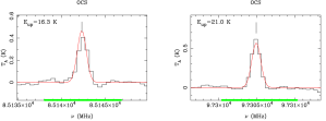
(j)

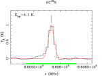
(k)

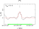
(l)

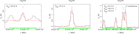
(m)

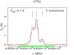
(n)

Figure C.9: (cont.) Same as Figure C.9. Panels (j) to (n) show the OCS, HC¹⁵N, C³³S, CH₃CCH, and H¹³CN  lines, respectively.

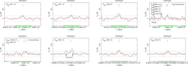
(o)

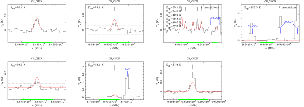
(p)

Figure C.9: (cont.) Same as Figure C.9. Panels (o) and (p) show the C₂H₅CN and CH₂CHCN lines, respectively. Panel (o) shows also the location of two possible lines of CH₃OCHO.

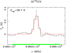
(q)

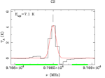
(r)

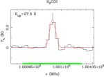
(s)

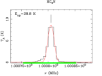
(t)

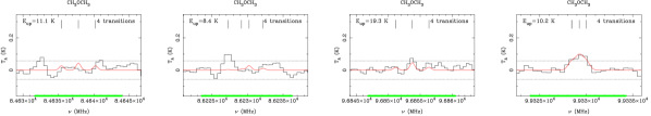
(u)

Figure C.9: (cont.) Same as Figure C.9. Panels (q) to (u) show the lines of HC¹³CCN, CS, H₂CCO, HC₃N, and CH₃OCH₃, respectively.

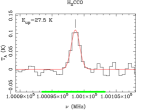
(a)

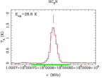
(b)

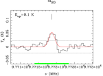
(c)

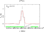
(d)

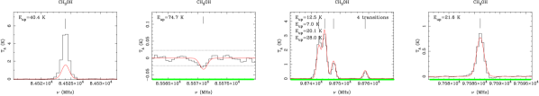
(e)

Figure C.10: Emission lines from several molecules toward the integrated NW cloud. Line types and colors as described in Figure C.1 with $\sigma=0.009$ K. Panels (a) to (e) show lines of H₂CCO, HC₃N, ³⁴SO, H¹³CO⁺, and CH₃OH, respectively.

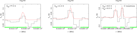
(f)

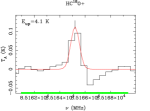
(g)

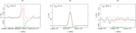
(h)

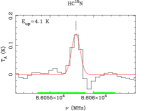
(i)

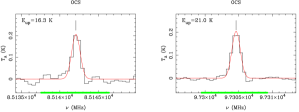
(j)

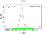
(k)

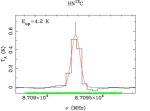
(l)

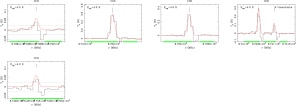
(m)

Figure C.10: (cont.) Same as Figure C.10. Panels (f) to (m) show lines of CH₃CCH, HC¹⁸O⁺, SO, HC¹⁵N, OCS, H¹³CN, HN¹³C, and CCH, respectively.

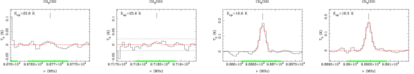
(n)

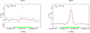
(o)

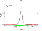
(p)

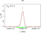
(q)

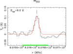
(r)

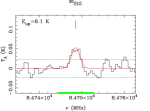
(s)

Figure C.10: (cont.) Same as Figure C.10. Panels (n) to (s) show lines of CH₃CHO, HNCO, CS, SiO, ²⁹SiO, and ³⁰SiO, respectively.

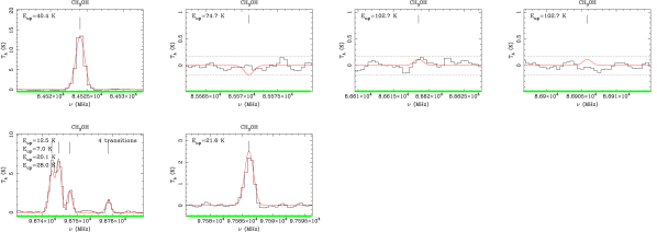
(a)

Figure C.11: CH₃OH lines from several molecules toward the point NW cloud (a), the methanol peak. Line types and colors as described in Figure C.1 with $\sigma=0.08$ K.

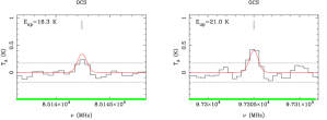
(b)

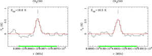
(c)

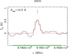
(d)

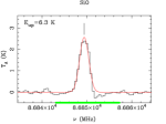
(e)

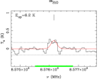
(f)

Figure C.11: (cont.) Same as Figure C.11. Panels (b) to (f) show lines of OCS, CH₃CHO, HNCO, SiO, and ²⁹SiO, respectively.

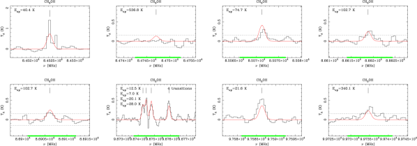
Figure C.12: Emission lines from CH₃OH toward Source 3. Line types and colors as described in Figure C.1 with $\sigma=0.05$ K.

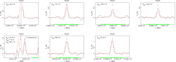
Figure C.13: Emission lines from CH₃OH toward Source 18. Line types and colors as described in Figure C.1 with $\sigma=0.05$ K.

References

- Adande & Ziurys (2012) Adande, G. R., & Ziurys, L. M. 2012, ApJ, 744, 194, doi: 10.1088/0004-637X/744/2/194
- Allen et al. (2017) Allen, V., van der Tak, F. F. S., Sánchez-Monge, Á., Cesaroni, R., & Beltrán, M. T. 2017, A&A, 603, A133, doi: 10.1051/0004-6361/201629118
- Asplund et al. (2009) Asplund, M., Grevesse, N., Sauval, A. J., & Scott, P. 2009, ARA&A, 47, 481, doi: 10.1146/annurev.astro.46.060407.145222
- Bally et al. (2017) Bally, J., Ginsburg, A., Arce, H., et al. 2017, ApJ, 837, 60, doi: 10.3847/1538-4357/aa5c8b
- Balucani et al. (2000) Balucani, N., Asvany, O., Huang, L. C. L., et al. 2000, ApJ, 545, 892, doi: 10.1086/317848
- Belloche et al. (2013) Belloche, A., Müller, H. S. P., Menten, K. M., Schilke, P., & Comito, C. 2013, A&A, 559, A47, doi: 10.1051/0004-6361/201321096
- Beltrán & de Wit (2016) Beltrán, M. T., & de Wit, W. J. 2016, A&A Rev., 24, 6, doi: 10.1007/s00159-015-0089-z
- Benjamin et al. (2003) Benjamin, R. A., Churchwell, E., Babler, B. L., et al. 2003, PASP, 115, 953, doi: 10.1086/376696
- Bergin et al. (1994) Bergin, E. A., Goldsmith, P. F., Snell, R. L., & Ungerechts, H. 1994, ApJ, 431, 674, doi: 10.1086/174518
- Bergin & Tafalla (2007) Bergin, E. A., & Tafalla, M. 2007, ARA&A, 45, 339, doi: 10.1146/annurev.astro.45.071206.100404
- Bergner et al. (2017) Bergner, J. B., Öberg, K. I., Garrod, R. T., & Graninger, D. M. 2017, ApJ, 841, 120, doi: 10.3847/1538-4357/aa72f6
- Beuther et al. (2009) Beuther, H., Zhang, Q., Bergin, E. A., & Sridharan, T. K. 2009, AJ, 137, 406, doi: 10.1088/0004-6256/137/1/406
- Beuther et al. (2006) Beuther, H., Zhang, Q., Sridharan, T. K., Lee, C.-F., & Zapata, L. A. 2006, A&A, 454, 221, doi: 10.1051/0004-6361:20064887
- Beuther et al. (2005) Beuther, H., Zhang, Q., Greenhill, L. J., et al. 2005, ApJ, 632, 355, doi: 10.1086/432974
- Bisschop et al. (2007) Bisschop, S. E., Jørgensen, J. K., van Dishoeck, E. F., & de Wachter, E. B. M. 2007, A&A, 465, 913, doi: 10.1051/0004-6361:20065963
- Blake et al. (1996) Blake, G. A., Mundy, L. G., Carlstrom, J. E., et al. 1996, ApJ, 472, L49, doi: 10.1086/310347
- Blake et al. (1987) Blake, G. A., Sutton, E. C., Masson, C. R., & Phillips, T. G. 1987, ApJ, 315, 621, doi: 10.1086/165165
- Bronfman et al. (1996) Bronfman, L., Nyman, L.-A., & May, J. 1996, A&AS, 115, 81
- Caselli et al. (1993) Caselli, P., Hasegawa, T. I., & Herbst, E. 1993, ApJ, 408, 548, doi: 10.1086/172612
- Caswell (1998) Caswell, J. L. 1998, MNRAS, 297, 215, doi: 10.1046/j.1365-8711.1998.01468.x
- Caswell (2009) —. 2009, PASA, 26, 454, doi: 10.1071/AS09013
- Caux et al. (2011) Caux, E., Bottinelli, S., Vastel, C., & Glorian, J. M. 2011, in IAU Symposium, Vol. 280, The Molecular Universe, ed. J. Cernicharo & R. Bachiller, 120
- Cesaroni et al. (2017) Cesaroni, R., Sánchez-Monge, Á., Beltrán, M. T., et al. 2017, A&A, 602, A59, doi: 10.1051/0004-6361/201630184
- Chapman et al. (2009) Chapman, J. F., Millar, T. J., Wardle, M., Burton, M. G., & Walsh, A. J. 2009, MNRAS, 394, 221, doi: 10.1111/j.1365-2966.2008.14144.x
- Charnley (1997) Charnley, S. B. 1997, ApJ, 481, 396, doi: 10.1086/304011
- Charnley (1999) Charnley, S. B. 1999, in NATO Advanced Science Institutes (ASI) Series C, Vol. 523, Formation and Evolution of Solids in Space, ed. J. M. Greenberg & A. Li (Springer Science+Business Media Dordrecht), 131
- Chin et al. (1996) Chin, Y.-N., Henkel, C., Whiteoak, J. B., Langer, N., & Churchwell, E. B. 1996, A&A, 305, 960
- Colzi et al. (2018) Colzi, L., Fontani, F., Rivilla, V. M., Sánchez-Monge, A., Testi, L., Beltrán, M. T., Caselli, P. 2018, MNRAS, doi: 10.1093/mnras/sty1027
- Cosentino et al. (2018) Cosentino, G., Jiménez-Serra, I., Henshaw, J. D., et al. 2018, MNRAS, 474, 3760, doi: 10.1093/mnras/stx3013
- Cragg et al. (1992) Cragg, D. M., Johns, K. P., Godfrey, P. D., & Brown, R. D. 1992, MNRAS, 259, 203, doi: 10.1093/mnras/259.1.203
- Crockett et al. (2015) Crockett, N. R., Bergin, E. A., Neill, J. L., et al. 2015, ApJ, 806, 239, doi: 10.1088/0004-637X/806/2/239
- Dahmen et al. (1995) Dahmen, G., Wilson, T. L., & Matteucci, F. 1995, A&A, 295, 194
- Dame (2011) Dame, T. M. 2011, ArXiv e-prints. https://arxiv.org/abs/1101.1499
- Danilovich et al. (2016) Danilovich, T., De Beck, E., Black, J. H., Olofsson, H., & Justtanont, K. 2016, A&A, 588, A119, doi: 10.1051/0004-6361/201527943
- Fayolle et al. (2015) Fayolle, E. C., Öberg, K. I., Garrod, R. T., van Dishoeck, E. F., & Bisschop, S. E. 2015, A&A, 576, A45, doi: 10.1051/0004-6361/201323114
- Fedoseev et al. (2015) Fedoseev, G., Ioppolo, S., & Linnartz, H. 2015, MNRAS, 446, 449, doi: 10.1093/mnras/stu1852
- Feng et al. (2015) Feng, S., Beuther, H., Henning, T., et al. 2015, A&A, 581, A71, doi: 10.1051/0004-6361/201322725
- Ferrante et al. (2008) Ferrante, R. F., Moore, M. H., Spiliotis, M. M., & Hudson, R. L. 2008, ApJ, 684, 1210, doi: 10.1086/590362
- Fontani et al. (2007) Fontani, F., Pascucci, I., Caselli, P., et al. 2007, A&A, 470, 639, doi: 10.1051/0004-6361:20077485
- Friberg et al. (1988) Friberg, P., Hjalmarson, A., Madden, S. C., & Irvine, W. M. 1988, A&A, 195, 281
- Friedel & Widicus Weaver (2012) Friedel, D. N., & Widicus Weaver, S. L. 2012, ApJS, 201, 17, doi: 10.1088/0067-0049/201/2/17
- Garrod et al. (2008) Garrod, R. T., Widicus Weaver, S. L., & Herbst, E. 2008, ApJ, 682, 283, doi: 10.1086/588035
- Giannetti et al. (2017) Giannetti, A., Leurini, S., Wyrowski, F., et al. 2017, A&A, 603, A33, doi: 10.1051/0004-6361/201630048
- Gibb et al. (2000) Gibb, E., Nummelin, A., Irvine, W. M., Whittet, D. C. B., & Bergman, P. 2000, ApJ, 545, 309, doi: 10.1086/317805
- Gibb et al. (2004) Gibb, E. L., Whittet, D. C. B., Boogert, A. C. A., & Tielens, A. G. G. M. 2004, ApJS, 151, 35, doi: 10.1086/381182
- Gong et al. (2015) Gong, Y., Henkel, C., Thorwirth, S., et al. 2015, A&A, 581, A48, doi: 10.1051/0004-6361/201526275
- Gottlieb et al. (1983) Gottlieb, C. A., Gottlieb, E. W., & Thaddeus, P. 1983, ApJ, 264, 740, doi: 10.1086/160647
- Graninger et al. (2014) Graninger, D. M., Herbst, E., Öberg, K. I., & Vasyunin, A. I. 2014, ApJ, 787, 74, doi: 10.1088/0004-637X/787/1/74
- Guzmán et al. (2010) Guzmán, A. E., Garay, G., & Brooks, K. J. 2010, ApJ, 725, 734, doi: 10.1088/0004-637X/725/1/734
- Guzmán et al. (2011) Guzmán, A. E., Garay, G., Brooks, K. J., Rathborne, J., & Güsten, R. 2011, ApJ, 736, 150, doi: 10.1088/0004-637X/736/2/150
- Guzmán et al. (2016) Guzmán, A. E., Garay, G., Rodríguez, L. F., et al. 2016, ApJ, 826, 208, doi: 10.3847/0004-637X/826/2/208
- Guzmán et al. (2018) Guzmán, A. E., Guzmán, V. V., Garay, G., Bronfman, L., & Hechenleitner, F. 2018, Replication data for: Chemistry of the High-Mass Protostellar Molecular Clump IRAS 165623959, 1.0, Harvard Dataverse, doi: 10.7910/DVN/VNXS9R.
- Guzmán et al. (2015a) Guzmán, A. E., Sanhueza, P., Contreras, Y., et al. 2015a, ApJ, 815, 130, doi: 10.1088/0004-637X/815/2/130
- Guzmán et al. (2014) Guzmán, A. E., Garay, G., Rodríguez, L. F., et al. 2014, ApJ, 796, 117
- Guzmán et al. (2017) Guzmán, V. V., Öberg, K. I., Huang, J., Loomis, R., & Qi, C. 2017, ApJ, 836, 30, doi: 10.3847/1538-4357/836/1/30
- Guzmán et al. (2015b) Guzmán, V. V., Öberg, K. I., Loomis, R., & Qi, C. 2015b, ApJ, 814, 53, doi: 10.1088/0004-637X/814/1/53
- Harju et al. (1998) Harju, J., Lehtinen, K., Booth, R. S., & Zinchenko, I. 1998, A&AS, 132, 211, doi: 10.1051/aas:1998448
- Heays et al. (2014) Heays, A. N., Visser, R., Gredel, R., et al. 2014, A&A, 562, A61, doi: 10.1051/0004-6361/201322832
- Heiderman et al. (2010) Heiderman, A., Evans, II, N. J., Allen, L. E., Huard, T., & Heyer, M. 2010, ApJ, 723, 1019, doi: 10.1088/0004-637X/723/2/1019
- Herbst (1978) Herbst, E. 1978, ApJ, 222, 508, doi: 10.1086/156163
- Herbst & Klemperer (1973) Herbst, E., & Klemperer, W. 1973, ApJ, 185, 505, doi: 10.1086/152436
- Herbst & Leung (1990) Herbst, E., & Leung, C. M. 1990, A&A, 233, 177
- Herbst & van Dishoeck (2009) Herbst, E., & van Dishoeck, E. F. 2009, ARA&A, 47, 427, doi: 10.1146/annurev-astro-082708-101654
- Hirota et al. (1998) Hirota, T., Yamamoto, S., Mikami, H., & Ohishi, M. 1998, ApJ, 503, 717, doi: 10.1086/306032
- Immer et al. (2014) Immer, K., Galván-Madrid, R., König, C., Liu, H. B., & Menten, K. M. 2014, A&A, 572, A63, doi: 10.1051/0004-6361/201423780
- Jiménez-Serra et al. (2008) Jiménez-Serra, I., Caselli, P., Martín-Pintado, J., & Hartquist, T. W. 2008, A&A, 482, 549, doi: 10.1051/0004-6361:20078054
- Jiménez-Serra et al. (2005) Jiménez-Serra, I., Martín-Pintado, J., Rodríguez-Franco, A., & Martín, S. 2005, ApJ, 627, L121, doi: 10.1086/432467
- Jiménez-Serra et al. (2012) Jiménez-Serra, I., Zhang, Q., Viti, S., Martín-Pintado, J., & de Wit, W.-J. 2012, ApJ, 753, 34, doi: 10.1088/0004-637X/753/1/34
- Jin et al. (2015) Jin, M., Lee, J.-E., & Kim, K.-T. 2015, ApJS, 219, 2, doi: 10.1088/0067-0049/219/1/2
- Kelly et al. (2017) Kelly, G., Viti, S., García-Burillo, S., et al. 2017, A&A, 597, A11, doi: 10.1051/0004-6361/201628946
- Lackington et al. (2016) Lackington, M., Fuller, G. A., Pineda, J. E., et al. 2016, MNRAS, 455, 806, doi: 10.1093/mnras/stv2354
- Lampton et al. (1976) Lampton, M., Margon, B., & Bowyer, S. 1976, ApJ, 208, 177, doi: 10.1086/154592
- Lefloch et al. (2017) Lefloch, B., Ceccarelli, C., Codella, C., et al. 2017, MNRAS, 469, L73, doi: 10.1093/mnrasl/slx050
- López-Calderón et al. (2016) López-Calderón, C., Bronfman, L., Nyman, L.-Å., et al. 2016, A&A, 595, A88, doi: 10.1051/0004-6361/201321696
- Lu et al. (2017) Lu, X., Zhang, Q., Kauffmann, J., et al. 2017, ApJ, 839, 1, doi: 10.3847/1538-4357/aa67f7
- Miettinen et al. (2006) Miettinen, O., Harju, J., Haikala, L. K., & Pomrén, C. 2006, A&A, 460, 721, doi: 10.1051/0004-6361:20064815
- Milam et al. (2005) Milam, S. N., Savage, C., Brewster, M. A., Ziurys, L. M., & Wyckoff, S. 2005, ApJ, 634, 1126, doi: 10.1086/497123
- Minniti et al. (2010) Minniti, D., Lucas, P. W., Emerson, J. P., et al. 2010, New A, 15, 433, doi: 10.1016/j.newast.2009.12.002
- Molinari et al. (2016) Molinari, S., Merello, M., Elia, D., et al. 2016, ApJ, 826, L8, doi: 10.3847/2041-8205/826/1/L8
- Monson et al. (2017) Monson, N. N., Morris, M. R., & Young, E. D. 2017, ApJ, 839, 123, doi: 10.3847/1538-4357/aa67e6
- Mookerjea et al. (2007) Mookerjea, B., Casper, E., Mundy, L. G., & Looney, L. W. 2007, ApJ, 659, 447, doi: 10.1086/512095
- Müller et al. (2005) Müller, H. S. P., Schlöder, F., Stutzki, J., & Winnewisser, G. 2005, Journal of Molecular Structure, 742, 215, doi: 10.1016/j.molstruc.2005.01.027
- Öberg et al. (2013) Öberg, K. I., Boamah, M. D., Fayolle, E. C., et al. 2013, ApJ, 771, 95, doi: 10.1088/0004-637X/771/2/95
- Öberg et al. (2014) Öberg, K. I., Fayolle, E. C., Reiter, J. B., & Cyganowski, C. 2014, Faraday Discussions, 168, 81, doi: 10.1039/C3FD00146F
- Olofsson (2005) Olofsson, H. 2005, in IAU Symposium, Vol. 231, Astrochemistry: Recent Successes and Current Challenges, ed. D. C. Lis, G. A. Blake, & E. Herbst, 499–508
- Palau et al. (2017) Palau, A., Walsh, C., Sánchez-Monge, Á., et al. 2017, MNRAS, 467, 2723, doi: 10.1093/mnras/stx004
- Penzias (1981) Penzias, A. A. 1981, ApJ, 249, 513, doi: 10.1086/159310
- Persson et al. (2007) Persson, C. M., Olofsson, A. O. H., Koning, N., et al. 2007, A&A, 476, 807, doi: 10.1051/0004-6361:20077225
- Petry & CASA Development Team (2012) Petry, D., & CASA Development Team. 2012, in Astronomical Society of the Pacific Conference Series, Vol. 461, Astronomical Data Analysis Software and Systems XXI, ed. P. Ballester, D. Egret, & N. P. F. Lorente, 849
- Pickett et al. (1998) Pickett, H. M., Poynter, R. L., Cohen, E. A., et al. 1998, J. Quant. Spec. Radiat. Transf., 60, 883, doi: 10.1016/S0022-4073(98)00091-0
- Pineau des Forets et al. (1993) Pineau des Forets, G., Roueff, E., Schilke, P., & Flower, D. R. 1993, MNRAS, 262, 915, doi: 10.1093/mnras/262.4.915
- Plunkett et al. (2013) Plunkett, A. L., Arce, H. G., Corder, S. A., et al. 2013, ApJ, 774, 22, doi: 10.1088/0004-637X/774/1/22
- Podio et al. (2015) Podio, L., Codella, C., Gueth, F., et al. 2015, A&A, 581, A85, doi: 10.1051/0004-6361/201525778
- Prasad & Huntress (1980) Prasad, S. S., & Huntress, Jr., W. T. 1980, ApJS, 43, 1, doi: 10.1086/190665
- Qin et al. (2010) Qin, S.-L., Wu, Y., Huang, M., et al. 2010, ApJ, 711, 399, doi: 10.1088/0004-637X/711/1/399
- Rathborne et al. (2006) Rathborne, J. M., Jackson, J. M., & Simon, R. 2006, ApJ, 641, 389, doi: 10.1086/500423
- Rieke & Lebofsky (1985) Rieke, G. H., & Lebofsky, M. J. 1985, ApJ, 288, 618, doi: 10.1086/162827
- Rodríguez-Fernández et al. (2010) Rodríguez-Fernández, N. J., Tafalla, M., Gueth, F., & Bachiller, R. 2010, A&A, 516, A98, doi: 10.1051/0004-6361/201013997
- Roueff et al. (2005) Roueff, E., Lis, D. C., van der Tak, F. F. S., Gerin, M., & Goldsmith, P. F. 2005, A&A, 438, 585, doi: 10.1051/0004-6361:20052724
- Sakai & Yamamoto (2013) Sakai, N., & Yamamoto, S. 2013, Chemical Reviews, 113, 8981, doi: 10.1021/cr4001308
- Sakai et al. (2013) Sakai, T., Sakai, N., Foster, J. B., et al. 2013, ApJ, 775, L31, doi: 10.1088/2041-8205/775/1/L31
- Sanhueza et al. (2013) Sanhueza, P., Jackson, J. M., Foster, J. B., et al. 2013, ApJ, 773, 123, doi: 10.1088/0004-637X/773/2/123
- Schiff & Bohme (1979) Schiff, H. I., & Bohme, D. K. 1979, ApJ, 232, 740, doi: 10.1086/157334
- Schilke et al. (1992) Schilke, P., Walmsley, C. M., Pineau Des Forets, G., et al. 1992, A&A, 256, 595
- Schöier et al. (2005) Schöier, F. L., van der Tak, F. F. S., van Dishoeck, E. F., & Black, J. H. 2005, A&A, 432, 369, doi: 10.1051/0004-6361:20041729
- Shirley (2015) Shirley, Y. L. 2015, PASP, 127, 299, doi: 10.1086/680342
- Su et al. (2005) Su, Y.-N., Liu, S.-Y., Lim, J., & Chen, H.-R. 2005, in Protostars and Planets V Posters, Vol. 1286, 8336
- Suutarinen et al. (2014) Suutarinen, A. N., Kristensen, L. E., Mottram, J. C., Fraser, H. J., & van Dishoeck, E. F. 2014, MNRAS, 440, 1844, doi: 10.1093/mnras/stu406
- Tan et al. (2014) Tan, J. C., Beltrán, M. T., Caselli, P., et al. 2014, Protostars and Planets VI, 149, doi: 10.2458/azu_uapress_9780816531240-ch007
- Tercero et al. (2010) Tercero, B., Cernicharo, J., Pardo, J. R., & Goicoechea, J. R. 2010, A&A, 517, A96, doi: 10.1051/0004-6361/200913501
- Tielens (2013) Tielens, A. G. G. M. 2013, Reviews of Modern Physics, 85, 1021, doi: 10.1103/RevModPhys.85.1021
- Townes & Schawlow (1975) Townes, C. H., & Schawlow, A. L. 1975, Microwave spectroscopy. (Dover Publications Inc., Mineola, New York)
- Ueda et al. (2017) Ueda, J., Watanabe, Y., Iono, D., et al. 2017, PASJ, 69, 6, doi: 10.1093/pasj/psw110
- Urquhart et al. (2007) Urquhart, J. S., Busfield, A. L., Hoare, M. G., et al. 2007, A&A, 474, 891, doi: 10.1051/0004-6361:20078025
- van der Tak (2011) van der Tak, F. 2011, in IAU Symposium, Vol. 280, IAU Symposium, ed. J. Cernicharo & R. Bachiller, 449–460
- van der Tak et al. (2007) van der Tak, F. F. S., Black, J. H., Schöier, F. L., Jansen, D. J., & van Dishoeck, E. F. 2007, A&A, 468, 627, doi: 10.1051/0004-6361:20066820
- van Dishoeck & Blake (1998) van Dishoeck, E. F., & Blake, G. A. 1998, ARA&A, 36, 317, doi: 10.1146/annurev.astro.36.1.317
- Vastel et al. (2014) Vastel, C., Ceccarelli, C., Lefloch, B., & Bachiller, R. 2014, ApJ, 795, L2, doi: 10.1088/2041-8205/795/1/L2
- Vasyunina et al. (2014) Vasyunina, T., Vasyunin, A. I., Herbst, E., et al. 2014, ApJ, 780, 85, doi: 10.1088/0004-637X/780/1/85
- Viti et al. (2004) Viti, S., Collings, M. P., Dever, J. W., McCoustra, M. R. S., & Williams, D. A. 2004, MNRAS, 354, 1141, doi: 10.1111/j.1365-2966.2004.08273.x
- Voronkov et al. (2006) Voronkov, M. A., Brooks, K. J., Sobolev, A. M., et al. 2006, MNRAS, 373, 411, doi: 10.1111/j.1365-2966.2006.11047.x
- Wampfler et al. (2014) Wampfler, S. F., Jørgensen, J. K., Bizzarro, M., & Bisschop, S. E. 2014, A&A, 572, A24, doi: 10.1051/0004-6361/201423773
- Wang et al. (2011) Wang, Y., Beuther, H., Bik, A., et al. 2011, A&A, 527, A32, doi: 10.1051/0004-6361/201015543
- Wannier et al. (1981) Wannier, P. G., Linke, R. A., & Penzias, A. A. 1981, ApJ, 247, 522, doi: 10.1086/159062
- Watanabe et al. (2016) Watanabe, Y., Sakai, N., Sorai, K., Ueda, J., & Yamamoto, S. 2016, ApJ, 819, 144, doi: 10.3847/0004-637X/819/2/144
- Widicus Weaver & Friedel (2012) Widicus Weaver, S. L., & Friedel, D. N. 2012, ApJS, 201, 16, doi: 10.1088/0067-0049/201/2/16
- Wienen et al. (2012) Wienen, M., Wyrowski, F., Schuller, F., et al. 2012, A&A, 544, A146, doi: 10.1051/0004-6361/201118107
- Wilson (1999) Wilson, T. L. 1999, Reports on Progress in Physics, 62, 143, doi: 10.1088/0034-4885/62/2/002
- Wilson & Rood (1994) Wilson, T. L., & Rood, R. 1994, ARA&A, 32, 191, doi: 10.1146/annurev.aa.32.090194.001203
- Wootten & Thompson (2009) Wootten, A., & Thompson, A. R. 2009, IEEE Proceedings, 97, 1463, doi: 10.1109/JPROC.2009.2020572
- Wright et al. (1996) Wright, M. C. H., Plambeck, R. L., & Wilner, D. J. 1996, ApJ, 469, 216, doi: 10.1086/177773
- Yamamoto (2017) Yamamoto, S. 2017, Introduction to Astrochemistry: Chemical Evolution from Interstellar Clouds to Star and Planet Formation (Springer), doi: 10.1007/978-4-431-54171-4
- Zapata et al. (2013) Zapata, L. A., Schmid-Burgk, J., Pérez-Goytia, N., et al. 2013, ApJ, 765, L29, doi: 10.1088/2041-8205/765/2/L29