Improving information centrality of a node in complex networks by adding edges

Abstract

The problem of increasing the centrality of a network node arises in many practical applications. In this paper, we study the optimization problem of maximizing the information centrality $I_{v}$ of a given node $v$ in a network with $n$ nodes and $m$ edges, by creating $k$ new edges incident to $v$. Since $I_{v}$ is the reciprocal of the sum of resistance distance $\mathcal{R}_{v}$ between $v$ and all nodes, we alternatively consider the problem of minimizing $\mathcal{R}_{v}$ by adding $k$ new edges linked to $v$. We show that the objective function is monotone and supermodular. We provide a simple greedy algorithm with an approximation factor $\left(1-\frac{1}{e}\right)$ and $O(n^{3})$ running time. To speed up the computation, we also present an algorithm to compute $\left(1-\frac{1}{e}-\epsilon\right)$-approximate resistance distance $\mathcal{R}_{v}$ after iteratively adding $k$ edges, the running time of which is $\mathaccent 869{O}(mk\epsilon^{-2})$ for any $\epsilon>0$, where the $\mathaccent 869{O}(\cdot)$ notation suppresses the ${\rm poly}(\log n)$ factors. We experimentally demonstrate the effectiveness and efficiency of our proposed algorithms.

1 Introduction

Centrality metrics refer to indicators identifying the varying importance of nodes in complex networks Lü et al. (2016), which have become a powerful tool in network analysis and found wide applications in network science Newman (2010). Over the past years, a great number of centrality indices and corresponding algorithms have been proposed to analyze and understand the roles of nodes in networks White and Smyth (2003); Boldi and Vigna (2014). Among various centrality indices, betweennees centrality and closeness centrality are probably the two most frequently used ones, especially in social network analysis. However, both indicators only consider the shortest paths, excluding the contributions from other longer paths. In order to overcome the drawback of these two measures, current flow closeness centrality Brandes and Fleischer (2005); Newman (2005) was introduced and proved to be exactly the information centrality Stephenson and Zelen (1989), which counts all possible paths between nodes and has a better discriminating power than betweennees centrality Newman (2005) and closeness centrality Bergamini et al. (2016).

It is recognized that centrality measures have proved of great significance in complex networks. Having high centrality can have positive consequences on the node itself. In this paper, we consider the problem of adding a given number of edges incident to a designated node $v$ so as to maximize the centrality of $v$. Our main motivation or justification for studying this problem is that it has several application scenarios, including airport networks Ishakian et al. (2012), recommendation systems Parotsidis et al. (2016), among others. For example, in airport networks, a node (airport) has the incentive to improve as much as possible its centrality (transportation capacity) by adding edges (directing flights) connecting itself and other nodes (airports) Ishakian et al. (2012). Another example is the link recommendation problem of recommending to a user $v$ a given number of links from a set of candidate inexistent links incident to $v$ in order to minimize the shortest distance from $v$ to other nodes Parotsidis et al. (2016).

The problem of maximizing the centrality of a specific target node through adding edges incident to it has been widely studied. For examples, some authors have studied the problem of creating $k$ edges linked to a node $v$ so that the centrality value for $v$ with respect to concerned centrality measures is maximized, e.g., betweenness centrality Crescenzi et al. (2015); D’Angelo et al. (2016); Crescenzi et al. (2016); Hoffmann et al. (2018) and closeness centrality Crescenzi et al. (2015); Hoffmann et al. (2018). Similar optimization problems for a predefined node $v$ were also addressed for other node centrality metrics, including average shortest distance between $v$ and remaining nodes Meyerson and Tagiku (2009); Parotsidis et al. (2016), largest distance from $v$ to other nodes Demaine and Zadimoghaddam (2010), PageRank Avrachenkov and Litvak (2006); Olsen (2010), and the number of different paths containing $v$ Ishakian et al. (2012). However, previous works do not consider improving information centrality of a node by adding new edges linked to it, despite the fact that it can better distinguish different nodes, compared with betweennees  Newman (2005) and closeness centrality Bergamini et al. (2016).

In this paper, we study the following problem: Given a graph with $n$ nodes and $m$ edges, how to create $k$ new edges incident to a designated node $v$, so that the information centrality $I_{v}$ of $v$ is maximized. Since $I_{v}$ equals the reciprocal of the sum of resistance distance $\mathcal{R}_{v}$ between $v$ and all nodes, we reduce the problem to minimizing $\mathcal{R}_{v}$ by introducing $k$ edges connecting $v$. We demonstrate that the optimization function is monotone and supermodular. To minimize resistance distance $\mathcal{R}_{v}$, we present two greedy approximation algorithms by iteratively introducing $k$ edges one by one. The former is a $\left(1-\frac{1}{e}\right)$-approximation algorithm with $O(n^{3})$ time complexity, while the latter is a $\left(1-\frac{1}{e}-\epsilon\right)$-approximation algorithm with $\mathaccent 869{O}(mk\epsilon^{-2})$ time complexity, where the $\mathaccent 869{O}(\cdot)$ notation hides ${\rm poly}(\log n)$ factors. We test the performance of our algorithms on several model and real networks, which substantially increase information centrality score of a given node and outperform several other adding edge strategies.

2 Preliminary

Consider a connected undirected weighted network $G=(V,E,w)$ where $V$ is the set of nodes, $E\subseteq V\times V$ is the set of edges, and $w:E\to\mathbb{R}_{+}$ is the edge weight function. We use $w_{max}$ to denote the maximum edge weight. Let $n=|V|$ denote the number of nodes and $m=|E|$ denote the number of edges. For a pair of adjacent nodes $u$ and $v$, we write $u\sim v$ to denote $(u,v)\in E$. The Laplacian matrix of $G$ is the symmetric matrix $\bm{\mathit{L}}=\bm{\mathit{D}}-\bm{\mathit{A}}$, where $\bm{\mathit{A}}$ is the weighted adjacency matrix of the graph and $\bm{\mathit{D}}$ is the degree diagonal matrix.

Let $\bm{\mathit{e}}_{i}$ denote the $i$th standard basis vector, and $\bm{\mathit{b}}_{u,v}=\bm{\mathit{e}}_{u}-\bm{\mathit{e}}_{v}$. We fix an arbitrary orientation for all edges in $G$. For each edge $e\in E$, we define $\bm{\mathit{b}}_{e}=\bm{\mathit{b}}_{u,v}$, where $u$ and $v$ are head and tail of $e$, respectively. It is easy to verify that $\bm{\mathit{L}}=\sum\nolimits_{e\in E}w(e)\bm{\mathit{b}}_{e}\bm{\mathit{b}}_{e}^{\top}$, where $w(e)\bm{\mathit{b}}_{e}\bm{\mathit{b}}_{e}^{\top}$ is the Laplacian of $e$. $\bm{\mathit{L}}$ is singular and positive semidefinite. Its pseudoinverse $\bm{\mathit{L}}^{\dagger}$ is $\left(\bm{\mathit{L}}+\frac{1}{n}\bm{\mathit{J}}\right)^{-1}-\frac{1}{n}\bm{\mathit{J}}$, where $\bm{\mathit{J}}$ is the matrix with all entries being ones.

For network $G=(V,E,w)$, the resistance distance Klein and Randić (1993) between two nodes $u,v$ is $\mathcal{R}_{uv}=\bm{\mathit{b}}_{u,v}^{\top}\bm{\mathit{L}}^{\dagger}\bm{\mathit{b}}_{u,v}$. The resistance distance $\mathcal{R}_{v}$ of a node $v$ is the sum of resistance distances between $v$ and all nodes in $V$, that is, $\mathcal{R}_{v}=\sum_{u\in V}\mathcal{R}_{uv}$, which can be expressed in terms of the entries of $\bm{\mathit{L}}^{\dagger}$ as Bozzo and Franceschet (2013)

$$\mathcal{R}_{v}=n\bm{\mathit{L}}^{\dagger}_{vv}+\mathrm{Tr}\left(\bm{\mathit{L}}^{\dagger}\right).$$ (1)

Let $\bm{\mathit{L}}_{v}$ denote the submatrix of Laplacian $\bm{\mathit{L}}$, which is obtained from $\bm{\mathit{L}}$ by deleting the row and column corresponding to node $v$. For a connected graph $G$, $\bm{\mathit{L}}_{v}$ is invertible for any node $v$, and the resistance distance $\mathcal{R}_{uv}$ between $v$ and another node $u$ is equal to $\left(\bm{\mathit{L}}_{v}^{-1}\right)_{uu}$ Izmailian et al. (2013). Thus, we have

$$\mathcal{R}_{v}=\mathrm{Tr}\left(\bm{\mathit{L}}_{v}^{-1}\right).$$ (2)

The resistance distance $\mathcal{R}_{v}$ can be used as a measure of the efficiency for node $v$ in transmitting information to other nodes, and is closely related to information centrality introduced by Stephenson and Zelen to measure the importance of nodes in social networks Stephenson and Zelen (1989). The information $I_{uv}$ transmitted between $u$ and $v$ is defined as

$$I_{uv}=\frac{1}{\bm{\mathit{B}}^{-1}(u,u)+\bm{\mathit{B}}^{-1}(v,v)-2\bm{\mathit{B}}^{-1}(u,v)},$$

where $\bm{\mathit{B}}=\bm{\mathit{L}}+\bm{\mathit{J}}$. The information centrality $I_{v}$ of node $v$ is the harmonic mean of $I_{uv}$ over all nodes $u$ Stephenson and Zelen (1989).

Definition 2.1

For a connected graph $G=(V,E,w)$, the information centrality $I_{v}$ of a node $v\in V$ is defined as

$$I_{v}=\frac{n}{\sum\limits_{u\in V}1/I_{uv}}.$$

It was shown Brandes and Fleischer (2005) that

$$I_{v}=\frac{n}{\mathcal{R}_{v}}.$$ (3)

We continue to introduce some useful notations and tools for the convenience of description for our algorithms, including $\epsilon$-approximation and supermodular function.

Let $a,b\geq 0$ be two nonnegative scalars. We say $a$ is an $\epsilon$-approximation Peng and Spielman (2014) of $b$ if $\exp(-\epsilon)\,a\leq b\leq\exp(\epsilon)\,a$. Hereafter, we use $a\approx_{\epsilon}b$ to represent that $a$ is an $\epsilon$-approximation of $b$.

Let $X$ be a finite set, and $2^{X}$ be the set of all subsets of $X$. Let $f:2^{X}\to\mathbb{R}$ be a set function on $X$. For any subsets $S\subset T\subset X$ and any element $a\in X\setminus T$, we say function $f(\cdot)$ is supermodular if it satisfies $f(S)-f(S\cup\{a\})\geq f(T)-f(T\cup\{a\})$. A function $f(\cdot)$ is submodular if $-f(\cdot)$ is supermodular. A set function $f:2^{X}\to\mathbb{R}$ is called monotone decreasing if for any subsets $S\subset T\subset X$, $f(S)>f(T)$ holds.

3 Problem Formulation

For a connected undirected weighted network $G(V,E,w)$, given a set $S$ of weighted edges not in $E$, we use $G(S)$ to denote the network augmented by adding the edges in $S$ to $G$, i.e. $G(S)=(V,E\cup S,w^{\prime})$, where $w^{\prime}:E\cup S\to\mathbb{R}_{+}$ is the new weight function. Let $\bm{\mathit{L}}(S)$ denote the Laplacian matrix for $G(S)$. Note that the information centrality of a node depends on the graph topology. If we augment a graph by adding a set of edges $S$, the information centrality of a node will change. Moreover, adding edges incident to some node $v$ can only increase its information centrality Doyle and Snell (1984).

Assume that there is a set of nonexistent edges incident to a particular node $v$, each with a given weight. We denote this candidate edge set as $E_{v}$. Consider choosing a subset $S$ of $k$ edges from the candidate set $E_{v}$ to augment the network so that the information centrality of node $v$ is maximized. Let $I_{v}(S)$ denote the information centrality of the node $v$ in augmented network. We define the following set function optimization problem:

$$\underset{S\subset E_{v},\,\left|S\right|=k}{\operatorname{maximize}}\quad I_{v}(S).$$ (4)

Since the information centrality $I_{v}$ of a node $v$ is proportional to the reciprocal of $\mathcal{R}_{v}$, the optimization problem (4) is equivalent to the following problem:

$$\underset{S\subset E_{v},\,\left|S\right|=k}{\operatorname{minimize}}\quad\mathcal{R}_{v}(S),$$ (5)

where $\mathcal{R}_{v}(S)$ is the resistance distance of $v$ in the augmented network $G(S)$. Without ambiguity, we take $\mathcal{R}(S)$ to replace $\mathcal{R}_{v}(S)$ for simplicity.

4 Supermodularity of Objective Function

Let $2^{E_{v}}$ denote all subsets of $E_{v}$. Then the resistance distance of node $v$ in the augmented network can be represented as a set function $\mathcal{R}:2^{E_{v}}\to\mathbb{R}$. To provide effective algorithms for the above-defined problems, we next prove that the resistance distance of $v$ is a supermodular function.

Rayleigh’s monotonicity law Doyle and Snell (1984) shows that the resistance distance between any pair of nodes can only decrease when edges are added. Then, we have the following theorem.

Theorem 4.1

$\mathcal{R}(S)$ is a monotonically decreasing function of the set of edges $S$. That is, for any subsets $S\subset T\subset E_{v}$,

$$\mathcal{R}(T)<\mathcal{R}(S).$$

We then prove the supermodularity of the objective function $\mathcal{R}(S)$.

Theorem 4.2

$\mathcal{R}(S)$ is supermodular. For any set $S\subset T\subset E_{v}$ and any edge $e\in E_{v}\setminus T$,

$$\mathcal{R}(T)-\mathcal{R}(T\cup\{e\})\leq\mathcal{R}(S)-\mathcal{R}(S\cup\{e\}).$$

Proof.   Suppose that edge $e$ connects two nodes $u$ and $v$, then $\bm{\mathit{L}}(S\cup\{e\})_{v}=\bm{\mathit{L}}(S)_{v}+w(e)\bm{\mathit{E}}_{uu}$, where $\bm{\mathit{E}}_{uu}$ is a square matrix with the $u$th diagonal entry being one, and all other entries being zeros. By (2), it suffices to prove that

$$\mathrm{Tr}\left(\bm{\mathit{L}}(T)_{v}^{-1}\right)-\mathrm{Tr}\left(\left(\bm{\mathit{L}}(T)_{v}+w(e)\bm{\mathit{E}}_{uu}\right)^{-1}\right)$$

$$\leq \mathrm{Tr}\left(\bm{\mathit{L}}(S)_{v}^{-1}\right)-\mathrm{Tr}\left(\left(\bm{\mathit{L}}(S)_{v}+w(e)\bm{\mathit{E}}_{uu}\right)^{-1}\right).$$

Since $S$ is a subset of $T$, $\bm{\mathit{L}}(T)_{v}=\bm{\mathit{L}}(S)_{v}+\bm{\mathit{P}}$, where $\bm{\mathit{P}}$ is a nonnegative diagonal matrix. For simplicity, in the following proof, we use $\bm{\mathit{M}}$ to denote matrix $\bm{\mathit{L}}(S)_{v}$. Then, we only need to prove

$$\mathrm{Tr}\left(\left(\bm{\mathit{M}}+\bm{\mathit{P}}\right)^{-1}\right)-\mathrm{Tr}\left(\bm{\mathit{M}}^{-1}\right)$$

$$\leq \mathrm{Tr}\left(\left(\bm{\mathit{M}}+\bm{\mathit{P}}+w(e)\bm{\mathit{E}}_{uu}\right)^{-1}\right)-\mathrm{Tr}\left(\left(\bm{\mathit{M}}+w(e)\bm{\mathit{E}}_{uu}\right)^{-1}\right).$$

Define function $f(t)$, $t\in[0,\infty)$, as

$$f(t)=\mathrm{Tr}\left(\left(\bm{\mathit{M}}+\bm{\mathit{P}}+t\bm{\mathit{E}}_{uu}\right)^{-1}\right)-\mathrm{Tr}\left(\left(\bm{\mathit{M}}+t\bm{\mathit{E}}_{uu}\right)^{-1}\right).$$

Then, the above inequality holds if $f(t)$ takes the minimum value at $t=0$. We next show that $f(t)$ is an increasing function by proving $\frac{df(t)}{dt}\geq 0$. Using the matrix derivative formula

$$\frac{d}{dt}\mathrm{Tr}\left(\bm{\mathit{A}}(t)^{-1}\right)=-\mathrm{Tr}\left(\bm{\mathit{A}}(t)^{-1}\frac{d}{dt}\bm{\mathit{A}}(t)\bm{\mathit{A}}(t)^{-1}\right),$$

we can differentiate function $f(t)$ as

$$\frac{df(t)}{dt}= -\mathrm{Tr}\left(\left(\bm{\mathit{M}}+\bm{\mathit{P}}+t\bm{\mathit{E}}_{uu}\right)^{-1}\bm{\mathit{E}}_{uu}\left(\bm{\mathit{M}}+\bm{\mathit{P}}+t\bm{\mathit{E}}_{uu}\right)^{-1}\right)$$

$$+\mathrm{Tr}\left(\left(\bm{\mathit{M}}+t\bm{\mathit{E}}_{uu}\right)^{-1}\bm{\mathit{E}}_{uu}\left(\bm{\mathit{M}}+t\bm{\mathit{E}}_{uu}\right)^{-1}\right)$$

$$= -\mathrm{Tr}\left(\bm{\mathit{E}}_{uu}\left(\bm{\mathit{M}}+\bm{\mathit{P}}+t\bm{\mathit{E}}_{uu}\right)^{-2}\right)$$

$$+\mathrm{Tr}\left(\bm{\mathit{E}}_{uu}\left(\bm{\mathit{M}}+t\bm{\mathit{E}}_{uu}\right)^{-2}\right)$$

$$= -\left(\left(\bm{\mathit{M}}+\bm{\mathit{P}}+t\bm{\mathit{E}}_{uu}\right)^{-2}\right)_{uu}+\left(\left(\bm{\mathit{M}}+t\bm{\mathit{E}}_{uu}\right)^{-2}\right)_{uu}.$$

Let $\bm{\mathit{N}}=\bm{\mathit{M}}+t\bm{\mathit{E}}_{uu}$, and let $\bm{\mathit{Q}}$ be a nonnegative diagonal matrix with exactly one positive diagonal entry $\bm{\mathit{Q}}_{hh}>0$ and all other entries being zeros. We now prove that $\bm{\mathit{N}}^{-1}_{ij}\geq\left(\bm{\mathit{N}}+\bm{\mathit{Q}}\right)^{-1}_{ij}$ for $1\leq i,j\leq n-1$. Using Sherman-Morrison formula Meyer (1973), we have

$$\bm{\mathit{N}}^{-1}-\left(\bm{\mathit{N}}+\bm{\mathit{Q}}\right)^{-1}=\frac{\bm{\mathit{Q}}_{hh}\bm{\mathit{N}}^{-1}\bm{\mathit{e}}_{h}\bm{\mathit{e}}_{h}^{\top}\bm{\mathit{N}}^{-1}}{1+\bm{\mathit{Q}}_{hh}\bm{\mathit{e}}_{h}^{\top}\bm{\mathit{N}}^{-1}\bm{\mathit{e}}_{h}}.$$

Since $\bm{\mathit{N}}$ is an M-matrix, every entry of $\bm{\mathit{N}}^{-1}$ is positive Plemmons (1977), it is the same with every entry of $\bm{\mathit{N}}^{-1}\bm{\mathit{e}}_{h}\bm{\mathit{e}}_{h}^{\top}\bm{\mathit{N}}^{-1}$. In addition, the denominator $1+\bm{\mathit{Q}}_{hh}\bm{\mathit{e}}_{h}^{\top}\bm{\mathit{N}}^{-1}\bm{\mathit{e}}_{h}$ is also positive, because $\bm{\mathit{N}}$ is positive definite. Therefore, $\bm{\mathit{N}}^{-1}-\left(\bm{\mathit{N}}+\bm{\mathit{Q}}\right)^{-1}$ is a positive matrix, the entries of which are all greater than zero.

By repeatedly applying the above process, we conclude that $\bm{\mathit{N}}^{-1}\geq\left(\bm{\mathit{N}}+\bm{\mathit{P}}\right)^{-1}$ is a positive matrix. Thus,

$$\frac{df(t)}{dt}=-\left(\left(\bm{\mathit{N}}+\bm{\mathit{P}}\right)^{-2}\right)_{uu}+\left(\bm{\mathit{N}}^{-2}\right)_{uu}\geq 0,$$

which completes the proof.  $\Box$

5 Simple Greedy Algorithm

Theorems 4.1 and 4.2 indicate that the objective function (5) is a monotone and supermodular. Thus, a simple greedy algorithm is sufficient to approximate problem (5) with provable optimality bounds. In the greedy algorithm, the augmented edge set $S$ is initially empty. Then $k$ edges are iteratively added to the augmented edge set from the set $E_{v}$ of candidate edges. At each iteration, an edge $e_{i}$ in the candidate edge set is selected to maximize $\mathcal{R}(S)-\mathcal{R}(S\cup\{e_{i}\})$. The algorithm terminates when $|S|=k$.

According to (1), the effective resistance $\mathcal{R}_{v}$ is equal to $n\bm{\mathit{L}}_{vv}^{\dagger}+\mathrm{Tr}(\bm{\mathit{L}}^{\dagger})$. A naive algorithm requires $O(k|E_{v}|n^{3})$ time complexity, which is prohibitively expense. Below we show that the computation cost can be reduced to $O(n^{3})$ by using Sherman-Morrison formula Meyer (1973).

Lemma 5.1

For a connected weighted graph $G=(V,E,w)$ with weighted Laplacian matrix $\bm{\mathit{L}}$, let $e$ be a nonexistent edge with given weight $w(e)$ connecting node $v$. Then,

$$\left(\bm{\mathit{L}}(\{e\})\right)^{\dagger}=\left(\bm{\mathit{L}}+w(e)\bm{\mathit{b}}_{e}\bm{\mathit{b}}_{e}^{\top}\right)^{\dagger}=\bm{\mathit{L}}^{\dagger}-\frac{w(e)\bm{\mathit{L}}^{\dagger}\bm{\mathit{b}}_{e}\bm{\mathit{b}}_{e}^{\top}\bm{\mathit{L}}^{\dagger}}{1+w(e)\bm{\mathit{b}}_{e}^{\top}\bm{\mathit{L}}^{\dagger}\bm{\mathit{b}}_{e}}.$$

For a candidate edge not added to $S$, let $\mathcal{R}_{v}^{\Delta}(e)=\mathcal{R}(S)-\mathcal{R}(S\cup\{e\})$. Lemma 5.1 and (1) lead to the following result.

Lemma 5.2

Let $G=(V,E,w)$ be a connected weighted graph with weighted Laplacian matrix $\bm{\mathit{L}}$. Let $e\not\in E$ be a candidate edge with given weight $w(e)$ incident to node $v$. Then,

$$\mathcal{R}_{v}^{\Delta}(e)=\frac{w(e)\left(n\left(\bm{\mathit{L}}^{\dagger}\bm{\mathit{b}}_{e}\bm{\mathit{b}}_{e}^{\top}\bm{\mathit{L}}^{\dagger}\right)_{vv}+\mathrm{Tr}\left(\bm{\mathit{L}}^{\dagger}\bm{\mathit{b}}_{e}\bm{\mathit{b}}_{e}^{\top}\bm{\mathit{L}}^{\dagger}\right)\right)}{1+w(e)\bm{\mathit{b}}_{e}^{\top}\bm{\mathit{L}}^{\dagger}\bm{\mathit{b}}_{e}}.$$ (6)

Lemma 5.2 yields a simple greedy algorithm $\textsc{ExactSM}(G,v,E_{v},k)$, as outlined in Algorithm 1. The first step of this algorithm is to compute the pseudoinverse of $\bm{\mathit{L}}$, the time complexity of which is $O(n^{3})$ time. Then this algorithm works in $k$ rounds, each involving operations of computations and updates with time complexity $O(n^{2})$. Thus, the total running time of Algorithm 1 is $O(n^{3})$.

Input     :  A connected graph $G$; a node $v\in V$; a candidate edge set $E_{v}$; an integer $k\leq|E_{v}|$

Output :  A subset of $S\subset E_{v}$ and $|S|=k$

1 Initialize solution $S=\emptyset$

2 Compute $\bm{\mathit{L}}^{\dagger}$

3 for $i=1$ to $k$ do

4       Compute $\mathcal{R}_{v}^{\Delta}(e)$ for each $e\in E_{v}\setminus S$

5       Select $e_{i}$ s.t. $e_{i}\leftarrow\mathrm{arg\,max}_{e\in E_{v}\setminus S}\mathcal{R}_{v}^{\Delta}(e)$

6       Update solution $S\leftarrow S\cup\{e_{i}\}$

7       Update the graph $G\leftarrow G(V,E\cup\{e_{i}\})$

8       Update

$\bm{\mathit{L}}^{\dagger}\leftarrow\bm{\mathit{L}}^{\dagger}-\frac{w(e_{i})\bm{\mathit{L}}^{\dagger}\bm{\mathit{b}}_{e_{i}}\bm{\mathit{b}}_{e_{i}}^{\top}\bm{\mathit{L}}^{\dagger}}{1+w(e_{i})\bm{\mathit{b}}_{e_{i}}^{\top}\bm{\mathit{L}}^{\dagger}\bm{\mathit{b}}_{e_{i}}}$

9return S

Algorithm 1 $\textsc{ExactSM}(G,v,E_{v},k)$

Moreover, due to the result in Nemhauser et al. (1978), Algorithm 1 is able to achieve a $\left(1-\frac{1}{e}\right)$ approximation factor, as given in the following theorem.

Theorem 5.3

The set $S$ returned by Algorithm 1 satisfies

$$\mathcal{R}(\emptyset)-\mathcal{R}(S)\geq\left(1-\frac{1}{e}\right)(\mathcal{R}(\emptyset)-\mathcal{R}(S^{*})),$$

where $S^{*}$ is the optimal solution to (5), i.e.,

$$S^{*}\,\,\stackrel{{\scriptstyle\mathrm{def}}}{{=}}\underset{S\subset V,\,\left|S\right|=k}{\mathrm{arg\,min}}\quad\mathcal{R}(S).$$

6 Fast Greedy Algorithm

Although Algorithm 1 is faster than the naive algorithm, it is still computationally infeasible for large networks, since it involves the computation of the pseudoinverse for $\bm{\mathit{L}}$. In this section, in order to avoid inverting the matrix $\bm{\mathit{L}}$, we give an efficient approximation algorithm, which achieves a $\left(1-\frac{1}{e}-\epsilon\right)$ approximation factor of optimal solution to problem (5) in time $\mathaccent 869{O}(km\epsilon^{-2})$.

6.1 Approximating $\mathcal{R}_{v}^{\Delta}(e)$

In order to solve problem (5), one need to compute the key quantity $\mathcal{R}_{v}^{\Delta}(e)$ in (6). Here, we provide an efficient algorithm to approximate $\mathcal{R}_{v}^{\Delta}(e)$ properly.

We first consider the denominator in (6). Assume that the new added edge $e$ connects nodes $u$ and $v$. Note that the term $r_{e}=\bm{\mathit{b}}_{e}^{\top}\bm{\mathit{L}}^{\dagger}\bm{\mathit{b}}_{e}$ in the denominator is in fact the resistance distance $\mathcal{R}_{uv}$ between $u$ and $v$ in the network excluding $e$. It can be computed by the following approximation algorithm Spielman and Srivastava (2011).

Lemma 6.1

Let $G=(V,E,w)$ be a weighted connected graph. There is an algorithm $\textsc{ApproxiER}(G,E_{v},\epsilon)$ that returns an estimate $\hat{r}_{e}$ of $r_{e}$ for all $e\in E_{v}$ in $\mathaccent 869{O}(m\epsilon^{-2})$ time. With probability at least $1-1/n$, $\hat{r}_{e}\approx_{\epsilon}r_{e}$ holds for all $e\in E_{v}$.

For the numerator of (6), it includes two terms, $\left(\bm{\mathit{L}}^{\dagger}\bm{\mathit{b}}_{e}\bm{\mathit{b}}_{e}^{\top}\bm{\mathit{L}}^{\dagger}\right)_{vv}$ and $\mathrm{Tr}\left(\bm{\mathit{L}}^{\dagger}\bm{\mathit{b}}_{e}\bm{\mathit{b}}_{e}^{\top}\bm{\mathit{L}}^{\dagger}\right)$. The first term can be calculated by $\left(\bm{\mathit{L}}^{\dagger}\bm{\mathit{b}}_{e}\bm{\mathit{b}}_{e}^{\top}\bm{\mathit{L}}^{\dagger}\right)_{vv}=\bm{\mathit{e}}_{v}^{\top}\bm{\mathit{L}}^{\dagger}\bm{\mathit{b}}_{e}\bm{\mathit{b}}_{e}^{\top}\bm{\mathit{L}}^{\dagger}\bm{\mathit{e}}_{v}$. The second term is the trace of an implicit matrix which can be approximated by Hutchinson’s Monte-Carlo method Hutchinson (1989). By generating $M$ independent random $\pm 1$ vectors $\bm{\mathit{x}}_{1},\bm{\mathit{x}}_{2},\cdots,\bm{\mathit{x}}_{M}\in\mathbb{R}^{n}$ (i.e., independent Bernoulli entries), $\frac{1}{M}\sum\nolimits_{i=1}^{M}\bm{\mathit{x}}_{i}^{\top}\bm{\mathit{A}}\bm{\mathit{x}}_{i}$ can be used to estimate the trace of matrix $\bm{\mathit{A}}$. Since ${\mathbb{E}}\left[\bm{\mathit{x}}_{i}^{\top}\bm{\mathit{A}}\bm{\mathit{x}}_{i}\right]=\mathrm{Tr}\left(\bm{\mathit{A}}\right)$, by the law of large numbers, $\frac{1}{M}\sum\nolimits_{i=1}^{M}\bm{\mathit{x}}_{i}^{\top}\bm{\mathit{A}}\bm{\mathit{x}}_{i}$ should be close to $\mathrm{Tr}\left(\bm{\mathit{A}}\right)$ when $M$ is large. The following lemma Avron and Toledo (2011) provides a good estimation of $\mathrm{Tr}\left(\bm{\mathit{A}}\right)$.

Lemma 6.2

Let $\bm{\mathit{A}}$ be a positive semidefinite matrix with rank $\mathrm{rank}(\bm{\mathit{A}})$. Let $\bm{\mathit{x}}_{1},\ldots,\bm{\mathit{x}}_{M}$ be independent random $\pm 1$ vectors. Let $\epsilon,\delta$ be scalars such that $0<\epsilon\leq 1/2$ and $0<\delta<1$. For any $M\geq 24\epsilon^{-2}\ln(2\mathrm{rank}(\bm{\mathit{A}})/\delta)$, the following statement holds with probability at least $1-\delta$:

$$\frac{1}{M}\sum\limits_{i=1}^{M}\bm{\mathit{x}}_{i}^{\top}\bm{\mathit{A}}\bm{\mathit{x}}_{i}\approx_{\epsilon}\mathrm{Tr}\left(\bm{\mathit{A}}\right).$$

Thus, we have reduced the estimation of the numerator of (6) to the calculation of the quadratic form of $\bm{\mathit{L}}^{\dagger}\bm{\mathit{b}}_{e}\bm{\mathit{b}}_{e}^{\top}\bm{\mathit{L}}^{\dagger}$. If we directly compute the quadratic form, we must first evaluate $\bm{\mathit{L}}^{\dagger}$, the time complexity is high. To avoid inverting $\bm{\mathit{L}}$, we will utilize the nearly-linear time solver for Laplacian systems from Kyng and Sachdeva (2016), whose performance can be characterized in the following lemma.

Lemma 6.3

The algorithm $\bm{\mathit{y}}=\textsc{LaplSolve}(\bm{\mathit{L}},\bm{\mathit{z}},\epsilon)$ takes a Laplacian matrix $\bm{\mathit{L}}$ of a graph $G$ with $n$ nodes and $m$ edges, a vector $\bm{\mathit{z}}\in\mathbb{R}^{n}$ and a scalar $\epsilon>0$ as input, and returns a vector $\bm{\mathit{y}}\in\mathbb{R}^{n}$ such that with probability $1-1/{\rm poly}(n)$ the following statement holds:

$$\left\lVert\bm{\mathit{y}}-\bm{\mathit{L}}^{\dagger}\bm{\mathit{z}}\right\rVert_{\bm{\mathit{L}}}\leq\epsilon\left\lVert\bm{\mathit{L}}^{\dagger}\bm{\mathit{z}}\right\rVert_{\bm{\mathit{L}}},$$

where $\left\lVert\bm{\mathit{x}}\right\rVert_{\bm{\mathit{L}}}=\sqrt{\bm{\mathit{x}}^{\top}\bm{\mathit{L}}\bm{\mathit{x}}}$. The algorithm runs in expected time $\mathaccent 869{O}(m)$.

Lemmas 6.1, 6.2 and 6.3 result in the following algorithm $\textsc{VReffComp}(G,v,E_{v},\epsilon)$ for computing $\mathcal{R}_{v}^{\Delta}(e)$ for all $e\in E_{v}$, as depicted in Algorithm 2. The algorithm has a total running time $\mathaccent 869{O}(m\epsilon^{-2})$, and returns a set of pairs $\{(e,\hat{\mathcal{R}}_{v}^{\Delta}(e))|e\in E_{v}\}$, satisfying that $\mathcal{R}_{v}^{\Delta}(e)\approx_{\epsilon}\hat{\mathcal{R}}_{v}^{\Delta}(e)$ for all $e\in E_{v}$.

Input     :  A graph $G$; a node $v\in V$; a candidate edge set $E_{v}$; a real number $0\leq\epsilon\leq 1/2$

Output :  $\{(e,\hat{\mathcal{R}}_{v}^{\Delta}(e))|e\in E_{v}\}$

1 Let $\bm{\mathit{z}}_{1},\ldots,\bm{\mathit{z}}_{M}$ be independent random $\pm 1$ vectors, where $M=\left\lceil 432\epsilon^{-2}\ln(2n)\right\rceil$.

2 for $i=1$ to $M$ do

3       $\bm{\mathit{y}}_{i}\leftarrow\textsc{LaplSolve}(\bm{\mathit{L}},\bm{\mathit{z}}_{i},\frac{1}{72}\epsilon n^{-8}w_{max}^{-4})$

4       for each $e\in E_{v}$ do

5             Compute $t_{i}(e)\stackrel{{\scriptstyle\mathrm{def}}}{{=}}\bm{\mathit{y}}_{i}^{\top}\bm{\mathit{b}}_{e}\bm{\mathit{b}}_{e}^{\top}\bm{\mathit{y}}_{i}$

6            

7      

8$\bm{\mathit{x}}\leftarrow\textsc{LaplSolve}(\bm{\mathit{L}},\bm{\mathit{e}}_{v},\frac{1}{72}\epsilon n^{-9}w_{max}^{-4})$

9 for each $e\in E_{v}$ do

10       Compute $\alpha(e)\stackrel{{\scriptstyle\mathrm{def}}}{{=}}\bm{\mathit{x}}^{\top}\bm{\mathit{b}}_{e}\bm{\mathit{b}}_{e}^{\top}\bm{\mathit{x}}$

11      

12$\hat{r}_{e}\leftarrow\textsc{ApproxiER}(G,\epsilon/3)$

13 Compute

$\hat{\mathcal{R}}_{v}^{\Delta}(e)=w(e)\frac{n\alpha(e)+\frac{1}{M}\sum\limits_{i}^{M}t_{i}(e)}{1+w(e)\hat{r}_{e}}$

for each $e$

return $\{(e,\hat{\mathcal{R}}_{v}^{\Delta}(e))|e\in E_{v}\}$

Algorithm 2 $\textsc{VReffComp}(G,v,E_{v},\epsilon)$

6.2 Fast Algorithm for Objective Function

By using Algorithm 2 to approximate $\mathcal{R}_{v}^{\Delta}(e)$, we give a fast greedy algorithm $\textsc{ApproxiSM}(G,v,E_{v},k,\epsilon)$ for solving problem (5), as outlined in Algorithm 3.

Input     :  A graph $G$; a node $v\in V$; a candidate edge set $E_{v}$; an integer $k\leq|E_{v}|$; a real number $0\leq\epsilon\leq 1/2$

Output :  $S$: a subset of $E_{v}$ and $|S|=k$

1 Initialize solution $S=\emptyset$

2 for $i=1$ to $k$ do

3       $\{e,\hat{\mathcal{R}}_{v}^{\Delta}(e)|e\in E_{v}\setminus S\}\leftarrow\textsc{VReffComp}(G,v,E_{v}\setminus S,3\epsilon)$.

4       Select $e_{i}$ s.t. $e_{i}\leftarrow\mathrm{arg\,max}_{e\in E_{v}\setminus S}\hat{\mathcal{R}}_{v}^{\Delta}(e)$

5       Update solution $S\leftarrow S\cup\{e_{i}\}$

6       Update the graph $G\leftarrow G(V,E\cup\{e_{i}\})$

return $S$

Algorithm 3 $\textsc{ApproxiSM}(G,v,E_{v},k,\epsilon)$

Algorithm 3 works in $k$ rounds (Lines 2-6). In every round, the call of VReffComp and updates take time $\mathaccent 869{O}(m\epsilon^{-2})$. Then, the total running time of Algorithm 3 is $\mathaccent 869{O}(km\epsilon^{-2})$. The following theorem shows that the output $\hat{S}$ of Algorithm 3 gives a $\left(1-\frac{1}{e}-\epsilon\right)$ approximate solution to problem (5).

Theorem 6.4

For any $0<\epsilon\leq 1/2$, the set $\hat{S}$ returned by the greedy algorithm above satisfies

$$\mathcal{R}(\emptyset)-\mathcal{R}(\hat{S}) \geq\left(1-\frac{1}{e}-\epsilon\right)(\mathcal{R}(\emptyset)-\mathcal{R}(S^{*})),$$

where $S^{*}$ is the optimal solution to problem (5), i.e.,

$$S^{*}\,\,\stackrel{{\scriptstyle\mathrm{def}}}{{=}}\underset{S\subset V,\,\left|S\right|=k}{\mathrm{arg\,min}}\quad\mathcal{R}(S).$$

We omit the proof, since it is similar to that in Badanidiyuru and Vondrák (2014).

7 Experiments

In this section, we experimentally evaluate the effectiveness and efficiency of our two greedy algorithms on some model and real networks. All algorithms in our experiments are implemented in Julia. In our algorithms, we use the LaplSolve Kyng and Sachdeva (2016), the implementation (in Julia) of which is available on website. All experiments were conducted on a machine with 4.2 GHz Intel i7-7700 CPU and 32G RAM.

We execute our experiments on two popular model networks, Barabási-Albert (BA) network and Watts–Strogatz (WS) network, and a large connection of realistic networks from KONECT Kunegis (2013) and SNAP. Table 1 provides the information of these networks, where real-world networks are shown in increasing size of the number of nodes in original networks.

Table 1: Statistics of datasets. For a network with $n$ nodes and $m$ edges, we denote the number of nodes and edges in its largest connected component by $n^{\prime}$ and $m^{\prime}$, respectively.

Network	$n$	$m$	$n^{\prime}$	$m^{\prime}$
BA network	50	94	50	94
WS network	50	100	50	100
Zachary karate club	34	78	34	78
Windsufers	43	336	43	336
Jazz musicians	198	2742	195	1814
Virgili	1,133	5,451	1,133	5,451
Euroroad	1,174	1,417	1,039	1,305
Hamster full	2,426	16,631	2,000	16,098
Facebook	2,888	2,981	2,888	2,981
Powergrid	4,941	6,594	4,941	6,594
ca-GrQc	5,242	14,496	4,158	13,422
ca-HepPh	12,008	118,521	11,204	117,619
com-DBLP	317,080	1,049,866	317,080	1,049,866
roadNet-TX	1,379,917	1,921,660	1,351,137	1,879,201

7.1 Effectiveness of Greedy Algorithms

To show the effectiveness of our algorithms, we compare the results of our algorithms with the optimum solutions on two small model networks, BA network and WS network, and two small real-world networks, Zachary karate club network and Windsufers contact network. Since these networks are small, we are able to compute the optimal edge set.

For each network, we randomly choose 20 target nodes. For each target node $v$, the candidate edge set is composed of all nonexistent edges incident to it with unit weight $w=1$. And for each designated $k=1,2,\cdots,6$, we add $k$ edges linked to $v$ and other $k$ non-neighboring nodes of $v$. We then compute the average information centrality of the 20 target nodes for each $k$. Also, we compute the solutions for the random scheme, by adding $k$ edges from randomly selected $k$ non-neighboring nodes. The results are reported in Figure 1. We observe that there is little difference between the solutions of our greedy algorithms and the optimal solutions, since their approximation ratio is always greater than 0.98, which is far better than the theoretical guarantees. Moreover, our greedy schemes outperform the random scheme in these four networks.

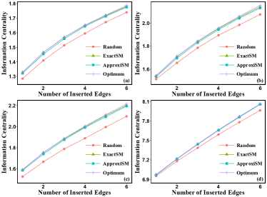
Figure 1: Average information centrality of target nodes as a function of the number $k$ of inserted edges for ExactSM, ApproxiSM, random and the optimum solution on four networks: BA (a), WS (b), Karate club (c), and Windsufers (d).

To further demonstrate effectiveness of our algorithms, we compare the results of our methods with the random scheme and other two baseline schemes, Top-degree and Top-cent, on four other real-world networks. In Top-degree scheme, the added edges are simply the $k$ edges connecting target node $v$ and its nonadjacent nodes with the highest degree in the original network; while in Top-cent scheme, the added edges are simply those $k$ edges connecting target node $v$ and its nonadjacent nodes with the largest information centrality in the original network.

Since the results may vary depending on the initial information centrality of the target node $v$, for each of the four real networks, we select 10 different target nodes at random. For each target node, we first compute its original information centrality and increase it by adding up to $k=20$ new edges, using our two greedy algorithms and the three baselines. Then, we compute and record the information centrality of the target node after insertion of every edge. Finally, we compute the average information centrality of all the 10 target nodes for each $k=1,2,\ldots,20$, which is plotted in Figure 2. We observe that for all the four real-world networks our greedy algorithms outperform the three baselines.

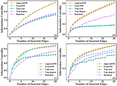
Figure 2: Average information centrality of target nodes as a function of the number $k$ of inserted edges for the five heuristics on Jazz musicians (a), Euroroad (b), Facebook (c), Powergrid (d).

7.2 Efficiency Comparison of Greedy Algorithms

Although both of our greedy algorithms are effective, we will show that their efficiency greatly differs. To this end, we compare the efficiency of the greedy algorithms on several real-world networks. For each network, we choose stochastically 20 target nodes, for each of which, we create $k=10$ new edges incident to it to maximize its information centrality according to Algorithms 1 and 3. We compute the average information centrality of 10 target nodes for each network and record the average running times. In Table 2 we provide the results of average information centrality and average running time of our greedy algorithms. We observe that ApproxiSM algorithm are faster than ExactSM algorithm, especially for large networks, while their final information centrality score are close. More interestingly, ApproxiSM applies to massive networks. For example, for com-DBLP and roadNet-TX networks, ApproxiSM computes their information centrality in half an hour, while ApproxiSM fails due to its high time complexity.

Table 2: The average running times and results of ApproxiSM (ASM) and ExactSM (ESM) algorithms on several real-world networks, as well as the ratios for times and results of ApproxiSM to those of ExactSM.

Network	Time (seconds)			Information centrality
	ASM	ESM	Ratio	ASM	ESM	Ratio
Virgili	1.3996	0.9172	1.5259	2.5005	2.5037	0.9987
Euroroad	0.6563	0.7593	0.8643	0.4003	0.4069	0.9838
Hamster full	3.0785	4.8528	0.6344	2.9904	2.9944	0.9987
Facebook	1.7151	12.9203	0.1327	0.7937	0.7947	0.9987
Powergrid	5.8727	58.3359	0.1006	0.4327	0.4369	0.9904
ca-GrQc	5.3023	34.0228	0.1558	1.2118	1.2136	0.9985
ca-HepPh	28.7462	620.4557	0.0463	2.2569	2.2592	0.9990
com-DBLP	697.1835	-	-	1.1327	-	-
roadNet-TX	1569.5059	-	-	0.0556	-	-

8 Conclusions

In this paper, we considered the problem of maximizing the information centrality of a designated node $v$ by adding $k$ new edges incident to it. This problem is equivalent to minimizing the resistance distance $\mathcal{R}_{v}$ of node $v$. We proposed two approximation algorithms for computing $\mathcal{R}_{v}$ when $k$ edges are repeatedly inserted in a greedy way. The first one gives a $\left(1-\frac{1}{e}\right)$ approximation of the optimum in time $O(n^{3})$. While the second one returns a $\left(1-\frac{1}{e}-\epsilon\right)$ approximation in time $\mathaccent 869{O}(mk\epsilon^{-2})$. Since the considered problem has never addressed before, we have no other algorithms to compare with, but compare our algorithms with potential alternative algorithms. Extensive experimental results on model and realistic networks show that our algorithms can often compute an approximate optimal solution. Particularly, our second algorithm can achieve a good approximate solution very quickly, making it applicable to massive networks.

References

- Avrachenkov and Litvak (2006) K. Avrachenkov and N. Litvak. The effect of new links on Google PageRank. Stochastic Models, 22(2):319–331, 2006.
- Avron and Toledo (2011) H. Avron and S. Toledo. Randomized algorithms for estimating the trace of an implicit symmetric positive semi-definite matrix. Journal of ACM, 58(2):8:1–8:34, 2011.
- Badanidiyuru and Vondrák (2014) A. Badanidiyuru and J. Vondrák. Fast algorithms for maximizing submodular functions. In SODA, pages 1497–1514. SIAM, 2014.
- Bergamini et al. (2016) E. Bergamini, M. Wegner, D. Lukarski, and H. Meyerhenke. Estimating current-flow closeness centrality with a multigrid Laplacian solver. In CSC, pages 1–12, 2016.
- Boldi and Vigna (2014) P. Boldi and S. Vigna. Axioms for centrality. Internet Mathematics, 10(3-4):222–262, 2014.
- Bozzo and Franceschet (2013) E. Bozzo and M. Franceschet. Resistance distance, closeness, and betweenness. Social Networks, 35(3):460–469, 2013.
- Brandes and Fleischer (2005) U. Brandes and D. Fleischer. Centrality measures based on current flow. In STACS, volume 3404, pages 533–544. Springer-Verlag, 2005.
- Crescenzi et al. (2015) P. Crescenzi, G. D’Angelo, L. Severini, and Y. Velaj. Greedily improving our own centrality in a network. In SEA, pages 43–55. Springer, 2015.
- Crescenzi et al. (2016) P. Crescenzi, G. D’Angelo, L. Severini, and Y. Velaj. Greedily improving our own closeness centrality in a network. ACM Transactions on Knowledge Discovery from Data, 11(1):9, 2016.
- D’Angelo et al. (2016) G. D’Angelo, L. Severini, and Y. Velaj. On the maximum betweenness improvement problem. Electronic Notes in Theoretical Computer Science, 322:153–168, 2016.
- Demaine and Zadimoghaddam (2010) E. D. Demaine and M. Zadimoghaddam. Minimizing the diameter of a network using shortcut edges. In SWAT, pages 420–431. Springer-Verlag, 2010.
- Doyle and Snell (1984) P. G. Doyle and J. L. Snell. Random Walks and Electric Networks. Mathematical Association of America, 1984.
- Hoffmann et al. (2018) C. Hoffmann, H. Molter, and M. Sorge. The parameterized complexity of centrality improvement in networks. In SOFSEM, pages 111–124. Springer, 2018.
- Hutchinson (1989) M. F. Hutchinson. A stochastic estimator of the trace of the influence matrix for Laplacian smoothing splines. Communications in Statistics-Simulation and Computation, 18(3):1059–1076, 1989.
- Ishakian et al. (2012) V. Ishakian, D. Erdös, E. Terzi, and A. Bestavros. A framework for the evaluation and management of network centrality. In SDM, pages 427–438. SIAM, 2012.
- Izmailian et al. (2013) N. Sh Izmailian, R. Kenna, and FY Wu. The two-point resistance of a resistor network: a new formulation and application to the cobweb network. Journal of Physics A: Mathematical and Theoretical, 47(3):035003, 2013.
- Klein and Randić (1993) D. J Klein and M. Randić. Resistance distance. Journal of Mathematical Chemistry, 12(1):81–95, 1993.
- Kunegis (2013) J. Kunegis. Konect: the koblenz network collection. In WWW, pages 1343–1350. ACM, 2013.
- Kyng and Sachdeva (2016) R. Kyng and S. Sachdeva. Approximate Gaussian elimination for Laplacians-fast, sparse, and simple. In FOCS, pages 573–582. IEEE, 2016.
- Lü et al. (2016) L Lü, D Chen, X Ren, Q Zhang, Y Zhang, and T Zhou. Vital nodes identification in complex networks. Physics Reports, 650:1–63, 2016.
- Meyer (1973) C. D. Meyer, Jr. Generalized inversion of modified matrices. SIAM Journal on Applied Mathematics, 24(3):315–323, 1973.
- Meyerson and Tagiku (2009) A. Meyerson and B. Tagiku. Minimizing average shortest path distances via shortcut edge addition. APPROX, pages 272–285. Springer-Verlag 2009.
- Nemhauser et al. (1978) G. L. Nemhauser, L. A. Wolsey, and M. L. Fisher. An analysis of approximations for maximizing submodular set functions. Mathematical Programming, 14(1):265–294, 1978.
- Newman (2005) M. E. J. Newman. A measure of betweenness centrality based on random walks. Social Networks, 27(1):39–54, 2005.
- Newman (2010) M. E. J. Newman. Networks: An Introduction. Oxford University Press, 2010.
- Olsen (2010) M. Olsen. Maximizing PageRank with new backlinks. In ICAC, pages 37–48. Springer-Verlag, 2010.
- Parotsidis et al. (2016) N. Parotsidis, E. Pitoura, and P. Tsaparas. Centrality-aware link recommendations. In WSDM, pages 503–512. ACM, 2016.
- Peng and Spielman (2014) R. Peng and D. A Spielman. An efficient parallel solver for SDD linear systems. In STOC, pages 333–342. ACM, 2014.
- Plemmons (1977) R. J. Plemmons. M-matrix characterizations. I nonsingular M-matrices. Linear Algebra and its Applications, 18(2):175–188, 1977.
- Spielman and Srivastava (2011) D. A. Spielman and N. Srivastava. Graph sparsification by effective resistances. SIAM Journal of Computing, 40(6):1913–1926, 2011.
- Stephenson and Zelen (1989) K. Stephenson and M. Zelen. Rethinking centrality: Methods and examples. Social Networks, 11(1):1–37, 1989.
- White and Smyth (2003) S. White and P. Smyth. Algorithms for estimating relative importance in networks. In KDD, pages 266–275. ACM, 2003.