Photorefractive second-harmonic detection for ultrasound-modulated optical tomography

Abstract

Ultrasound-modulated optical tomography enables sharp 3D optical imaging of tissues and other turbid media, but the light modulation signals are hard to sensitively measure. A common solution, involving photorefractive crystals, enables the measurement of a relatively slow and low-spatial-resolution signal tracking the envelope of the ultrasound wave. We reexamine the photorefractive detection principle both intuitively and quantitatively, and from this analysis we predict that the photodetector should additionally see a fast response at twice the ultrasound frequency, and correspondingly high spatial frequency. The fast and slow response usually have similar amplitudes and reveal complementary information, thus allowing ultrasound-modulated optical tomography to create dramatically sharper tomographic images under the same measurement conditions, integration time, and experimental complexity.

1 Introduction

Ultrasound-modulated optical tomography [1], also called acousto-optic tomography or acousto-optic imaging, is an emerging medical imaging technology promising a uniquely appealing combination of features, including high spatial resolution ($<1\text{mm}{}^{3}$), deep penetration ($\gg 1\text{cm}$), sensitivity to visible texture (light scattering and refractive index contrast, unlike photoacoustic tomography which is limited to light absorption contrast), excellent safety profile (non-invasive, no contrast agents, no ionizing radiation), and a path to low-cost, even portable, equipment.

In ultrasound-modulated optical tomography, one sends laser light (typically near-infrared) and ultrasound simultaneously into a tissue. The two waves interact inside the tissue (Sec. 2.1 below), with the effect that the light exiting the tissue is amplitude-modulated and phase-modulated at the ultrasound frequency. The amount of light modulation is the signal to be measured in this technique. This modulation signal is especially useful because it inherits the spatial resolution of ultrasound—which for example can be focused to small points deep inside the tissue and scanned around—while still maintaining the image contrast of light, including distinguishing subtle properties of soft tissues without contrast agents, and measuring blood volume, flow, and oxygenation. Light by itself (diffuse optical tomography) has comparatively poor spatial resolution because of scattering by the tissue—to get appreciable depth, it is often necessary to use photons that have been scattered hundreds of times inside the tissue.

One of the principal challenges in implementing ultrasound-modulated optical tomography is detecting the light modulation signal. Unfortunately, light exits the tissue in a diffuse, high-étendue, laser speckle pattern. Thus the most naive approach—collecting lots of light into a large-area fast detector, and watching its output for modulation at the ultrasound frequency—works quite poorly. There are many speckles entering the detector, and they are modulated with different phases, with some getting brighter at the same time as others are getting dimmer, and thus the speckles largely cancel each other out.

To work around this issue, a wide variety of alternative approaches have been explored, including small detectors [2], CCD or CMOS imaging detectors [3], narrowband filters [4, 5], and many others [1]. However, challenges remain in combining very high detector étendue (i.e. collecting many photons), reasonable cost and convenience, high SNR, and compatibility with fast, high-bandwidth measurements, such as in Ref. [6].

One of the most promising and widely-used detection methods is photorefractive detection [7, 8, 9, 10], as shown in Fig. 1. In this technique, the outgoing speckle pattern passes through a photorefractive crystal. Meanwhile a “reference beam” light source passes through the same photorefractive crystal. In the configuration we discuss in this paper, the reference beam is at the same frequency as the laser illuminating the tissue. (This is not the only possible photorefractive detection configuration [8, 11], but it is most appropriate for fast, high-bandwidth measurements.) As discussed below, the reference beam and the speckle pattern undergo two-wave mixing, and this leads to a signal indicating the amount of ultrasound modulation. In photorefractive detection, unlike the naive approach mentioned above, the different speckles do not cancel each other out, and therefore a large-area detector can be used without reducing the relative strength of the modulation signal.

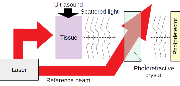
Figure 1: (a) Schematic block diagram of the photorefractive detection system. A CW laser illuminates a tissue, creating a speckle pattern of scattered light. This is overlapped with a reference beam in a photorefractive crystal, and then a photodetector integrates the total light power received.

In previous work [12, 8, 6], photorefractive detection has been treated as having a spatial resolution equal to the envelope of the ultrasound wave. We will argue that if a faster optical detector is used (much faster than the ultrasound frequency), then the spatial resolution has much finer structure, as in Fig. 2, associated with oscillations at the second harmonic of the ultrasound frequency. In many situations, these signals are beneficial to measure: they can reveal very small features and sharp edges (see Fig. 2); higher-frequency signals are often easier to detect over background; higher-frequency signals offer more data channels per unit time; the fast and slow signals can be measured simultaneously with little extra effort, enabling measurement of both large-scale and small-scale structure; and for technical reasons discussed below, the high-frequency signal can sometimes have a somewhat different image contrast than the low-frequncy signal, such that we can make certain features stand out (Sec. 4 below).

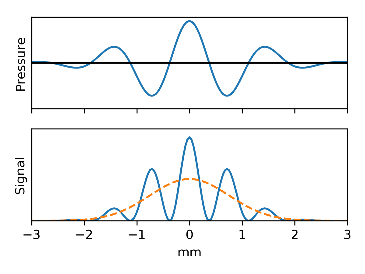
Figure 2: Top: An example ultrasound waveform, showing a snapshot of a short pulse at 1MHz with $v_{\text{sound}}=1.5\text{km}/\text{s}$, as it travels through the medium. Bottom: If this wave is used for ultrasound-modulated optical tomography with photorefractive detection, under typical operating conditions (Sec. 2.1), we will argue that the spatial sensitivity at each moment is approximately as shown by the solid blue line. If the detector is too slow to measure the fast oscillations, the spatial sensitivity would instead be the dashed line, as in previous work.

1.1 Nonlinear modulation vs. nonlinear detection

Photorefractive detection, as we describe it here, involves the nonlinear detection of a linear acousto-optic modulation signal, and we will find that the second-harmonic signal discussed in this paper appears in the lowest order of perturbation theory. This topic should thus be distinguished from nonlinear modulation of light in the tissue. Examples of the latter include purely acoustic second-harmonic generation—when the acoustic amplitude is sufficiently strong that the tissue’s mechanical response is anharmonic—or acousto-optic second-harmonic generation—when the acousto-optic interaction is sufficiently strong that the light modulation is anharmonic. Example of nonlinear modulation include Refs. [13, 14], in which second-harmonic signals in ultrasound-modulated optical tomography were seen in CCD-based measurements.

Nonlinear modulation offers intriguing potential applications, particularly with focused ultrasound, but is weaker than the main signal at the ultrasound frequency. Photorefractive detection offers an exciting avenue because, regardless of ultrasound intensity, we predict a second-harmonic signal with similar amplitude to the slow envelope signal—and experience shows that the latter can be measured even at high speeds with unfocused beams [6].

To the extent that nonlinear modulation occurs, a photorefractive detector would see it as a fourth harmonic signal.

2 Qualitative explanation

2.1 Index effect vs. displacement effect

We predict that the strength and presence of the second-harmonic signal depends critically on the phase relation between an ultrasound wave and the optical modulation it induces. Having a consistent, predictable phase relation is critical to ensuring that the signal adds coherently, rather than randomly, over all the different light paths meandering through the highly-scattering tissue.

Previous work [15, 16] has identified two mechanisms by which ultrasound modulates light, each with a different phase relation. The first mechanism is the index effect, wherein the pressure of the sound wave changes the refractive index of the water in the tissue (piezo-optic effect), which in turn changes the optical phase of light passing through that region of tissue. The second is the displacement effect, where the light-scattering structures in the tissue move back and forth at the ultrasound frequency.

As shown in Fig. 3, the two mechanisms lead to different optical modulation phases, and indeed, if both are present equally, they tend to create equal and opposite second-harmonic signals that cancel out in a photorefractive detection system.

However, for typical tissue parameters and ultrasound frequencies, the two mechanisms are not present equally; instead, the index effect predominates over the displacement effect [15, 16]. For example, for tissue with light scattering coefficient $1\text{mm}^{-1}$, the index effect is predicted to account for $\frac{2}{3}$ of the total light modulation with 500kHz ultrasound, $\frac{3}{4}$ with 1MHz ultrasound, and increasing towards 100% at higher frequency. (More generally, for water-based media, the index effect predominates by at least a 2:1 ratio on condition that the ultrasound wavelength $\lambda_{\text{US}}<2l$, where $l$ is the mean free path for photon scattering [15, 16].)

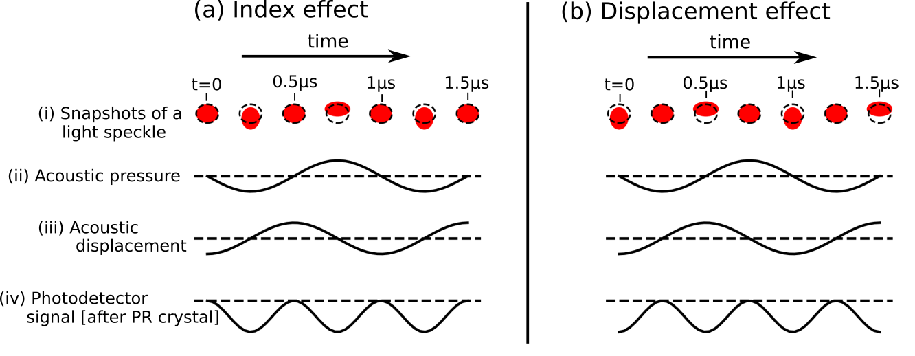
Figure 3: Schematic depiction of speckle modulation during 1.5 ultrasound cycles, with ultrasound frequency 1MHz, showing (i) a series of snapshots of a representative laser speckle exiting the tissue at different times, (ii) the acoustic pressure and (iii) displacement at the part of the tissue causing this modulation, and (iv) the photodetector signal after the photorefractive crystal. In all cases, dashed lines indicate the equilibrium with no ultrasound. (a) If the light modulation is caused by the index effect (Sec. 2.1), the light speckle changes in phase with the pressure—i.e. when pressure is at its equilibrium value, the speckle is in its equilibrium position; (b) If the light modulation is instead caused by the displacement effect, the light speckles change in phase with the displacement. Either way, as explained in Sec. 2.3, the signal (iv) shrinks when the speckles (i) are displaced from their time-averaged configuration.

2.2 Two-wave mixing

A photorefractive crystal has the defining property that the crystal’s refractive index changes in response to how much light intensity is at any given point. This gives rise to “two-wave mixing” [17, 18, 8, 19]. In this phenomenon, two light beams of the same wavelength shine into the crystal. The interference pattern between these two beams produces peaks and nulls of intensity within the crystal, which in turn creates a volumetric diffraction grating in the crystal. This grating diffracts each beam into the spatial mode of the other beam. In this case, one of the “beams” is a complicated laser speckle pattern, but the principle still works: the volume grating diffracts light from the reference beam into the complicated laser speckle spatial profile, and vice-versa.

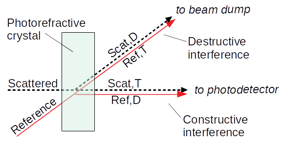
Figure 4: Zoomed-in diagram of the photorefractive crystal of Fig. 1. The four beams exiting the crystal on the right are, from top to bottom, the diffracted scattered light, the transmitted reference beam, the transmitted scattered light, and the diffracted reference beam. The labels “destructive interference” and “constructive interference” are as discussed in Sec. 2.2.

Referring to Fig. 4, there is interference between the diffracted reference beam and the transmitted scattered light traveling to the photodetector, and there is also interference between the transmitted reference beam and diffracted scattered light traveling to the beam dump. For definiteness, we will assume that the former interference is constructive, and hence (by conservation of energy) that the latter interference is destructive. This case corresponds to positive gain for the scattered light, i.e. transfer of power from the reference to the scattered light paths. In general, the sign of gain, and correspondingly the choice of which of the beams is amplified and which is depleted, depends on the detailed mechanism of photorefraction, including the crystallographic axis, beam propagation directions, and direction of the electric field applied across the crystal (if any) [20]. If we instead made the opposite assumption, i.e. transfer of power into the reference beam, the system would still work, but some signs would be flipped in the discussion below, e.g. the presence of ultrasound would tend to increase, rather than decrease, the photodetector signal.

What makes two-wave mixing particularly useful for our purposes is that the crystal’s photorefractive response time, $\tau_{\text{PR}}$, is much slower than the ultrasound frequency. Therefore the diffracted reference beam is not quite a copy of the speckle pattern exiting the tissue, but rather a time-averaged copy of that speckle pattern. This is shown schematically in Fig. 3(i), where a representative speckle exiting the tissue (red dot) is modulated, while the corresponding diffracted speckle from the reference beam (dashed line) stays stationary. The time-averaged copy enables “change detection” for the light: We are essentially comparing the speckle pattern to its time-averaged copy, and if they are very different, we infer that the light is being strongly modulated by the ultrasound.

2.3 Mode overlap determines output signal

A key aspect of the photorefractive detection method is the interference between the transmitted scattered light and the diffracted reference beam. Each beam by itself has an approximately fixed total power, but to the extent that the two beams interfere, it sends more power to the photodetector and less power to the beam dump (Fig. 4).

If both beams are static for a long time compared to $\tau_{\text{PR}}$, then a properly-configured photorefractive crystal will naturally develop an index profile that maximizes interference, such that the beams are maximally in phase and overlapped. This maximizes the power to the photodetector, and minimizes the signal to the beam dump of Fig. 4. However, if the scattered light is modulated by the ultrasound, its phase and amplitude profile will not perfectly match the diffracted reference beam, so the interference will be less effective, and the photodetector will see less light. This phenomenon is part of Fig. 3: the more the speckles are altered from their time-averaged pattern (Fig. 3(i)), the less power is detected (Fig. 3(iv)).

As stated above, two interfering waves convey maximum power when they are in phase and have matching spatial profiles. This familiar fact from wave mechanics can be mathematically proven by writing [8]:

Photodetector signal $$=\int d^{2}\mathbf{r}\left|\mathscr{E}_{S}(\mathbf{r})+\mathscr{E}_{D}(\mathbf{r})\right|^{2}$$

$$=C+2\int d^{2}\mathbf{r}\text{Re}\left[\mathscr{E}_{S}^{*}(\mathbf{r})\mathscr{E}_{D}(\mathbf{r})\right]$$ (1)

where $\text{Re}\left[\mathscr{E}_{S}(\mathbf{r})e^{-i\omega_{0}t}\right]$ is the electric field of the transmitted scattered light in Fig. 4; $\text{Re}\left[\mathscr{E}_{D}(\mathbf{r})e^{-i\omega_{0}t}\right]$ is the electric field of the diffracted reference beam in Fig. 4; and $C\equiv\int d^{2}\mathbf{r}\left|\mathscr{E}_{S}(\mathbf{r})\right|^{2}+\int d^{2}\mathbf{r}\left|\mathscr{E}_{D}(\mathbf{r})\right|^{2}$ is a constant approximately independent of the presence or absence of ultrasound. Now we invoke the Cauchy–Schwarz inequality:

$$\int d^{2}\mathbf{r}\text{Re}\left[\mathscr{E}_{S}^{*}(\mathbf{r})\mathscr{E}_{D}(\mathbf{r})\right]=\sqrt{\int d^{2}\mathbf{r}\left|\mathscr{E}_{S}^{2}(\mathbf{r})\right|\cdot\int d^{2}\mathbf{r}\left|\mathscr{E}_{D}^{2}(\mathbf{r})\right|}\\ \text{if }\mathscr{E}_{S}\text{ \& }\mathscr{E}_{D}\text{ have the same phase \& spatial mode}$$ (2a)

$$\int d^{2}\mathbf{r}\text{Re}\left[\mathscr{E}_{S}^{*}(\mathbf{r})\mathscr{E}_{D}(\mathbf{r})\right]<\sqrt{\int d^{2}\mathbf{r}\left|\mathscr{E}_{S}^{2}(\mathbf{r})\right|\cdot\int d^{2}\mathbf{r}\left|\mathscr{E}_{D}^{2}(\mathbf{r})\right|}\\ \text{otherwise}$$ (2b)

If $\mathscr{E}_{S}$ and $\mathscr{E}_{D}$ have the same phase profile and spatial mode, i.e. if $\frac{\mathscr{E}_{S}(\mathbf{r})}{\mathscr{E}_{D}(\mathbf{r})}$ is the same positive constant everywhere, then the photodetector signal is maximized. If $\mathscr{E}_{S}$ and $\mathscr{E}_{D}$ are mis-matched at all, the photodetector signal goes down.

As shown in Fig. 3(iv), the presence of ultrasound both decreases the time-averaged photodetector signal, and causes a fast modulation at twice the ultrasound frequency. The former is the familiar slow signal whose spatial sensitivity tracks the envelope of the ultrasound wave; the latter is the subject of this article.

3 Quantitative derivation

As above, we say $\omega_{0}$ is the laser frequency and $\omega_{\text{US}}$ is the ultrasound frequency (assumed monochromatic for simplicity). We write the scattered field (i.e. the speckle pattern coming out of the tissue) as $\text{Re}\left(\mathscr{E}_{S}(\mathbf{r}_{e},t)e^{-i\omega_{0}t}\right)$, where $\mathscr{E}_{S}$ is a complex amplitude and $\mathbf{r}_{e}$ is any point in the exterior of the tissue where the light exits as a speckle pattern. It will be most convenient to set $\mathbf{r}_{e}$ to points on the photodetector surface, in which case $\mathscr{E}_{S}$ incorporates the effects of passing the photorefractive crystal, i.e. some absorptive and diffractive loss, both usually small in practice [8]. To simplify the descriptions, we neglect speckle decorrelation, i.e. we assume that $\mathscr{E}_{S}(\mathbf{r}_{e},t)$ depends on time only because of the presence of ultrasound, and not because of blood flow or other motion. (Photorefractive detection continues to work in the presence of speckle decorrelation, but the signal strength goes down when the speckle decorrelation time is shorter than the photorefractive response time $\tau_{\text{PR}}$. In practice, sub-millisecond values of $\tau_{\text{PR}}$ are known to be feasible [21], and this is sufficiently low for most in vivo applications.)

The ultrasound wave inside the tissue creates local pressure change $P(\mathbf{r}_{i},t)$ and local displacement $D(\mathbf{r}_{i},t)$, where $t$ is time and $\mathbf{r}_{i}$ is a point inside the tissue. For example, a plane wave would have $P(\mathbf{r}_{i},t)=P_{0}\cos\left(\mathbf{k}\cdot\mathbf{r}_{i}-\omega_{\text{US}}t\right)$, $D(\mathbf{r}_{i},t)=\frac{P_{0}}{Z_{\text{US}}\omega_{\text{US}}}\sin\left(\mathbf{k}\cdot\mathbf{r}_{i}-\omega_{\text{US}}t\right)$, where $Z_{\text{US}}$ is the specific acoustic impedance (note that the displacement is $90^{\circ}$ out of phase with the pressure change). Then the effect of the ultrasound can be written using Green’s functions as:

$$\mathscr{E}_{S}(\mathbf{r}_{e},t) =\mathscr{E}_{S,0}(\mathbf{r}_{e},t)$$

$$\;+\,\int d^{3}\mathbf{r}_{i}G_{n}(\mathbf{r}_{i},\mathbf{r}_{e})P(\mathbf{r}_{i},t)+\int d^{3}\mathbf{r}_{i}G_{d}(\mathbf{r}_{i},\mathbf{r}_{e})D(\mathbf{r}_{i},t)$$ (3)

where $\mathscr{E}_{S,0}$ is the field in the absence of ultrasound; $G_{n}$ is the index-effect Green’s function, defined such that a unit change of pressure at the point $\mathbf{r}_{i}$ in the tissue causes an optical field amplitude change of $G_{n}(\mathbf{r}_{i},\mathbf{r}_{e})$ in the speckle pattern, at the point $\mathbf{r}_{e}$ external to the tissue; and $G_{d}$ is the displacement-effect Green’s function defined analogously. Eq. (3) is a first-order approximation, i.e. assuming that the ultrasound only modestly changes the light flow patterns. This is usually reasonable, and see Sec. 1.1 for further discussion. As mentioned above, we are ignoring blood flow and other motion, so $G_{n}$ and $G_{d}$ do not depend on time.

If we did not have a photorefractive crystal and reference beam, but instead just sent the scattered light into a single-pixel large-area photodetector, it would register an intensity fluctuation of:

$$\Delta I(t) \equiv\int d^{2}\mathbf{r}_{e}\left(\left|\mathscr{E}_{S}(\mathbf{r}_{e},t)\right|^{2}-\left|\mathscr{E}_{S,0}(\mathbf{r}_{e})\right|^{2}\right)$$

$$=\int d^{2}\mathbf{r}_{e}\left(2\text{Re}\left[\mathscr{E}_{S,0}^{*}(\mathbf{r}_{e})\int d^{3}\mathbf{r}_{i}\left(G_{n}(\mathbf{r}_{i},\mathbf{r}_{e})P(\mathbf{r}_{i},t)\right)\right]\right)$$

$$\quad+\int d^{2}\mathbf{r}_{e}\left(2\text{Re}\left[\mathscr{E}_{S,0}^{*}(\mathbf{r}_{e})\int d^{3}\mathbf{r}_{i}\left(G_{d}(\mathbf{r}_{i},\mathbf{r}_{e})D(\mathbf{r}_{i},t)\right)\right]\right)$$

$$\quad+\int d^{2}\mathbf{r}_{e}\left|\int d^{3}\mathbf{r}_{i}\left(G_{n}(\mathbf{r}_{i},\mathbf{r}_{e})P(\mathbf{r}_{i},t)+G_{d}(\mathbf{r}_{i},\mathbf{r}_{e})D(\mathbf{r}_{i},t)\right)\right|^{2}$$

As discussed in Sec. 1, this fluctuation $\Delta I$ is quite small: The ultrasound slightly changes photon phases and paths, but does not systematically change the total flux of photons exiting the tissue into the large detector area. (Indeed, if this modulation were not so small, there would be no need for the photorefractive crystal!)

As described in [8] (see also Eq. (1)), under typical experimental conditions, the photodetector measures a quantity proportional to:

$$\text{Signal}(t)=\int d^{2}\mathbf{r}_{e}\left(2\text{Re}\left[\mathscr{E}_{S,0}^{*}(\mathbf{r}_{e})\mathscr{E}_{S}(\mathbf{r}_{e},t)\right]\right)$$ (4)

where $\mathscr{E}_{S,0}$ is proportional to the diffracted reference beam (Fig. 4), which imitates a time-averaged version of the scattered light speckle pattern $\mathscr{E}_{S}$ (Sec. 2.2).

In Eq. (4), there is a time-independent and ultrasound-independent offset of $2\int\left|\mathscr{E}_{S,0}\right|^{2}$, which can be experimentally subtracted off by, for example, comparing the signal with and without ultrasound [8]. Discarding that, we are left with:

$$\text{Signal}(t)=\Delta I(t)-\int d^{2}\mathbf{r}_{e}\left|\int d^{3}\mathbf{r}_{i}\left(G_{n}(\mathbf{r}_{i},\mathbf{r}_{e})P(\mathbf{r}_{i},t)\right.\right.\\ \left.+G_{d}(\mathbf{r}_{i},\mathbf{r}_{e})D(\mathbf{r}_{i},t)\right)\Big{|}^{2}$$

To simplify this, first we ignore the small quantity $\Delta I(t)$, then we note that the quantities $G_{n}(\mathbf{r}_{i},\mathbf{r}_{e})$ and $G_{d}(\mathbf{r}_{i}^{\prime},\mathbf{r}_{e}^{\prime})$ are statistically uncorrelated (have a random phase relation). This leads to:

$$\left\langle\text{Signal}(t)\right\rangle=\left\langle-\int d^{2}\mathbf{r}_{e}\left|\int d^{3}\mathbf{r}_{i}G_{n}(\mathbf{r}_{i},\mathbf{r}_{e})P(\mathbf{r}_{i},t)\right|^{2}\right.\\ \left.-\int d^{2}\mathbf{r}_{e}\left|\int d^{3}\mathbf{r}_{i}G_{d}(\mathbf{r}_{i},\mathbf{r}_{e})D(\mathbf{r}_{i},t)\right|^{2}\right\rangle$$

Next we try to simplify:

$$\left|\int d^{3}\mathbf{r}_{i}G_{n}(\mathbf{r}_{i},\mathbf{r}_{e})P(\mathbf{r}_{i},t)\right|^{2}\\ =\int d^{3}\mathbf{r}_{i}\int d^{3}\mathbf{r}_{i}^{\prime}G_{n}(\mathbf{r}_{i},\mathbf{r}_{e})P(\mathbf{r}_{i},t)G_{n}^{*}(\mathbf{r}_{i}^{\prime},\mathbf{r}_{e})P(\mathbf{r}_{i}^{\prime},t)$$

Under typical circumstances, the statistical correlation between $G_{n}(\mathbf{r}_{i},\mathbf{r}_{e})$ and $G_{n}(\mathbf{r}_{i}^{\prime},\mathbf{r}_{e})$ smoothly decays to zero with increasing $\left|\mathbf{r}_{i}-\mathbf{r}_{i}^{\prime}\right|$, which leads to:

$$\left\langle\left|\int d^{3}\mathbf{r}_{i}G_{n}(\mathbf{r}_{i},\mathbf{r}_{e})P(\mathbf{r}_{i},t)\right|^{2}\right\rangle=B_{n}\int d^{3}\mathbf{r}_{i}\left\langle\left|G_{n}(\mathbf{r}_{i},\mathbf{r}_{e})\right|^{2}\right\rangle P^{2}(\mathbf{r}_{i},t)$$

where $B_{n}=\frac{\int d^{3}\mathbf{r}_{i}^{\prime}P(\mathbf{r}_{i}^{\prime})\left\langle G_{n}(\mathbf{r}_{i},\mathbf{r}_{e})G_{n}^{*}(\mathbf{r}_{i}^{\prime},\mathbf{r}_{e})\right\rangle}{P(\mathbf{r}_{i})\left\langle\left|G_{n}(\mathbf{r}_{i},\mathbf{r}_{e})\right|^{2}\right\rangle}$ is roughly the ratio of ultrasound pressure averaged over a sphere centered at a point to pressure at the center of that sphere, where the sphere size corresponds to the autocorrelation length of $G_{n}$ mentioned above. If the ultrasound waveform is approximately sinusoidal, $B_{n}$ will be approximately the same real constant at each point $\mathbf{r}_{i}$, although the constant will vary with ultrasound frequency, scattering coefficient, and other parameters. The $G_{d}$ case is similar, so the end result is:

$$\left\langle\text{Signal}(t)\right\rangle\propto-\int d^{2}\mathbf{r}_{e}\int d^{3}\mathbf{r}_{i}\left(B_{n}\left\langle\left|G_{n}(\mathbf{r}_{i},\mathbf{r}_{e})\right|^{2}\right\rangle P^{2}(\mathbf{r}_{i},t)\right.\\ \left.+\,B_{d}\left\langle\left|G_{d}(\mathbf{r}_{i},\mathbf{r}_{e})\right|^{2}\right\rangle D^{2}(\mathbf{r}_{i},t)\right)$$

Define the total modulation $M$ ($M_{n}$ for index effect and $M_{d}$ for displacement effect) by

$$M_{n}(\mathbf{r}_{i})\equiv B_{n}\int d^{2}\mathbf{r}_{e}\left\langle\left|G_{n}(\mathbf{r}_{i},\mathbf{r}_{e})\right|^{2}\right\rangle$$

$$M_{d}(\mathbf{r}_{i})\equiv B_{d}\int d^{2}\mathbf{r}_{e}\left\langle\left|G_{d}(\mathbf{r}_{i},\mathbf{r}_{e})\right|^{2}\right\rangle$$

Mapping these quantities is an end-goal of ultrasound-modulated optical tomography, as they reveal information about how much light passes through each point $\mathbf{r}_{i}$, how much light scattering is happening at that point, how much water content is at that point, and so on. We have:

$$\left\langle\text{Signal}(t)\right\rangle\propto-\int d^{3}\mathbf{r}_{i}\left(M_{n}(\mathbf{r}_{i})P^{2}(\mathbf{r}_{i},t)+M_{d}(\mathbf{r}_{i})D^{2}(\mathbf{r}_{i},t)\right)$$

Finally, we take the simple example of a monochromatic ultrasound plane wave in a uniform infinite medium: $P(\mathbf{r}_{i},t)=P_{0}\cos\left(\mathbf{k}\cdot\mathbf{r}_{i}-\omega_{\text{US}}t\right)$ and $D(\mathbf{r}_{i},t)=\frac{P_{0}}{Z_{\text{US}}\omega_{\text{US}}}\sin\left(\mathbf{k}\cdot\mathbf{r}_{i}-\omega_{\text{US}}t\right)$. We find that our signal is related to the Fourier coefficients of $M$:

$$\frac{\left\langle\text{Signal}(t)\right\rangle}{P_{0}^{2}} \propto-\left(\tilde{M}_{n}(0)+\frac{1}{Z_{\text{US}}^{2}\omega_{\text{US}}^{2}}\tilde{M}_{d}(0)\right)$$

$$\;-\,\text{Re}\left[\left(\tilde{M}_{n}(2\mathbf{k})-\frac{1}{Z_{\text{US}}^{2}\omega_{\text{US}}^{2}}\tilde{M}_{d}(2\mathbf{k})\right)e^{-2i\omega_{\text{US}}t}\right]$$ (5)

The first term on the right side is more generally the difference-frequency term, which tracks the envelope of the ultrasound wave and has been frequently measured in the literature. The second term is the sum-frequency term, which measures higher spatial frequency, and appears at higher temporal frequency (up to twice the highest ultrasound frequency). In the usual circumstance that $M_{n}\gg\frac{1}{Z_{\text{US}}^{2}\omega_{\text{US}}^{2}}M_{d}$ (see Sec. 2.1), the fast term and slow term have inherently equal amplitudes, though the actual amplitude of each will depend on the amplitude of the corresponding Fourier component of the image. For example, in a tissue with no fine features or sharp edges (where “fine” and “sharp” are compared to the ultrasound wavelength), the fast signal would be much weaker than the slow signal; conversely, a tissue with large-scale uniformity but small-scale random texture would generally show a stronger fast signal than slow signal. On the other hand, when $M_{n}\approx\frac{1}{Z_{\text{US}}^{2}\omega_{\text{US}}^{2}}M_{d}$, as when the ultrasound wavelength is much larger than the optical scattering mean free path (see Sec. 2.1), then the fast signal is expected to be much weaker than the slow signal under most circumstances.

4 Conclusion

We have argued both qualitatively and quantitatively that photorefractive detection setups should generally see a fast signal at the second harmonic (or more generally, at sum frequencies) of the ultrasound waves in the tissue, which, like the slow (compared to the ultrasound frequency) envelope-related signal, arises at the lowest order of perturbation theory and adds coherently over all the collected speckles. Compared to the previously-discussed slow signal, the fast signal is different and complementary. In terms of spatial sensitivity, the fast signal measures high-spatial-frequency Fourier components, and thus is blind to large structures but sensitive to small features, fine texture, and sharp edges, while the slow signal is the opposite (see Fig. 2 for a comparison at 1MHz; the fast signal is sensitive to sub-millimeter structures while the slow signal is sensitive to several-millimeter structures and larger, along the direction of ultrasound propagation). In terms of signal frequency, the fast signal requires a faster photodetector and ADC (Nyquist rate of $4\times$ the highest ultrasound frequency), but should benefit from lower background, and more importantly the same apparatus should be able to measure both the fast and slow frequency bands simultaneously. In terms of contrast, the slow signal effectively measures the sum $\left(M_{n}+\frac{1}{Z_{\text{US}}^{2}\omega_{\text{US}}^{2}}M_{d}\right)$ while the fast signal measures the difference $\left(M_{n}-\frac{1}{Z_{\text{US}}^{2}\omega_{\text{US}}^{2}}M_{d}\right)$. These two will often be effectively the same (if $M_{n}\gg\frac{1}{Z_{\text{US}}^{2}\omega_{\text{US}}^{2}}M_{d}$, as when $\lambda_{\text{US}}$ is less than twice the mean free path for photon scattering [15, 16], as is typical in tissues). But in certain cases, the difference term offers intriguing sensing possibilities. For example, with low-frequency ultrasound, it may be possible to arrange for $M_{n}\approx\frac{1}{Z_{\text{US}}^{2}\omega_{\text{US}}^{2}}M_{d}$ throughout the translucent tissue, but $M_{n}\gg\frac{1}{Z_{\text{US}}^{2}\omega_{\text{US}}^{2}}M_{d}$ in a particular area with unusually little light scattering, such as a cyst full of relatively clear fluid. The high-frequency signal component should then show a bright cyst on a dark background.

In future work, we plan to experimentally test and explore the predictions herein.

Acknowledgement I thank all those who generously offered feedback and criticism of this work, especially (but not exclusively) Joseph Hollmann, Charles DiMarzio, Krish Kotru, and Jeffrey Korn.

References

- [1] J. Gunther and S. Andersson-Engels, “Review of current methods of acousto-optical tomography for biomedical applications,” \JournalTitleFrontiers of Optoelectronics 10, 211–238 (2017).
- [2] L. Wang, S. L. Jacques, and X. Zhao, “Continuous-wave ultrasonic modulation of scattered laser light to image objects in turbid media,” \JournalTitleOptics Letters 20, 629–631 (1995).
- [3] S. Lévêque, A. C. Boccara, M. Lebec, and H. Saint-Jalmes, “Ultrasonic tagging of photon paths in scattering media: parallel speckle modulation processing,” \JournalTitleOptics Letters 24, 181–183 (1999).
- [4] S. Sakadžić and L. V. Wang, “High-resolution ultrasound-modulated optical tomography in biological tissues,” \JournalTitleOptics Letters 29, 2770–2772 (2004).
- [5] Y. Li, P. Hemmer, C. Kim, H. Zhang, and L. V. Wang, “Detection of ultrasound-modulated diffuse photons using spectral-hole burning,” \JournalTitleOptics Express 16, 14862–14874 (2008).
- [6] J.-B. Laudereau, A. A. Grabar, M. Tanter, J.-L. Gennisson, and F. Ramaz, “Ultrafast acousto-optic imaging with ultrasonic plane waves,” \JournalTitleOptics Express 24, 3774–3789 (2016).
- [7] T. W. Murray, L. Sui, G. Maguluri, R. A. Roy, A. Nieva, F. Blonigen, and C. A. DiMarzio, “Detection of ultrasound-modulated photons in diffuse media using the photorefractive effect,” \JournalTitleOptics Letters 29, 2509–2511 (2004).
- [8] M. Gross, F. Ramaz, B. C. Forget, M. Atlan, A. C. Boccara, P. Delaye, and G. Roosen, “Theoretical description of the photorefractive detection of the ultrasound modulated photons in scattering media,” \JournalTitleOptics Express 13, 7097–7112 (2005).
- [9] M. Gross, M. Lesaffre, F. Ramaz, P. Delaye, G. Roosen, and A. C. Boccara, “Detection of the tagged or untagged photons in acousto-optic imaging of thick highly scattering media by photorefractive adaptive holography,” \JournalTitleThe European Physical Journal E 28, 173–182 (2009).
- [10] P. Lai, X. Xu, and L. V. Wang, “Ultrasound-modulated optical tomography at new depth,” \JournalTitleJournal of Biomedical Optics 17, 066006 (2012).
- [11] M. Lesaffre, S. Farahi, M. Gross, P. Delaye, A. C. Boccara, and F. Ramaz, “Acousto-optical coherence tomography using random phase jumps on ultrasound and light,” \JournalTitleOptics Express 17, 18211–18218 (2009).
- [12] L. Sui, R. A. Roy, C. A. DiMarzio, and T. W. Murray, “Imaging in diffuse media with pulsed-ultrasound-modulated light and the photorefractive effect,” \JournalTitleApplied Optics 44, 4041–4048 (2005).
- [13] J. Selb, L. Pottier, and A. C. Boccara, “Nonlinear effects in acousto-optic imaging,” \JournalTitleOptics Letters 27, 918 (2002).
- [14] H. Ruan, M. L. Mather, and S. P. Morgan, “Pulse inversion ultrasound modulated optical tomography,” \JournalTitleOptics Letters 37, 1658–1660 (2012).
- [15] L. V. Wang, “Mechanisms of ultrasonic modulation of multiply scattered coherent light: a Monte Carlo model,” \JournalTitleOptics Letters 26, 1191–1193 (2001).
- [16] L. V. Wang, “Mechanisms of ultrasonic modulation of multiply scattered coherent light: an analytic model,” \JournalTitlePhysical Review Letters 87, 043903 (2001).
- [17] P. Delaye, L. A. de Montmorillon, and G. Roosen, “Transmission of time modulated optical signals through an absorbing photorefractive crystal,” \JournalTitleOptics Communications 118, 154–164 (1995).
- [18] M. Chi, J.-P. Huignard, and P. M. Petersen, “A general theory of two-wave mixing in nonlinear media,” \JournalTitleJournal of the Optical Society of America B 26, 1578 (2009).
- [19] P. Yeh, Introduction to photorefractive nonlinear optics, Wiley series in pure and applied optics (Wiley, New York, 1993).
- [20] M. H. Garrett, J. Y. Chang, H. P. Jenssen, and C. Warde, “High beam-coupling gain and deep- and shallow-trap effects in cobalt-doped barium titanate, BaTiO:Co,” \JournalTitleJOSA B 9, 1407–1415 (1992).
- [21] M. Lesaffre, F. Jean, A. Bordes, F. Ramaz, E. Bossy, A. C. Boccara, M. Gross, P. Delaye, and G. Roosen, “Sub-millisecond in situ measurement of the photorefractive response in a self adaptive wavefront holography setup developed for acousto-optic imaging,” in “Photons Plus Ultrasound: Imaging and Sensing 2006: The Seventh Conference on Biomedical Thermoacoustics, Optoacoustics, and Acousto-optics,” , vol. 6086 (International Society for Optics and Photonics, 2006), vol. 6086, p. 608612.