1 Preface

1. From February 14-15, 2018, the Thomas Jefferson Laboratory in Newport News, Virginia hosted the PKI2018, an international workshop to explore the physics potential to investigate $\pi$-K interactions. This was the fourth of a series of workshops held to establish a neutral kaon beam facility at JLab Hall D with a neutral kaon flux which will be three orders of magnitude higher than was available at SLAC. This facility will enable scattering experiments of $K_{L}$ off both proton and neutron (for the first time) targets in order to measure differential cross section distributions with the GlueX detector.

   The combination of data from this facility with the self-analyzing power of strange hyperons will enable precise partial-wave analyses (PWA) in order to determine dozens of predicted $\Lambda^{\ast}$, $\Sigma^{\ast}$, $\Xi^{\ast}$, and $\Omega^{\ast}$ resonances up to 2.5 GeV. Furthermore, the KLF will enable strange meson spectroscopy by studies of the $\pi$-K interaction to locate pole positions in the I = 1/2 and 3/2 channels. Detailed study of $\pi$-K system with PWA will allow to observe and measure quantum numbers of missing kaon states, which in turn will also impact Dalitz plot analyses of heavy meson decays, as well as tau-lepton decay the with $\pi$-K in the final state.

   The program of the workshop had special emphasis on topics connected to the proposed KLF experiments. A detailed description of the workshop, including the scientific program, can be found on the workshop web page, https://www.jlab.org/conferences/pki2018/.

   The talks presented at this workshop were grouped into the following categories:

   1. The KL Facility at JLab,

   2. Lattice QCD approaches to $\pi$-K interactions,

   3. Results from Chiral Effective Theories

   4. Results from Dispersion Relations

   5. $\pi$-K formfactor and heavy meson and tau decay

   6. Hadron Spectroscopy at GlueX, CLAS, CLAS12, BaBar, and COMPASS

2. Acknowledgments

   The workshop would not have been possible without dedicated work of many people. First, we would like to thank the service group and the staff of JLab for all their efforts. We would like to thank JLab management, especially Robert McKeown for their help and encouragement to organize this workshop. Financial support was provided by the JLab, Jülich Forschungszentrum, The George Washington and Old Dominion universities.

   
   

   Newport News, March 2018.

2 Program

Wednesday, February 14, 2018

8:15am - 8:45am: Registration and coffee

Session 1: Chair: Rolf Ent / Secretary: Stuart Fegan

8:45am - 9:00am: Welcome and Introductory Remarks – Jianwei Qiu (JLab)

9:00am - 9:25am: KL Facility at JLab – Moskov Amaryan (ODU)

9:25am - 9:50am: Kaon-pion scattering from lattice QCD – Colin Morningstar (CMU)

9:50am -10:15am: Study of $k-\pi$ interaction with KLF – Marouen Baalouch (ODU)

10:15am -10:45am: Coffee break

Session 2: Chair: Eugene Chudakov / Secretary: Chan Kim

10:45am -11:15am: Dalitz plot analysis of three-body charmonium decays at BaBar – Antimo Palano (INFN/Bari U.)

11:15am -11:45am: Kaon and light-meson resonances at COMPASS – Boris Grube (TUM)

11:45am -12:15pm: Recent Belle results related to pion-kaon interactions – Bilas Pal (Cincinnati U.)

12:15pm - 2:00pm: Conference Photo & Lunch break - on your own

Session 3: Chair: Curtis Meyer / Secretary: Torry Roak

2:00pm - 2:25pm: Study of $\tau\to K\pi\nu$ decay at the B factories – Denis Epifanov (BINP, NSU)

2:25pm - 2:50pm: From $\pi-K$ amplitudes to $\pi-K$ form factors and back – Bachir Moussallam (Paris-Sud U.)

2:50pm - 3:15pm: Three-body interactions in isobar formalism Maxim Mai (GW)

3:15pm - 3:40pm: Study of the processes $e^{+}e^{-}\to K\bar{K}n\pi$ with the CMD-3 detector at VEPP-2000 collider – Vyacheslav Ivanov (BINP)

3:40pm - 4:10pm: Coffee break

Session 4: Chair: Charles Hyde / Secretary: Tyler Viducic

4:10pm - 4:35pm: The GlueX Meson Program – Justin Stevens (W&M)

4:35pm - 5:00pm: Strange meson spectroscopy at CLAS and CLAS12 – Alessandra Filippi (INFN Torino)

5:00pm - 5:25pm: Non-leptonic charmless three body decays at LHCb – Rafael Silva Coutinho (Zuerich U.)

5:25pm- 5:50pm: Dispersive determination of the $\pi-K$ scattering lengths – Jacobo Ruiz de Elvira (Bern U.)

5:50pm: Adjourn

6:10pm: Networking Reception - CEBAF Center Lobby

Thursday, February 15, 2018

8:15am - 8:45am: Coffee

Session 5: Chair: David Richards / Secretary: Will Phelps

8:45am - 9:15am: Meson-meson scattering from lattice QCD – Jo Dudek (W&M)

9:15am - 9:45am: Dispersive analysis of pion-kaon scattering – Jose R. Pelaez (U. Complutense de Madrid)

9:45am -10:15am: Analyticity Constraints for Exotic Mesons – Vincent Mathieu (JLab)

10:15am -10:55am: Coffee break

Session 6: Chair: Jacobo Ruiz / Secretary: Wenliang Li

10:55am -11:25am: Pion-kaon scattering in the final-state interactions of heavy-meson decays – Bastian Kubis (Bonn U.)

11:25am -11:55am: Using $\pi K$ to understand heavy meson decays – Alessandro Pilloni (JLab)

11:55am -12:25pm: Three particle dynamics on the lattice – Akaki Rusetsky (Bonn U.)

12:25pm - 2:00pm: Lunch break - on your own

Session 7: Chair: James Ritman / Secretary: Amy Schertz

2:00pm - 2:30pm: S-matrix approach to the thermodynamics of hadrons – Pok Man Lo (Wroclaw U.)

2:30pm - 3:00pm: Measurement of hadronic cross sections with the BaBar detector – Alessandra Filippi (INFN Torino)

3:00pm - 3:30pm: A determination of the pion-kion scattering length from 2+1 flavor lattice QCD – Daniel Mohler (Helmholtz-Inst. Mainz)

3:30pm - 4:10pm: Coffee break

Session 8: Chair: Bachir Moussallam / Secretary: Nilanga Wickramaarachch

4:10pm - 4:35pm: Strangeness-changing scalar form factor from scattering data and CHPT – Michael Döring (GW/JLab)

4:35pm - 4:50pm: Closing Remarks – Bachir Moussallam (Paris-Sud U.)

4:50pm: Closing

3 Summaries of Talks

3.1 Secondary $K_{L}^{0}$ Beam Facility at JLab for Strange Hadron Spectroscopy

Moskov Amaryan

Department of Physics

Old Dominion University

Norfolk, VA 23529, U.S.A.

Abstract

In this talk, I discuss the photoproduction of a secondary $K_{L}^{0}$ beam at JLab to be used with the GlueX detector in Hall-D for a strange hadron spectroscopy.

Abstract

Recent progress in determining scattering phase shifts, and hence, resonance properties from lattice QCD in large volumes with nearly realistic pion masses is presented. A crucial ingredient in carrying out such calculations in large volumes is estimating quark propagation using the stochastic LapH method. The elastic $I=1/2$, $S$- and $P$-wave kaon-pion scattering amplitudes are calculated using an ensemble of anisotropic lattice QCD gauge field configurations with $N_{f}=2+1$ flavors of dynamical Wilson-clover fermions at $m_{\pi}=240$ MeV. The $P$-wave amplitude is well described by a Breit-Wigner shape with parameters which are insensitive to the inclusion of $D$-wave mixing and variation of the $S$-wave parametrization.

Abstract

In this talk, I discuss the importance of the $K\pi$ scattering amplitude analysis, its impact on other physics studies and the possible related elements that need to be improved. Finally I discuss the feasibility of performing a $K\pi$ amplitude scattering analysis within KLF.

Abstract

We present results on a Dalitz plot analysis of $\eta_{c}$ and $J/\psi$ decays to three-body. In particular, we report the first observation of the decay $K^{\ast}_{0}(1430)\to K\eta$ in the $\eta_{c}$ decay to $K^{+}K^{-}\eta$. We also report on a measurement of the I=1/2 $K\pi$ $\mathcal{S}$-wave through a model independent partial wave analysis of $\eta_{c}$ decays to $K_{S}^{0}K^{\pm}\pi^{\mp}$ and $K^{+}K^{-}\pi^{0}$. The $\eta_{c}$ resonance is produced in two-photon interactions. We perform the first Dalitz plot analysis of the $J/\psi$ decay to $K_{S}^{0}K^{\pm}\pi^{\mp}$ produced in the initial state radiation process.

Abstract

COMPASS is a multi-purpose fixed-target experiment at the CERN Super Proton Synchrotron aimed at studying the structure and spectrum of hadrons. One of the main goals of the experiment is the study of the light-meson spectrum. In diffractive reactions with a 190 GeV negative secondary hadron beam consisting mainly of pions and kaons, a rich spectrum of isovector and strange mesons is produced. The resonances decay typically into multi-body final states and are extracted from the data using partial-wave analysis techniques.

We present selected results of a partial-wave analysis of the $K^{-}\pi^{-}\pi^{+}$ final state based on a data set of diffractive dissociation of a 190 GeV $K^{-}$ beam impinging on a proton target. This reaction allows us to study the spectrum of strange mesons up to masses of about 2.5 GeV. We also discuss a possible future high-intensity kaon-beam experiment at CERN.

Abstract

We report the recent results related to $\pi-K$ interactions based on the data collected by the Belle experiment at the KEKB collider. This includes the branching fraction and $CP$ asymmetry measurements of $B^{+}\to K^{+}K^{-}\pi^{+}$ decay, search for the $\Lambda_{c}^{+}\to\phi p\pi^{0}$, $\Lambda_{c}^{+}\to P_{s}^{+}\pi^{0}$ decays, branching fraction measurement of $\Lambda_{c}^{+}\to K^{-}\pi^{+}p\pi^{0}$, first observation of doubly Cabibbo-suppressed decay $\Lambda_{c}^{+}\to K^{+}\pi^{-}p$, and the measurement of CKM angle $\phi_{3}$ ($\gamma$) with a model-independent Dalitz plot analysis of $B^{\pm}\to DK^{\pm},D\to K_{S}^{0}\pi^{+}\pi^{-}$ decay.

Abstract

Recent results of high-statistics studies of the $\tau\to K\pi\nu$ decays at $B$ factories are reviewed. We discuss precision measurements of the branching fractions of the $\tau^{-}\to K^{0}_{S}\pi^{-}\nu_{\tau}$ and $\tau^{-}\to K^{-}\pi^{0}\nu_{\tau}$ decays, and a study of the $K^{0}_{S}\pi^{-}$ invariant mass spectrum in the $\tau^{-}\to K^{0}_{S}\pi^{-}\nu_{\tau}$ decay. Searches for CP symmetry violation in the $\tau^{-}\to K^{0}_{S}\pi^{-}(\geq 0\pi^{0})\nu_{\tau}$ decays are also briefly reviewed. We emphasize the necessity of the further studies of the $\tau\to K\pi\nu$ decays at $B$ and Super Flavour factories.

Abstract

The dispersive construction of the scalar $\pi\pi$ and the scalar and vector $\pi K$ form factors are reviewed. The experimental properties of the $\pi\pi$ and $\pi K$ scattering $J=0,1$ amplitudes are recalled, which allow for an application of final-state interaction theory in a much larger range than the exactly elastic energy region. Comparisons are made with recent lattice QCD results and with experimental $\tau$ decay results. The latter indicate that some corrections to the $\pi K$ $P$-wave phase-shifts from LASS may be needed.

Abstract

In this talk, I present our recent results on the three-to-three scattering amplitude constructed from the compositeness principle of the $S$-matrix and constrained by two- and three-body unitarity. The resulting amplitude has important applications in the infinite volume, but can also be used to derive the finite volume quantization condition for the determination of energy eigenvalues obtained from ab-initio Lattice QCD calculations of three-body systems.

Abstract

This paper describes the preliminary results of the study of processes of $e^{+}e^{-}$ annihilation in the final states with kaons and pions with the CMD-3 detector at VEPP-2000 collider. The collider allows the c.m. energy scanning in the range from 0.32 to 2.0 GeV, and about $100$ pb^-1 of data has been taken by CMD-3 up to now. The results on the $K^{+}K^{-}\pi^{+}\pi^{-}$, $K^{+}K^{-}\eta$, $K^{+}K^{-}\omega(782)$ and $K^{+}K^{-}\pi^{0}$ final states are considered.

Abstract

The GlueX experiment is located in Jefferson Lab’s Hall D, and provides a unique capability to study high-energy photoproduction, utilizing a 9 GeV linearly polarized photon beam. Commissioning of the Hall D beamline and GlueX detector was recently completed and the data collected in 2017 officially began the GlueX physics program.

Abstract

The CLAS Experiment, that had been operating at JLAB for about one decade, recently obtained the first high statistics results in meson spectroscopy exploiting photon-induced reactions. Some selected results involving production of strangeness are reported, together with a description of the potentialities of the new CLAS12 apparatus for studies of reactions induced by quasi-virtual photons at higher energies.

Abstract

The pion-kaon scattering lengths are one of the most relevant quantities to study the dynamical constraints imposed by chiral symmetry in the strange-quark sector and hence, they are a key quantity for understanding the interaction of hadrons at low energies. In this talk we review the current status of their determination. After discussing the predictions expected from chiral symmetry at different orders in the chiral expansion, we review current experimental and lattice determinations. We then focus on the dispersive determination, based on a Roy-Steiner equation analysis of pion-kaon scattering, and discuss in detail the current tension between the chiral symmetry and dispersive solutions. We finish this talk providing an explanation of this disagreement.

Abstract

After briefly motivating the interest of $\pi K$ scattering and light strange resonances, we discuss the relevance of dispersive methods to constrain the amplitude analysis and for the determination of resonances parameters. Then we review our recent results on a precise determination of $\pi K$ amplitudes constrained with Forward Dispersion Relations, which are later used together with model-independent methods based on analyticity to extract the parameters of the lightest strange resonances. In particular we comment on our most recent determinations of the $\kappa/K_{0}^{\ast}(800)$ pole using dispersive and/or techniques based on analytic properties of amplitudes. We also comment on the relevance that a new kaon beam at JLab may have for a precise knowledge of these amplitudes and the light strange resonances.

Abstract

Dispersive techniques have drastically improved the extraction of the pole position of the lowest hadronic resonances, the $\sigma$ and $\kappa$ mesons. I explain how dispersion relations can be used in the search of the lowest exotic meson, the $\pi_{1}$ meson. It is shown that a combination of the forward and backward elastic $\pi\eta$ finite energy sum rules constrains the production of exotic mesons.

Abstract

We discuss the description of final-state interactions in three-body hadronic decays based on Khuri–Treiman equations, in particular their application to the charmed-meson decays $D^{+}\to\bar{K}\pi\pi^{+}$. We point out that the knowledge of pion–pion and pion–kaon scattering phase shifts is of prime importance in this context, and that there is no straightforward application of Watson’s theorem in the context of three-hadron final states.

Abstract

Several of the mysterious $XYZ$ resonances have been observed in 3-body $B\to\pi K(c\bar{c})$ decays. A better description of the $\pi K$ dynamics is required to improve the understanding of these decays, and eventually to confirm the existence of the exotic states. As an example, we discuss the $B\to J/\psi\pi K$ decay, where the $Z(4430)$ has been observed. We critically review the formalisms to build amplitudes available in the literature.

Abstract

In my talk, I review the recent progress in understanding the three-particle quantization condition, which can be used for the extraction of physical observables from the finite-volume spectrum of the three-particle system, measured on the lattice. It is demonstrated that the finite-volume energy levels allow for a transparent interpretation in terms of the three-body bound states, as well as the three-particle and particle-dimer scattering states. The material, covered by this talk, is mostly contained in the recent publications [1, 2, 3].

Abstract

I briefly review how the S-matrix formalism can be applied to analyze a gas of interacting hadrons.

Abstract

An overview of the measurements performed by BaBar of $e^{+}e^{-}$ annihilation cross sections in exclusive channels with kaons and pions in the final state is given. The Initial State Radiation technique, which allows to perform cross section measurements in a continuous range of energies, was employed.

It is comforting to reflect that the disproportion

of things in the world seems to be only arithmetical.

Franz Kafka

1. Introduction

   Current status of our knowledge about the strange hyperons and mesons is far from being satisfactory. One of the main reasons for this is that first of all dozens of strange hadron states predicted by Constituent Quark Model (CQM) and more recently by Lattice QCD calculations are still not observed. The detailed discussions about the missing hyperons per se and in particular their connection to thermodynamics of the Early Universe at freeze-out were performed respectively in a three preceding workshops [1, 2, 3]. Topics discussed in these workshops were significant part of the proposal submitted to the JLab PAC45 [4].

   This is a fourth workshop in this series devoted to the physics program related to the strange meson states and $\pi-K$ interactions. As it has been summarized in all four workshops it is not only the disproportion between the number of currently observed and CQM and LQCD predicted states that makes experimental studies of the strange quark sector to be of high priority. These experiments are crucially important to understand QCD at perturbative domain and the dynamics of strange hadron production using hadronic beam with the strange quark in the projectile.

   Many aspects of $\pi-K$ interactions and their impact on different important problems in particle physics have been discussed in this workshop.

   Below we describe conceptually the main steps needed to produce intensive $K_{L}$ beam. We discuss momentum resolution of the beam using time-of-flight technique, as well as the ratio of $K_{L}$ over neutrons as a function of their momenta simulated based on well known production processes. In some examples the quality of expected experimental data obtained by using GlueX setup in Hall-D will be demonstrated using results of Monte Carlo studies.

2. The $K_{L}^{0}$ Beam in Hall D

   In this chapter we describe photo-production of secondary $K_{L}^{0}$ beam in Hall D. There are few points that need to be decided. To produce intensive photon beam one needs to increase radiation length of the radiator up to 10$\%$ radiation length. In a first scenario, $E_{e}=12$ GeV electrons produced at CEBAF will scatter in a radiator in the tagger vault, generating intensive beam of bremsstrahlung photons. This may will then require removal of all tagger counters and electronics and very careful design of radiation shielding, which is very hard to optimize and design.

   In a second scenario. one may use Compact Photon Source design (for more details see a talk by Degtiarenko in Ref. [1]) installed after the tagger magnet, which will produce bremsstrahlung photons and dump electron beam inside the source shielding the radiation inside. At the second stage, bremsstrahlung photons interact with Be target placed on a distance 16 m upstream of liquid hydrogen ($LH_{2}$) target of GlueX experiment in Hall D producing $K_{L}^{0}$ beam. To stop photons a 30 radiation length lead absorber will be installed in the beamline followed by a sweeping magnet to deflect the flow of charged particles. The flux of $K_{L}$ on ($LH_{2}$) target of GlueX experiment in Hall D will be measured with pair spectrometer upstream the target. For details of this part of the beamline see a talk by Larin in Ref. [1]. Momenta of $K_{L}$ particles will be measured using the time-of-flight between RF signal of CEBAF and start counters surrounding $LH_{2}$ target. Schematic view of beamline is presented in Fig. 1. The bremsstrahlung photons, created by electrons at a distance about 75 m upstream, hit the Be target and produce $K_{L}^{0}$ mesons along with neutrons and charged particles. The lead absorber of $\sim$30 radiation length is installed to absorb photons exiting Be target. The sweeping magnet deflects any remaining charged particles (leptons or hadrons) remaining after the absorber. The pair spectrometer will monitor the flux of $K_{L}^{0}$ through the decay rate of kaons at given distance about 10 m from Be target. The beam flux could also be monitored by installing nuclear foil in front of pair spectrometer to measure a rate of $K^{0}_{S}$ due to regeneration process $K_{L}+p\to K_{S}+p$ as it was done at NINA (for a details see a talk my Albrow at this workshop).

   

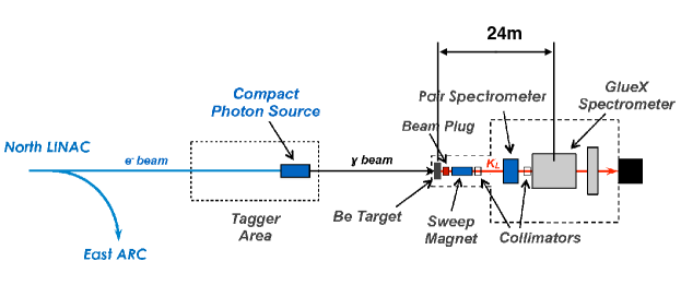
   Figure 1: Schematic view of Hall D beamline. See a text for explanation.

   Here we outline experimental conditions and simulated flux of $K_{L}^{0}$ based on GEANT4 and known cross sections of underlying subprocesses [5, 6, 7].

   The expected flux of $K_{L}^{0}$ mesons integrated in the range of momenta $P=0.3-10GeV/c$ will be on the order of $\sim 10^{4}$ $K_{L}^{0}/s$ on the physics target of the GlueX setup under the following conditions:

   • A thickness of the radiator 10$\%$.

   • The distance between Be and $LH_{2}$ targets in the range of 24 m.

   • The Be target with a length $L=40$ cm.

   In addition, the lower repetition rate of electron beam with 64 ns spacing between bunches will be required to have enough time to measure time-of-flight of the beam momenta and to avoid an overlap of events produced from alternating pulses. Low repetition rate was already successfully used by G0 experiment in Hall C at JLab [8].

   The final flux of $K_{L}^{0}$ is presented with 10$\%$ radiator, corresponding to maximal rate .

   In the production of a beam of neutral kaons, an important factor is the rate of neutrons as a background. As it is well known, the ratio $R=N_{n}/N_{K_{L}^{0}}$ is on the order $10^{3}$ from primary proton beams [9], the same ratio with primary electromagnetic interactions is much lower. This is illustrated in Fig. 2, which presents the rate of kaons and neutrons as a function of the momentum, which resembles similar behavior as it was measured at SLAC [10].

   

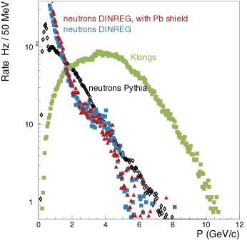
   Figure 2: The rate of neutrons (open symbols) and $K_{L}^{0}$ (full squares) on $LH_{2}$ target of Hall D as a function of their momenta simulated with different MC generators with $10^{4}K^{0}_{L}$/sec.

   Shielding of the low energy neutrons in the collimator cave and flux of neutrons has been estimated to be affordable, however detailed simulations are under way to show the level of radiation along the beamline.

   Th response of GlueX setup, reconstruction efficiency and resolution are presented in a talk by Taylor in Ref. [1].

3. Expected Rates

   In this section, we discuss expected rates of events for some selected reactions. The production of $\Xi$ hyperons has been measured only with charged kaons with very low statistical precision and never with primary $K_{L}^{0}$ beam. In Fig. 3, panel (a) shows existing data for the octet ground state $\Xi$’s with theoretical model predictions for $W$ (the reaction center of mass energy) distribution, panel (b) shows the same model prediction [11] presented with expected experimental points and statistical error for 10 days of running with our proposed setup with a beam intensity $2\times 10^{3}\leavevmode\nobreak\ K_{L}$/sec using missing mass of $K^{+}$ in the reaction $K_{L}^{0}+p\to K^{+}\Xi^{0}$ without detection of any of decay products of $\Xi^{0}$ (for more details on this topic see a talk by Nakayama in Ref. [1]).

   

   

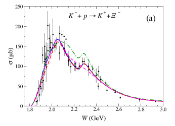
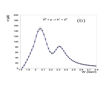
   Figure 3: (a) Cross section for existing world data on $K^{-}+p\to K^{+}\Xi^{-}$ reaction with model predictions from Ref. [11]; (b) expected statistical precision for the reaction $K_{L}^{0}+p\to K^{+}\Xi^{0}$ in 10 days of running with a beam intensity $2\times 10^{3}K_{L}$/sec overlaid on theoretical prediction [11].

   The physics of excited hyperons is not well explored, remaining essentially at the pioneering stages of ’70s-’80s. This is especially true for $\Xi^{\ast}(S=-2)$ and $\Omega^{\ast}(S=-3)$ hyperons. For example, the $SU(3)$ flavor symmetry allows as many $S=-2$ baryon resonances, as there are $N$ and $\Delta$ resonances combined ($\approx 27$); however, until now only three [ground state $\Xi(1382)1/2^{+}$, $\Xi(1538)3/2^{+}$, and $\Xi(1820)3/2^{-}$] have their quantum numbers assigned and few more states have been observed [12]. The status of $\Xi$ baryons is summarized in a table presented in Fig. 4 together with the quark model predicted states [13].

   

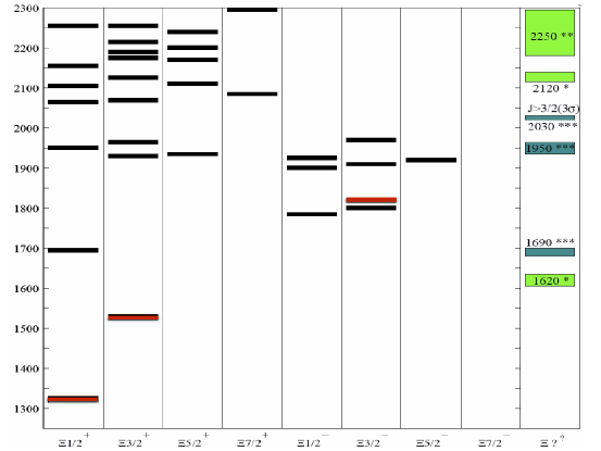
   Figure 4: Black bars: Predicted $\Xi$ spectrum based on the quark model calculation [13]. Colored bars: Observed states. The two ground octet and decuplet states together with $\Xi(1820)$ in the column $J^{P}=3/2^{-}$ are shown in red color. Other observed states with unidentified spin-parity are plotted in the rightest column.

   Historically the $\Xi^{\ast}$ states were intensively searched for mainly in bubble chamber experiments using the $K^{-}p$ reaction in ’60s-’70s. The cross section was estimated to be on the order of 1-10 $\mu b$ at the beam momenta up to  10 GeV/c. In ’80s-’90s, the mass or width of ground and some of excited states were measured with a spectrometer in the CERN hyperon beam experiment. Few experiments have studied cascade baryons with the missing mass technique. In 1983, the production of $\Xi^{\ast}$ resonances up to 2.5 GeV were reported from $p(K^{-},K^{+})$ reaction from the measurement of the missing mass of $K^{+}$ [14]. The experimental situation with $\Omega^{-\ast}$’s is even worse than the $\Xi^{\ast}$ case, there are very few data for excited states. The main reason for such a scarce dataset in multi strange hyperon domain is mainly due to very low cross section in indirect production with pion or in particular- photon beams. Currently only ground state $\Omega^{-}$ quantum numbers are identified. Recently significant progress is made in lattice QCD calculations of excited baryon states [15, 16] which poses a challenge to experiments to map out all predicted states (for more details see a talk by Richards at this workshop). The advantage of baryons containing one or more strange quarks for lattice calculations is that then number of open decay channels is in general smaller than for baryons comprising only the light u and d quarks. Moreover, lattice calculations show that there are many states with strong gluonic content in positive parity sector for all baryons. The reason why hybrid baryons have not attracted the same attention as hybrid mesons is mainly due to the fact that they lack manifest “exotic" character. Although it is difficult to distinguish hybrid baryon states, there is significant theoretical insight to be gained from studying spectra of excited baryons, particularly in a framework that can simultaneously calculate properties of hybrid mesons. Therefore this program will be very much complementary to the GlueX physics program of hybrid mesons.

   The proposed experiment with a beam intensity $10^{4}K_{L}$/sec will result in about $2\times 10^{5}$ $\Xi^{\ast}$’s and $4\times 10^{3}$ $\Omega^{\ast}$’s per month.

   A similar program for KN scattering is under development at J-PARC with charged kaon beams. The current maximum momentum of secondary beamline of 2 GeV/c is available at the K1.8 beamline. The beam momentum of 2 GeV/c corresponds to $\sqrt{s}$=2.2 GeV in the $K^{-}p$ reaction which is not enough to generate even the first excited $\Xi^{\ast}$ state predicted in the quark model. However, there are plans to create high energy beamline in the momentum range 5-15 GeV/c to be used with the spectrometer commonly used with the J-PARC P50 experiment which will lead to expected yield of $(3-4)\times 10^{5}$ $\Xi^{\ast}$’s and $10^{3}$ $\Omega^{\ast}$’s per month.

   Statistical power of proposed experiment with $K_{L}$ beam at JLab will be of the same order as that in J-PARC with charged kaon beam.

   An experimental program with kaon beams will be much richer and allows to perform a complete experiment using polarized target and measuring recoil polarization of hyperons. This studies are under way to find an optimal solution for the GlueX setup.

   The strange meson spectroscopy is another important subject for $K_{L}$ Facility at JLab. The high intensity $K_{L}$ beam will allow to study final state $K-\pi$ system. In particluar to perform phase shift analysis for different partial-waves, which may have significant imact to all systems having $K-\pi$ in the final state. This includes heavy $D$- and $B$-meson decays as well as $\tau\to K\pi\nu_{\tau}$ decay.

4. Summary

   In summary we intend to propose production of high intensity $K_{L}$ beam using photoproduction processes from a secondary Be target. A flux as high as $\sim 10^{4}K_{L}$/sec could be achieved. Momenta of $K_{L}$ beam particles will be measured with time-of-flight. The flux of kaon beam will be measured through partial detection of $\pi^{+}\pi^{-}$ decay products from their decay to $\pi^{+}\pi^{-}\pi^{0}$ by exploiting similar procedure used by LASS experiment at SLAC [10]. Besides using unpolarized liquid hydrogen target currently installed in GlueX experiment the unpolarized deuteron target may be installed. Additional studies are needed to find an optimal choice of polarized targets. This proposal will allow to measure $KN$ scattering with different final states including production of strange and multi strange baryons with unprecedented statistical precision to test QCD in non perturbative domain. It has a potential to distinguish between different quark models and test lattice QCD predictions for excited baryon states with strong hybrid content. It will also be used to study $\pi-K$ interactions, which is the topic of the current workshop.

5. Acknowledgments

   My research is supported by DOE Grant-100388-150.

3.2 Kaon-pion Scattering from Lattice QCD

Colin Morningstar

Carnegie Mellon University

Pittsburgh, PA 15213, U.S.A.

1. A key goal in lattice QCD is the determination of the spectrum of hadronic resonances from first principles. One of the best methods of computing the masses and other properties of hadrons from QCD involves estimating the QCD path integrals using Markov-chain Monte Carlo methods, which requires formulating the theory on a space-time lattice. Such calculations are necessarily carried out in finite volume. However, most of the excited hadrons we seek to study are unstable resonances. Fortunately, it is possible to deduce the masses and widths of resonances from the spectrum determined in finite volume. The method we use is described in Ref. [1] and the references contained therein.

   To study low-lying resonances in lattice QCD, we first use lattice QCD methods to calculate the interacting two-particle lab-frame energies $E$ in a spatial $L^{3}$ volume with periodic boundary conditions. Our stationary states have total momentum $\bm{P}=(2\pi/L)\bm{d}$, where $\bm{d}$ is a vector of integers. We boost the lab-frame energies to the center-of-momentum frame using

   $$E_{\rm cm}=\sqrt{E^{2}-\bm{P}^{2}},\qquad\gamma=\frac{E}{E_{\rm cm}}.$$ (1)

   Assuming there are $N_{d}$ channels with particle masses $m_{1a},m_{2a}$ and spins $s_{1a},s_{2a}$ of particle 1 and 2 for each decay channel, we can define

   $$\bm{q}_{{\rm cm},a}^{2} = \frac{1}{4}E_{\rm cm}^{2}-\frac{1}{2}(m_{1a}^{2}+m_{2a}^{2})+\frac{(m_{1a}^{2}-m_{2a}^{2})^{2}}{4E_{\rm cm}^{2}},$$ (2)

   $$u_{a}^{2} = \frac{L^{2}\bm{q}_{{\rm cm},a}^{2}}{(2\pi)^{2}},\qquad\bm{s}_{a}=\left(1+\frac{(m_{1a}^{2}-m_{2a}^{2})}{E_{\rm cm}^{2}}\right).$$ (3)

   The relationship between the finite-volume energies $E$ and the scattering matrix$S$ is given by

   $$\det[1+F^{(\bm{P})}(S-1)]=0,$$ (4)

   where the $F$-matrix in the $JLSa$ basis states is given by

   $$\langle J^{\prime}m_{J^{\prime}}L^{\prime}S^{\prime}a^{\prime}|F^{(\bm{P})}|Jm_{J}LSa\rangle=\delta_{a^{\prime}a}\delta_{S^{\prime}S}\ \frac{1}{2}\Bigl{\{}\delta_{J^{\prime}J}\delta_{m_{J^{\prime}}m_{J}}\delta_{L^{\prime}L}$$

   $$\qquad+\langle J^{\prime}m_{J^{\prime}}|L^{\prime}m_{L^{\prime}}Sm_{S}\rangle\langle Lm_{L}Sm_{S}|Jm_{J}\rangle W_{L^{\prime}m_{L^{\prime}};\ Lm_{L}}^{(\bm{P}a)}\Bigr{\}},$$ (5)

   and where $J,J^{\prime}$ indicate total angular momenta, $L,L^{\prime}$ are orbital angular momenta, $S,S^{\prime}$ are intrinsic spins, and $a,a^{\prime}$ denote all other identifying information, such as decay channel. The $W$-matrix is given by

   $$-iW^{(\bm{P}a)}_{L^{\prime}m_{L^{\prime}};\ Lm_{L}}=\sum_{l=|L^{\prime}-L|}^{L^{\prime}+L}\sum_{m=-l}^{l}\frac{{\cal Z}_{lm}(\bm{s}_{a},\gamma,u_{a}^{2})}{\pi^{3/2}\gamma u_{a}^{l+1}}\sqrt{\frac{(2{L^{\prime}}+1)(2l+1)}{(2L+1)}}$$

   $$\qquad\qquad\times\langle{L^{\prime}}0,l0|L0\rangle\langle{L^{\prime}}m_{L^{\prime}},lm|Lm_{L}\rangle,$$ (6)

   and the Rummukainen-Gottlieb-Lüscher (RGL) shifted zeta functions ${\cal Z}_{lm}$ are evaluated using

   $${\cal Z}_{lm}(\bm{s},\gamma,u^{2})=\sum_{\bm{n}\in\mathbb{Z}^{3}}\frac{{\cal Y}_{lm}(\bm{z})}{(\bm{z}^{2}-u^{2})}e^{-\Lambda(\bm{z}^{2}-u^{2})}+\delta_{l0}\frac{\gamma\pi}{\sqrt{\Lambda}}F_{0}(\Lambda u^{2})$$

   $$+\frac{i^{l}\gamma}{\Lambda^{l+1/2}}\int_{0}^{1}\!\!dt\left(\frac{\pi}{t}\right)^{l+3/2}\!e^{\Lambda tu^{2}}\sum_{\bm{n}\in\mathbb{Z}^{3}\atop\bm{n}\neq 0}e^{\pi i\bm{n}\cdot\bm{s}}{\cal Y}_{lm}(\mathbf{w})\ e^{-\pi^{2}\mathbf{w}^{2}/(t\Lambda)}$$ (7)

   where

   $$\bm{z}=\bm{n}-\gamma^{-1}\bigl{[}\textstyle\frac{1}{2}+(\gamma-1)s^{-2}\bm{n}\cdot\bm{s}\bigl{]}\bm{s},$$ (8)

   $$\mathbf{w}=\bm{n}-(1-\gamma)s^{-2}\bm{s}\cdot\bm{n}\bm{s},\qquad{\cal Y}_{lm}(\mathbf{x})=|\mathbf{x}|^{l}\ Y_{lm}(\widehat{\mathbf{x}})$$ (9)

   $$F_{0}(x)=-1+\frac{1}{2}\int_{0}^{1}\!\!dt\ \frac{e^{tx}-1}{t^{3/2}}.$$ (10)

   We choose $\Lambda\approx 1$ for fast convergence of the summation, and the integral in Eq. (7) is done using Gauss-Legendre quadrature. $F_{0}(x)$ given in terms of the Dawson or erf function.

   The quantization condition in Eq. (4) relates a single energy $E$ to the entire $S$-matrix. This equation cannot be solved for $S$, except in the case of a single channel and single partial wave. To proceed, we approximate the $S$-matrix using functions depending on a handful of fit parameters, then obtain estimates of these parameters using fits involving as many energies as possible. It is easier to parametrize a Hermitian matrix than a unitary matrix, so we use the $K$-matrix defined as usual by

   $$S=(1+iK)(1-iK)^{-1}=(1-iK)^{-1}(1+iK).$$ (11)

   The Hermiticity of the $K$-matrix ensures the unitarity of the $S$-matrix. With time reversal invariance, the $K$-matrix must be real and symmetric. The multichannel effective range expansion suggests writing

   $$K^{-1}_{L^{\prime}S^{\prime}a^{\prime};\ LSa}(E)=u_{a^{\prime}}^{-L^{\prime}-\frac{1}{2}}\ {\widetilde{K}}^{-1}_{L^{\prime}S^{\prime}a^{\prime};\ LSa}(E_{\rm cm})\ u_{a}^{-L-\frac{1}{2}}$$ (12)

   since ${\widetilde{K}}^{-1}_{L^{\prime}S^{\prime}a^{\prime};\ LSa}(E_{\rm cm})$ should behave smoothly with $E_{\rm cm}$, then the quantization condition can be written

   $$\det(1-B^{(\bm{P})}\widetilde{K})=\det(1-\widetilde{K}B^{(\bm{P})})=0,$$ (13)

   where we define the important box matrix by

   $$\langle J^{\prime}m_{J^{\prime}}L^{\prime}S^{\prime}a^{\prime}|\ B^{(\bm{P})}\ |Jm_{J}LSa\rangle=-i\delta_{a^{\prime}a}\delta_{S^{\prime}S}\ u_{a}^{L^{\prime}+L+1}\ W_{L^{\prime}m_{L^{\prime}};\ Lm_{L}}^{(\bm{P}a)}$$

   $$\qquad\qquad\times\langle J^{\prime}m_{J^{\prime}}|L^{\prime}m_{L^{\prime}},Sm_{S}\rangle\langle Lm_{L},Sm_{S}|Jm_{J}\rangle.$$ (14)

   The box matrix is Hermitian for $u_{a}^{2}$ real. The quantization condition can also be expressed as

   $$\det(\widetilde{K}^{-1}-B^{(\bm{P})})=0,$$ (15)

   and the determinants in Eqs. (13) and (15) are real.

   The quantization condition involves a determinant of an infinite matrix. To make such determinants practical for use, we first transform to a block-diagonal basis, and then truncate in orbital angular momentum. For a symmetry operation $G$, define theunitary matrix

   $$\langle J^{\prime}m_{J^{\prime}}L^{\prime}S^{\prime}a^{\prime}|\ Q^{(G)}\ |Jm_{J}LSa\rangle=\left\{\begin{array}[]{ll}\delta_{J^{\prime}J}\delta_{L^{\prime}L}\delta_{S^{\prime}S}\delta_{a^{\prime}a}D^{(J)}_{m_{J^{\prime}}m_{J}}(R),&(G=R),\\ \delta_{J^{\prime}J}\delta_{m_{J^{\prime}}m_{J}}\delta_{L^{\prime}L}\delta_{S^{\prime}S}\delta_{a^{\prime}a}(-1)^{L},&(G=I_{s}),\end{array}\right.$$ (16)

   where $D^{(J)}_{m^{\prime}m}(R)$ are the Wigner rotation matrices, $R$ is an ordinary rotation, and $I_{s}$ is spatial inversion. One can show that the box matrix satisfies

   $$B^{(G\bm{P})}=Q^{(G)}\ B^{(\bm{P})}\ Q^{(G)\dagger}.$$ (17)

   If $G$ is in the little group of $\bm{P}$, then $G\bm{P}=\bm{P},\ G\bm{s}_{a}=\bm{s}_{a}$ and

   $$[B^{(\bm{P})},Q^{(G)}]=0,\qquad\mbox{($G$ in little group of $\bm{P}$).}$$ (18)

   This means we can use the eigenvectors of $Q^{(G)}$ to block diagonalize $B^{(\bm{P})}$. The block-diagonal basis can be expressed using

   $$\left|\Lambda\lambda nJLSa\right\rangle=\sum_{m_{J}}c^{J(-1)^{L};\,\Lambda\lambda n}_{m_{J}}\left|Jm_{J}LSa\right\rangle$$ (19)

   for little group irrep $\Lambda$, irrep row $\lambda$, and occurrence index $n$. The transformation coefficients depend on $J$ and $(-1)^{L}$, but not on $S,a$. Essentially, the transformation replaces $m_{J}$ by $(\Lambda,\lambda,n)$. Group theoretical projections with Gram-Schmidt are used to obtain the basis expansion coefficients. In this block-diagonal basis, the box matrix has the form

   $$\langle\Lambda^{\prime}\lambda^{\prime}n^{\prime}J^{\prime}L^{\prime}S^{\prime}a^{\prime}|\ B^{(\bm{P})}\ |\Lambda\lambda nJLSa\rangle=\delta_{\Lambda^{\prime}\Lambda}\delta_{\lambda^{\prime}\lambda}\delta_{S^{\prime}S}\delta_{a^{\prime}a}\ B^{(\bm{P}\Lambda_{B}Sa)}_{J^{\prime}L^{\prime}n^{\prime};\ JLn}(E_{\rm cm}),$$ (20)

   and the $\widetilde{K}$-matrix for $(-1)^{L+L^{\prime}}=1$ has the form

   $$\langle\Lambda^{\prime}\lambda^{\prime}n^{\prime}J^{\prime}L^{\prime}S^{\prime}a^{\prime}|\ \widetilde{K}\ |\Lambda\lambda nJLSa\rangle=\delta_{\Lambda^{\prime}\Lambda}\delta_{\lambda^{\prime}\lambda}\delta_{n^{\prime}n}\delta_{J^{\prime}J}\ {\cal K}^{(J)}_{L^{\prime}S^{\prime}a^{\prime};\ LSa}(E_{\rm cm}).$$ (21)

   $\Lambda$ is the irrep for the $K$-matrix, but we need $\Lambda_{B}$ for the box matrix. When $\eta^{P}_{1a}\eta^{P}_{2a}=1$, then $\Lambda_{B}=\Lambda$, but they differ slightly when $\eta^{P}_{1a}\eta^{P}_{2a}=-1$.

   

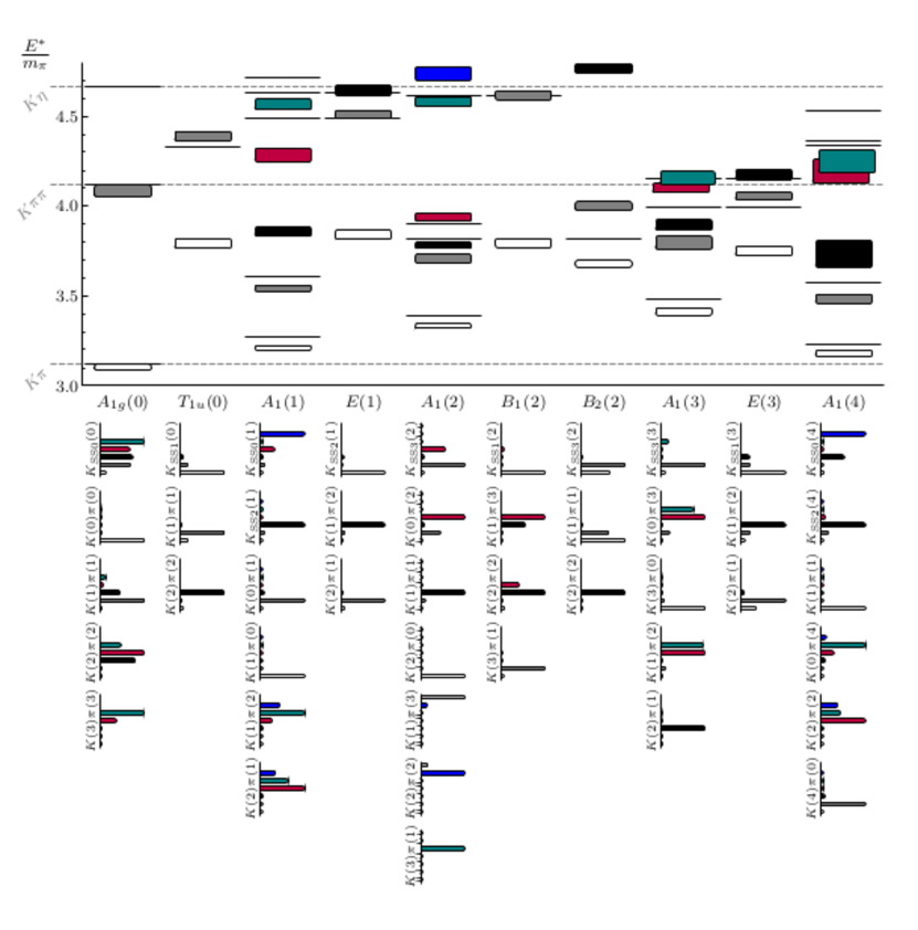
   Figure 1: Center-of-momentum energies over the pion mass in the isodoublet strange mesonic sector for a $32^{3}\times 256$ anisotropic lattice with $m_{\pi}\sim 240$ MeV. Each irrep is located in one column, where the energy ratios are shown in the upper panel with a vertical thickness showing the statistical error. The solid horizontal lines should the two-hadron noninteracting energies, and the gray dashed lines show relevant thresholds. The corresponding columns in the lower panel indicate overlaps of each interpolating operator onto the finite-volume Hamiltonian eigenstates.

   Table 1: Best-fit results for various parameters related to the $K^{\ast}(892)$ calculations.

   Fit	$s$-wave par.	$m_{K^{\ast}}/m_{\pi}$	$g_{K^{\ast}K\pi}$	$m_{\pi}a_{0}$	$\chi^{2}/\mathrm{d.o.f.}$
   (1a,1b)	lin	$3.819(20)$	$5.54(25)$	$-0.333(31)$	($1.04,$–)
   2	lin	$3.810(18)$	$5.30(19)$	$-0.349(25)$	$1.49$
   3	quad	$3.810(18)$	$5.31(19)$	$-0.350(25)$	$1.47$
   4	ere	$3.809(17)$	$5.31(20)$	$-0.351(24)$	$1.47$
   5	bw	$3.808(18)$	$5.33(20)$	$-0.353(25)$	$1.42$
   6	bw	$3.810(17)$	$5.33(20)$	$-0.354(25)$	$1.50$

   Using a large set of single- and two-hadron operators, as described in Ref. [2], for several different total momenta, we have evaluated a large number of energies in the isodoublet $I=\frac{1}{2}$ strange $S=1$ mesonic sector [3]. We used an anisotropic $32^{3}\times 256$ lattice with a pion mass $m_{\pi}\sim 240$ MeV. The determinations of these energies are possible since we use the stochastic LapH method [4] to estimate all quark propagation. The center-of-momentum energies over the pion mass are shown in Fig. 1. Horizontal lines indicates the non-interacting two-hadron energies, and the dashed lines show the $K\pi$, $K\pi\pi$, and $K\eta$ thresholds. Operator overlaps are shown in the lower panel of the figure.

   To extract the resonance properties of the $K^{\ast}(892)$, we included the $L=0,1,2$ partial waves. The fit forms used for the $P$ and $D$ partial waves were

   $$(\widetilde{K}^{-1})_{11} = \frac{6\pi E_{\rm cm}}{g_{K^{\ast}\pi\pi}^{2}m_{\pi}}\left(\frac{m_{K^{\ast}}^{2}}{m_{\pi}^{2}}-\frac{E_{\rm cm}^{2}}{m_{\pi}^{2}}\right),\qquad(\widetilde{K}^{-1})_{22}=\frac{-1}{m_{\pi}^{5}a_{2}},$$ (22)

   and for the $S$-wave, several different forms were tried:

   $$(\widetilde{K}^{-1})_{00}^{\rm lin} = a_{\rm l}+b_{\rm l}E_{\rm cm},$$ (23)

   $$(\widetilde{K}^{-1})_{00}^{\rm quad} = a_{\rm q}+b_{\rm q}E_{\rm cm}^{2},$$ (24)

   $$(\tilde{K}^{-1})_{00}^{\textsc{ERE}} = \frac{-1}{m_{\pi}a_{0}}+\frac{m_{\pi}r_{0}}{2}\frac{q^{2}_{{\mathrm{cm}}}}{m_{\pi}^{2}},$$ (25)

   $$(\tilde{K}^{-1})_{00}^{\textsc{bw}} = \left(\frac{m^{2}_{K_{0}^{\ast}}}{m^{2}_{\pi}}-\frac{E^{2}_{{\mathrm{cm}}}}{m_{\pi}^{2}}\right)\frac{6\pi m_{\pi}E_{{\mathrm{cm}}}}{g_{K_{0}^{\ast}\pi\pi}^{2}m^{2}_{K_{0}^{\ast}}}.$$ (26)

   A summary of our fit results is presented in Table 1. Our determinations of the partial-wave scattering phase shifts are shown in Fig. 2. We found that the $q\overline{q}$ operators in the $A_{1g}(0)$ channel overlap many of the eigenvectors in this channel. Better energy resolution is needed for a determination of the $K_{0}^{\ast}(800)$ parameters, which will be done in the future, but an NLO effective range parametrization finds $m_{R}/m_{\pi}=4.66(13)-0.87(18)i$, consistent with a Breit-Wigner fit. In Ref. [3], our results are compared to the few other recent lattice results [5, 6, 7] that are available. See also Ref. [8].

   We have also recently determined the decay width of the $\rho$-meson, including $L=1,3,5$ partial waves [9], as well as the $\Delta$ baryon [10].

   

   

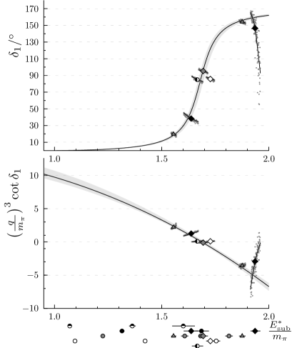
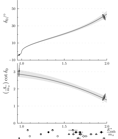
   Figure 2: (Left) Our determination of the $P$-wave $I=\frac{1}{2}$ $K\pi$ scattering phase shift $\delta_{1}$ and $q_{{\mathrm{cm}}}^{3}\cot\delta_{1}$ using a $32^{3}\times 256$ anisotropic lattice with $m_{\pi}\sim 240$ MeV. (Right) Our calculations of the $S$-wave scattering phase shift $\delta_{0}$ (quadratic fit) and $q_{{\mathrm{cm}}}\cot\delta_{0}$. Results are from Ref. [3].

2. Acknowledgments

   This work was done in collaboration with John Bulava (U. Southern Denmark), Ruairi Brett (CMU), Daniel Darvish (CMU), Jake Fallica (U. Kentucky), Andrew Hanlon (U. Mainz), Ben Hoerz (U. Mainz), and Christian W Andersen (U. Southern Denmark). I thank the organizers, especially Igor Strakovsky, and JLab for the opportunity to participate in this Workshop. This work was supported by the U.S. National Science Foundation under award PHY–1613449. Computing resources were provided by the Extreme Science and Engineering Discovery Environment (XSEDE) under grant number TG-MCA07S017. XSEDE is supported by National Science Foundation grant number ACI-1548562.

3.3 K-$\pi$ Scattering with $K_{L}$ Beam Facility

Marouen Baalouch

Department of Physics

Old Dominion University

Norfolk, VA 23529, U.S.A. &

Thomas Jefferson National Accelerator Facility

Newport News, VA 23606, U.S.A.

1. Introduction

   The $K_{L}$ Beam Facility can offer a good opportunity to study the kaon-pion interaction experimentally, by producing the final state $K\pi$ using the scattering of a neutral kaon off proton or neutron as $K_{L}N\rightarrow[K\pi]N^{\prime}$. The analysis of the kaon-pion interaction experimentally has several implication on the imperfect phenomenological studies, as the test of the Chiral Perturbation Theory, Strange Meson Spectroscopy and Physics beyond Standard Model. These phenomenological studies require more data to improve the precision on the observable of interest. So far, the main experimental data used to study kaon-pion scattering at low energy comes from kaon beam experiments at SLAC in the 1970s and 1980s.

2. Chiral Perturbation Theory

   In Quantum Chromodynamics (QCD), the strong interaction coupling constant increases with decreasing energy. This means that the coupling becomes large at low energies, and one can no longer rely on perturbation theory. Few phenomenological approaches can be used at this energy level, as Lattice QCD or the Chiral Perturbation Theory (ChPT) [1]. The purpose of the ChPT is to use an effective Lagrangian where the mesons $\pi$, $\eta$, and $K$, called also Goldstone Bosons, are the fundamental degrees of freedom. The ChPT studies on on the $\pi\pi$ scattering amplitude shows a good agreement with the experimental studies ($e.g.$, see reference [2]). However, this theory is less successful with the $K\pi$ scattering amplitude [3, 4, 5, 6, 7, 8, 9], and so far no accurate experimental data is available at low energy.

3. Strange Meson Spectroscopy

   Hadron Spectroscopy plays an important role to understand QCD in the non perturbative domain by performing a quantitative understanding of quark and gluon confinement, and validate Lattice QCD prediction. In the last years, an important number of resonances have been identified, especially resonances with heavy flavored quark. However, the sector of strange baryons and mesons was not significantly improved and several estimated states by lattice QCD and quark model still not yet observed. Moreover, the identification of the scalar strange light mesons, as $\kappa$ and $K^{\ast}_{0}(1430)$, still a long-standing puzzle because of their large decay width that causes an overlap between resonances at low Lorentz-invariant mass. The indications on the presence of $\kappa$ resonance have been reported based on the data of the E791 [10] and BES [11] Collaborations and several phenomenological studies [12, 13, 14] have been made to measure the pole of $\kappa$ resonance. However, the results from Roy-Steiner dispersive representation [12] not in good agreement with low energy experimental data, and the confirmation of this pole in the amplitude for elastic $K\pi$ scattering requires more data at low energy. The $K^{\ast}_{0}(1430)$ is the second scalar strange resonance which is also not well understood. And recently the $K\pi$ $S$-wave amplitude extracted from $\eta_{c}\to KK\pi$ [15] found to be very different with respect to the amplitude measured by LASS and E791. Fig 1, taken from the reference [15], shows the comparison of the amplitude extracted from $\eta_{c}\to KK\pi$, $Kp\to K\pi n$ and $D\to KK\pi$.

   The light strange scalar mesons can be produced in $KN$ scattering, and more data from these type of reactions will certainly improve the understanding of the non well identified strange resonances.

   

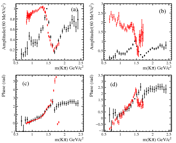
   Figure 1: Figure taken from ref  [15]: The I=1/2 $K\pi$ S-wave amplitude measurements from $\eta_{c}\to KK\pi$ compared to the (a) LASS and (b) E791 results: the corresponding I=1/2 $K\pi$ S-wave phase measurements compared to the (c) LASS and (d) E791 measurements. Black dots indicate the results from the present analysis; square (red) points indicate the LASS or E791 results. The LASS data are plotted in the region having only one solution.

4. $K\pi$ Scattering Amplitude and Physics Beyond Standard Model

   The determination of the CKM matrix elements $V_{us}$ is mainly performed using $\tau$ or kaon decays. As an example, the $V_{us}$ matrix element is accessible from the $K_{l3}$ decays using the braching ratio function

   $$\Gamma(K\to\pi l\nu)\propto N|V_{us}|^{2}|f^{K\pi}_{+}(0)|^{2}I_{K}^{l},$$ (1)

   where

   $$I_{K}=\int{\rm d}t\frac{1}{m_{K}^{8}}\lambda^{3/2}F(\widetilde{f}_{+}(t),\widetilde{f}_{0}(t)).$$ (2)

   In this function $f^{K\pi}_{0}$ and $f^{K\pi}_{+}$ represent the form factors of the strangeness changing scalar and vector, respectively. These form factors in the low energy region, can be obtained from Lattice QCD or from the study of the $K\pi$ scattering using dispersion relation analysis [16]. The precision on $V_{us}$ depends strongly on the precision of these strangeness changing form factors. And by improving the precision of $V_{us}$ one can probe the physics beyond the standard model indirectly thanks to the unitarity of the CKM matrix

   $$|V_{ud}|^{2}+|V_{us}|^{2}+|V_{ub}|^{2}=1.$$ (3)

   Therefore, any shift from unitarity is a sign of physics beyond Standard Model. Fig 2 shows the fit to the different CKM elements involved in the unitarity equation.

   

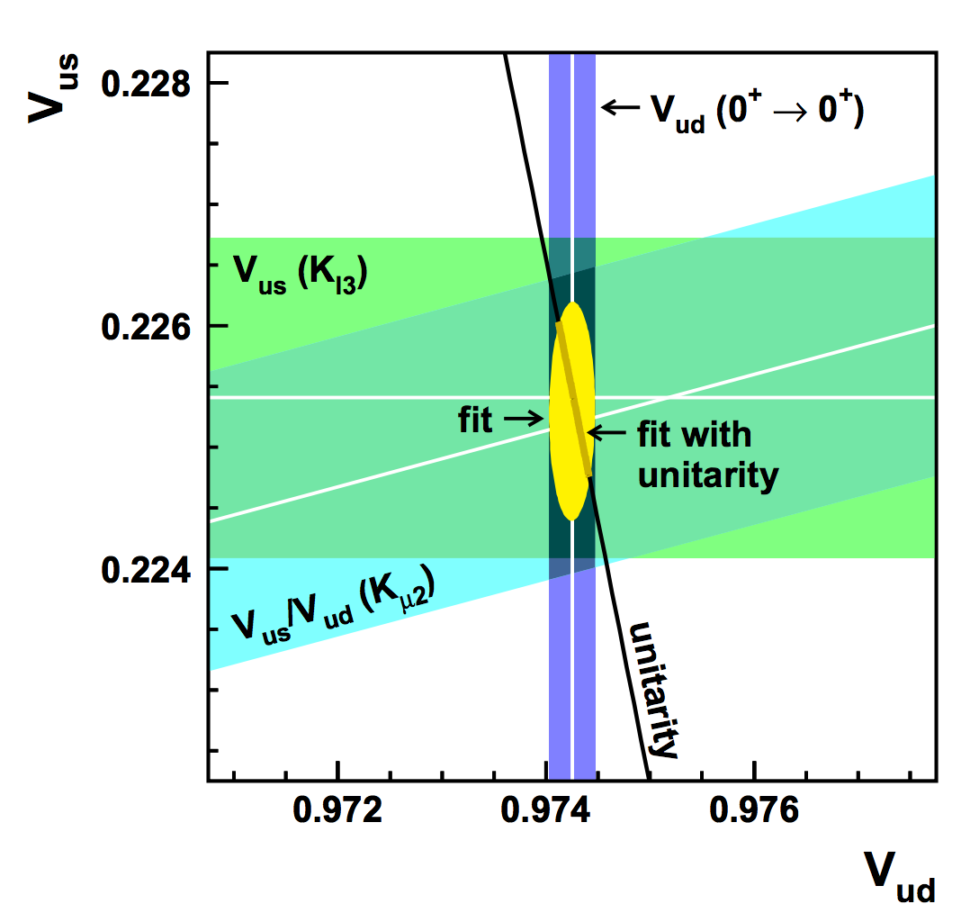
   Figure 2: Figure taken from Ref. [17]: Results of fits to $|V_{us}|$, $|V_{us}|$, and $|V_{ud}/V_{us}|$.

5. Kaon-Production and GlueX Detector

   The hadroproduction of the $K\pi$ system has been intensively studied with charged Kaon beam [18, 19, 20, 21, 22]. However, few studies have been made using a neutral kaon beam. The production mechanism of the $K\pi$ system with charged kaon beam is proportional to the mechanism with neutral kaon, the main difference related to the Clebsch-Gordan coefficients. In LASS analysis [18], the $K\pi$ production mechanism is parametrized using a model consisting of exchange degenerate Regge poles together with non-evasive “cut" contributions. These parameterization was extrapolated to the neutral kaon beam and used in the simulation of $K_{\rm L}p\to[K\pi]^{0}p$ in KLF where the reconstruction of the events is made by GlueX spectrometer. The GlueX spectrometer is built in Hall D at JLab and using photon beam scattering off proton to provide critical data needed to address one of the outstanding and fundamental challenges in physics the quantitative understanding of the confinement of quarks and gluons in QCD. The GlueX detector is azimuthally symmetric and nearly hermetic for both charged particles and photons, which make it a relevant detector for studying $K\pi$ scattering amplitude. Fig 3 shows the kinematics region that can be covered by the detector using the simulation of $K_{\rm L}p\to[K\pi]^{0}p$ and LASS parameterization. More details about the detector performance can be found in reference [23].

   

   

   

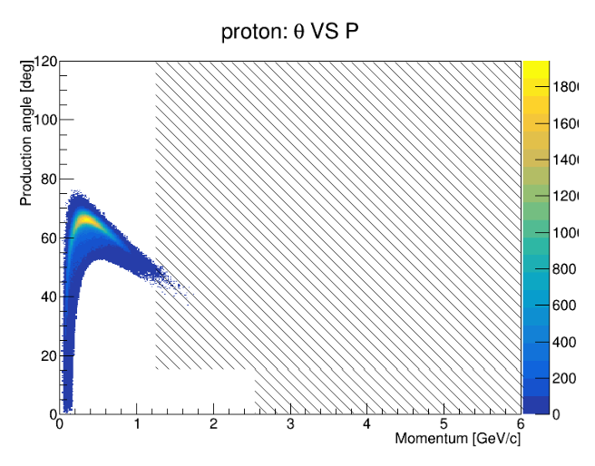
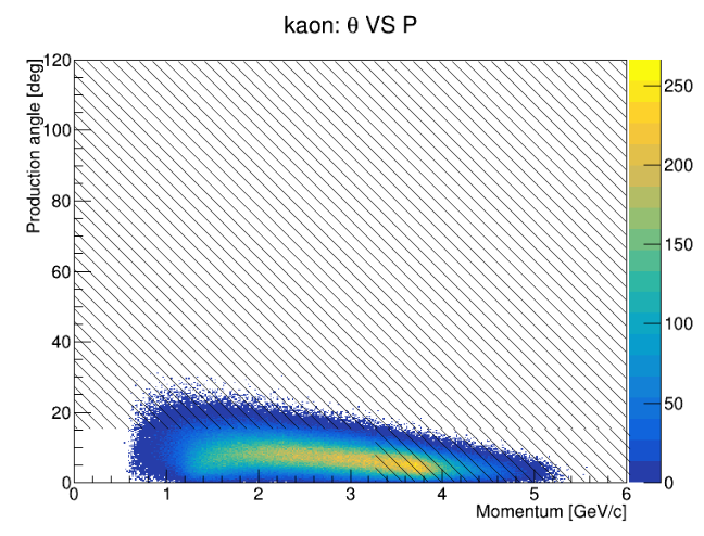
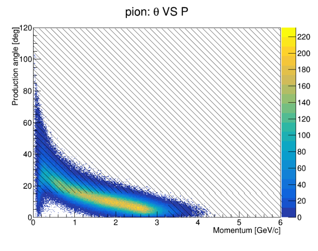
   Figure 3: The simulated events of the reaction $K_{\rm L}p\to[K\pi]^{0}p$ projected on the plane of the production angle (in the Lab frame) $\theta$ versus the magnitude of the momentum. The dashed region represents the region where the GlueX detector performance of Particle Identification are low: on the top left for the proton, on the top right for the kaon and on the bottom for the pion.

6. Acknowledgments

   My research is supported by Old Dominion University, Old Dominion University Research Foundation and Jefferson Laboratory.

3.4 Dalitz Plot Analysis of Three-body Charmonium Decays at BaBar

Antimo Palano (on behalf of the BaBar Collaboration)

I.N.F.N. and University of Bari

Bari 70125, Italy

1. Introduction

   Charmonium decays can be used to obtain new information on light meson spectroscopy. In $e^{+}e^{-}$ interactions, samples of charmonium resonances can be obtained using different processes.

   • In two-photon interactions we select events in which the $e^{+}$ and $e^{-}$ beam particles are scattered at small angles and remain undetected. Only resonances with $J^{PC}=0^{\pm+},2^{\pm+},3^{++},4^{\pm+}$…. can be produced.

   • In the Initial State Radiation (ISR) process, we reconstruct events having a (mostly undetected) fast forward $\gamma_{ISR}$ and, in this case, only $J^{PC}=1^{--}$ states can be produced.

2. Selection of Two-Photon Production of $\eta_{c}\to K^{+}K^{-}\eta$, $\eta_{c}\to K^{+}K^{-}\pi^{0}$, and $\eta_{c}\to K_{S}^{0}K^{\pm}\pi^{\mp}$

   We study the reactions

   $\gamma\gamma\to K^{+}K^{-}\eta$,      $\gamma\gamma\to K^{+}K^{-}\pi^{0}$,      $\gamma\gamma\to K_{S}^{0}K^{\pm}\pi^{\mp}$ ,

   where $\eta\to\gamma\gamma$ and $\eta\to\pi^{+}\pi^{-}\pi^{0}$ [1, 2].

   

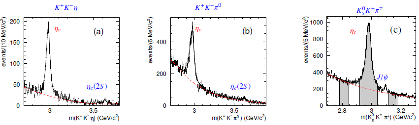
   Figure 1: (a) $K^{+}K^{+}\eta$, (b) $K^{+}K^{-}\pi^{0}$, and (c) $K_{S}^{0}K^{\pm}\pi^{\mp}$ mass spectra. The superimposed curves are from the fit results. In (c) the shaded area evidences definition of the signal and sidebands regions.

   Two-photon candidates are reconstructed from the sample of events having the exact number of charged tracks for that $\eta_{c}$ decay mode. Since two-photon events balance the transverse momentum, we require $p_{T}$, the transverse momentum of the system with respect to the beam axis, to be $p_{T}<0.05\leavevmode\nobreak\ GeV/c$ for $\eta_{c}\to K^{+}K^{-}\eta/\pi^{0}$ and $p_{T}<0.08\leavevmode\nobreak\ GeV/c$ for $\eta_{c}\to K_{S}^{0}K^{\pm}\pi^{\mp}$. We also define $M_{rec}^{2}\equiv(p_{e+e-}-p_{rec})^{2}$, where $p_{e+e-}$ is the four-momentum of the initial state and $p_{\mathrm{rec}}$ is the four-momentum of the three-hadrons system and remove ISR events requiring $M_{rec}^{2}>10\leavevmode\nobreak\ GeV^{2}/c^{4}$. Figure 1 shows the $K^{+}K^{-}\eta$, $K^{+}K^{-}\pi^{0}$, and $K_{S}^{0}K^{\pm}\pi^{\mp}$ mass spectra where signals of $\eta_{c}$ can be observed.

   Selecting events in the $\eta_{c}$ mass region, the Dalitz plots for the three $\eta_{c}$ decay modes are shown in Fig. 2. The $\eta_{c}\to K\bar{K}\pi$ Dalitz plots are dominated by the presence of horizontal and vertical uniform bands at the position of the $K_{0}^{\ast}(1430)$ resonance.

   

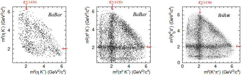
   Figure 2: (Left) $K^{+}K^{+}\eta$, (Center) $K^{+}K^{-}\pi^{0}$, and (Right) $K_{S}^{0}K^{\pm}\pi^{\mp}$ Dalitz plots. The arrows indicate the positions of the $K^{\ast}_{0}(1430)$ resonance.

   The $\eta_{c}$ signal regions contain 1161 events with (76.1$\pm$1.3)% purity for $\eta_{c}\to K^{+}K^{-}\eta$, 6494 events with (55.2$\pm$0.6)% purity for $\eta_{c}\to K^{+}K^{-}\pi^{0}$, and 12849 events with (64.3 $\pm$ 0.4)% purity for $\eta_{c}\to K_{S}^{0}K^{\pm}\pi^{\mp}$. The backgrounds below the $\eta_{c}$ signals are estimated from the sidebands. We observe asymmetric $K^{\ast}$’s in the background to the $\eta_{c}\to K_{S}^{0}K^{\pm}\pi^{\mp}$ final state due to interference between I=1 and I=0 contributions.

3. Dalitz Plot Analysis of $\eta_{c}\to K^{+}K^{-}\eta$ and $\eta_{c}\to K^{+}K^{-}\pi^{0}$

   We first perform unbinned maximum likelihood fits using the Isobar model [3]. Figure 3 shows the $\eta_{c}\to K^{+}K^{-}\eta$ Dalitz plot projections.

   

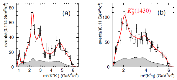
   Figure 3: $\eta_{c}\to K^{+}K^{-}\eta$ Dalitz plot analysis. (a) $K^{+}K^{-}$, and (b) $K^{\pm}\eta$ squared mass projections. Shaded is the background contribution.

   The analysis of the $\eta_{c}\to K^{+}K^{-}\eta$ decay requires significant contributions from $f_{0}(1500)\eta$ $(23.7\pm 7.0\pm 1.8)$% and $K^{\ast}_{0}(1430)^{+}K^{-}$ $(16.4\pm 4.2\pm 1.0)$%, where $K^{\ast}_{0}(1430)^{+}\to K^{+}\eta$: a first observation of this decay mode. It is found that the $\eta_{c}$ three-body hadronic decays proceed almost entirely through the intermediate production of scalar meson resonances. A similar analysis performed on the $\eta_{c}\to K^{+}K^{-}\pi^{0}$ allows to obtain the corresponding contribution from $K^{\ast}_{0}(1430)^{+}K^{-}$ to be $(33.8\pm 1.9\pm 0.4)$%, where $K^{\ast}_{0}(1430)^{+}\to K^{+}\pi^{0}$. Combining the above information with the measurement of the $\eta_{c}$ relative branching fraction

   $$\frac{BR(\eta_{c}\to K^{+}K^{-}\eta)}{BR(\eta_{c}\to K^{+}K^{-}\pi^{0})}=0.571\pm 0.025\pm 0.051,$$ (1)

   we obtain

   $$\frac{BR(K^{\ast}_{0}(1430)\to\eta K)}{BR(K^{\ast}_{0}(1430)\to\pi K)}=0.092\pm 0.025^{+0.010}_{-0.025}.$$ (2)

   We perform a Likelihood scan and obtain a measurement of the $K^{\ast}_{0}(1430)$ parameters

   $$m(K^{\ast}_{0}(1430))=1438\pm 8\pm 4\leavevmode\nobreak\ MeV/c^{2},\leavevmode\nobreak\ \leavevmode\nobreak\ \leavevmode\nobreak\ \leavevmode\nobreak\ \leavevmode\nobreak\ \leavevmode\nobreak\ \leavevmode\nobreak\ \Gamma(K^{\ast}_{0}(1430))=210\pm 20\pm 12\leavevmode\nobreak\ MeV.$$ (3)

4. Model Independent Partial Wave Analysis of $\eta_{c}\to K^{+}K^{-}\pi^{0}$ and $\eta_{c}\to K_{S}^{0}K^{\pm}\pi^{\mp}$

   We perform a Model Independent Partial Wave Analysis (MIPWA) [4] of $\eta_{c}\to K^{+}K^{-}\pi^{0}$ and $\eta_{c}\to K_{S}^{0}K^{\pm}\pi^{\mp}$. In the MIPWA the $K\pi$ mass spectrum is divided into 30 equally spaced mass intervals 60 MeV/c² wide and for each bin we add to the fit two new free parameters, the amplitude and the phase of the $K\pi$ $\mathcal{S}$-wave (constant inside the bin).

   We also fix the amplitude to 1.0 and its phase to $\pi/2$ in an arbitrary interval of the mass spectrum (bin 11 which corresponds to a mass of 1.45 GeV/c²). The number of additional free parameters is therefore 58. Due to isospin conservation in the decays, amplitudes are symmetrized with respect to the two $K\pi$ decay modes. The $K^{\ast}_{2}(1420)$, $a_{0}(980)$, $a_{0}(1400)$, $a_{2}(1310)$, … contributions are modeled as relativistic Breit-Wigner functions multiplied by the corresponding angular functions. Backgrounds are fitted separately and interpolated into the $\eta_{c}$ signal regions. The fits improves when an additional high mass $a_{0}(1950)\to K\bar{K}$, I=1 resonance, is included with free parameters in both $\eta_{c}$ decay modes. The weighted average of the two measurement is: $m(a_{0}(1950))=1931\pm 14\pm 22$ MeV/c², $\Gamma(a_{0}(1950))=271\pm 22\pm 29$ MeV. The statistical significances for the $a_{0}(1950)$ effect (including systematics) are $2.5\sigma$ for $\eta_{c}\to K_{S}^{0}K^{\pm}\pi^{\mp}$ and $4.0\sigma$ for $\eta_{c}\to K^{+}K^{-}\pi^{0}$.

   The Dalitz plot projections with fit results for $\eta_{c}\to K_{S}^{0}K^{\pm}\pi^{\mp}$ and $\eta_{c}\to K^{+}K^{-}\pi^{0}$ are shown in Fig. 4. We observe a good description of the data.

   

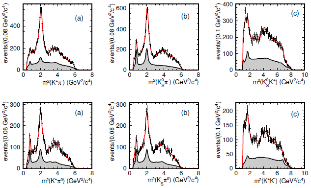
   Figure 4: (Top) $\eta_{c}\to K_{S}^{0}K^{\pm}\pi^{\mp}$ and (Bottom) $\eta_{c}\to K^{+}K^{-}\pi^{0}$ Dalitz plots projections. The superimposed curves are from the fit results. Shaded is contribution from the interpolated background.

   We note that the $K^{\ast}(892)$ contributions arise entirely from background. The fitted fractions and phases are given in Table 1. Both $\eta_{c}\to K\bar{K}\pi$ decay modes are dominated by the $(K\pi\mathcal{S}$-wave) $\bar{K}$ amplitude, with significant interference effects.

   Table 1: Results from the $\eta_{c}\to K_{S}^{0}K^{\pm}\pi^{\mp}$ and $\eta_{c}\to K^{+}K^{-}\pi^{0}$ MIPWA. Phases are determined relative to the $(K\pi\ \mathcal{S}$-wave) $\bar{K}$ amplitude which is fixed to $\pi/2$ at 1.45 GeV/c².

   	$\eta_{c}\to K_{S}^{0}K^{\pm}\pi^{\mp}$						$\eta_{c}\to K^{+}K^{-}\pi^{0}$
   Amplitude	Fraction (%)			Phase (rad)			Fraction (%)			Phase (rad)
   $(K\pi\ \mathcal{S}$-wave) $\bar{K}$	107.3 $\pm$	2.6 $\pm$	17.9		fixed		125.5 $\pm$	2.4 $\pm$	4.2		fixed
   $a_{0}(980)\pi$	0.8 $\pm$	0.5 $\pm$	0.8	1.08 $\pm$	0.18 $\pm$	0.18	0.0 $\pm$	0.1 $\pm$	1.7		-
   $a_{0}(1450)\pi$	0.7 $\pm$	0.2 $\pm$	1.4	2.63 $\pm$	0.13 $\pm$	0.17	1.2 $\pm$	0.4 $\pm$	0.7	2.90 $\pm$	0.12 $\pm$	0.25
   $a_{0}(1950)\pi$	3.1 $\pm$	0.4 $\pm$	1.2	$-$1.04 $\pm$	0.08 $\pm$	0.77	4.4 $\pm$	0.8 $\pm$	0.8	$-$1.45 $\pm$	0.08 $\pm$	0.27
   $a_{2}(1320)\pi$	0.2 $\pm$	0.1 $\pm$	0.1	1.85 $\pm$	0.20 $\pm$	0.20	0.6 $\pm$	0.2 $\pm$	0.3	1.75 $\pm$	0.23 $\pm$	0.42
   $K^{\ast}_{2}(1430)\bar{K}$	4.7 $\pm$	0.9 $\pm$	1.4	4.92 $\pm$	0.05 $\pm$	0.10	3.0 $\pm$	0.8 $\pm$	4.4	5.07 $\pm$	0.09 $\pm$	0.30
   Total	116.8 $\pm$	2.8 $\pm$	18.1				134.8 $\pm$	2.7 $\pm$	6.4
   $\chi^{2}/N_{\rm cells}$	301/254=1.17						283.2/233=1.22

   We use as figure of merit describing the fit quality the 2-D $\chi^{2}/N_{cells}$ on the Dalitz plot and obtain a good description of the data with $\chi^{2}/N_{\rm cells}=1.17$ and $\chi^{2}/N_{\rm cells}=1.22$ for the two $\eta_{c}$ decay modes.

   In comparison, the isobar model gives a worse description of the data, with $\chi^{2}/N_{cells}=457/254=1.82$ and $\chi^{2}/N_{cells}=383/233=1.63$, respectively for the two $\eta_{c}$ decay modes. The resulting $K\pi$ $\mathcal{S}$-wave amplitude and phase for the two $\eta_{c}$ decay modes is shown in Fig. 5. We observe a clear $K^{\ast}_{0}(1430)$ resonance signal with the corresponding expected phase motion. At high mass we observe the presence of the broad $K^{\ast}_{0}(1950)$ contribution with good agreement between the two $\eta_{c}$ decay modes.

   

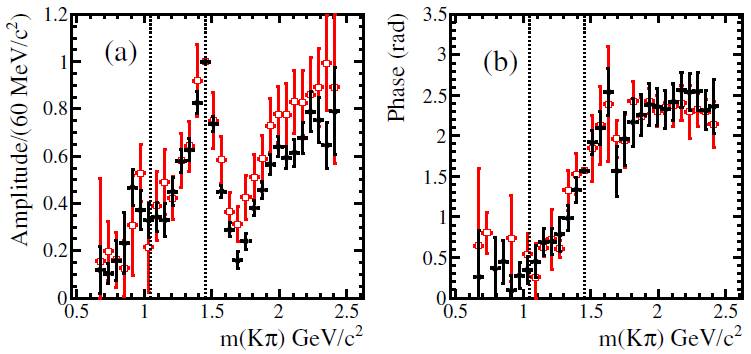
   Figure 5: The $I=1/2$ $K\pi$ $\mathcal{S}$-wave amplitude (a) and phase (b) from $\eta_{c}\to K_{S}^{0}K^{\pm}\pi^{\mp}$ (solid (black) points) and $\eta_{c}\to K^{+}K^{-}\pi^{0}$ (open (red) points); only statistical uncertainties are shown. The dotted lines indicate the $K\eta$ and $K\eta^{\prime}$ thresholds.

   Comparing with LASS [5] and E791 [4] experiments we note that phases before the $K\eta^{\prime}$ threshold are similar, as expected from Watson theorem [6] but amplitudes are very different.

   A preliminary K-matrix fit which include $K^{-}\pi^{-}\to K^{-}\pi^{-}$ $S$-wave data [7], LASS data and $\eta_{c}$ decays has been performed [8], obtaining a description of the data in terms of three-poles:

   $${\rm Pole\leavevmode\nobreak\ 1}\quad E_{P1} = \;\,659\,-\,i302\,{\rm MeV\quad on\,Sheet\,II},$$ (4)

   $${\rm Pole\leavevmode\nobreak\ 2}\quad E_{P2} = 1409\,-\,i128\,{\rm MeV\quad on\,Sheet\,III},$$ (5)

   $${\rm Pole\leavevmode\nobreak\ 3}\quad E_{P3} = 1768\,-\,i107\,{\rm MeV\quad on\,Sheet\,III}.$$ (6)

   Pole 1 is identified with the $\kappa$, the pole position of which was found to be at $[(658\pm 7)\,-\,i\ (278\pm 13)]$ MeV, in the dispersive analysis of Ref. [9]. Pole 2 is identified with $K^{\ast}_{0}(1430)$, to be compared with $[(1438\pm 8\pm 4)\,-\,i\ (105\pm 20\pm 12)]$ MeV using the Breit-Wigner form (Eq. (3)). Pole 3 may be identified with the $K^{\ast}_{0}(1950)$ with a pole mass closer to that of the reanalysis of the LASS data from Ref. [10] with a pole at $E\,=\,(1820\pm 20)\,-\,i(125\pm 50)$ MeV. For pole 2, the $K_{0}^{\ast}(1430)$, a ratio of $K\eta$/$K\pi$ decay rate of 0.05 is obtained, consistent with that reported in the present analysis (Eq. (2)).

5. Dalitz Plot Analysis of $J/\psi\to K_{S}^{0}K^{-}\pi^{\mp}$

   We study the following reaction:

   $e^{+}e^{-}\to\gamma_{\rm ISR}K_{S}^{0}K^{\pm}\pi^{\mp}$

   where $\gamma_{\rm ISR}$ indicate the ISR photon [11]. Candidate events for this reaction are selected from the sample of events having exactly four charged tracks including the $K_{S}^{0}$ candidate. We compute $M_{rec}\equiv(p_{e-}+p_{e+}-p_{K_{S}^{0}}-p_{K}-p_{\pi})^{2}$, which peaks near zero for ISR events. We select events in the ISR region by requiring $|M_{rec}^{2}|<1.5\leavevmode\nobreak\ GeV^{2}/c^{4}$ and obtain the $K_{S}^{0}K^{\pm}\pi^{\mp}$ mass spectrum shown in Fig. 6 where a clean $J/\psi$ signal can be observed.

   

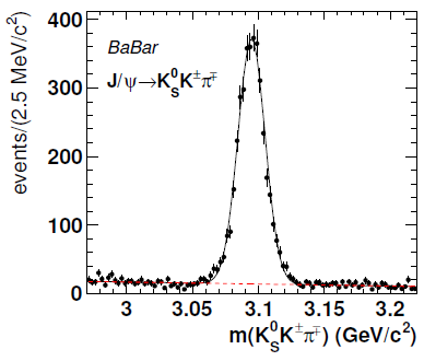
   Figure 6: $K_{S}^{0}K^{\pm}\pi^{\mp}$ mass spectrum from ISR events.

   We fit the $K_{S}^{0}K^{\pm}\pi^{\mp}$ mass spectrum using the Monte Carlo resolution functions described by a Crystal Ball+Gaussian function and obtain 3694 $\pm$ 64 events with 93.1 $\pm$ 0.4 purity.

   

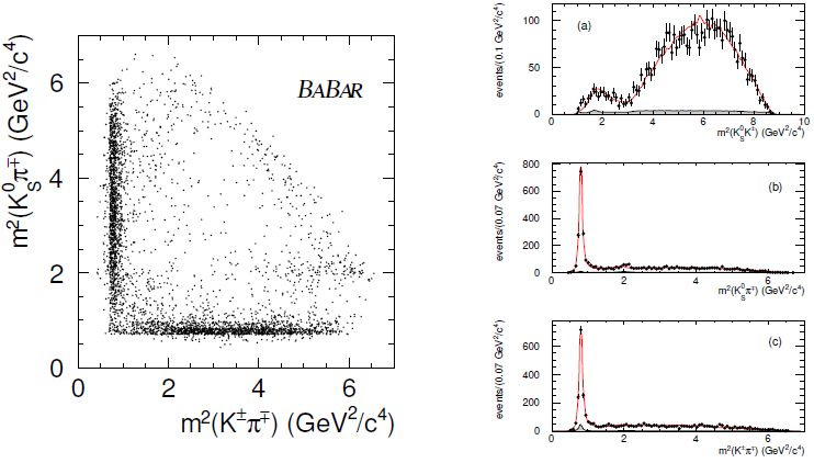
   Figure 7: (Left) $J\psi\to K_{S}^{0}K^{\pm}\pi^{\mp}$ Dalitz plot. (Right) Dalitz plot projections with fit results for $J\psi\to K_{S}^{0}K^{\pm}\pi^{\mp}$. Shaded is the background interpolated from $J\psi$ sidebands.

   Figure 7(Left) shows the Dalitz plot for the $J/\psi$ signal region and Fig. 7(Right) shows the Dalitz plot projections. We perform the Dalitz plot analysis of $J\psi\to K_{S}^{0}K^{|}pm\pi^{M}P$ using the isobar model and express the amplitudes in terms of Zemach tensors [12, 13]. We observe the following features:

   • The decay is dominated by the $K^{\ast}(892)\bar{K}$, $K^{\ast}_{2}(1430)\bar{K}$, and $\rho(1450)^{\pm}\pi^{\mp}$ amplitudes with a smaller contribution from the $K^{\ast}_{1}(1410)\bar{K}$ amplitude.

   • We obtain a significant improvement of the description of the data by leaving free the $K^{\ast}(892)$ mass and width parameters and obtain

     $$m(K^{\ast}(892)^{+})=895.6\pm 0.8\leavevmode\nobreak\ MeV/c^{2},\leavevmode\nobreak\ \leavevmode\nobreak\ \leavevmode\nobreak\ \leavevmode\nobreak\ \leavevmode\nobreak\ \leavevmode\nobreak\ \Gamma(K^{\ast}(892)^{+})=43.6\pm 1.3\leavevmode\nobreak\ MeV,$$

     $$m(K^{\ast}(892)^{0})=898.1\pm 1.0\leavevmode\nobreak\ MeV/c^{2},\leavevmode\nobreak\ \leavevmode\nobreak\ \leavevmode\nobreak\ \leavevmode\nobreak\ \leavevmode\nobreak\ \leavevmode\nobreak\ \Gamma(K^{\ast}(892)^{0})=52.6\pm 1.7\leavevmode\nobreak\ MeV.$$ (7)

   The measured parameters for the charged $K^{\ast}(892)^{+}$ are in good agreement with those measured in $\tau$ lepton decays [14].

6. Acknowledgments

   This work was supported (in part) by the U.S. Department of Energy, Office of Science, Office of Nuclear Physics under contract DE–AC05–06OR23177.

3.5 Kaon and Light-Meson Resonances at COMPASS

Boris Grube (for the COMPASS Collaboration)

Technical University Munich

85748 Garching, Germany

1. Introduction

   The excitation spectrum of light mesons is studied since many decades but is still not quantitatively understood. For higher excited meson states experimental information is often scarce or non-existent. This is in particular true for the strange-meson sector as illustrated by Fig. 1. The PDG [1] lists only 25 kaon states below 3.1 GeV: 12 states that are considered well-known and established and in addition 13 states that need confirmation. Many higher excited states that are predicted by quark-model calculation (Fig. 1 shows as an example the one from Ref. [2]) have not yet been found by experiments. In addition, for certain combinations of spin $J$ and parity $P$ the quark model does not describe the experimental data well. This is most notably the case for the scalar kaon states with $J^{P}=0^{+}$, where the $K_{0}^{\ast}(800)$ seems to be a supernumerous state.

   

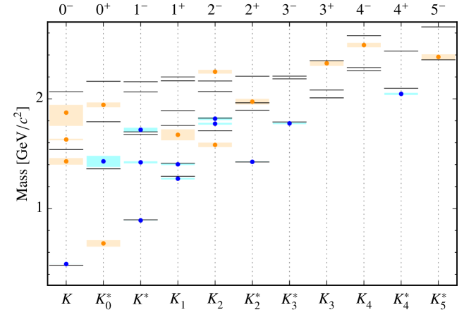
   Figure 1: Strange-meson spectrum: Comparison of the measured masses of kaon resonances (colored points with boxes representing the uncertainty) with the result of a quark-model calculation [2] (black lines). States that are considered well established by the PDG [1] are shown in blue, states that need confirmation in orange.

   In the last 30 years, little progress has been made on the exploration of the kaon spectrum. Since 1990, only four kaon states were added to the PDG and only one of them to the summary table. However, precise knowledge of the kaon spectrum is crucial to understand the light-meson spectrum. In particular, the identification of supernumerous states that could be related to new forms of matter beyond conventional quark-antiquark states—like multi-quark states, hybrids, or glueballs—requires the observation of complete SU(3)${}_{\text{flavor}}$ multiplets. The kaon spectrum also enters in analyses that search for CP violation in multi-body decays of $D$ and $B$ mesons, where kaon resonances appear in the subsystems of various final states.

2. Diffractive Production of Kaon Resonances

   A suitable reaction to produce excited kaon states is diffractive dissociation of a high-energy kaon beam, as it was already measured in the past by the WA3 experiment at CERN (see, e.g., Ref. [3]) and the LASS experiment at SLAC (see, e.g., Refs. [4, 5]). In these peripheral reactions, the beam kaon scatters softly off the target particle and is thereby excited into intermediate states, which decay into the measured $n$-body hadronic final state.

   These reactions were also measured by the COMPASS experiment using a secondary hadron beam provided by the M2 beam line of the CERN SPS. The beam was tuned to deliver negatively charged hadrons of 190 GeV momentum passing through a pair of beam Cherenkov detectors (CEDARs) for beam particle identification. The beam impinged on a 40 cm long liquid-hydrogen target with an intensity of $5\times 10^{7}$ particles per SPS spill (10 s extraction with a repetition time of about 45 s). At the target, the hadronic component of the beam consisted of 96.8% $\pi^{-}$, 2.4% $K^{-}$, and 0.8% $\bar{p}$. At the beam energy of 190 GeV, the reaction is dominated by Pomeron exchange. Elastic scattering at the target vertex was ensured by measuring the slow recoil proton. This leads to a minimum detectable reduced squared four-momentum transfer $t^{\prime}$ of about 0.07 $(\text{GeV})^{2}$. By selecting the $K^{-}$ component of the beam using the CEDAR information, we have studied diffractive production of kaon resonances. Charged kaons that appear in some of the produced forward-going final states were separated from pions by a ring-imaging Cherenkov detector (RICH) in the momentum range between 2.5 and 50 GeV.

3. Partial-Wave Analysis of $\bm{K^{-}\pi^{-}\pi^{+}}$ Final State

   In the 2008 and 2009 data-taking campaigns, COMPASS acquired a large data sample on the diffractive dissociation reaction

   $$K^{-}+p\to K^{-}\pi^{-}\pi^{+}+p.$$ (1)

   The measurement is exclusive, i.e., all four final-state particles are measured and energy-momentum conservation constraints are applied in the event selection. In reaction (1), intermediate kaon resonances are produced that decay into the 3-body $K^{-}\pi^{-}\pi^{+}$ final state. A first analysis of this reaction was performed based on a data sample that corresponds to a fraction of the available data and consists of about 270 000 events with $K^{-}\pi^{-}\pi^{+}$ mass below 2.5 GeV and in the range $0.07<t^{\prime}<0.7\leavevmode\nobreak\ (\text{GeV})^{2}$ [6, 7]. This data sample is similar in size to the one of the WA3 experiment. Fig. 2 shows selected kinematic distributions. The distribution of the energy sum of the forward-going particles peaks at the nominal beam energy. The non-exclusive background below the peak is small. The invariant mass distribution of the $K^{-}\pi^{-}\pi^{+}$ system and that of the $K^{-}\pi^{+}$ and $\pi^{-}\pi^{+}$ subsystems exhibit peaks that correspond to known resonances. All three distribution are similar to the ones obtained by WA3 [3].

   

   

   

   

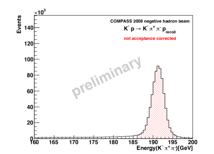
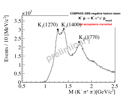
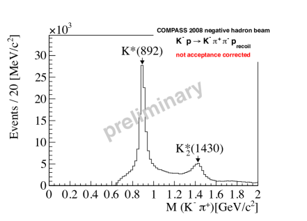
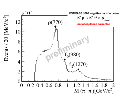
   Figure 2: Kinematic distributions [7]: (Top left) distribution of the energy sum of the forward-going particles in reaction (1), (Top right) $K^{-}\pi^{-}\pi^{+}$ invariant mass distribution, (Bottom left) $K^{-}\pi^{+}$ invariant mass distribution, and (Bottom right) $\pi^{-}\pi^{+}$ invariant mass distribution.

   As a first step towards a description of the measured $K^{-}\pi^{-}\pi^{+}$ mass spectrum in terms of kaon resonances, we performed a partial-wave analysis (PWA) using a model similar to the one used by the ACCMOR collaboration in their analysis of the WA3 data [3]. The PWA formalism is based on the isobar model and is described in detail in Ref. [8]. The PWA model takes into account three $K^{-}\pi^{+}$ isobars [$K_{0}^{\ast}(800)$, $K^{\ast}(892)$, and $K_{2}^{\ast}(1430)$] and three $\pi^{-}\pi^{+}$ isobars [$f_{0}(500)$, $\rho(770)$, and $f_{2}(1270)$]. Based on these isobars, a wave set is constructed that consists of 19 waves plus an incoherent isotropic wave, which absorbs intensity from events with uncorrelated $K^{-}\pi^{-}\pi^{+}$, e.g., non-exclusive background. A partial-wave amplitude is completely defined by the spin $J$, parity $P$, spin projection $M^{\varepsilon}$, and the decay path of the intermediate state. The spin projection is expressed in the reflectivity basis [9], where $M\geq 0$ and $\varepsilon=\pm 1$ is the naturality of the exchange particle. Since the reaction is dominated by Pomeron exchange, all waves have $\varepsilon=+1$. We use the partial-wave notation ${J}^{{P}}\allowbreak{M}^{\varepsilon}\allowbreak{\text{[isobar]}}\allowbreak{\pi}{L}$, where $L$ is the orbital angular momentum between the isobar and the third final-state particle.

   Fig. 3 shows the intensity distributions of selected waves. The ${1}^{{+}}\allowbreak{0}^{+}\allowbreak{K^{\ast}(892)}\allowbreak{\pi}{S}$ wave intensity exhibits two clear peaks at the positions of the $K_{1}(1270)$ and $K_{1}(1400)$. We also see a clear peak of the $K_{2}^{\ast}(1430)$ in the ${2}^{{+}}\allowbreak{1}^{+}\allowbreak{K^{\ast}(892)}\allowbreak{\pi}{D}$ wave intensity. However, there is no clear signal from the $K_{2}^{\ast}(1980)$. The ${2}^{{-}}\allowbreak{0}^{+}\allowbreak{K_{2}^{\ast}(1430)}\allowbreak{\pi}{S}$ wave shows a broad bump in the intensity distribution peaking slightly below 1.8 GeV that could be due to the $K_{2}(1770)$ and/or $K_{2}(1820)$. But also contributions from $K_{2}(1580)$ and/or $K_{2}(2250)$ are not excluded.

   

   

   

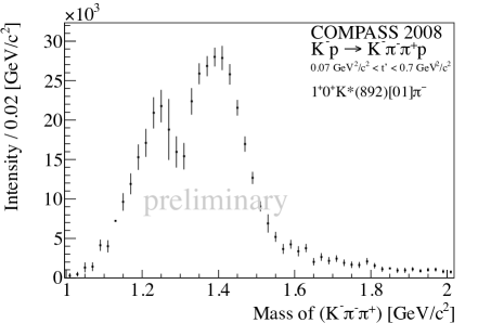
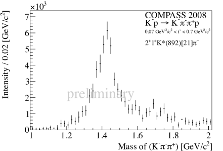
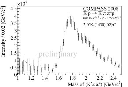
   Figure 3: Intensities of selected waves as a function of the $K^{-}\pi^{-}\pi^{+}$ mass [7]: (Top left) ${1}^{{+}}\allowbreak{0}^{+}\allowbreak{K^{\ast}(892)}\allowbreak{\pi}{S}$ wave, (Top right) ${2}^{{+}}\allowbreak{1}^{+}\allowbreak{K^{\ast}(892)}\allowbreak{\pi}{D}$ wave, and (Bottom) ${2}^{{-}}\allowbreak{0}^{+}\allowbreak{K_{2}^{\ast}(1430)}\allowbreak{\pi}{S}$ wave.

   The analysis is currently work in progress. With an improved beam particle identification and event selection the full data sample consists of about 800 000 exclusive events, making it the world’s larges data set of this kind. Also the PWA model will be improved by using more realistic isobar parametrizations and parameters and by including the $f_{0}(980)$ as an additional $\pi^{-}\pi^{+}$ isobar. In order to extract kaon resonances and their parameters, we will also perform a resonance-model fit similar to the one of the $\pi^{-}\pi^{-}\pi^{+}$ final state in Ref. [10].

4. Possible Future Measurements with Kaon Beam

   The COMPASS collaboration has submitted a proposal for a future fixed-target experiment within in the framework of CERN’s “Physics beyond Colliders” initiative. Among other things, we propose to perform a high-precision measurement of the kaon spectrum using a high-energy kaon beam similar to the COMPASS measurements in 2008 and 2009. The goal of this experiment would be to acquire a high-precision data set that is at least 10 times larger than that of COMPASS. Such a large data set would allow us not only to search for small signals but also to apply the novel analysis techniques that we developed for the analysis of the COMPASS $\pi^{-}\pi^{-}\pi^{+}$ data sample, which consists of $46\times 10^{6}$ events [8, 10, 11]. In particular, we could study in detail the amplitude of the scalar $K^{-}\pi^{+}$ subsystem with $J^{P}=0^{+}$ in the the $K^{-}\pi^{-}\pi^{+}$ final state as a function of the $K^{-}\pi^{+}$ mass, the $K^{-}\pi^{-}\pi^{+}$ mass, and the quantum numbers of the $K^{-}\pi^{-}\pi^{+}$ system, similar to the analysis of the scalar $\pi^{-}\pi^{+}$ subsystem in the $\pi^{-}\pi^{-}\pi^{+}$ final state in Ref. [8]. With these data, one could learn more about the scalar kaon states. The PWA could also be performed in bins of the reduced squared four-momentum $t^{\prime}$ in order to extract the $t^{\prime}$ dependence of the resonant and non-resonant partial-wave components like it was done for the $\pi^{-}\pi^{-}\pi^{+}$ final state in Ref. [10]. This gives information about the production processes.

   To obtain such a high-precision data set for kaon spectroscopy, the rate of beam kaons on the target must be increased with respect to the COMPASS measurements in 2008 and 2009. This can be achieved by increasing the kaon fraction in the beam using RF-separation techniques [12, 13] similar to the ones that have already been used in the past at CERN [14] (see Fig. 4). First preliminary estimates for the M2 beam line at CERN show that a high-energy kaon beam with a kaon rate of about $3.7\times 10^{6}$ s^-1 seems to be feasible [15, 16]. This would correspond to about 10 to $20\times 10^{6}$ $K^{-}\pi^{-}\pi^{+}$ events within a year of running. However, more detailed feasibility studies are still needed.

   

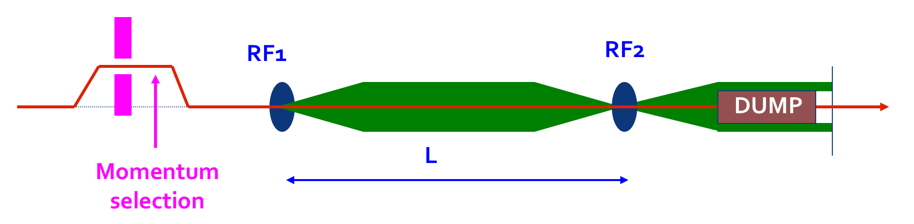
   Figure 4: Principle of an RF-separated beam [15]: A momentum-selected beam passes through two RF-cavities that act as a time-of-flight selector. The first RF-cavity deflects the beam. This deflection is cancelled or enhanced by the second RF-cavity, depending on the particle type. Hence particles can be selected in the plane transverse to the beam by putting absorbers or collimators.

5. Acknowledgments

   This work was supported by the BMBF, the Maier-Leibnitz-Laboratorium (MLL), the DFG Cluster of Excellence Exc153 “Origin and Structure of the Universe,” and the computing facilities of the Computational Center for Particle and Astrophysics (C2PAP).

3.6 Recent Belle Results Related to $\pi-K$ Interactions

Bilas Pal (for the Belle Collaboration)

Brookhaven National Laboratory

Upton, NY 11973, U.S.A. &

University of Cincinnati

Cincinnati, OH, U.S.A

1. Introduction

   In this report, we present some recent results related to $\pi-K$ interactions based on the data, collected by the Belle experiment at the KEKB $e^{+}e^{-}$ asymmetric-energy collider [1]. (Throughout this paper charge-conjugate modes are implied.) The experiment took data at center-of-mass energies corresponding to several $\Upsilon(nS)$ resonances; the total data sample recorded exceeds $1\leavevmode\nobreak\ {\rm ab}^{-1}$.

   The Belle detector is a large-solid-angle magnetic spectrometer that consists of a silicon vertex detector (SVD), a 50-layer central drift chamber (CDC), an array of aerogel threshold Cherenkov counters (ACC), a barrel-like arrangement of time-of-flight scintillation counters (TOF), and an electromagnetic calorimeter comprised of CsI(Tl) crystals (ECL) located inside a super-conducting solenoid coil that provides a 1.5 T magnetic field. An iron flux-return located outside of the coil is instrumented to detect $K^{0}_{L}$ mesons and to identify muons (KLM). The detector is described in detail elsewhere [2, 3].

2. $CP$ Asymmetry in $B^{+}\to K^{+}K^{-}\pi^{+}$ Decays

   In the recent years, an unidentified structure has been observed by BaBar [4] and LHCb experiments [5, 6] in the low $K^{+}K^{-}$ invariant mass spectrum of the $B^{+}\to K^{+}K^{-}\pi^{+}$ decays. The LHCb reported a nonzero inclusive $CP$ asymmetry of $-0.123\pm 0.017\pm 0.012\pm 0.007$ and a large unquantified local $CP$ asymmetry in the same mass region. These results suggest that final-state interactions may contribute to $CP$ violation [7, 8]. In this analysis, we attempt to quantify the $CP$ asymmetry and branching fraction as a function of the $K^{+}K^{-}$ invariant mass, using $711\leavevmode\nobreak\ {\rm fb^{-1}}$ of data, collected at $\Upsilon(4S)$ resonance [9].

   The signal yield is extracted by performing a two-dimensional unbinned maximum likelihood fit to the variables: the beam-energy constrained mass $M_{\rm bc}$ and the energy difference $\Delta E$. The resulting branching fraction and $CP$ asymmetry are

   $$\mathcal{B}(B^{+}\to K^{+}K^{-}\pi^{+}) = (5.38\pm 0.40\pm 0.35)\times 10^{-6},$$

   $$A_{CP} = -0.170\pm 0.073\pm 0.017,$$

   where the quoted uncertainties are statistical and systematic, respectively.

   To investigate the localized $CP$ asymmetry in the low $K^{+}K^{-}$ invariant mass region, we perform the 2D fit (described above) to extract the signal yield and $A_{CP}$ in bins of $M_{K^{+}K^{-}}$. The fitted results are shown in Fig. 1 and Table 1. We confirm the excess and local $A_{CP}$ in the low $M_{K^{+}K^{-}}$ region, as reported by the LHCb, and quantify the differential branching fraction in each $K^{+}K^{-}$ invariant mass bin. We find a 4.8$\sigma$ evidence for a negative $CP$ asymmetry in the region $M_{K^{+}K^{-}}<1.1$ GeV/$c^{2}$. To understand the origin of the low-mass dynamics, a full Dalitz analysis from experiments with a sizeable data set, such as LHCb and Belle II, will be needed in the future.

   

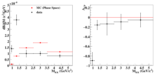
   Figure 1: Differential branching fractions (left) and measured $A_{CP}$ (right) as a function of $M_{K^{+}K^{-}}$. Each point is obtained from a two-dimensional fit with systematic uncertainty included. Red squares with error bars in the left figure show the expected signal distribution in a three-body phase space MC. Note that the phase space hypothesis is rescaled to the total observed $K^{+}K^{-}\pi^{+}$ signal yield.

   Table 1: Differential branching fraction, and $A_{CP}$ for individual $M_{K^{+}K^{-}}$ bins. The first uncertainties are statistical and the second systematic.

   $M_{K^{+}K^{-}}$	$d\mathcal{B}/dM(\times 10^{-7})$	$A_{CP}$
   0.8–1.1	$14.0\pm 2.7\pm 0.8$	$-0.90\pm 0.17\pm 0.04$
   1.1–1.5	$37.8\pm 3.8\pm 1.9$	$-0.16\pm 0.10\pm 0.01$
   1.5–2.5	$10.0\pm 2.3\pm 1.7$	$-0.15\pm 0.23\pm 0.03$
   2.5–3.5	$10.0\pm 1.6\pm 0.6$	$-0.09\pm 0.16\pm 0.01$
   3.5–5.3	$8.1\pm 1.2\pm 0.5$	$-0.05\pm 0.15\pm 0.01$

3. Search for $\Lambda_{c}^{+}\to\phi p\pi^{0}$ and Branching Fraction Measurement of $\Lambda_{c}^{+}\to K^{-}\pi^{+}p\pi^{0}$

   The story of exotic hadron spectroscopy begins with the discovery of the $X(3872)$ by the Belle collaboration in 2003 [10]. Since then, many exotic $X\!Y\!Z$ states have been reported by Belle and other experiments [11]. Recent observations of two hidden-charm pentaquark states $P_{c}^{+}(4380)$ and $P_{c}^{+}(4450)$ by the LHCb collaboration in the $J/\psi p$ invariant mass spectrum of the $\Lambda_{b}^{0}\to J/\psi pK^{-}$ process [12] raises the question of whether a hidden-strangeness pentaquark $P_{s}^{+}$, where the $c\bar{c}$ pair in $P_{c}^{+}$ is replaced by an $s\bar{s}$ pair, exists [14, 13, 15]. The strange-flavor analogue of the $P_{c}^{+}$ discovery channel is the decay $\Lambda_{c}^{+}\to\phi p\pi^{0}$ [14, 15], shown in Fig. 2 (a). The detection of a hidden-strangeness pentaquark could be possible through the $\phi p$ invariant mass spectrum within this channel [see Fig. 2 (b)] if the underlying mechanism creating the $P_{c}^{+}$ states also holds for $P_{s}^{+}$, independent of the flavor [15], and only if the mass of $P_{s}^{+}$ is less than $M_{\Lambda_{c}^{+}}-M_{\pi^{0}}$. In an analogous $s\bar{s}$ process of $\phi$ photoproduction $(\gamma p\to\phi p)$, a forward-angle bump structure at $\sqrt{s}\approx 2.0$ GeV has been observed by the LEPS [16] and CLAS collaborations [17]. However, this structure appears only at the most forward angles, which is not expected for the decay of a resonance [18].

   

   

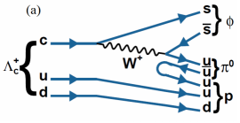
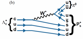
   Figure 2: Feynman diagram for the decay (a) $\Lambda_{c}^{+}\to\phi p\pi^{0}$ and (b) $\Lambda_{c}^{+}\to P_{s}^{+}\pi^{0}$.

   Previously, the decay $\Lambda_{c}^{+}\to\phi p\pi^{0}$ has not been studied by any experiment. Here, we report a search for this decay, using 915 $\rm fb^{-1}$ of data [19]. In addition, we search for the nonresonant decay $\Lambda_{c}^{+}\to K^{+}K^{-}p\pi^{0}$ and measure the branching fraction of the Cabibbo-favored decay $\Lambda_{c}^{+}\to K^{-}\pi^{+}p\pi^{0}$.

   In order to extract the signal yield, we perform a two-dimensional (2D) unbinned extended maximum likelihood fit to the variables $m(K^{+}K^{-}p\pi^{0})$ and $m(K^{+}K^{-})$. Projections of the fit result are shown in Fig. 3. From the fit, we extract $148.4\pm 61.8$ signal events, $75.9\pm 84.8$ nonresonant events, and $7158.4\pm 36.4$ combinatorial background events. The statistical significances are found to be 2.4 and 1.0 standard deviations for $\Lambda_{c}^{+}\to\phi p\pi^{0}$ and nonresonant $\Lambda_{c}^{+}\to K^{+}K^{-}p\pi^{0}$ decays, respectively. We use the well-established decay $\Lambda_{c}^{+}\to pK^{-}\pi^{+}$ [11] as the normalization channel for the branching fraction measurements.

   

   

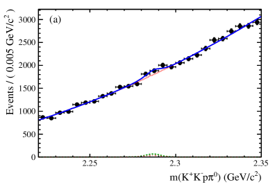
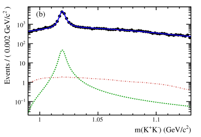
   Figure 3: Projections of the 2D fit: (a) $m(K^{+}K^{-}p\pi^{0})$ and (b) $m(K^{+}K^{-})$. The points with the error bars are the data, and the (red) dotted, (green) dashed and (brown) dot-dashed curves represent the combinatorial, signal and nonresonant candidates, respectively, and (blue) solid curves represent the total PDF. The solid curve in (b) completely overlaps the curve for the combinatorial background.

   Since the significances are below 3.0 standard deviations both for $\phi p\pi^{0}$ signal and $K^{+}K^{-}p\pi^{0}$ nonresonant decays, we set upper limits on their branching fractions at 90% confidence level (CL) using a Bayesian approach. The results are

   $$\mathcal{B}(\Lambda_{c}^{+}\to\phi p\pi^{0}) < 15.3\times 10^{-5},$$

   $$\mathcal{B}(\Lambda_{c}^{+}\to K^{+}K^{-}p\pi^{0})_{\rm NR} < 6.3\times 10^{-5},$$

   which are the first limits on these branching fractions.

   To search for a putative $P_{s}^{+}\to\phi p$ decay, we select $\Lambda_{c}^{+}\to K^{+}K^{-}p\pi^{0}$ candidates in which $m(K^{+}K^{-})$ is within 0.020 GeV/$c^{2}$ of the $\phi$ meson mass [11] and plot the background-subtracted $m(\phi p)$ distribution (Fig. 4). This distribution is obtained by performing 2D fits as discussed above in bins of $m(\phi p)$. The data shows no clear evidence for a $P_{s}^{+}$ state. We set an upper limit on the product branching fraction $\mathcal{B}(\Lambda_{c}^{+}\to P_{s}^{+}\pi^{0})\times\mathcal{B}(P_{s}^{+}\to\phi p)$ by fitting the distribution of Fig. 4 to the sum of a RBW function and a phase space distribution determined from a sample of simulated $\Lambda^{+}_{c}\to\phi p\pi^{0}$ decays. We obtain $77.6\pm 28.1$ $P_{s}^{+}$ events from the fit, which gives an upper limit of

   $$\mathcal{B}(\Lambda_{c}^{+}\to P_{s}^{+}\pi^{0})\times\mathcal{B}(P_{s}^{+}\to\phi p)<8.3\times 10^{-5}$$

   at 90% CL. for our limit on ${\cal B}(\Lambda_{c}^{+}\rightarrow\phi p\pi^{0})$. From the fit, we also obtain, $M_{P_{s}^{+}}=(2.025\pm 0.005)$ GeV/$c^{2}$ and $\Gamma_{P_{s}^{+}}=(0.022\pm 0.012)$ GeV, where the uncertainties are statistical only.

   

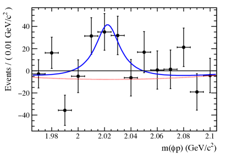
   Figure 4: The background-subtracted distribution of $m(\phi p)$ in the $\phi p\pi^{0}$ final state. The points with error bars are data, and the (blue) solid line shows the total PDF. The (red) dotted curve shows the fitted phase space component (which has fluctuated negative).

   The high statistics decay $\Lambda_{c}^{+}\to K^{-}\pi^{+}p\pi^{0}$ is used to adjust the data-MC differences in the $\phi p\pi^{0}$ signal and $K^{+}K^{-}p\pi^{0}$ nonresonant decays. For the $\Lambda_{c}^{+}\to K^{-}\pi^{+}p\pi^{0}$ sample, the mass distribution is plotted in Fig. 5. We fit this distribution to obtain the signal yield. We find $242\,039\pm\,2342$ signal candidates and $472\,729\pm\,467$ background candidates. We measure the ratio of branching fractions,

   $$\frac{\mathcal{B}(\Lambda_{c}^{+}\to K^{-}\pi^{+}p\pi^{0})}{\mathcal{B}(\Lambda_{c}^{+}\to K^{-}\pi^{+}p)}=(0.685\pm 0.007\pm 0.018),$$

   where the first uncertainty is statistical and the second is systematic. Multiplying this ratio by the world average value of $\mathcal{B}(\Lambda_{c}^{+}\to K^{-}\pi^{+}p)=(6.46\pm 0.24)\%$ [20], we obtain

   $$\mathcal{B}(\Lambda_{c}^{+}\to K^{-}\pi^{+}p\pi^{0})=(4.42\pm 0.05\pm 0.12\pm 0.16)\%,$$

   where the first uncertainty is statistical, the second is systematic, and the third reflects the uncertainty due to the branching fraction of the normalization decay mode. This is the most precise measurement of $\mathcal{B}(\Lambda_{c}^{+}\to K^{-}\pi^{+}p\pi^{0})$ to date and is consistent with the recently measured value $\mathcal{B}(\Lambda_{c}^{+}\to K^{-}\pi^{+}p\pi^{0})=(4.53\pm 0.23\pm 0.30)\%$ by the BESIII collaboration [21].

   

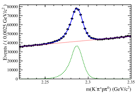
   Figure 5: Fit to the invariant mass distribution of $m(K^{-}\pi^{+}p\pi^{0})$. The points with the error bars are the data, the (red) dotted and (green) dashed curves represent the combinatorial and signal candidates, respectively, and (blue) curve represents the total PDF. of bins) of the fit is 1.43, which indicate that the fit gives a good description of the data.

4. Observation of the Doubly Cabibbo-Suppressed $\Lambda_{c}^{+}$ Decay

   Several doubly Cabibbo-suppressed (DCS) decays of charmed mesons have been observed [11]. Their measured branching ratios with respect to the corresponding Cabibbo-favored (CF) decays play an important role in constraining models of the decay of charmed hadrons and in the study of flavor- $SU(3)$ symmetry [22, 23]. On the other hand, because of the smaller production cross-sections for charmed baryons, DCS decays of charmed baryons have not yet been observed, and only an upper limit, $\frac{\mathcal{B}(\Lambda_{c}^{+}\to pK^{+}\pi^{-})}{\mathcal{B}(\Lambda_{c}^{+}\to pK^{-}\pi^{+})}<0.46\%$ at 90% CL, has been reported by the FOCUS Collaboration [24]. Here we present the first observation of the DCS decay $\Lambda_{c}^{+}\to pK^{+}\pi^{-}$ and the measurement of its branching ratio with respect to the CF decay $\Lambda_{c}^{+}\to pK^{-}\pi^{+}$, using $980\leavevmode\nobreak\ {\rm fb}^{-1}$ of data [25].

   Figure 6 shows the invariant mass distributions of (a) $pK^{-}\pi^{+}$ (CF) and (b) $pK^{+}\pi^{-}$ (DCS) combinations. DCS decay events are clearly observed in $M(pK^{+}\pi^{-})$. In order to obtain the signal yield, a binned least-$\chi^{2}$ fit is performed. From the mass fit, we extract $(1.452\pm 0.015)\times 10^{6}$ $\Lambda_{c}^{+}\to pK^{-}\pi^{+}$ events and $3587\pm 380$ $\Lambda_{c}^{+}\to pK^{+}\pi^{-}$ events. The latter has a peaking background from the single Cabibbo-suppressed (SCS) decay $\Lambda_{c}^{+}\to\Lambda(\to p\pi^{-})K^{+}$, which has the same final-state topology. After subtracting the SCS contribution, we have $3379\pm 380\pm 78$ DCS events, where the first uncertainty is statistical and the second is the systematic due to SCS subtraction. The corresponding statistical significance is 9.4 standard deviations. We measure the branching ratio,

   $$\frac{\mathcal{B}(\Lambda_{c}^{+}\to pK^{+}\pi^{-})}{\mathcal{B}(\Lambda_{c}^{+}\to pK^{-}\pi^{+})}=(2.35\pm 0.27\pm 0.21)\times 10^{-3},$$

   where the uncertainties are statistical and systematic, respectively. This measured branching ratio corresponds to $(0.82\pm 0.21)\tan^{4}\theta_{c}$, where the uncertainty is the total, which is consistent within 1.5 standard deviations with the naïve expectation ($\sim\tan^{4}\theta_{c}$ [24]). LHCb’s recent measurement of $\frac{\mathcal{B}(\Lambda_{c}^{+}\to pK^{+}\pi^{-})}{\mathcal{B}(\Lambda_{c}^{+}\to pK^{-}\pi^{+})}=(1.65\pm 0.15\pm 0.05)\times 10^{-3}$ [26] is lower than our ratio at the 2.0$\sigma$ level. Multiplying this ratio with the previously measured $\mathcal{B}(\Lambda_{c}^{+}\to pK^{-}\pi^{+})=(6.84\pm 0.24^{+0.21}_{-0.27})\%$ by the Belle Collaboration [27], we obtain the the absolute branching fraction of the DCS decay,

   $$\mathcal{B}(\Lambda_{c}^{+}\to pK^{+}\pi^{-})=(1.61\pm 0.23^{+0.07}_{-0.08})\times 10^{-4},$$

   where the first uncertainty is due to the total uncertainty of the branching ratio and the second is uncertainty due to the branching fraction of the CF decay. After subtracting the contributions of $\Lambda^{\ast}(1520)$ and $\Delta$ isobar intermediates, which contribute only to the CF decay, the revised ratio, $\frac{\mathcal{B}(\Lambda_{c}^{+}\to pK^{+}\pi^{-})}{\mathcal{B}(\Lambda_{c}^{+}\to pK^{-}\pi^{+})}=(1.10\pm 0.17)\tan^{4}\theta_{c}$ is consistent with the naïve expectation within 1.0 standard deviation.

   

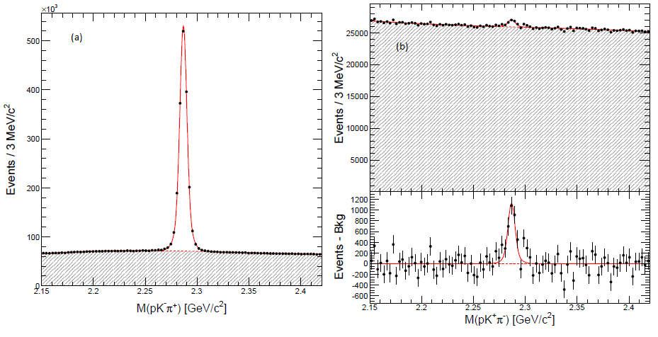
   Figure 6: Distributions of (a) $M(pK^{-}\pi^{+})$ and (b) $M(pK^{+}\pi^{-})$ and residuals of data with respect to the fitted combinatorial background. The solid curves indicate the full fit model and the dashed curves the combinatorial background.

5. $\phi_{3}$ Measurement with a Model-independent Dalitz Plot Analysis of $B^{\pm}\to DK^{\pm},D\to K_{S}^{0}\pi^{+}\pi^{-}$ Decay

   The CKM angle $\phi_{3}$ (also denoted as $\gamma$) is one of the least constrained parameters of the CKM Unitary Triangle. Its determination is however theoretically clean due to absence of loop contributions; $\phi_{3}$ can be determined using tree-level processes only, exploiting the interference between $b\to u\bar{c}s$ and $b\to c\bar{u}s$ transitions that occurs when a process involves a neutral $D$ meson reconstructed in a final state accessible to both $D^{0}$ and $\bar{D}^{0}$ decays (see Fig. 7). Therefore, the angle $\phi_{3}$ provides a SM benchmark, and its precise measurement is crucial in order to disentangle non-SM contributions to other processes, via global CKM fits. The size of the interference also depends on the ratio ($r_{B}$) of the magnitudes of the two tree diagrams involved and $\delta_{B}$, the strong phase difference between them. Those hadronic parameters will be extracted from data together with the angle $\phi_{3}$.

   

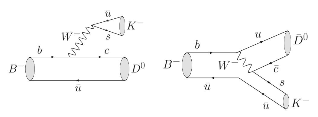
   Figure 7: Feynman diagram for $B^{-}\to D^{0}K^{-}$ and $B^{-}\to\bar{D}^{0}K^{-}$ decays.

   The measurement are performed in three different ways: (a) by utilizing decays of $D$ mesons to $CP$ eigenstates, such as $\pi^{+}\pi^{-}$, $K^{+}K^{-}$ ($CP$ even) or $K_{S}^{0}\pi^{0}$, $\phi K_{S}^{0}$ ($CP$ odd), proposed by Gronau, London, and Wyler (and called the GLW method [28, 29]) (b) by making use of DCS decays of $D$ mesons, $e.g.$, $D^{0}\to K^{+}\pi^{-}$, proposed by Atwood, Dunietz, and Soni (and called the ADS method [30]) and (c) by exploiting the interference pattern in the Dalitz plot of the $D$ decays such as $D^{0}\to K_{S}^{0}\pi^{+}\pi^{-}$, proposed by Giri, Grossman, Soffer, and Zupanc (and called the GGSZ method [31]).

   Using a model-dependent Dalitz plot method, Belle’s earlier measurement [32] based on a data sample of $605\leavevmode\nobreak\ {\rm fb^{-1}}$ integrated luminosity yielded $\phi_{3}=(78.4^{+10.8}_{-11.6}\pm 3.6\pm 8.9)^{\circ}$ and $r_{B}=0.160^{+0.040}_{-0.038}\pm 0.011^{+0.050}_{-0.010}$, where the uncertainties are statistical, systematic and Dalitz model dependence, respectively. Although with more data one can squeeze on the statistical part, the result will still remain limited by the model uncertainty.

   In a bid to circumvent this problem, Belle has carried out a model-independent analysis [33], using GGSZ method [31], that is further extended in a latter work [34]. The analysis is based on the $711\leavevmode\nobreak\ {\rm fb^{-1}}$ of data, collected at the $\Upsilon(4S)$ resonance. In contrast to the conventional Dalitz method, where the $D^{0}\to K_{S}^{0}\pi^{+}\pi^{-}$ amplitudes are parameterized as a coherent sum of several quasi two-body amplitudes as well as a nonresonant term, the model-independent approach invokes study of a binned Dalitz plot. In this approach, the expected number of events in the $i^{th}$ bin of the Dalitz plan for the $D$ mesons from $B^{\pm}\to DK^{\pm}$ is given by where $h_{B}$ is the overall normalization and $K_{i}$ is the number of events in the $i^{th}$ Dalitz bin of the flavor-tagged (whether $D^{0}$ or $\bar{D}^{0}$) $D^{0}\to K_{S}^{0}\pi^{+}\pi^{-}$ decays, accessible via the charge of the slow pion in $D^{\ast\pm}\to D\pi^{\pm}$. The terms $c_{i}$ and $s_{i}$ contain information about the strong-phase difference between the symmetric Dalitz points [$m^{2}(K_{S}^{0}\pi^{+}),\leavevmode\nobreak\ m^{2}(K_{S}^{0}\pi^{-})$] and [$m^{2}(K_{S}^{0}\pi^{-}),\leavevmode\nobreak\ m^{2}(K_{S}^{0}\pi^{+})$]; they are the external inputs obtained from quantum correlated $D^{0}\bar{D^{0}}$ decays at the $\psi(3770)$ resonance in CLEO [35, 36]. Finally $x_{\pm}=r_{B}\cos(\delta_{B}\pm\phi_{3})$ and $y_{\pm}=r_{B}\sin(\delta_{B}\pm\phi_{3})$, where $\delta_{B}$ is the strong-phase difference between $B^{\pm}\to\bar{D}^{0}K^{\pm}$ and $B^{\pm}\to D^{0}K^{\pm}$.

   We perform a combined likelihood fit to four signal selection variables in all Dalitz bins (16 bins in our case) for the $B^{\pm}\to DK^{\pm}$ signal and Cabibbo-favored $B^{\pm}\to D\pi^{\pm}$ control samples; the free parameters of the fit are $x_{\pm}$, $y_{\pm}$, overall normalization (see Eq. 1) and background fraction. Table 2 summarizes the results obtained for $B^{\pm}\to DK^{\pm}$ decays. From these results, we obtain $\phi_{3}=(77.3^{+15.1}_{-14.9}\pm 4.1\pm 4.3)^{\circ}$ and $r_{B}=0.145\pm 0.030\pm 0.010\pm 0.011$, where the first error is statistical, the second is systematic, and the last error is due to limited precision on $c_{i}$ and $s_{i}$. Although $\phi_{3}$ has a mirror solution at $\phi_{3}+180^{\circ}$, we retain the value consistent with $0^{\circ}<\phi_{3}<180^{\circ}$.

   Table 2: Results of the $x,y$ parameters and their statistical correlation for $B^{\pm}\to DK^{\pm}$ decays. The quoted uncertainties are statistical, systematic, and precision on $c_{i}$, $s_{i}$, respectively.

   Parameter
   $x_{+}$	$+0.095\pm 0.045\pm 0.014\pm 0.010$
   $y_{+}$	$+0.135^{+0.053}_{-0.057}\pm 0.015\pm 0.023$
   corr($x_{+}$, $y_{+}$)	-0.315
   $x_{-}$	$-0.110\pm 0.043\pm 0.014\pm 0.007$
   $y_{-}$	$-0.050^{+0.052}_{-0.055}\pm 0.011\pm 0.017$
   corr($x_{-}$, $y_{-}$)	+0.059

   We report evidence for direct $CP$ violation, the fact that $\phi_{3}$ is nonzero, at the 2.7 standard deviations level. Compared to results of the model-dependent Dalitz method, this measurement has somewhat poorer statistical precision despite a larger data sample used. There are two factors responsible for lower statistical sensitivity: 1) the statistical error for the same statistics is inversely proportional to the $r_{B}$ value, and the central value of $r_{B}$ in this analysis is smaller, and 2) the binned approach is expected to have the statistical precision that is, on average, 10–20% poorer than the unbinned one. On the positive side, however, the large model uncertainty for the model-dependent study ($8.9^{\circ}$) is now replaced by a purely statistical uncertainty due to limited size of the $\psi(3770)$ data sample available at CLEO ($4.3^{\circ}$). With the use of BES-III data, this error will decrease to $1^{\circ}$ or less.

   The model-independent approach therefore offers an ideal avenue for Belle II and LHCb in their pursuits of $\phi_{3}$. We expect that the statistical error of the $\phi_{3}$ measurement using the statistics of a $50\leavevmode\nobreak\ {\rm ab^{-1}}$ data sample that will be available at Belle II will reach $1-2^{\circ}$. We also expect that the experimental systematic error can be kept at the level below $1^{\circ}$, since most of its sources are limited by the statistics of the control channels.

6. Acknowledgments

   The author thanks the organizers of PKI2018 for excellent hospitality and for assembling a nice scientific program. This work is supported by the U.S. Department of Energy.

3.7 Study of $\tau\to K\pi\nu$ Decay at the B Factories

Denis Epifanov

Budker Institute of Nuclear Physics SB RAS

Novosibirsk, 630090 Russia

1. Introduction

   The record statistics of $\tau$ leptons collected at the $e^{+}e^{-}$ $B$ factories [1] provide unique opportunities of the precision tests of the Standard Model (SM). In the SM, $\tau$ decays due to the charged weak interaction described by the exchange of $W$ boson. Hence, there are two main classes of $\tau$ decays, leptonic and hadronic $\tau$ decays. Leptonic decays provide very clean laboratory to probe electroweak couplings [2], while hadronic $\tau$ decays offer unique tools for the precision study of low energy QCD [3]. The hadronic system is produced from the QCD vacuum via decay of the $W^{-}$ boson into $\bar{u}$ and $d$ quarks (Cabibbo-allowed decays) or $\bar{u}$ and $s$ quarks (Cabibbo-suppressed decays). As a result the decay amplitude can be factorized into a purely leptonic part including the $\tau^{-}$ and $\nu_{\tau}$ and a hadronic spectral function.

   Of particular interest are strangeness changing Cabibbo-suppressed hadronic $\tau$ decays. The decays $\tau^{-}\to\bar{K^{0}}\pi^{-}\nu_{\tau}$ and $\tau^{-}\to K^{-}\pi^{0}\nu_{\tau}$ (or, shortly, $\tau\to K\pi\nu$) provide the dominant contribution to the inclusive strange hadronic spectral function, which is used to evaluate $s$-quark mass and $V_{us}$ element of Cabibbo-Kobayashi-Maskawa (CKM) quark flavor-mixing matrix [4]. In the $\tau\to K\pi\nu$ decays the $K\pi$ system is produced in the clean experimental conditions without disturbance from the final state interactions. Hence, $\tau\to K\pi\nu$ decays provide complementary information about $K$-$\pi$ interaction to the experiments with kaon beams [5, 6]. In the leptonic sector, CP symmetry violation (CPV) is strongly suppressed in the SM ($A_{\rm SM}^{\rm CP}\lesssim 10^{-12}$) leaving enough room to search for the effects of New Physics [7]. Of particular interest are strangeness changing Cabibbo-suppressed hadronic $\tau$ decays, in which large CPV could appear from a charged scalar boson exchange in some Multi-Higgs-Doublet models (MHDM) [8].

   Recently, Belle and BaBar performed an extended study of the $\tau\to K\pi\nu$ decays and searches for CPV in these decays [9, 10, 11, 12, 13, 14].

2. Study of $\tau\to K\pi\nu$ Decays at Belle and BaBar

   The first analysis of $\tau^{-}\to K^{0}_{S}\pi^{-}\nu_{\tau}$ decay at Belle was done with a $351\leavevmode\nobreak\ {\rm fb}^{-1}$ data sample that contains $323\times 10^{6}\ \tau^{+}\tau^{-}$ pairs [9]. So called lepton-tagged events were selected, in which $\tau^{+}$ decays to leptons, $\tau^{+}\to\ell^{+}\nu_{\ell}\bar{\nu_{\tau}},\leavevmode\nobreak\ \ell=e,\,\mu$, while the other one decays to the signal $K^{0}_{S}\pi^{-}\nu_{\tau}$ final state. Events where both $\tau$’s decay to leptons were used for the normalization. In the calculation of the $\tau^{-}\to K^{0}_{S}\pi^{-}\nu_{\tau}$ branching fraction the detection efficiencies for the signal and two-lepton events were determined from Monte Carlo (MC) simulation with the corrections from the experimental data. The obtained branching fraction:

   $${\cal B}(\tau^{-}\to K^{0}_{S}\pi^{-}\nu_{\tau})=(4.04\pm 0.02({\rm stat.})\pm 0.13({\rm syst.}))\times 10^{-3}$$

   is consistent with the other measurements.

   

   

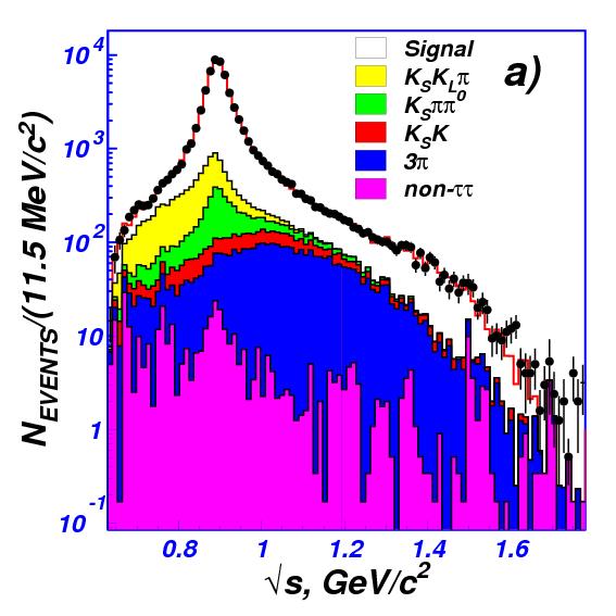
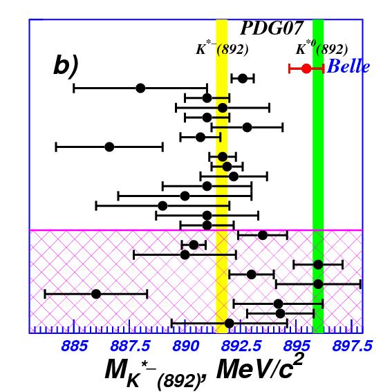
   Figure 1: (a) The $K^{0}_{S}\pi$ mass distribution, points are experimental data, the histogram is the $K_{0}^{\ast}(800)^{-}+K^{\ast}(892)^{-}+K^{\ast}(1410)^{-}$ model; (b) The $K^{\ast}(892)^{-}$ mass measured in different experiments.

   The $K^{0}_{S}\pi^{-}$ invariant mass distribution shown in Fig. 1 (a) is described in terms of the vector ($F_{V}$) and the scalar ($F_{S}$) form factors according to Ref. [16]:

   $$\frac{d\Gamma}{d\sqrt{s}}\sim\frac{1}{s}\biggl{(}1-\frac{s}{m^{2}_{\tau}}\biggr{)}^{2}\biggl{(}1+2\frac{s}{m^{2}_{\tau}}\biggr{)}P\biggl{\{}P^{2}|F_{V}|^{2}+\frac{3(m^{2}_{K}-m^{2}_{\pi})^{2}}{4s(1+2\frac{s}{m^{2}_{\tau}})}|F_{S}|^{2}\biggr{\}},$$ (1)

   where $s$ is squared $K^{0}_{S}\pi^{-}$ invariant mass, $P$ is $K^{0}_{S}$ momentum in the $K^{0}_{S}\pi^{-}$ rest frame. The vector form factor is parametrized by the $K^{\ast}(892)^{-}$, $K^{\ast}(1410)^{-}$ and $K^{\ast}(1680)^{-}$ meson amplitudes, while the scalar form factor includes the $K_{0}^{\ast}(800)^{-}$ and $K_{0}^{\ast}(1430)^{-}$ contributions. The $K^{\ast}(892)^{-}$ alone is not sufficient to describe the $K^{0}_{S}\pi^{-}$ invariant mass spectrum. To describe the enhancement near threshold, we introduce a $K_{0}^{\ast}(800)^{-}$ amplitude, while for the description of the distribution at higher invariant masses we try to include the $K^{\ast}(1410)^{-}$, $K^{\ast}(1680)^{-}$ vector resonances or the scalar $K_{0}^{\ast}(1430)^{-}$. The best description is achieved with the $K_{0}^{\ast}(800)^{-}+K^{\ast}(892)^{-}+K^{\ast}(1410)^{-}$ and $K_{0}^{\ast}(800)^{-}+K^{\ast}(892)^{-}+K_{0}^{\ast}(1430)^{-}$ models. The parameterization of $F_{S}$ suggested by the LASS experiment [5] was also tested:

   $$F_{S}=\lambda\frac{\sqrt{s}}{P}(\sin\delta_{B}e^{i\delta_{B}}+e^{2i\delta_{B}}BW_{K_{0}^{\ast}(1430)}(s)),$$ (2)

   where $\lambda$ is a real constant, $P$ is $K^{0}_{S}$ momentum in the $K^{0}_{S}\pi^{-}$ rest frame, and the phase $\delta_{B}$ is determined from the equation $\cot\delta_{B}=\frac{1}{aP}+\frac{bP}{2}$, where $a$, $b$ are the model (fit) parameters. In this parameterization the non-resonant mechanism is given by the effective range term $\sin\delta_{B}e^{i\delta_{B}}$, while the resonant structure is described by the $K_{0}^{\ast}(1430)$ amplitude.

   

   

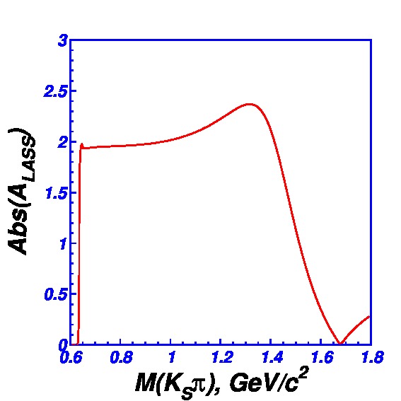
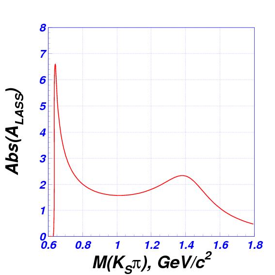
   Figure 2: The absolute value of $F_{S}$ from LASS experiment (left) and from the $\tau^{-}\to K^{0}_{S}\pi^{-}\nu_{\tau}$ study at Belle (right).

   The shape of the optimal scalar form factor in the LASS experiment strongly differs (especially, near the threshold of the $K^{0}_{S}\pi^{-}$ production) from that obtained in the fit of the $K^{0}_{S}\pi^{-}$ mass distribution in the study of $\tau^{-}\to K^{0}_{S}\pi^{-}\nu_{\tau}$ decay at Belle, see Fig. 2. There is large systematic uncertainty in the near $K^{0}_{S}\pi^{-}$ production threshold part of the spectrum due to the large background from the $\tau^{-}\to K^{0}_{S}\pi^{-}K^{0}_{L}\nu_{\tau}$ decay, whose dynamics is not precisely known. In the new study at $B$ factories it will be possible to suppress this background essentially applying special kinematical constraints.

   A fit to the $K^{0}_{S}\pi^{-}$ invariant mass spectrum also provides a high precision measurement of the $K^{\ast}(892)^{-}$ mass and width: $M(K^{\ast}(892)^{-})=(895.47\pm 0.20({\rm stat.})\pm 0.44({\rm syst.})\pm 0.59({\rm mod.}))\ {\rm MeV}/c^{2}$, $\Gamma(K^{\ast}(892)^{-})=(46.2\pm 0.6({\rm stat.})\pm 1.0({\rm syst.})\pm 0.7({\rm mod.}))\ {\rm MeV}$. While our determination of the width is compatible with most of the previous measurements within experimental errors, our mass value, see Fig. 1 (b), is considerably higher than those before and is consistent with the world average value of the neutral $K^{\ast}(892)^{0}$ mass, which is $(896.00\pm 0.25)$ MeV/$c^{2}$ [15].

   The second analysis of the $\tau^{-}\to K^{0}_{S}\pi^{-}\nu_{\tau}$ decay at Belle was based on the data sample with the luminosity integral of ${\cal L}=669$ fb^-1 which comprises 615 million $\tau^{+}\tau^{-}$ events [11]. One inclusive decay mode $\tau^{-}\to K^{0}_{S}X^{-}\nu_{\tau}$ and 6 exclusive hadronic $\tau$ decay modes with $K^{0}_{S}$ ($\tau^{-}\to K^{0}_{S}\pi^{-}\nu_{\tau}$, $\tau^{-}\to K^{0}_{S}K^{-}\nu_{\tau}$, $\tau^{-}\to K^{0}_{S}K^{0}_{S}\pi^{-}\nu_{\tau}$, $\tau^{-}\to K^{0}_{S}\pi^{-}\pi^{0}\nu_{\tau}$, $\tau^{-}\to K^{0}_{S}K^{-}\pi^{0}\nu_{\tau}$, $\tau^{-}\to K^{0}_{S}K^{0}_{S}\pi^{-}\pi^{0}\nu_{\tau}$) were studied in Ref. [11]. In this study signal events were tagged by one-prong tau decays (into $e\nu\nu$, $\mu\nu\nu$ or $\pi/K(n\geq 0)\pi^{0}\nu$ final states) with the branching fraction ${\cal B}_{1-\rm prong}=(85.35\pm 0.07)\%$. In total, $157836$ events of the $\tau^{-}\to K^{0}_{S}\pi^{-}\nu_{\tau}$ decay were selected with the fraction of the non-cross-feed background of $(8.86\pm 0.05)\%$ and the detection efficiency $\varepsilon_{\rm det}=(7.09\pm 0.12)\%$. The obtained branching fraction:

   $${\cal B}(\tau^{-}\to K^{0}_{S}\pi^{-}\nu_{\tau})=(4.16\pm 0.01({\rm stat.})\pm 0.08({\rm syst.})))\times 10^{-3}$$

   supersedes the previous Belle result and has the best accuracy.

   

   

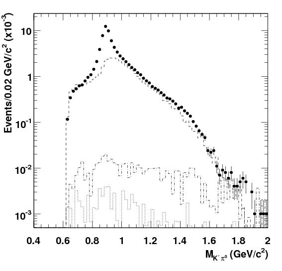
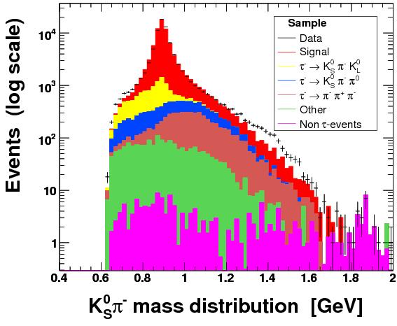
   Figure 3: The $K^{-}\pi^{0}$ invariant mass distribution (left) from Ref. [12]. The dots are experimental data, histograms are background MC events with selection and efficiency corrections: background from $\tau\tau$ (dashed line), $q\bar{q}$ (dash-dotted line), $\mu^{+}\mu^{-}$ (dotted line). The $K^{0}_{S}\pi^{-}$ invariant mass distribution (right) from Ref. [13]. The dots are experimental data, histograms are signal and background MC: signal events (red), dominant background from the $\tau^{-}\to K^{0}_{S}K^{0}_{L}\pi^{-}\nu_{\tau}$ decay (yellow), non-$\tau\tau$ events (magenta).

   Precision measurement of the branching fraction of the $\tau^{-}\to K^{-}\pi^{0}\nu_{\tau}$ decay with a $230.2$ fb^-1 data sample collected at the $\Upsilon(4S)$ resonance has been carried out by BaBar [12]. The result:

   $${\cal B}(\tau^{-}\to K^{-}\pi^{0}\nu_{\tau})=(4.16\pm 0.03({\rm stat.})\pm 0.18({\rm syst.})))\times 10^{-3}$$

   is consistent with the previous measurements and ${\cal B}(\tau^{-}\to K^{0}_{S}\pi^{-}\nu_{\tau})$ and has the best accuracy. The $K^{-}\pi^{0}$ invariant mass distribution is shown in Fig. 3.

   The preliminary result on the ${\cal B}(\tau^{-}\to K^{0}_{S}\pi^{-}\nu_{\tau})$ using a $384.6$ fb^-1 data sample was also published by BaBar [13]:

   $${\cal B}(\tau^{-}\to K^{0}_{S}\pi^{-}\nu_{\tau})=(4.20\pm 0.02({\rm stat.})\pm 0.12({\rm syst.})))\times 10^{-3}.$$

   It is consistent with the other measurements. The distribution of the invariant mass of the $K^{0}_{S}\pi^{-}$ system is shown in Fig. 3, experimental data exhibit additional contribution around the invariant mass of 1.4 GeV/$c^{2}$, which is not included in the signal MC simulation.

3. Search for CPV in $\tau\to K\pi\nu$

   Recent studies of CPV in the $\tau^{-}\to\pi^{-}K_{S}(\geq 0\pi^{0})\nu_{\tau}$ decays at BaBar [14] as well as in the $\tau^{-}\to K_{S}\pi^{-}\nu_{\tau}$ decay at Belle [10] provide complementary information about sources of CPV in these hadronic decays.

   The decay-rate asymmetry $A_{\rm CP}=\frac{\Gamma(\tau^{+}\to\pi^{+}K_{S}(\geq 0\pi^{0})\nu_{\tau})-\Gamma(\tau^{-}\to\pi^{-}K_{S}(\geq 0\pi^{0})\nu_{\tau})}{\Gamma(\tau^{+}\to\pi^{+}K_{S}(\geq 0\pi^{0})\nu_{\tau})+\Gamma(\tau^{-}\to\pi^{-}K_{S}(\geq 0\pi^{0})\nu_{\tau})}$ was studied at BaBar with the $\tau^{+}\tau^{-}$ data sample of $\int Ldt=476$ fb^-1. The obtained result $A_{\rm CP}=(-0.36\pm 0.23\pm 0.11)\%$ is about $2.8$ standard deviations from the SM expectation $A^{K^{0}}_{\rm CP}=(+0.36\pm 0.01)\%$.

   At Belle, CPV search was performed as a blinded analysis based on a $699\leavevmode\nobreak\ {\rm fb}^{-1}$ data sample. Specially constructed asymmetry, which is a difference between the mean values of the $\cos\beta\cos\psi$ for $\tau^{-}$ and $\tau^{+}$ events, was measured in bins of $K^{0}_{S}\pi^{-}$ mass squared ($Q^{2}=M^{2}(K^{0}_{S}\pi)$):

   $$A_{i}^{CP}(Q^{2}_{i})=\frac{\int\limits_{\Delta Q^{2}_{i}}\cos{\beta}\cos{\psi}\left(\frac{d\Gamma_{\tau^{-}}}{d\omega}-\frac{d\Gamma_{\tau^{+}}}{d\omega}\right)d\omega}{\frac{1}{2}\int\limits_{\Delta Q^{2}_{i}}\left(\frac{d\Gamma_{\tau^{-}}}{d\omega}+\frac{d\Gamma_{\tau^{+}}}{d\omega}\right)d\omega}\simeq\langle\cos\beta\cos\psi\rangle_{\tau^{-}}-\langle\cos\beta\cos\psi\rangle_{\tau^{+}},$$

   where $\beta$, $\theta$ and $\psi$ are the angles, evaluated from the measured parameters of the final hadrons, $d\omega=dQ^{2}d\!\cos\theta d\!\cos\beta$. In contrary to the decay-rate asymmetry the introduced $A_{i}^{CP}(Q^{2}_{i})$ is already sensitive to the CPV effects from the charged scalar boson exchange [17]. No CP violation was observed and the upper limit on the CPV parameter $\eta_{S}$ was extracted to be: $|{\rm Im}(\eta_{S})|<0.026$ at 90% CL. Using this limit parameters of the Multi-Higgs-Doublet models [18, 19] can be constrained as $|{\rm Im}(XZ^{\ast})|<0.15\leavevmode\nobreak\ M_{H^{\pm}}^{2}/(1\,\mathrm{GeV}^{2}/c^{4})$, where $M_{H^{\pm}}$ is the mass of the lightest charged Higgs boson, the complex constants Z and X describe the coupling of the Higgs boson to leptons and quarks respectively.

4. Further Studies of $\tau\to K\pi\nu$ Decays

   In the analysis of the $\tau^{-}\to K^{0}_{S}\pi^{-}\nu_{\tau}$ decay, it is very desirable to measure separately vector ($F_{V}$), scalar ($F_{S}$) form factors and their interference. The $K^{\ast}(892)^{-}$ mass and width are measured in the vector form factor taking into account the effect of the interference of the $K^{\ast}(892)^{-}$ amplitude with the contributions from the radial exitations, $K^{\ast}(1410)^{-}$ and $K^{\ast}(1680)^{-}$. The scalar form factor is important to unveil the problem of the $K_{0}^{\ast}(800)^{-}$ state as well as for the tests of the various fenomenological models and search for CPV. The interference between vector and scalar form factors is necessary in the search for CPV in $\tau^{-}\to K^{0}_{S}\pi^{-}\nu_{\tau}$ decay.

   To elucidate the nature of the $K^{\ast}(892)^{-}-K^{\ast}(892)^{0}$ mass difference it is important to study the following modes: $\tau^{-}\to K^{0}_{S}\pi^{-}\nu_{\tau}$, $\tau^{-}\to K^{0}_{S}\pi^{-}\pi^{0}\nu_{\tau}$, $\tau^{-}\to K^{0}_{S}K^{-}\pi^{0}\nu_{\tau}$. $K^{\ast}(892)^{-}$ mass and width can be measured in the clean experimental conditions without disturbance from the final state interactions in the $\tau^{-}\to K^{0}_{S}\pi^{-}\nu_{\tau}$ decay. While a study of the $\tau^{-}\to K^{0}_{S}\pi^{-}\pi^{0}\nu_{\tau}$ mode allows one to measure simultaneously in one mode the $K^{\ast}(892)^{-}$($K^{0}_{S}\pi^{-}$) and the $K^{\ast}(892)^{0}$($K^{0}_{S}\pi^{0}$) masses. The effect of the pure hadronic interaction of the $K^{\ast}(892)^{-}$ ($K^{\ast}(892)^{0}$) and $\pi^{0}$($\pi^{-}$) on the $K^{\ast}(892)^{-}$($K^{\ast}(892)^{0}$) mass can be precisely measured as well. It is also important to investigate precisely the effect of the pure hadronic interaction of the $K^{\ast}(892)^{-}$($K^{\ast}(892)^{0}$) and $K^{0}_{S}$($K^{-}$) on the $K^{\ast}(892)^{-}$($K^{\ast}(892)^{0}$) mass in the $\tau^{-}\to K^{0}_{S}K^{-}\pi^{0}\nu_{\tau}$ decay.

5. Summary

   Belle and BaBar essentially improved the accuracy of the branching fractions of the $\tau^{-}\to(K\pi)^{-}\nu_{\tau}$ decays. At Belle the $K^{0}_{S}\pi$ invariant mass spectrum was studied and the $K^{\ast}(892)^{-}$ alone is not sufficient to describe the $K^{0}_{S}\pi$ mass spectrum. The best description is achieved with the $K_{0}^{\ast}(800)^{-}+K^{\ast}(892)^{-}+K^{\ast}(1410)^{-}$ and $K_{0}^{\ast}(800)^{-}+K^{\ast}(892)^{-}+K_{0}^{\ast}(1430)^{-}$ models. For the first time the the $K^{\ast}(892)^{-}$ mass and width have been measured in $\tau$ decay at $B$ factories. The $K^{\ast}(892)^{-}$ mass is significantly different from the current world average value, it agrees with the $K^{\ast}(892)^{0}$ mass. Precision study of the $\tau^{-}\to K^{0}_{S}\pi^{-}\nu_{\tau}$, $\tau^{-}\to K^{0}_{S}\pi^{-}\pi^{0}\nu_{\tau}$ and $\tau^{-}\to K^{0}_{S}K^{-}\pi^{0}\nu_{\tau}$ decays at the $B$ factories as well as the $e^{+}e^{-}\to K^{0}_{S}K^{\pm}\pi^{\mp}$ reaction at the VEPP-2000 [20, 21] and $K-\pi$ scattering amplitude at the coming GlueX experiment [6] could provide additional valuable information about the $K^{\ast}(892)^{-}$ mass, namely unveil an impact of the hadronic and electromagnetic interactions in the final state.

6. Acknowledgments

   I am grateful to Prof. Igor Strakovsky for inviting me to this very interesting workshop. This work was supported by Russian Foundation for Basic Research (Grant No. 17–02–00897–a).

3.8 From $\pi{K}$ Amplitudes to $\pi{K}$ Form Factors (and Back)

Bachir Moussallam

IPN, Université Paris-Sud 11

91406 Orsay, France

1. Introduction

   Pions and kaons are the lightest hadrons in QCD. The $\pi\pi$ interaction plays an important role in generating stable nuclei. Studying the $\pi\pi$ and the $\pi K$ interactions allows to probe the chiral symmetry aspects of QCD at low energy and the resonance structure at higher energy. Sufficiently precise measurements also associated with theoretical, analyticity properties of QCD have allowed to establish the existence of light, exotic, resonances [1] which had remained elusive for many decades.

   In recent years a considerable amount of data on decays of heavy mesons or leptons into light pseudo-scalar mesons have accumulated. The energy dependencies of these decay amplitudes are essentially controlled by the final-state interactions (FSI) among the light mesons. FSI theory relies on analyticity and the existence of a right-hand cut, in each energy variable, which can be associated with unitarity [2].

   Two-mesons form factors are the simplest functions to which FSI theory can be applied in the sense that they depend on a single variable and that the unitarity cut is the only one. We review below some aspects of the $\pi\pi$ scalar and the $\pi K$ scalar and vector form factors. We will recall, in particular, the experimental properties of the interactions which allow for an application of FSI theory in a much larger energy range than the range of purely elastic scattering. We will also consider the possibility, given sufficiently precise determination of the form factors, to improve the precision of the determination of the light meson amplitudes.

2. The $\pi\pi$ Scalar Form Factors

   $\pi\pi$ scattering is exactly elastic in QCD in the energy range $s\leq 16m^{2}_{\pi}$. However, it has long been known that it can be considered as effectively elastic in a larger range. The two main assumptions which underlie the dispersive construction of the form factors in Ref. [3] is that, in the $S$-wave, this effectively elastic region extends up to the $K\bar{K}$ threshold and that beyond this, there exists an energy region in which two-channel unitarity effectively holds. These assumptions are supported by the experimental measurements of the $\pi\pi$ phase-shifts and inelasticities. For instance Fig. 5a of Ref. [4] showing the inelasticity $\eta_{0}^{0}$ indicates clearly that the $\eta_{0}^{0}$ is driven away from 1 by the $f_{0}(980)$ resonance and the cusp-like shape of the curve suggests that $K\bar{K}$ is the leading inelastic channel, while $4\pi$ or $6\pi$ channels play a negligible role up to 1.4 GeV.

   This can be further probed using experimental measurements of the $\pi\pi\to K\bar{K}$ amplitudes. Indeed, if two-channel unitarity holds then the modulus of this amplitude is simply related to the inelasticity. This is illustrated from fig 1 which shows fits to the inelasticity as deduced from the $\pi\pi\to K\bar{K}$ measurements of Refs. [5, 6] compared with the inelasticity measure in $\pi\pi$. The two experiments are in good agreement in the energy energy region $E\geq 1.2$ GeV and the figure indicates that the two-channel unitarity picture could hold up to $E\simeq 1.6$ GeV.

   

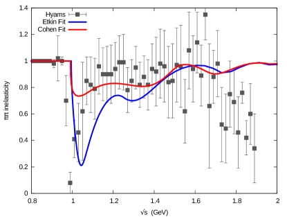
   Figure 1: Inelasticity parameter of the $\pi\pi$ $I=0$ $S$-wave compared to that deduced from $\pi\pi\to K\bar{K}$ measurements assuming two-channel unitarity.

   Scalar form factors, for instance $\Gamma_{\pi}(t)=\langle{\pi(p)\pi(q)|m_{u}\bar{u}u+m_{d}\bar{d}d|0\rangle}$, with $t=(p+q)^{2}$ are analytic functions of $t$ in the whole complex plane except for a right-hand cut on the real axis. Assuming that it has no zeroes, it can be expressed as a phase dispersive representation

   $$\Gamma_{\pi}(t)=\Gamma_{\pi}(0)\exp\left[\frac{t}{\pi}\int_{4{m_{\pi}^{2}}}^{\infty}\frac{dt^{\prime}}{t^{\prime}(t^{\prime}-t)}\,\phi_{\pi}(t^{\prime})\ .\right]$$ (1)

   From Watson’s theorem the form factor phase $\phi_{\pi}$ is equal to the $\pi\pi$ scattering phase in the elastic scattering region, that is, according to the preceding discussion

   $$\phi_{\pi}(t)=\delta_{0}^{0}(t),\ 4{m_{\pi}^{2}}\leq t\leq 4m^{2}_{K}\ .$$ (2)

   Furthermore, when $t\to\infty$ one must have $\phi_{\pi}(t)\to\pi$ which ensures compatibility with a Brodsky-Lepage type behavior [7]. Based on these arguments, a simple interpolating model for the phase in the range $[4m_{K}^{2},\infty]$ was proposed in ref. [8]. As was pointed out in [9] this simple interpolation leads to an overestimate of the pion scalar form factor $\langle r^{2}\rangle^{\pi}_{S}=\dot{\Gamma}_{\pi}(0)/(6\Gamma_{\pi}(0))$ because the $f_{0}(980)$ resonance effect is not properly accounted for. A more accurate interpolation can be performed by exploiting the existence of a two-channel unitarity region and generating the form factor from a solution of the corresponding coupled-channel Muskhelishvili equations

   $$\vec{F}(t)=\frac{1}{\pi}\int_{4{m_{\pi}^{2}}}^{\infty}dt^{\prime}\frac{\bm{T}(t^{\prime})\Sigma(t^{\prime})\vec{F}^{\ast}(t^{\prime})}{t^{\prime}-t},\$$ (3)

   where $\bm{T}$ is the $\pi\pi-K\bar{K}$ coupled-channel matrix and
   $\Sigma(t^{\prime})=diag\left(\sqrt{1-4{m_{\pi}^{2}}/t^{\prime}},\sqrt{1-4m_{K}^{2}/t^{\prime}}\theta(t^{\prime}-4m_{K}^{2})\right)$. Beyond the region where two-channel unitarity applies, a proper asymptotic phase interpolation is performed in this model by imposing asymptotic conditions on the $T$-matrix. It is also convenient to choose these conditions such that the so-called Noether index [10] is equal to ${\cal N}=2$ which ensures that Eq. 3 has a unique solution once two conditions are imposed, e.g., $\Gamma_{\pi}(0)$, $\Gamma_{K}(0)$.

   Fig. 2 illustrates the result for the phase of the form factor, $\phi_{\pi}$, obtained from solving these equations. The $f_{0}(980)$ resonance is predicted to generate a sharp drop in this phase at 1 GeV. Nevertheless, it is noteworthy that the asymptotic phase is reached from above in this approach as is required in QCD [8] (see right plot in Fig. 2). The result for the pion scalar radius [9]: $\langle r^{2}\rangle^{\pi}_{S}=(0.61\pm 0.04)$ $\hbox{fm}^{2}$ is in good agreement with lattice QCD simulations, e.g., [11].

   

   

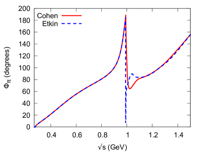
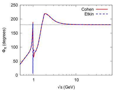
   Figure 2: Phase of the pion scalar form factor from solving the Muskhelishvili equations 3. The right plot illustrates how the asymptotic value is reached.

3. $\pi K$ Scalar Form Factor

   $\pi K$ scattering in the $S$-wave is exactly elastic in QCD in the region $t\leq(m_{K}+3m_{\pi})^{2}$. By analogy with $\pi\pi$ one would expect the amplitude to be effectively elastic in a substantially larger range. This seems to be confirmed by experiment. Fig. 3 shows the inelasticity parameter $\eta_{0}^{1/2}$ obtained from a fit to the two most recent amplitudes determinations [12, 13]. One sees that $\eta_{0}^{1/2}$ remains close to 1 up to $\sqrt{t}\simeq 1.9$ GeV and it is driven away from 1 very sharply by the $K^{\ast}_{0}(1950)$ resonance. The detailed properties of this resonance are yet unknown. It is often assumed that its main decay channel is $\eta^{\prime}K$ which would imply the existence of a two-channel unitarity region for the $\pi K$ $S$-wave. A dispersive derivation of the $\pi K$ scalar form factor exactly analogous to that of $\pi\pi$ can then be performed [14].

   An important difference with $\pi\pi$, though, is that the $\pi K$ scalar form factor is measurable. It can be determined from semi-leptonic decay amplitudes $K\to\pi l\nu_{l}$ and $\tau\to K\pi\nu_{\tau}$ since the matrix element of the vector current involves both the vector and the scalar form factors, $f_{+}^{K\pi}$, $f_{0}^{K\pi}$

   $$\sqrt{2}\langle K^{+}(p_{K})|\bar{u}\gamma^{\mu}{s}|\pi^{0}(p_{\pi})\rangle=f_{+}^{K\pi}(t)\,\left(p_{K}+p_{\pi}-\frac{\Delta_{K\pi}}{t}(p_{K}-p_{\pi})\right)^{\mu}+f_{0}^{K\pi}(t)\,\frac{\Delta_{K\pi}}{t}\left(p_{K}-p_{\pi}\right)^{\mu}$$ (4)

   The prediction from the two-channel dispersive form factor model for the slope parameter $\lambda_{0}=m_{\pi^{+}}^{2}\dot{f}_{0}^{K\pi}(0)/f_{0}^{K\pi}(0)$ is [15] $\lambda_{0}=(14.7\pm 0.4)\cdot 10^{-3}$ which is in rather good agreement with the most recent determination by NA48/2, NA62 experiments [16]: $\lambda_{0}=(14.90\pm 0.55\pm 0.80)\cdot 10^{-3}$. Further verifications of this form factor, in particular in the region of the $K^{\ast}_{0}(1430)$ resonance, would be necessary. This is possible, in principle, from $\tau\to K\pi\nu_{\tau}$ decays if one measures both the energy and the angular distributions in order to disentangle the contributions from the two form factors. At low energy $f_{0}^{K\pi}(t)$ displays a strong $\kappa$ meson induced enhancement. As can be seem from fig. 4 (left plot) below, this feature is in accord with the data already existing on $\tau$ decay.

4. $\pi K$ Vector Form Factor and $J=1$ Amplitude

   For the $P$-wave amplitude, fits to the experimental data indicate that the quasi-elastic range extends up to the $K^{\ast}\pi$ threshold (see fig. 3). The inelasticity is driven by the $K^{\ast}(1410)$ and by the $K^{\ast}(1680)$ resonance. The decay properties of these two resonances have been studied in detail in Ref. [17]: they essentially involve the two quasi two-body channels $K^{\ast}\pi$ and $K\rho$. This suggests that a plausible model based on three-channel unitarity can be developed for describing the $\pi K$ $P$-wave scattering which can be applied to the dispersive construction of the vector form factor. Models of this type were considered [18, 19]. We present below slightly updated results from [18].

   

   

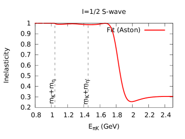
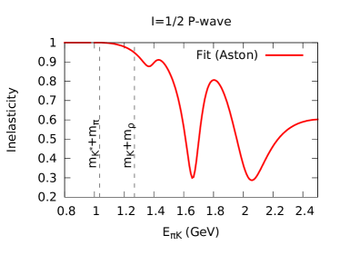
   Figure 3: $\pi K$ inelasticity from fits to the data of [12, 13]. Left plot: $S$-wave, right plot: $P$-wave.

   At first, a reasonable fit of the experimental data can be achieved (with a $\chi^{2}/{d.o.f}=1.8$) in the whole energy range $0.8\leq E\leq 2.5$ GeV within a model which implements exact three-channel unitarity via a simple standard $K$-matrix approach,

   $$K_{ij}=\sum_{R}\frac{g_{R}^{i}\,g_{R}^{j}}{m_{R}^{2}-s}+K_{ij}^{back}\ .$$ (5)

   The model has four $P$-wave resonances and contains 15 parameters which are determined from a fit to the $\pi K\to\pi K$ experimental data. The parameters are also constrained with respect to the inelastic channels $K^{\ast}\pi$ and $K\rho$ by the measured branching fractions of the $K^{\ast}(1410)$, $K^{\ast}(1680)$ resonances.

   The three vector form factors associated with $K\pi$, $K^{\ast}\pi$, $K\rho$ can then be determined by solving the coupled integral dispersive equations analogous to eq. 3. Having chosen ${\cal N}=3$ for the Noether index, it is necessary to provide three constraints in order to uniquely specify the solution, e.g. the values of the three form factors $H_{i}$ at $t=0$. The value of $H_{1}(0)=f_{+}^{K\pi}(0)$ is rather precisely known from chiral symmetry and from lattice QCD simulations (see [20]). Concerning $H_{2}(0)$, $H_{3}(0)$ we can only obtain a qualitative order of magnitude in the limit of exact three-flavor chiral symmetry and assuming exact vector-meson dominance. This gives

   $$H_{2}(0)=-H_{3}(0)=\frac{\sqrt{2}N_{c}M_{V}}{16\pi^{2}F_{V}F_{\pi}}\simeq 1.50\ \hbox{GeV}^{-1}$$ (6)

   We can thus parametrize the exact values as $H_{2}(0)=1.50(1+a)$, $H_{3}(0)=1.50(1+b)$ and we expect $|{a}|,|{b}|<30\%$. Fitting the Belle data [21] on $\tau\to K\pi\nu_{\tau}$ with these two parameters $a$, $b$ gives a rather poor $\chi^{2}=8.6$. While this could simply be blamed on the inadequacy of the model, we will argue instead that the $P$-wave phase-shifts of LASS [17] may need some updating. At first, one sees that much of the large $\chi^{2}$ value originates from the $K^{\ast}(892)$ resonance region and simply reflects a significant difference in the $K^{\ast}(892)$ resonance width between the LASS data and the Belle data. Indeed, in the recent re-analysis of the LASS data constrained by dispersions relations [22] a value for the width, $\Gamma_{K^{\ast}}=58\pm 2$ MeV is found, which is much larger than the result of Belle: $\Gamma_{K^{\ast}}=46.2\pm 1.4$ MeV.

   In the present approach one can go further and determine how the $P$-wave results from LASS need to be modified in order for the vector form factor to be in better agreement with the Belle results. This is done by refitting the parameters of the three-channel $T$ matrix including both LASS and Belle data sets. Doing this, a reasonable agreement with the $\tau$ data can be achieved with a $\chi^{2}/N({Belle})=2.4$ while the $\chi^{2}$ for the LASS data is $\chi^{2}/N({LASS})=3.5$. This is illustrated in fig. 4. The left plot shows the $\pi K$ energy distribution in the $\tau\to\pi K\nu_{\tau}$ mode and the right plot shows the phase of the $\pi^{+}K^{-}\to\pi^{+}K^{-}$ $J=1$ amplitude as a function of energy. Beyond the region of the $K^{\ast}(892)$ a visible modification of the phase in the region of the $K^{\ast}(1410)$ seems to be also needed.

   

   

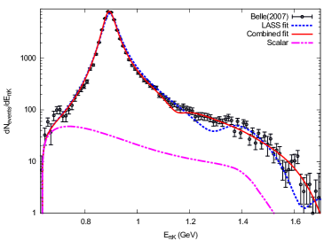
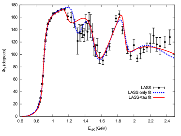
   Figure 4: Left plot: energy distribution in the $\tau\to\pi K\nu_{\tau}$ mode. Right plot: Phase of the $\pi^{+}K^{-}\to\pi^{+}K^{-}$ $J=1$ amplitude. The dashed blue curves show the results when the $T$-matrix parameters are fitted to the LASS data only, while the solid red curves when the fit includes both LASS and Belle data. The dash-dot magenta curve shows the contribution associated with the scalar form factor.

3.9 Three-Body Interaction in Unitary Isobar Formalism

Maxim Mai

Institute for Nuclear Studies and

Department of Physics

The George Washington University

Washington, DC 20052, U.S.A.

1. Introduction

   Interest in the description of three-hadron systems has re-sparked in recent years due to two aspects of modern nuclear physics. First, there are substantial advances of experimental facilities such as COMPASS [1], GlueX [2] and CLAS12 [3] experiments, aiming for the study of meson resonances with mass above 1 GeV including light hybrids. The large branching ratio of such resonances to three pions is expected to generate important features via the final state interaction. Furthermore, effects such as the log-like behavior of the irreducible three-body interaction, associated with the $a_{1}(1420)$ [4] can be studied in detail with a full three-body amplitude. Similarly, the study of the $XYZ$ sector [5, 6] currently explored by LHCb, BESIII, Belle and BaBar [7, 8] can be conducted in more detal when the three-body interactions are taken into account. The prominent Roper puzzle can be re-addressed when the features of the $\pi\pi N$ amplitude are sufficiently under control, see, e.g., Ref. [9]. Finally, the proposed Klong beam experiment at JLab [10, 11, 12, 13] can give new insights into properties of, e.g., $\kappa$-resonance from the $K\pi\pi$ channel. Second, the algorithmic and computational advances in ab-intio Lattice QCD calculations make the analysis of such interesting systems as the Roper-resonance ($N(1440)1/2^{+}$) or the $a_{1}(1260)$ possible. Some first studies in these systems have already been conducted, using gauge configurations with unphysically heavy quark masses [14, 15, 16], but no 3-body operators have been included there yet. Many other groups are working on conducting similar studies, such as, e.g., the $\pi\rho$ scattering in the $I=2$ sector [17]. Also in these systems the pion mass is very heavy, such that the $\rho$ is stable and the infinite-volume extrapolation can effectively be carried out using the two-body Lüscher formalism. In the future, it has to be expected that these and similar studies will be carried out at lower pion masses with an unstable $\rho$ decaying into two pions. For these cases the full understanding of the infinite volume extrapolations including three-body dynamics is desired. Important progress has been achieved in the last years [18, 19, 20, 21, 22, 23, 24, 25, 26, 27, 28, 29, 30], and first numerical case studies have now been conducted with three different approaches [31, 32, 30, 19]. While still exploratory, they mark an important step in the development of the three-body quantization condition.

   In this work, we show theoretical developments of one of these approaches [30] as well as numerical studies based on it. This framework is based on the general formulation of the infinite volume three-to-three scattering amplitude which respects two- and three-body unitarity. At its core, the two-body sub-amplitudes are parametrized by a tower of functions of invariant mass with correct right-hand singularities of the corresponding partial-waves. The truncation of such a series of functions in a practical calculations is the only approximation of such an approach and takes account of the sparsity of the lattice data. The imaginary parts of such an amplitude are fixed by unitarity, giving rise to a power-law (in $ML$ – a dimensionless product of pion mass and size of cubic lattice volume) finite volume dependence, when replacing continuous momenta in such an amplitude by discretized ones due to boundary conditions imposed in Lattice QCD studies. Therefore, such a framework gives a natural way to study three-body systems in the infinite and in finite volume simultaneously.

2. Three-Body Scattering in the Infinite Volume

   

   Figure 1: Total scattering amplitude $\hat{T}$ consisting of a connected ($\hat{T}_{c}$) and a disconnected contribution ($\hat{T}_{d}$), represented by the first and second term on the right-hand side of Eq. (1), respectively. Single lines indicate the elementary particle, double lines represent the isobar, empty dots stand for isobar dissociation vertex $v$, while time runs from right to left. $T$ and $"+"$ denote the isobar-spectator scattering amplitude and isobar propagator $\tau$, respectively.

   The interaction of three-to-three asymptotic states is described by the scattering amplitude $T$. We assume here that the particles in question are stable, spinless and identical (of mass $M$) for simplicity. The connectedness-structure of matrix elements dictates that the scattering amplitude consists of two parts: the fully connected one and one-time disconnected, denoted by the subscript $c$ and $d$ in the following. As discussed in Refs. [33, 19], the full two-body amplitude can be re-parametrized by a tower of “isobars", which for given quantum numbers of the two-body sub-system describe the correct right-hand singularities of each partial wave in that system. In this sense the isobar formulation is not an approximation but a re-parametrization of the full two-body amplitude, see the discussion in the original work [34]. In summary, the three-to-three scattering amplitude (depicted in Fig. 1) reads

   $$\langle q_{1},q_{2},q_{3} |\hat{T}|p_{1},p_{2},p_{3}\rangle=\langle q_{1},q_{2},q_{3}|\hat{T}_{c}|p_{1},p_{2},p_{3}\rangle+\langle q_{1},q_{2},q_{3}|\hat{T}_{d}|p_{1},p_{2},p_{3}\rangle$$ (1)

   $$=\frac{1}{3!}\sum_{n=1}^{3}\sum_{m=1}^{3}\,v(q_{\bar{n}},q_{\bar{\bar{n}}})v(p_{\bar{m}},p_{\bar{\bar{m}}})$$

   $$\leavevmode\nobreak\ \leavevmode\nobreak\ \leavevmode\nobreak\ \leavevmode\nobreak\ \leavevmode\nobreak\ \leavevmode\nobreak\ \leavevmode\nobreak\ \leavevmode\nobreak\ \leavevmode\nobreak\ \leavevmode\nobreak\ \leavevmode\nobreak\ \Bigg{(}\tau(\sigma(q_{n}))\,T(q_{n},p_{m};s)\,\tau(\sigma(p_{m}))\,-2E({\bm{q}}_{n})\tau(\sigma(q_{n}))(2\pi)^{3}\delta^{3}(\bm{q}_{n}-\bm{p}_{m})\Bigg{)}\,,$$

   where $P$ is the total four-momentum of the system, $s=W^{2}=P^{2}$ and $E({\bm{p}})=\sqrt{{\bm{p}}^{2}+M^{2}}$. All four-momenta $p_{1},q_{1},...$ are on-mass-shell, and the square of the invariant mass of the isobar reads $\sigma(q):=(P-q)^{2}=s+M^{2}-2WE(\bm{q})$ for the spectator momentum $q$. We work in the total center-of-mass frame where ${\bm{P}}=\bm{0}$ and denote throughout the manuscript three-momenta by bold symbols. The dissociation vertex $v(p,q)$ of the isobar decaying in asymptotically stable particles, e.g., $\rho\,(p+q)\to\pi(p)\pi(q)$, is chosen to be cut-free in the relevant energy region, which is always possible. The notation is such that, e.g., for a spectator momentum $q_{n}$ the isobar decays into two particles with momenta $q_{\bar{n}}$ and $q_{\bar{\bar{n}}}$. Finally, $T$ describes the isobar-spectator interaction and is the function of eight kinematic variables allowed by momentum and energy conservation, such as the full three-to-three scattering amplitude.

   The above equation contains three unknown functions $\tau(\sigma)$, $T$ and $v$. Since real and imaginary parts of the scattering amplitude are related by unitarity, the latter building blocks of the scattering amplitude are related between each other as well. Specifically, including a complete set of three-particle intermediate states (inclusion of higher-particle states will be studied in a future work) the three-body unitarity condition can be written as

   $$\langle q_{1},q_{2},q_{3}|(\hat{T}-\hat{T}^{\dagger})| p_{1},p_{2},p_{3}\rangle=$$ (2)

   $$i\int\prod_{\ell=1}^{3}\frac{\mathrm{d}^{4}k_{\ell}}{(2\pi)^{4}}\,(2\pi)\delta^{+}(k_{\ell}^{2}-m^{2})\,(2\pi)^{4}\delta^{4}\left(P-\sum_{\ell=1}^{3}\,k_{\ell}\right)$$

   $$\leavevmode\nobreak\ \leavevmode\nobreak\ \leavevmode\nobreak\ \leavevmode\nobreak\ \leavevmode\nobreak\ \leavevmode\nobreak\ \leavevmode\nobreak\ \leavevmode\nobreak\ \leavevmode\nobreak\ \leavevmode\nobreak\ \leavevmode\nobreak\ \leavevmode\nobreak\ \leavevmode\nobreak\ \leavevmode\nobreak\ \leavevmode\nobreak\ \leavevmode\nobreak\ \leavevmode\nobreak\ \leavevmode\nobreak\ \leavevmode\nobreak\ \leavevmode\nobreak\ \leavevmode\nobreak\ \leavevmode\nobreak\ \langle q_{1},q_{2},q_{3}|\hat{T}^{\dagger}|k_{1},k_{2},k_{3}\rangle\,\langle k_{1},k_{2},k_{3}|\hat{T}|p_{1},p_{2},p_{3}\rangle\,,$$

   where $\delta^{+}(k^{2}-m^{2}):=\theta(k_{0})\delta(k^{2}-m^{2})$. To reveal the relations between $T$, $\tau$ and $v$ we make the Bethe-Salpeter Ansatz for the isobar-spectator amplitude

   $$T(q_{n},p_{m};s)=B(q_{n},p_{m};s)+\int\frac{\mathrm{d}^{4}k}{(2\pi)^{4}}B(q_{n},k;s)\hat{\tau}(\sigma(k))T(k,p_{m};s)\,,$$ (3)

   which holds for any in/outgoing spectator momenta $p_{m}/q_{n}$ (not necessarily on-shell), and effectively re-formulates the unknown function $T$ by yet another two unknown functions: the isobar-spectator interaction kernel $B$ and the isobar-spectator Green’s function $\hat{\tau}$. In particular, we can rewrite the left-hand-side of the unitarity relation (2) into eight different topologies, which symbolically read

   $$\hat{T}-\hat{T}^{\dagger}= \leavevmode\nobreak\ v(\tau-\tau^{\dagger})v+v\left(\tau-\tau^{\dagger}\right)T\tau v+v\tau^{\dagger}T^{\dagger}\left(\tau-\tau^{\dagger}\right)v$$

   $$+v\tau^{\dagger}(B-B^{\dagger})\tau v+v\tau^{\dagger}(B-B^{\dagger})\hat{\tau}T\tau v+v\tau^{\dagger}T^{\dagger}\hat{\tau}^{\dagger}(B-B^{\dagger})\tau v$$ (4)

   $$+v\tau^{\dagger}T^{\dagger}(\hat{\tau}-\hat{\tau}^{\dagger})T\tau v+v\tau^{\dagger}T^{\dagger}\hat{\tau}^{\dagger}(B-B^{\dagger})\hat{\tau}T\tau v\,.$$

   The main goal of such a decomposition is to express the discontinuity of $\hat{T}$ as a sum of discontinuities of simpler building blocks in corresponding variables.

   The same kind of decomposition can be achieved for the right-hand-side of unitarity relation (2), inserting $\hat{T}=\hat{T}_{d}+\hat{T}_{c}$ there, while keeping in mind the permutations of particle indices as in Eq. (1). The exact formulation of this is discussed in detail in the original publication [34]. Here we restrict ourselves of mentioning that piecewise comparison of all structures to those of Eq. (2) leads to eight independent matching relations. These can be fulfilled simultaneously imposing

   $$\hat{\tau}(\sigma(k)) = \leavevmode\nobreak\ -(2\pi)\delta^{+}(k^{2}-m^{2})\tau(\sigma(k))\,,$$ (5)

   $$B(q,p;s)-B^{\dagger}(q,p;s) = \leavevmode\nobreak\ iv(Q,q)(2\pi)\delta^{+}(Q^{2}-m^{2})v(Q,p)\,,$$ (6)

   $$\Big{(}\tau^{\dagger}(\sigma(k))\Big{)}^{-1}-\Big{(}\tau(\sigma(k))\Big{)}^{-1} = \leavevmode\nobreak\ i\int\frac{\mathrm{d}^{4}\bar{K}}{2(2\pi)^{2}}\,\delta^{+}\left(\left(\tilde{P}+\bar{K}\right)^{2}-m^{2}\right)\delta^{+}\left(\left(\tilde{P}-\bar{K}\right)^{2}-m^{2}\right)$$ (7)

   $$\leavevmode\nobreak\ \leavevmode\nobreak\ \leavevmode\nobreak\ \leavevmode\nobreak\ \leavevmode\nobreak\ \leavevmode\nobreak\ \leavevmode\nobreak\ \leavevmode\nobreak\ \leavevmode\nobreak\ \leavevmode\nobreak\ \leavevmode\nobreak\ \leavevmode\nobreak\ \leavevmode\nobreak\ \leavevmode\nobreak\ \leavevmode\nobreak\ \left(v\left(\tilde{P}+\bar{K},\tilde{P}-\bar{K}\right)\right)^{2}\,,$$

   where $\tilde{P}:=(P-k)/2$ and $Q:=P-p-q$. The direct consequence of the above relations is that the number of unknown in the integral equation defining the three-to-three scattering amplitude (1) is naturally reduced from three ($\hat{\tau}$, $B$, $\tau$) to two ($\tau$, $B$). The remaining two can be determined using twice subtracted dispersion relation w.r.t the invariant mass of the two-body system ($\sigma$) as well an un-subtracted dispersion relation in $Q^{2}$, respectively. The exact integral representation of $B$ and $\tau$ is given in the original publication [34] and resembles the one-particle exchange as well as a fully dressed isobar propagator. In both cases a real-valued function can be added, without altering the discontinuity relations and, thus, being allowed by the unitarity constraint discussed here.

   The above considerations finalize the form of the three-to-three scattering amplitude as demanded by three-body unitarity and compositeness principle. It is a fully relativistic three-dimensional integral equation, which becomes a coupled-channel equation when more than one isobar is considered for the parametrization of the two-to-two scattering. The parameters of these isobars (subtraction constants) can be fixed from the two-body scattering data, while the real part of $B(q,p;s)$ has to be fixed from the three-body data. The application of this approach to systems like the $a_{1}(1260)$ with two isobars, i.e., isovector and isoscalar $\pi\pi$ channels, is work in progress.

3. Three-Body Scattering in Finite Volume

   

   

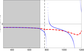
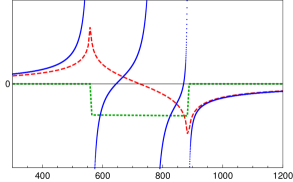
   Figure 2: Left: isobar propagator $\tau$ in the finite volume (blue line) and the real part of the infinite volume one (red dashed line) for a given boost $\bm{l}=(0,0,2\pi/L)$ and $L=3.5$ fm. The gray dashed line denotes the onshell-condition of two particles ($\sigma(\bm{l})=(2M)^{2}$), whereas the gray area represents the energy range for which $\sigma(\bm{l})\leq 0$. Right: Red dashed line (green dotted line) represent real (imaginary) part of the infinite-volume $S$-wave projection of the isobar-spectator interaction kernel $B$. In comparison, the finite-volume projection $B^{A_{1}^{+}}$ for the transition from shell 1 to shell 1 at $L=6$ fm (blue dots).

   As discussed in the introduction, one of the main goals for the present investigations on the unitarity constraints on three-body systems is the derivation of the finite-volume spectrum in such systems. To re-iterate, the main idea is that unitarity fixes the imaginary parts of the amplitude, which themselves lead to the power-law dependence of finite-volume corrections.

   To begin, we note that since $v$ (the isobar dissociation vertex into asymptotically stable particles) is a cut-free function in momenta, it will not lead to any power-law finite-volume effects. Thus, the desired quantization condition will be entirely derived from the part in brackets of the second line of Eq. (1). The non-trivial part of this expression is the isobar-spectator scattering amplitude $T$, which in integral form reads

   $$T(q,p;s)=B(q,p;s)-\int\frac{\mathrm{d}^{3}\bm{l}}{(2\pi)^{3}}B(q,l;s)\frac{\tau(\sigma(l))}{2E({\bm{l}})}T(l,p;s)\,,$$ (8)

   where the parameters of the isobar-propagator $\tau$ can be fixed from two-body scattering data, defining the two-to-two scattering amplitude via $T_{22}:=v\tau v$.

   In the finite cubic volume with periodic boundary conditions the momenta are discretized. In particular, in a cube of a size $L$ only the following three-momenta are allowed (organized by “shells”)

   $${\bm{q}}_{ni}=\frac{2\pi}{L}\,{\bm{r}}_{i}\text{\leavevmode\nobreak\ for\leavevmode\nobreak\ }\{{\bm{r}}_{i}\in\mathds{Z}^{3}|{\bm{r}}_{i}^{2}=n,i=1,\dots,\vartheta(n)\}\ .$$ (9)

   where $\vartheta(n)=1,6,12,\dots$ indicates the multiplicity (number of points in shell $n=0,1,2,\dots$) that can be calculated as described, e.g., in Refs. [35, 32]. In principle, replacing all momenta in Eqs. (1, 8, 12) including the replacement of the appearing integrals over solid angle as ${\int d\Omega_{\bm{p}_{n}}\to\frac{4\pi}{\vartheta(n)}\sum_{i=1}^{\vartheta(n)}}$ leads to a generic three-body quantization condition – an equation which determines the positions of singularities of such an amplitude in energy. However, several subtleties arise from the breakdown of the spherical symmetry on the lattice, which we wish to discuss in the following.

   First of all, the isobar propagator in the second line of Eq. (12) is evaluated in the isobar center-of-mass frame. In the finite volume, however, the allowed momenta given by Eq. (9) are defined in the three-body rest frame at $\bm{P}=\bm{0}$. For the calculation of the finite-volume self-energy one, therefore, has to boost the momenta to the isobar rest frame. In this context it is important to recall that the two-body sub-system can become singular when the invariant mass of the system becomes real, see, e.g., Fig. 2. The tower (for all spectator momenta in question) of two-body singularities has to cancel such that only genuine three-body singularities remain in the final expression. As it is shown analytically in the original publication [30], such cancellation occur in the full quantization condition when all terms (including disconnected topology $\hat{T}_{d}$) and boosts are taken into account accordingly.

   Another important observation w.r.t the breakdown of spherical symmetry is that the isobar-spectator interaction kernel is singular for specific combination of momenta and energies. Expressed differently, when projecting to a partial wave in infinite volume, this term develops an imaginary part below threshold as presented for the S-wave projection of $B$ in Fig. 2. Thus, in finite volume the same term has to have a series of singularities in this region. This indeed happens when projecting $B$ to the corresponding irreducible representation ($A_{1}^{+}$ for the depicted case) of the cubic symmetry group $O_{h}$. Furthermore, the projection to irreps of $O_{h}$ of the three-body scattering amplitude has two additional advantages. For once, the results of Lattice QCD calculation are usually projected to these irreps. Additionally, the projection to different irreps reduces the dimensionality of the three-body scattering amplitude and therefore also that of the quantization condition in the finite volume.

   There are various ways of projecting to definite irreps in the finite volume. In Ref. [32] a method has been developed, which has a form very similar to the usual partial-wave projection in infinite volume. We refer the reader for more details on the construction techniques of this method to the original publication [32], and quote here only the corresponding result. A given function $f^{s}(\bf\hat{p}_{j})$ acting on momenta of the shell $s$ can be expanded as

   $$f^{s}({\bf\hat{p}}_{j})=\sqrt{4\pi}\sum_{\Gamma\alpha}\sum_{u}f^{\Gamma\alpha s}_{u}\chi_{u}^{\Gamma\alpha s}({\bf\hat{p}}_{j})\,\text{\leavevmode\nobreak\ \leavevmode\nobreak\ for\leavevmode\nobreak\ \leavevmode\nobreak\ }f^{\Gamma\alpha s}_{u} =\frac{\sqrt{4\pi}}{\vartheta(s)}\,\sum_{j=1}^{\vartheta(s)}f^{s}({\bf\hat{p}}_{j})\chi^{\Gamma\alpha s}_{u}({\bf\hat{p}}_{j})\,,$$ (10)

   where $\Gamma$, $\alpha$, and $u$ denote the irrep, basis vector of the irrep and the corresponding index, respectively. In these indices the functions $\chi_{u}^{\Gamma\alpha s}$ build an orthonormal basis of functions acting on momenta on the shell $s$.

   Using the projection method presented above our final result for three-body quantization condition for the irrep $\Gamma$ reads

   $${\rm Det}\left[B^{\Gamma ss^{\prime}}_{uu^{\prime}}(W^{2})+\frac{2E_{s}\,L^{3}}{\vartheta(s)}\tau_{s}(W^{2})^{-1}\delta_{ss^{\prime}}\delta_{uu^{\prime}}\right]=0\,,$$ (11)

   where $W$ is the total energy of three-body system, $E_{s}=\sqrt{{\bf p}_{i}^{2}+M^{2}}$ and $\tau_{s}(W^{2}):=\tau(\sigma(p_{i}))$ for any three-momentum on the shell $s$. Note that the determinant is taken with respect to a matrix in shell-indices ($s,s^{\prime}$), as well as basis indices $(u,u^{\prime})$ of the functional basis to the irrep $\Gamma$, whereas the dependence on $\alpha$ drops off naturally. To demonstrate the usefulness of the derived quantization condition we fix $m=139$ MeV and $L=3.5$ fm. Furthermore, we assume one S-wave isobar with $v(p,q):=\lambda f((p-q)^{2})$ with $f$ such that it is 1 for $(p-q)^{2}=0$ and decreases sufficiently fast for large momentum difference, e.g., $f(Q^{2})=\beta^{2}/(\beta^{2}+Q^{2})$ to regularize integrals of the scattering equation. Note that one is not obliged to use form factors but can instead formulate the dispersive amplitude through multiple subtractions rendering it automatically convergent, see Eq. (14) in Ref. [34]. This leads to

   $$B(q,p;s)= \frac{-\lambda^{2}f((P-q-2p)^{2})f((P-2q-p)^{2})}{2E({\bm{q}}+{\bm{p}})\left(W-E({\bm{q}})-E({\bm{p}})-E({\bm{q}}+{\bm{p}})+i\epsilon\right)}+C(q,p;s)\,,$$ (12)

   $$\frac{1}{\tau(\sigma(l))}= \sigma(l)-M_{0}^{2}-\int\frac{d^{3}\bm{k}}{(2\pi)^{3}}\frac{\lambda^{2}(f(4\bm{k}^{2}))^{2}}{2E({\bm{k}})(\sigma(l)-4E({\bm{k}})^{2}+i\epsilon)}\,,$$

   where $C$ is a real-valued function of total energy and both spectator momenta, while $M_{0}$ is a free parameter that is fixed (together with $\lambda$ and $\beta$) to reproduce some realistic two-body scattering data. In the present case we take the experimental phase-shifts for the $\pi\pi$ scattering in the isovector channel for demonstration, and fix $C=0$ and $\Gamma=A_{1}^{+}$ for simplicity.

   

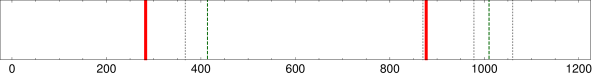
   Figure 3: The red lines show finite-volume energy eigenvalues for $L=3.5$ fm and $M=139$ MeV. The doted gray vertical lines show the positions of singularities of $\tau$ for all used boost momenta, while the dashed green vertical lines show the position of non-interacting energy eigenvalues of three particles.

   The result of the numerical investigation is depicted in Fig. 3. It shows the non-interacting levels of the three-body system (green, dashed lines) along with the solutions of the quantization condition (11) (full, red lines) representing the interacting energy eigenvalues. Since $\chi^{A_{1}^{+}}=1/\sqrt{4\pi}$ the dimensionality of the matrix is given entirely by the set of considered shells. We have checked that using more than 8 first shells does not lead to visible change of the position of the interacting levels. Constraining ourselves to these shells is equivalent to a momentum cutoff of $\sim 1$ GeV for the given lattice volume. Note also that the range of applicability of the quantization condition is, in principle, also restricted by construction, due to missing intermediate higher-particle states. The later is common to all present studies of the three-body in finite volume, and has to be eased at some point in future. However, this study demonstrates clearly the usefulness and practical applicability of the derived quantization condition. Further studies, such as volume dependence and inclusion of multiple isobars are work in progress.

4. Acknowledgments

   The speaker thanks the organizers of the workshop for the invitation and productive discussions during the workshop. Furthermore, he is grateful for the financial support by the German Research Foundation (DFG), under the fellowship MA 7156/1-1, as well as for the George Washington University for the hospitality and inspiring environment.

3.10 Study of the Processes $e^{+}e^{-}\to K\bar{K}n\pi$ with the CMD-3 Detector at VEPP-2000 Collider

Vyacheslav Ivanov (on behalf of CMD-3 Collaboration)

Budker Institute of Nuclear Physics

Novosibirsk, 630090 Russia

1. Introduction

   A high-precision measurement of the inclusive $e^{+}e^{-}{\to}\leavevmode\nobreak\ hadrons$ cross section is required for a calculation of the hadronic contribution to the muon anomalous magnetic moment $(g-2)_{\mu}$ in the frame of the Standard Model. To confirm or deny the observed difference between the calculated $(g-2)_{\mu}$ value [1] and the measured one [2], more precise measurements of the exclusive channels of $e^{+}e^{-}{\to}\leavevmode\nobreak\ hadrons$ are necessary. The exclusive $KK(n)\pi$ final states are of special interest, since their producltion involves rich intermediate dynamics which allows the test of isotopic relations and measurement of intermediate vector mesons parameters.

   In this paper we describe the current status of the study of $e^{+}e^{-}{\to}K^{+}K^{-}\pi^{+}\pi^{-}$, $K^{+}K^{-}\eta$, $K^{+}K^{-}\omega(782)$ and $K^{+}K^{-}\pi^{0}$ processes with the CMD-3 detector at VEPP-2000 collider (Novosibirsk, Russia), based on about $20$ pb^-1 of data, collected in the runs of 2011-2012 years, and about $50$ pb^-1 in the runs of 2017 year. The preliminary results for $\phi(1680)$ meson parameters were obtained from $K^{+}K^{-}\eta$ cross section fitting. We see also the indication on non trivial behavior of $e^{+}e^{-}{\to}K^{+}K^{-}\pi^{+}\pi^{-}$ process cross section at $p\bar{p}$ threshold.

2. VEPP-2000 collider and CMD-3 detector

   The VEPP-2000 $e^{+}e^{-}$ collider [3] at Budker Institute of Nuclear Physics covers the $E_{\rm c.m.}$ range from 0.32 to 2.0 GeV and employs a technique of round beams to reach luminosity up to 10³² cm^-2s^-1 at $E_{\rm c.m.}$=2.0 GeV. The Cryogenic Magnetic Detector (CMD-3) described in [4] is installed in one of the two beam interaction regions. The tracking system of the CMD-3 detector consists of a cylindrical drift chamber (DC) and a double-layer cylindrical multiwire proportional Z-chamber, installed inside a superconducting solenoid with a 1.0–1.3 T magnetic field (see CMD-3 layout in Fig. 1). Amplitude information from the DC wires is used to measure the specific ionization losses ($dE/dx_{\rm DC}$) of charged particles. Bismuth germanate crystals of 13.4 $\rm X_{0}$ thickness are used in the endcap calorimeter. The barrel calorimeter, placed outside the solenoid, consists of two parts: internal (based on liquid Xenon (LXe) of 5.4 $\rm X_{0}$ thickness) and external (based on CsI crystals of 8.1 $\rm X_{0}$ thickness) [5].

   

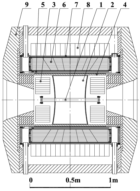
   Figure 1: The CMD-3 detector layout: 1 - beam pipe, 2 - drift chamber, 3 - BGO endcap calorimeter, 4 - Z-chamber, 5 - superconducting solenoid, 6 - LXe calorimeter, 7 - time-of-flight system, 8 - CsI calorimeter, 9 - yoke.

   The physics program of CMD-3 includes:

   • precise measurement of the $R=\sigma(e^{+}e^{-}{\to}hadrons)/\sigma(e^{+}e^{-}{\to}\mu^{+}\mu^{-})$, neccessary for clarification of $(g-2)_{\mu}$ puzzle;

   • study of the exclusive hadronic channels of $e^{+}e^{-}$ annihilation, test of isotopic relations;

   • study of the $\rho$, $\omega$, $\phi$ vector mesons and their excitations;

   • CVC tests: comparison of isovector part of $\sigma(e^{+}e^{-}{\to}hadrons)$ with $\tau$ lepton decay spectra;

   • study of $G_{E}/G_{M}$ of nucleons near threshold;

   • diphoton physics (e.g. $\eta^{\prime}$ production).

3. Study of $e^{+}e^{-}{\to}KK(n)\pi$ Processes

   1. Charged Kaon/Pion Separation

      The starting point of the analysis of the final state with charged kaons and pions is the kaon/pion separation, and to perform it we use the measurement of the specific ionization losses $dE/dx$ of particles in the DC. For the event with $n_{\rm tr}$ DC-tracks the log-likelihood function (LLF) for the hypothesis that for $i=1,2,...,n_{\rm tr}$ the particle with the momentum $p_{i}$ and energy losses $(dE/dx)_{i}$ is the particle of $\alpha_{i}$ type ($\alpha_{i}=K$ or $\pi$) is defined as

      $$L(\alpha_{1},\alpha_{2},...,\alpha_{n_{\rm tr}})=\sum_{i=1}^{n_{\rm tr}}ln\Biggl{(}\frac{f_{\alpha_{i}}(p_{i},(dE/dx)_{i})}{f_{K}(p_{i},(dE/dx)_{i})+f_{\pi}(p_{i},(dE/dx)_{i})}\Biggr{)},$$ (1)

      where the functions $f_{K/\pi}(p,dE/dx)$ represent the probability density for charged kaon/pion with the momentum $p$ to produce the energy losses $dE/dx$ in the DC. To perform the particle identification (PID) we search for the $(\alpha_{1},\alpha_{2},...,\alpha_{n_{\rm tr}})$ combination (with two oppositely charged kaons and zero net charge) that delivers the maximum to LLF. In what follows we use $L_{2K(n_{\rm tr}-2)\pi}$ designation for the LLF maximum value. The cut on $L_{2K(n_{\rm tr}-2)\pi}$ value is used to avoid misidentification.

      Unfortunatelly, the described $(dE/dx)_{\rm DC}$-based separation for single kaons and pions works reliably only up to the momenta $p<450$ MeV/c, see Fig. 3. For the $K^{+}K^{-}$, $K^{+}K^{-}\pi^{0}$, $K^{+}K^{-}\pi^{0}\pi^{0}$ and $K_{S}K^{\pm}\pi^{\mp}$ final states studies we are developing other technique based on the $dE/dx$ in 14 layers of LXe-calorimeter, see detailed description in [6].

   2. Study of the $e^{+}e^{-}{\to}K^{+}K^{-}\pi^{+}\pi^{-}$ Process

      The study of $e^{+}e^{-}{\to}K^{+}K^{-}\pi^{+}\pi^{-}$ process has been performed on the base of $23$ pb^-1 of data, collected in 2011-2012. The events with 3 and 4 DC-tracks were considered with the kaon/pion separation using the LLF maximization and cuts on $L_{2K2\pi}$ and $L_{2K\pi}$, see Fig. 3. For the class of events with 4 tracks the pure sample of signal events was selected using energy-momentum conservation law (see Fig. 5). For the 3-tracks class the signal/background separation was performed by the fitting of energy disbalance ${\Delta}E_{3+1}{\equiv}E_{K^{+}}+E_{K^{-}}+E_{\pi}+\sqrt{m^{2}_{\pi}+(\vec{p}_{K^{+}}+\vec{p}_{K^{-}}+\vec{p}_{\pi})^{2}}-\sqrt{s}$ distribution, see Fig. 5. In total we selected about 24000 of signal events.

      

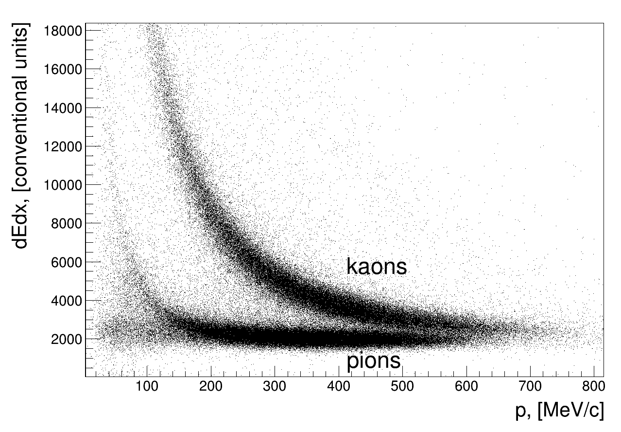
      Figure 2: The $(dE/dx)_{\rm DC}$ distribution for the simulated kaons and pions in $K^{+}K^{-}\pi^{+}\pi^{-}$ final state.

      

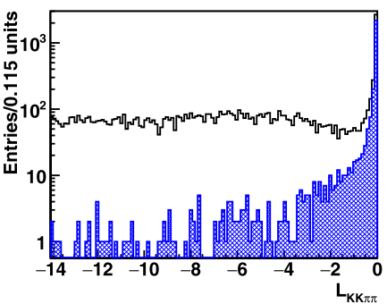
      Figure 3: The $L_{2K2\pi}$ distribution for the 4-tracks events for data (open histogram) and $K^{+}K^{-}\pi^{+}\pi^{-}$ simulation (blue histogram). The cut $L_{2K2\pi}>-3.0$ is applied to avoid misidentification. All c.m. energy points are combined.

      

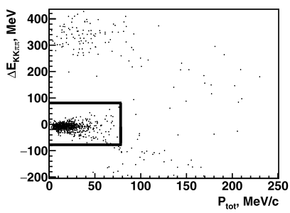
      Figure 4: The energy disbalance vs. total momentum for the 4-tracks events after kaon/pion separation (data, $E_{\rm c.m.}=1.98{\,}\rm GeV$). The events inside the frame are considered to be signal.

      

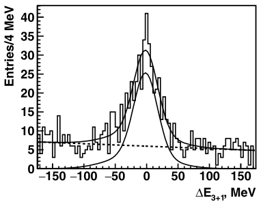
      Figure 5: The signal/background separation by fitting the energy disbalance distribution for 3-tracks events (data, $E_{\rm c.m.}=1.98{\,}\rm GeV$).

      The cross section measurement for $e^{+}e^{-}{\to}K^{+}K^{-}\pi^{+}\pi^{-}$ process requires the amplitude analysis of the final state production. The major intermediate mechanisms were found to be:

      • $f_{0}(500,980)\phi(1020)$;

      • $\rho(770)(KK)_{\rm S-wave}$;

      • $(K_{1}(1270,1400)K)_{\rm S-wave}{\to}(K^{\ast}(892)\pi)_{\rm S-wave}K$;

      • $(K_{1}(1400)K)_{\rm S-wave}{\to}(\rho(770)K)_{\rm S-wave}K$.

      The relative amplitudes of these mechanisms at each c.m. energy point were found using the unbinned fit of the data, see the Monte-Carlo-data comparison after the fit in Figs. 6a– 6d.

      

      

      

      

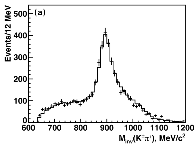
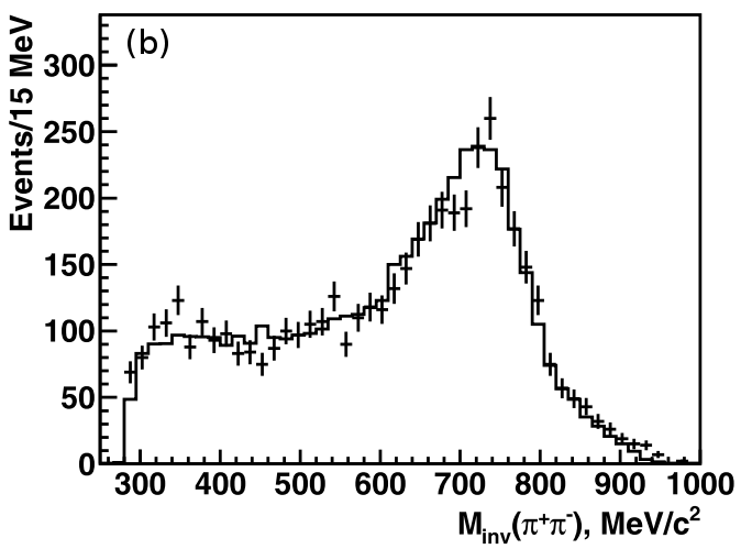
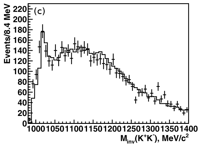
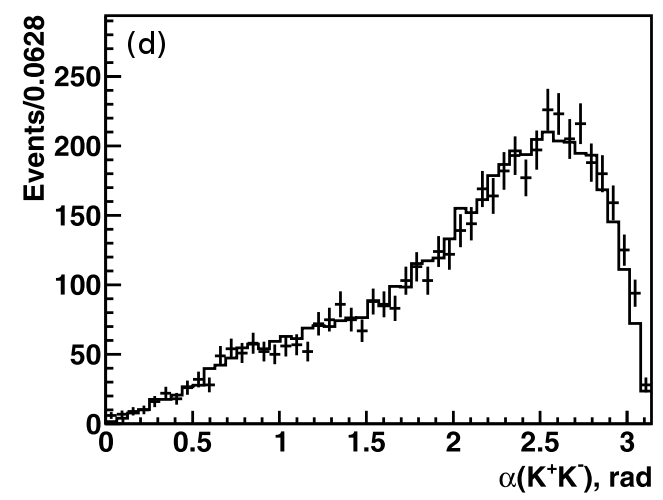
      Figure 6: The distributions of the $K^{\pm}\pi^{\mp}$ (a), $\pi^{+}\pi^{-}$ (b), $K^{+}K^{-}$ (c) invariant masses and the angle between momenta of kaons (d). Data (points) and simulation (open histogram) for $E_{\rm c.m.}=1.95{\,}\rm GeV$.

      The results for the cross section measurement, based on the runs of 2011-2012 (published in [7]), are shown in Fig. 7. The preliminary results of the analyzis of new data of 2017 show a drop of about $10\%$ in the visible cross section at $p\bar{p}$ threshold (see Fig. 8), similar to that in $e^{+}e^{-}{\to}3\pi^{+}3\pi^{-}$ cross section [9]. Such a drop at $p\bar{p}$ threshold is firstly observed in the final state with kaons, and, being confirmed, will require theoretical explanation.

      

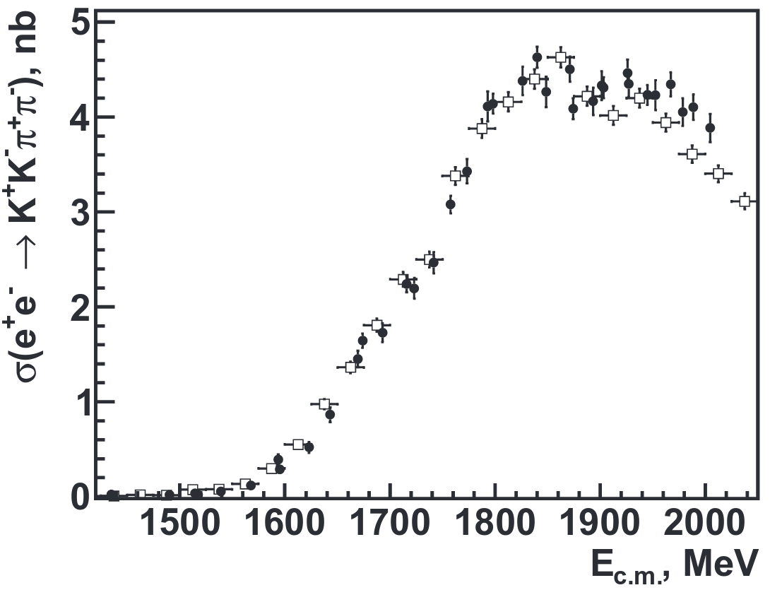
      Figure 7: The $e^{+}e^{-}{\to}K^{+}K^{-}\pi^{+}\pi^{-}$ cross section, measured on the base of the runs of 2011-2012 years (black circles), along with the BaBar results (open bars) [8].

      

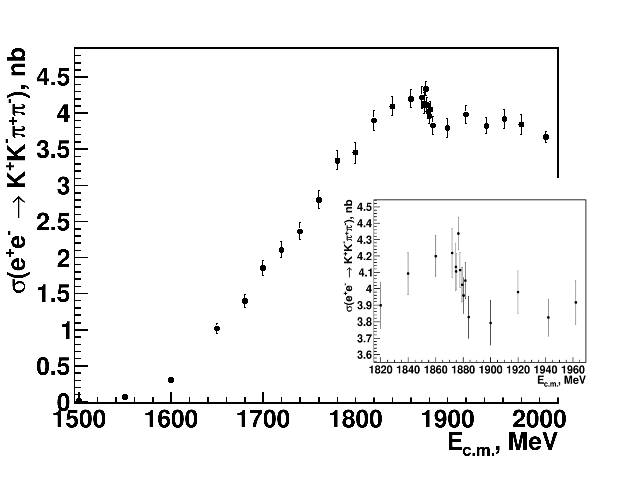
      Figure 8: The visible cross section of $e^{+}e^{-}{\to}K^{+}K^{-}\pi^{+}\pi^{-}$ process with the drop at $p\bar{p}$ threshold (on the base of 2017 year runs).

   3. Study of the $e^{+}e^{-}{\to}K^{+}K^{-}\eta,{\,}K^{+}K^{-}\omega(782)$ processes

      The study of $e^{+}e^{-}{\to}K^{+}K^{-}\eta,{\,}K^{+}K^{-}\omega(782)$ processes has been performed on the base of $19$ pb^-1 of data, collected in 2011-2012. In these two analyzes the $\eta$ and $\omega(782)$ were treated as the recoil particles. The events with 2, 3 and 4 DC-tracks were considered. The kaon/pion separation was performed using the LLF maximization and cuts on $L_{2K}$, $L_{2K\pi}$ and $L_{2K2\pi}$, see Fig. 10. The $K^{+}K^{-}\pi^{+}\pi^{-}$ final state dominates the background in 3 and 4-tracks classes, but we suppress it’s contribution by the cuts on the $2K\pi$ and $2K2\pi$ missing masses, see Fig. 10. Since we observed only $\phi(1020)\eta$ intermediate mechanism of $K^{+}K^{-}\eta$ production, we applied the cut on the $K^{+}K^{-}$ invariant mass to select the $\phi(1020)$ meson region, see Fig. 12. The signal/background separation in both processes is performed by approximation of the $K^{+}K^{-}$ missing mass distribution, see Fig. 12. The preliminary results for the cross sections are shown in Figs. 14–14.

      

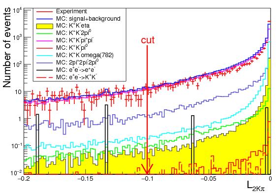
      Figure 9: The distribution of $L_{2K\pi}$ parameter in the experiment and simulation of signal and major background processes. All c.m. energy points are combined.

      

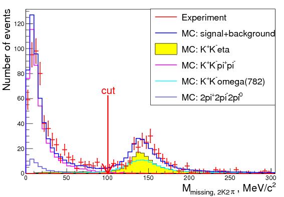
      Figure 10: The distribution of the $2K2\pi$ missing mass in the experiment and simulation of signal and major background processes. All c.m. energy points are combined.

      

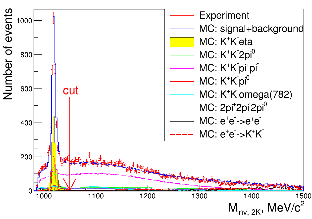
      Figure 11: The distribution of $K^{+}K^{-}$ invariant mass in the experiment and simulation of signal and major background processes. All c.m. energy points are combined.

      

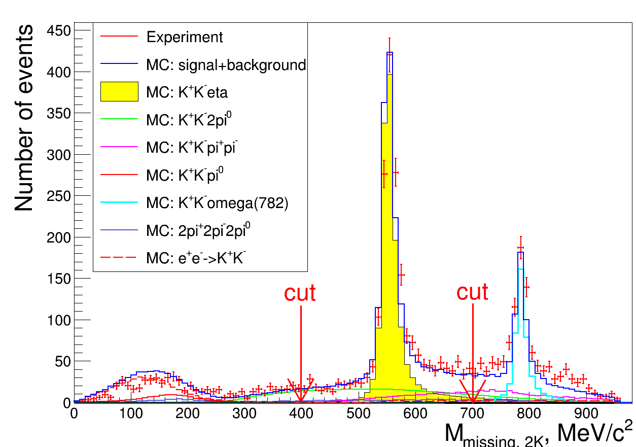
      Figure 12: The distribution of $K^{+}K^{-}$ missing mass in the experiment and simulation of signal and major background processes. All c.m. energy points are combined.

      

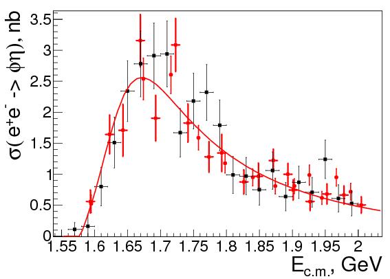
      Figure 13: The results for the $e^{+}e^{-}{\to}K^{+}K^{-}\eta$ cross section (red - CMD-3, preliminary; black - BaBar [10]).

      

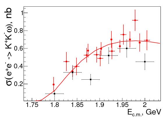
      Figure 14: The results for the $e^{+}e^{-}{\to}K^{+}K^{-}\omega(782)$ cross section (red - CMD-3, preliminary; black - BaBar [11]).

      Since the $\phi(1020)\eta$ production is dominated by $\phi(1680)$ meson decay, the approximation of the $e^{+}e^{-}{\to}\phi(1020)\eta$ cross section allows us to measure the $\phi(1680)$ parameters. We perform the approximation using the following formula:

      $$F(s)={\Biggl{|}}A_{\rm non-\phi^{\prime}}(s)e^{i\Psi}+\sqrt{\frac{(\Gamma^{\phi^{\prime}}_{ee}\mathcal{B}(\phi^{\prime}{\to}\phi\eta))\Gamma_{\phi^{\prime}}m^{3}_{\phi^{\prime}}}{|\vec{p}_{\phi}(m_{\phi^{\prime}})|^{3}}}D_{\phi^{\prime}}(s){\Biggr{|}}^{2}.$$ (2)

      In these formulae $D_{\phi^{\prime}}(s)=1/(s-m^{2}_{\phi^{\prime}}+i\sqrt{s}\Gamma_{\phi^{\prime}}(s))$ and $D_{\phi}(p^{2}_{\phi})=1/(p^{2}_{\phi}-m^{2}_{\phi}+i\sqrt{p^{2}_{\phi}}\Gamma_{\phi}(p^{2}_{\phi}))$ are the inverse denominators of the $\phi$ and $\phi^{\prime}$ propagators, $|\vec{p}_{\phi}(\sqrt{s})|$ is the momentum of the $\phi$ in the $\phi^{\prime}{\to}\phi\eta$ decay in $\phi^{\prime}$ rest frame, $|\vec{p}_{K}(\sqrt{p^{2}_{\phi}})|$ is the momentum of the kaon in the $\phi{\to}K^{+}K^{-}$ decay in $\phi$ rest frame, $\theta_{\rm normal}$ is the polar angle of the normal to the plane, formed by the $\vec{p}_{K^{+}}$ and $\vec{p}_{K^{-}}$ vectors, $d\Phi_{K^{+}K^{-}\eta}$ is the element of three-body phase space, the function $A_{\rm non-\phi^{\prime}}(s)=a/s$ is introduced to describe the possible contribution of the resonances apart from $\phi^{\prime}$ ($a$ is a constant), $\Psi$ is the relative phase between two amplitudes. The results of the fit, shown in the Table 1, are in good agreement with those in BaBar study [10].

      For the $\sigma(e^{+}e^{-}{\to}K^{+}K^{-}\omega(782))$ approximation we used the shape, obtained from the integration of the squared matrix element of $e^{+}e^{-}{\to}\phi^{\prime}{\to}K^{+}K^{-}\omega(782)$,
      $\omega(782){\to}\rho^{\pm,0}\pi^{\mp,0}{\to}\pi^{+}\pi^{-}\pi^{0}$ decay chain over the 5-body phase space.

      Table 1: The $\phi^{\prime}$ parameters obtained from the fit.

      Parameter	Value
      $\chi^{2}/{\rm n.d.f}$	$46.3/33{\approx}1.4$
      $\Gamma^{\phi^{\prime}}_{ee}\mathcal{B}(\phi^{\prime}{\to}\phi\eta),^{\prime}\rm eV$	$163{\pm}37_{\rm stat}{\pm}6_{\rm mod}$
      $m_{\phi^{\prime}},\rm MeV$	$1690{\pm}12_{\rm stat}{\pm}3_{\rm mod}$
      $\Gamma_{\phi^{\prime}},\rm MeV$	$327{\pm}88_{\rm stat}{\pm}14_{\rm mod}$

   4. Study of the $e^{+}e^{-}{\to}K^{+}K^{-}\pi^{0}$ Process

      The study of $e^{+}e^{-}{\to}K^{+}K^{-}\pi^{0}$ process has been performed on the base of $30$ pb^-1 of data, collected in 2011-2012. The events with two oppositely charged DC-tracks and no less than 2 photons with the $E_{\gamma}>40{\,}\rm MeV$ were considered. Then, assimung energy-momentum conservation, the 4C-kinematic fit was performed with the $\chi^{2}_{4C}<35$ cut, see Fig. 16. The major background sources were found to be $K^{+}K^{-}\gamma$, $K^{+}K^{-}2\pi^{0}$, $K_{S,L}K^{\pm}\pi^{\mp}$, $\pi^{+}\pi^{-}\pi^{0}$, $\pi^{+}\pi^{-}2\pi^{0}$. The suppression of these backgrounds was done using the training of BDT classifiers (see Fig. 16) with the following input variables: 1) $(dE/dx)_{\rm DC}$; 2) momenta and angles of charged particles and photons; 3) missing mass of $K^{+}K^{-}$ system. The preliminary results for the $e^{+}e^{-}{\to}K^{+}K^{-}\pi^{0}$ cross section are shown in Fig. 17.

      

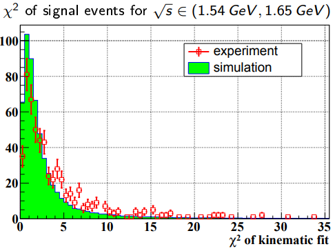
      Figure 15: The distribution of the $\chi^{2}$ of the 4C-kinematic fit of the events (red - experiment, green - simulation of signal process). The energy points in range $1.54{\,}\rm GeV<E_{\rm c.m.}<1.65{\,}\rm GeV$ are combined.

      

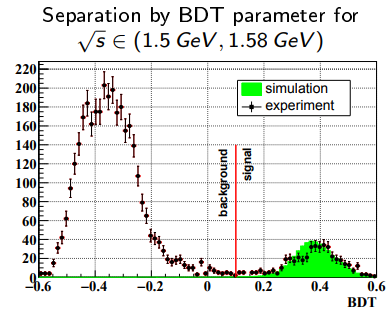
      Figure 16: The distribution of the BDT response of the events (red - experiment, green - simulation of signal process). The energy points in range $1.5{\,}\rm GeV<E_{\rm c.m.}<1.58{\,}\rm GeV$ are combined.

      

      Figure 17: The results for the $e^{+}e^{-}{\to}K^{+}K^{-}\pi^{0}$ cross section (blue and red - CMD-3 2011-2012, preliminary; black - BaBar [10]).

4. Conclusion

   The current status of the study of processes of $e^{+}e^{-}{\to}KK(n)\pi$ with the CMD-3 detector was considered. The CMD-3 has alredy collected about $100$ pb^-1 of data and now is continuing datataking to collect about 1 fb^-1 in the next few years. We are in good disposition to provide the best precision for the $\phi(1680)$ vector meson parameters and to perform the study of $KK(n)\pi$ final states in all charge modes to test the isotopic relations between them. The drop in the $e^{+}e^{-}{\to}K^{+}K^{-}\pi^{+}\pi^{-}$ cross section, seen in the preliminary analysis of the data of 2017 year runs, is firstly observed in the final state with kaons, and, being confirmed, will require theoretical explanation.

5. Acknowledgments

   We thank the VEPP-2000 personnel for the excellent machine operation. The work was supported by the Russian Fund for Basic Research grants RFBR 15–02–05674–a, RFBR 14–02–00580–a, RFBR 16–02–00160–a, RFBR 17–02–00897–a. Part of this work related to the photon reconstruction algorithm in the electromagnetic calorimeter is supported by the Russian Science Foundation (project No. 14–50–00080).

3.11 The GlueX Meson Program

Justin Stevens (for the GlueX Collaboration

Department of Physics

College of William & Mary

Williamsburg, VA 23187, U.S.A.

1. Meson Photoproduction

   The GlueX experiment, shown schematically in Fig. 1, utilizes a tagged photon beam derived from Jefferson Lab’s 12 GeV electron beam. Coherent bremsstrahlung radiation from a thin diamond wafer, yields a linearly polarized photon beam with a maximum intensity near 9 GeV. The primary goal of the experiment is to search for and ultimately study an unconventional class of mesons, known as exotic hybrid mesons which are predicted by Lattice QCD calculations [1].

   

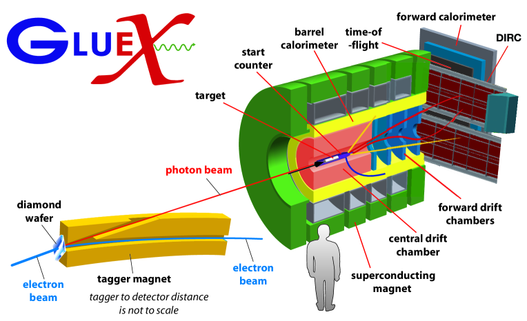
   Figure 1: A schematic of the Hall D beamline and GlueX detector at Jefferson Laboratory. The DIRC detector upgrade will be installed directly upstream of the time-of-flight detector in the forward region.

   

   

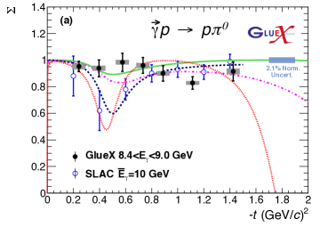
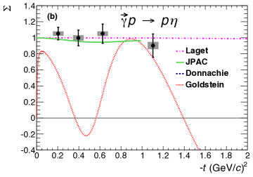
   Figure 2: Beam asymmetry $\Sigma$ for (a) $\pi^{0}$ and (b) $\eta$ photoproduction from Ref. [2].

   To pursue the search for exotic hybrid mesons in photoproduction the production of conventional states, such as pseudoscalar and vector mesons, must first be understood. Previous measurements of pseudoscalar photoproduction at these energies are limited, especially for the linearly polarized beam asymmetry $\Sigma$. This asymmetry provides direct information on the quantum numbers of the $t-$channel Reggeon exchange, with $\Sigma=1$ for purely “natural" exchange (e.g. $J^{P}=1^{-}$) and $\Sigma=-1$ for “unnatural" exchange (e.g. $J^{P}=1^{+}$). First measurements from GlueX [2] indicate that the natural vector meson exchange is dominant in this regime for $\pi^{0}$ and $\eta$ meson production, as seen in Fig. 2. Further studies of the beam asymmetry and polarization observables for other reactions will provide critical insights into the meson photoproduction mechanisms in this energy regime.

2. DIRC Upgrade

   As described above, an initial physics program to search for and study hybrid mesons which decay to non-strange final state particles is well underway. However, an upgrade to the particle identification capabilities of the GlueX experiment is needed to fully exploit its discovery potential, by studying the quark flavor content of the potential hybrid states.

   This particle identification upgrade for GlueX will utilize fused silica radiators from the BaBar DIRC (Detection of Internally Reflected Cherenkov light) detector [3], with new, compact expansion volumes to detect the produced Cherenkov light. The GlueX DIRC will provide $\pi/K$ separation for momenta up to 4 GeV, significantly extending the discovery potential of the GlueX program [4]. The charged kaon identification provided by the DIRC may also yield useful identification of charged kaons for the $K_{L}$ beam facility (KLF) proposed for Hall D [5]. This may be particularly relevant in the production of strange mesons from the high momentum component of the $K_{L}$ beam, where the charged kaons are produced at forward angles.

3. Acknowledgments

   This work is supported by the Department of Energy Early Career Award contract DE–SC0018224.

3.12 Strange Meson Spectroscopy at CLAS and CLAS12

Alessandra Filippi

I.N.F.N. Sezione di Torino

10125 Torino, Italy

1. Introduction

   The identification of states containing open and hidden strangeness is still an open issue in light meson spectroscopy investigations. Apart form a handful of confirmed states, still little is known, for instance, about the radial excitations of the $\phi(1020)$ meson, and even less about strangeonia with quantum numbers other than $1^{--}$. Below 2.1 GeV just about half the open strangeness kaonia states (composed by a strange and a light quark) expected by the Constituent Quark Model (CQM) [1] have been observed so far, while less than ten strangeonia states, mesons of $\bar{s}s$ structure, have been steadily observed out of a total of at least 20 expected states.

   Nonetheless, the knowledge of the properties of such states can provide important inputs for hadron spectroscopy. Strangeonia, in fact, feature an intermediate mass between the heavier systems where the quark model is approximately valid and the lighter meson sector. Unfortunately, their experimental signatures are less clear as compared to charmonium states, as they are broader and lie in a mass range where the overlap probability with other light quark states is very strong, and moreover most of the decay channels modes are shared among all of them.

   To further complicate the problem, in the same mass region some other structures of exotic composition ($\bar{q}qg$ states, known as hybrids, $ggg$ states, the so-called glueballs, or even molecular states of multi-quark composition) are expected by QCD. Recent QCD calculations on the lattice are able to predict most of the conventional meson spectrum in good agreement with experimental findings [2]; these confirmations of course strengthen the confidence in their predictive power for the searches of new states. According to these calculations, the lightest hybrids and glueballs are predicted in the 1.4–3 GeV mass range: namely, at 2 GeV for the lightest $J^{PC}=0^{+-}$ state, and at 1.6 GeV for the $1^{-+}$ one. This is actually the mass region where signatures of still unobserved strangeonia or kaonia are expected to show up, and indeed a number of candidates for exotics has been suggested over the years, still all awaiting for confirmation, fitting the same slots where strangeonia would be expected.

   The use of photons as probes to study strangeness was not used extensively in the past due to the small production rates, and the lack of beams of suitable intensity and momentum resolution. In fact, the production of strange quarks in a non-strange environment involves disconnected quark diagrams whose occurrence is suppressed as a consequence of the OZI rule. However, a good step forward is expected from the results obtained with the photon beam produced by brehmsstrahlung from the continuous electron beam at the CEBAF machine at JLAB.

   Smoking guns for the existence of open and hidden strangeness states would by their observations in the $\phi\eta$ or $\phi\pi$ invariant mass systems [3]; especially in the first case, due to the strange content of the $\eta$ meson, the production of strangeness should be eased [4]. A typical diagram for the photoproduction of the $\phi\eta$ final state is shown in Fig. 1.

   

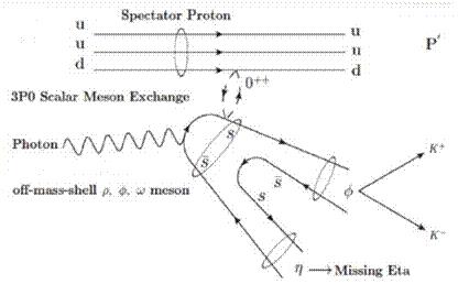
   Figure 1: Quark line diagram for the photoproduction of the $\phi\eta$ final state.

   Very few events in these channels have been observed so far; however, there is a good possibility, as will be shown in Sec. 5, that in the upcoming meson spectroscopy experiment at CLAS12 good samples of such reactions could be collected, opening therefore new opportunities to widen the knowledge of this sector of the meson spectrum.

2. Meson Spectroscopy Studies in Photon Induced Reactions

   Several reactions and beams have been exploited so far for meson spectroscopy searches: among most important, high-energy meson (mainly pion) and proton beams, based on the peripheral and central production mechanisms, antinucleon annihilation at rest and in flight, which convey the formation of a gluon-rich environment suitable for glueball production, and $e^{+}e^{-}$ annihilation. The latter reaction has been studied extensively since the LEP era, and is an environment where also $\gamma\gamma$ collisions can be measured, which provide quite useful information as they are a natural anti-glueball filter. The $e^{+}e^{-}$ annihilation differs from hadronic reactions for the fact that only $1^{--}$ systems can be formed, so these reactions provide naturally a powerful quantum number selection.

   On the other hand, the use of electromagnetic probes, and in particular of photons, in fixed target reactions was not used very extensively for meson spectroscopy purposes, as meantioned earlier. Nevertheless, electromagnetic reactions could deliver important complementary information. In fact, first of all, electromagnetic processes can be exactly reproduced to a high level of precision through QED diagrams thanks to the smallness of the electromagnetic coupling, which is prevented in the case of strong interactions. Moreover, photons can excite with larger probability the production of spin-1 mesons as compared to pion or kaon induced reactions, since in the latter case a spin-flip is required. Therefore, the production of vector hybrid mesons could occur in photoproduction reactions with a rate comparable to those of conventional vector mesons [3, 4]. This feature applies not only to hybrids, but also to spin-1 $\bar{s}s$ excitations.

3. Selected Results from CLAS

   The CLAS apparatus, which had operated up to 2010, is described in detail elsewhere [5]. In the following some selected results from recent meson spectroscopy papers involving strangeness production will be summarized, in connection with some still open issues.

   1. The Scalar Glueball Search Case

      In spite of the efforts by the experiments in the early Nineties, in particular those studying antinucleon annihilations, like Crystal Barrel and OBELIX, the full composition of the scalar meson sector is not completely clear yet. Observations have been made of several mesons whose existence was not foreseen by the CQM; one of them, the $f_{0}(1500)$, seemed to have the right features as lightest scalar glueball candidate [6]. Among these, the most important is the fact that it was observed to decay in several channels, a clear hint to its flavor-blindness. However, more data are still desirable to confirm these properties as several other structures tentatively identified as scalars as well. All the existing observations make the interpretation of the scalar sector difficult, since it is populated more than expected by broad and overlapping states. In this mass region one should also recall the existence of the $\sigma$ state (also known as $f_{0}(600)$), corresponding to a very broad $\pi\pi$ non-resonant iso-scalar $S$-wave interaction, whose nature and properties are still unclear. Also scarcely known are the features of the $\kappa$, the analogous of $\sigma$ observed in the $K\overline{K}$ channel.

      A search was carried on in CLAS exploiting the $\gamma p\rightarrow pK^{0}_{S}K^{0}_{S}$ reaction [7], with real photons of energy in the ranges $(2.7-3)$ and $(3.1-5.1)$ GeV. The $K^{0}_{S}$ were fully reconstructed through their decay in two pions, while the proton was identified from the event missing mass. A strong correlation between the two $K^{0}_{S}$ was found, which allowed to collect a clean sample of good statistics, enough to perform selections in momentum transfer $t(=Q^{2})$. The selection in $t$ is useful to understand the production mechanism of the intermediate states: small values of momentum transfers are correlated to a dominant production from the $t$-channel, while $s$-channel production is characterized by a wider range of transferred momenta. Fig. 2 shows the distributions of the $(K^{0}_{S}K^{0}_{S})$ invariant mass system, after proper background subtraction, in two momentum transfer ranges: for $|t|<1$ GeV² on the left side, and for $|t|>1$ GeV² on the right. A clean peak at about 1500 MeV appears in the first case, while at larger momentum transfer no evidence for it can be observed. This means that the structure at 1500 MeV, a possible indication for the $f_{0}(1500)$ observed in its $K^{0}_{S}K^{0}_{S}$ decay mode, is predominantly produced via $t$-channel. This observation could support its possible interpretation as glueball.

      

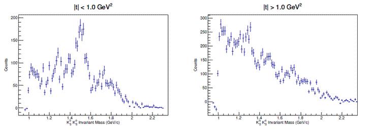
      Figure 2: Invariant mass of the $(K^{0}_{S}K^{0}_{S})$ system for events selected in the $\gamma p\rightarrow pK^{0}_{S}K^{0}_{S}$ reaction, in two momentum transfer ranges: left, for $|t|<1$ GeV², right for $|t|>1$ GeV².

      In order to fully characterize the features of this state a complete spin-parity analysis of the sample is required. Unfortunately, the task is not straightforward due to the limited apparatus acceptance at small forward and backwards angles. Nonetheless, an angular analysis was attempted to test which of the spin-parity hypotheses for the events in the peak region would provide a better fit to the Gottried-Jackson angular distributions.

      We recall that a $(K^{0}_{S}K^{0}_{S})$ bound system may just have $J^{PC}=(even)^{++}$ quantum numbers, so the spin 0 and 2 hypotheses need to be tested. An example of angular distribution is reported in Fig. 3, in a $(K^{0}_{S}K^{0}_{S})$ mass window centered at 1525 MeV. The curves superimposed to the experimental data show the contributions of $S$ and $D$ waves (blue and red, respectively) to the total fit (green). The $D$-wave contribution plays a marginal rôle, larger for masses higher than 1550 MeV, from which one can deduce that the scalar hypothesis for the observed resonance is mostly supported; therefore, it can be more easily identified as the $f_{0}(1500)$.

      

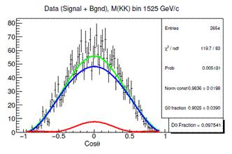
      Figure 3: Gottfried-Jackson angular distribution for $K^{0}_{S}K^{0}_{S}$ events selected in the 1525 MeV invariant mass slice, with superimposed the expected trend, on the basis of Monte Carlo simulations, for production from $S$ wave (blue), $D$ wave (red), and the global fit with the two components (green).

   2. The Axial/Pseudoscalar Sector at 1.4 GeV Case

      Kaonia radial excitations were widely studied in the past together with $\eta$ excitations in the same mass range, to search for possible exotic states. Many observation of $\eta$’s and $f_{1}$ mesons have been reported since the Sixties, when the issue of the overlap of many axial and pseudoscalar states and the difficulty of their identification posed the so-called $E/\iota$ puzzle [8]. While annihilation experiments, and in particular OBELIX, could provide a solution to this puzzle addressing the production of several pseudoscalar and axial states, high statistics photoproduction reactions are expected to deliver new complementary information which will be able to improve the knowledge in this sector.

      A systematic study was performed by CLAS to study the photoproduction of states, decaying into $\eta\pi^{+}\pi^{-}$ and $K^{0}K^{\pm}\pi^{\mp}$ and recoiling against a proton, in the $\gamma p$ reaction with photons in the energy range $(3-3.8)$ GeV [9]. Fig. 4 shows the missing mass plot of the system recoiling against a proton for $\gamma p\rightarrow p\eta\pi^{+}\pi^{-}$ selected events, where a clean signal due to the $\eta^{\prime}(958)$ appears, together with a structure at about 1280 MeV, that can tentatively be identified as the $f_{1}(1285)$.

      

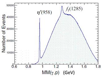
      Figure 4: Missing mass recoling against a proton for events selected in the $\gamma p\rightarrow p\eta\pi^{+}\pi^{-}$ reaction.

      Concerning the reaction witk kaons, the $K^{\pm}$ were identified by CLAS through time of flight techniques, while the $K^{0}$ via the missing mass information. The missing mass plots for the system recoiling against the proton for events selected in the two channels $\gamma p\rightarrow p\overline{K^{0}}K^{+}\pi^{-}$ and $\gamma p\rightarrow p{K^{0}}K^{-}\pi^{+}$ are shown, respectively, in Fig. 5(a) and (b).

      

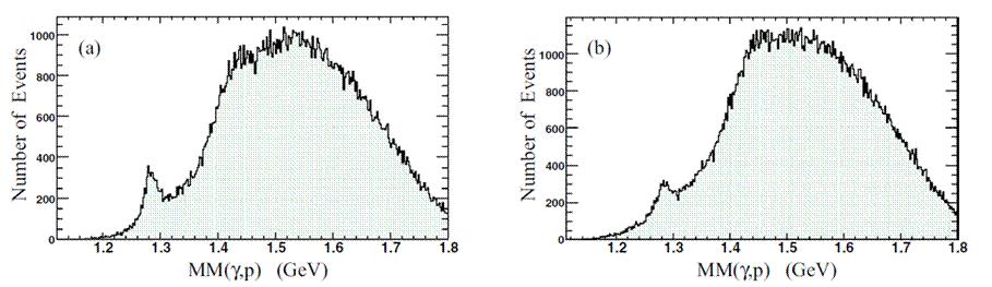
      Figure 5: Missing mass recoling against a proton for events selected in the a) $\gamma p\rightarrow p\overline{K^{0}}K^{+}\pi^{-}$ and b) $\gamma p\rightarrow p{K^{0}}K^{-}\pi^{+}$ reactions.

      In both of them a clear peak appears at about 1.3 GeV, but no further evidence for higher mass states that could be addressed to additional pseudoscalar states, like the $\eta(1405)$ and $\eta(1470)$, or to axial states, as the $f_{1}(1420)$ of $f_{1}(1510)$, is present.

      From the richest $\eta\pi^{+}\pi^{-}$ sample, one can get information for the identification of the observed state. There are a few hints that support the identification as axial $f_{1}(1285)$ against the pseudoscalar $\eta(1295)$. The first one is given by the values obtained for the mass and width of the signal, $M=(1281.0\pm 0.8)$ MeV and $\Gamma=(18.4\pm 1.4)$ MeV, which are closer to those already observed for $f_{1}(1285)$ [10]. The ratio itself of the decay rates in $\eta\pi^{+}\pi^{-}$ versus $K\overline{K}\pi$, that amounts to about five, is consistent with the value quoted by PDG for the $f_{1}(1285)$ decays, while no such ratio was ever measured for $\eta(1295)$ [10].

      The second hint is given by the trend of the differential cross section, for events selected in the band of $\eta^{\prime}(958)$ and around 1280 MeV: as shown in Fig. 6, the two are remarkably different as a function of the center-of-mass angle, indicating a different production mechanism and possibly a different spin configuration of the produced state.

      

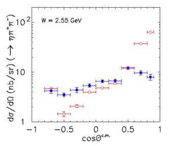
      Figure 6: Differential cross section of the $\gamma p\rightarrow\eta\pi^{+}\pi^{-}p$ reaction for events selected in the $\eta^{\prime}(958)$ mass band (red open points) and the $f_{1}(1285)$ one (blue points). The energy in the center of mass is fixed at 2.55 GeV.

      The comparison of the cross sections for events in the 1280 MeV band with the expectations from $t$-channel based models [11, 12, 13], shown in Fig. 7, indicates clearly a poor match with this production hypothesis: a substantial contribution from $s$-wave could be needed, or a mechanism different from meson exchange involving $N^{\ast}$ excitations or $KK^{\ast}$ molecular interactions. In both cases the identification of the structure as $f_{1}(1285)$ would get larger support.

      

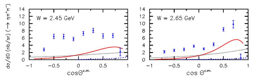
      Figure 7: Differential cross sections of the $\gamma p\rightarrow\eta\pi^{+}\pi^{-}p$ reaction for events selected in the $f_{1}(1285)$ mass band in two center-of-mass energy bins (left: 2.45 GeV, right: 2.85 GeV), compared with a few $t$-channel exchange based models (none of which matches the experimental points): solid red line from Ref. [11], blue dashed line from Ref. [12], black dotted line from Ref. [13].

4. Prospects for CLAS12

   The CLAS12 spectrometer, an upgraded version of CLAS, is a multipurpose facility dedicated to hadron physics studies, from nuclear properties and structure to meson spectroscopy investigations. A full description of CLAS12 is given elsewhere [14]. A second experiment installed on the CEBAF machine, GlueX, is operating in parallel with a program fully committed to meson spectroscopy [15].

   Due to the increased beam energy, as compared to the previous installation, the CLAS12 spectrometer has a more compact structure, which limits its geometric acceptance, although allowing an acceptable hermeticity. However, its detectors feature better momentum resolution and particle identification capabilities as compared to GlueX, therefore the two experimental setups offer complementary qualities.

   While GlueX will use a real photon bremsstrahlung beam, this is not be possible for CLAS12 as the bending dipole magnet available in Hall B will not be powerful enough to steer the 11 GeV electron beam into the tagger beam dump. A new technique was therefore conceived to produce a photon beam for the study of photoproduction reactions, based on electron scattering at very low transferred momentum ($Q^{2}<10^{-1}$ GeV²). In this situation the electrons are scattered at very small polar angles, and the reaction on protons is induced by quasi-real photons. A dedicated part of the CLAS12 apparatus, the Forward Tagger, was devised to detect these forward scattered electrons. For momentum transfers in the interval $0.01<Q^{2}<0.3$ GeV², the electrons scattered between $2.5^{\circ}$ and $4.5^{\circ}$ in polar angle in the lab have an energy in the 0.5–4.5 GeV range, being produced by the interaction of 6.5–10.5 GeV quasi-real photons on protons. Measuring the electron momentum, each virtual photon can be tagged. The use of the CLAS12 spectrometer to measure in coincidence the particles produced in the photoproduction reaction will allow to perform a complete event recontruction, necessary for meson spectroscopy studies. With this tagging technique one can measure also the virtual photon polarization, that is linear and can be deduced, event by event, from the energy and the angle of the scattered electron. The systematic uncertainty affecting the polarization depends only on the electron momentum resolution. High electron currents may be used, therefore a good luminosity can be obtained even with thin targets, that are not operable with real photon bremsstrahlung beams. For instance, using a 5 cm long LH₂ target, the resulting hadronic rate will be equivalent to that achievable by a real photon flux of about $5\times 10^{8}\gamma$/s.

   The Forward Tagger equipment, described in detail in Ref. [16], is located about 190 cm away from the target and fits within a 5^∘ cone around the beam axis. It is made up of:

   • an electromagnetic calorimeter (FT-Cal): composed by 332 PbWO₄ crystals, 20 cm long and with square $15\times 15$ mm² cross-section. It is used to identify the scattered electron and measure its energy, from which the photon energy and its polarization can be deduced (the polarization being given by $\epsilon^{-1}\sim 1+\nu^{2}/(EE^{\prime})$, where $\nu=E-E^{\prime}$ is the photon energy, and $E$ and $E^{\prime}$ the energies of the incident and of the scattered electron, respectively). It is also used to provide a fast trigger signal. Its expected design resolution is $\sigma_{E}/E\sim(2\%/\sqrt{E(\mathrm{GeV})}\oplus 1\%)$;

   • a scintillator hodoscope made of plastic scintillator tiles: located in front of the calorimeter, is used to veto photons; its spatial and timing resolution is required to be comparable with FT-Cal’s;

   • a tracker: located in front of the hodoscope and composed by Micromegas detectors, is used to measure the angle of the scattered electron and the photon polarization plane.

   A sketch of the Forward Tagger region is shown in Fig. 8.

   

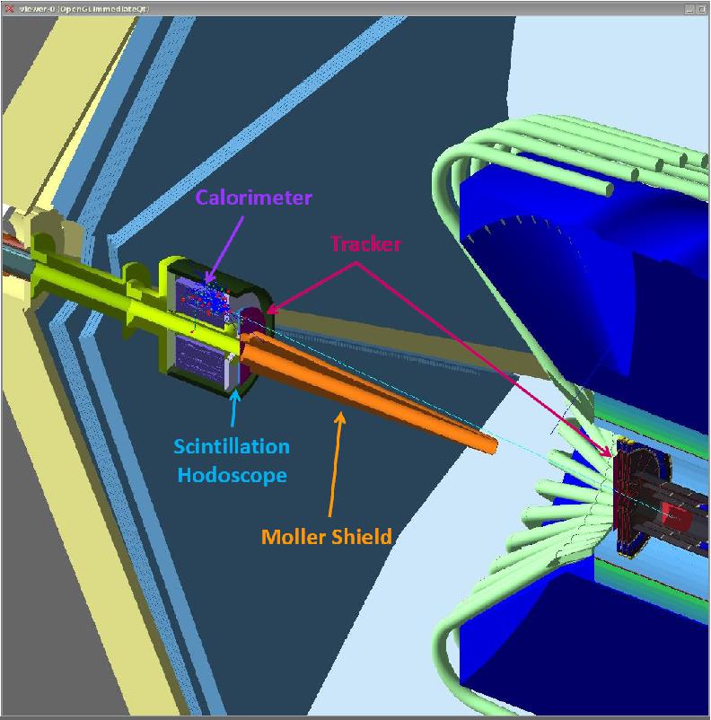
   Figure 8: Schematic view of the Forward Tagger equipment, to be hosted in CLAS12.

5. Strange Meson Spectroscopy with CLAS12

   The Meson-EX experiment at CLAS12 (Exp-11-005 [17]) was proposed to study of the meson spectrum in the 1–3 GeV mass range through quasi-real photon induced reactions, for the identification of gluonic excitations of mesons and other exotic quark configurations beyond CQM. The use of the Forward Tagger will allow to identify the photoproduction reaction on protons through the tagging of the forward scattered electron, while the full CLAS12 apparatus will perform a complete reconstruction and identification of the charged and neutral particles produced in the interaction. Some golden channels have been selected as particularly suitable for the search of exotic or still unknown particles, whose production, as mentioned before, will be favored in photoproduction especially in the case of spin 1 particles. In particular, for the search of hybrids with open strangeness and strangeonia, the following channels are expected to provide interesting new indications: $\gamma p\rightarrow\phi\pi^{0}p$, $\gamma p\rightarrow\phi\eta p$ and $\gamma p\rightarrow K\overline{K}\pi p$. For the first two, extensive simulations were carried over to test the feasibility of such measurements and the expected collectable statistics, in a 80-days long data taking at the full CEBAF luminosity ($\sim 10^{35}\;\mathrm{s}^{-1}\mathrm{cm}^{-2}$) with a total expected trigger rate for photoproduction reactions less than 10 kHz. Assuming an apparatus acceptance for four track events of the order of 15%, it will be possible to collect as many as 3000 events per 10 MeV mass bin, for reactions with a cross section as small as 10 nb, expected for instance for strangeonia production. This statistics is considered to be enough to perform detailed partial-wave analysis studies.

   More in detail, concerning the $\phi\eta$ channel and the possible production of the $\phi(1850)$ excitation, simulations showed that an overall acceptance of about 10% can be expected, due to the coverage at small angles provided by the Forward Tagger electromagnetic calorimeter in which the photons from the $\eta$ decay can be detected. The full event would be reconstructed identifying, in addition, at least one of the kaons from the $\phi$ decay and the recoiling proton, the $K^{-}$ being identifiable through the reaction missing mass. A cross section on the order of 10 nb is tentatively expected, given an existing estimation by the CERN Omega Collaboration [18] of about 6 nb at higher energies, for the production of $\phi(1850)$ and its decay in the $K^{+}K^{-}$ mode, whose branching ratio is expected to be about twice as large as compared to $\phi\eta$.

   On the other hand, concerning the $\phi\pi^{0}$ intermediate state which could be a possible source of exotic systems, again a resonable detection efficiency could be achieved requiring a full identification of the positive kaon from the $\phi$ and the reconstruction of the $\pi^{0}$ through two photons in the Forward Tagged calorimeter. The negative kaon acceptance, largely reduced as it bends inwards at small angles, therefore in a region of scarce detector coverage, can be recovered identifying the particle via the missing mass information; this of course demands again a good resolution on the photon energy. In these conditions, an acceptance similar to those of more “conventional” intermediate states (composed for instance by pions only) can be expected, with basically no impact by the chosen intensity of the magnetic field.

6. Conclusion

   Nowadays many communities are involved all over the world in hadron spectroscopy studies, both from experimental and from the theoretical point of view. Experimental facilities are presently delivering, and will deliver in the near future, large amounts of good quality data that will allow to extract for the first time, from different reactions and experimental environments, new information on many still unsolved issues.

   Photoproduction experiments at JLab will play a big role in the coming future. At JLab, GlueX and CLAS12 will provide data samples of unprecedented quality and richness. Their contribution is expected to grow to sizeable relevance and have a big impact in the present and future meson spectroscopy experimental scenario, complementing the information that will be provided by $e^{+}e^{-}$ collisions (by BESIII and BelleII), by pion induced interactions (by COMPASS), by proton-proton interactions (at fixed target by LHCb, and in high-energy $pp$ collisions by ATLAS and CMS) and by antiproton-proton annihilations (by PANDA at FAIR).

3.13 Dispersive Determination of the $\pi-K$ Scattering Lengths

Jacobo Ruiz de Elvira, Gilberto Colangelo, and Stefano Maurizio

Albert Einstein Center for Fundamental Physics

Institute for Theoretical Physics, University of Bern

3012 Bern, Switzerland

1. Introduction

   Pion-kaon scattering is one of the simplest processes to test our understanding of the chiral symmetry-breaking pattern in the presence of the strange quark. In particular, its low-energy parameters, most notably the scattering lengths, encode relevant information about the spontaneous and explicit chiral symmetry breaking in this sector. Being low-energy observables, their properties can be efficiently studied using the effective field theory of Quantum Chromodynamics (QCD) at low energies, Chiral Perturbation Theory (ChPT) [1, 2, 3], constructed as a systematic expansion around the chiral limit of QCD in terms of momenta and quark masses.

   Pion-kaon scattering can be expressed in terms of two independent invariant amplitudes with well defined isospin $I=1/2$ and $I=3/2$ in the $\pi K\to\pi K$ channel, namely $T^{1/2}$ and $T^{3/2}$. Nevertheless, for convenience, it is useful to combine them in terms of isospin-even and -odd amplitudes $I=\pm$, which are defined as

   $$T_{ab}=\delta_{ab}T^{+}+\frac{1}{2}\left[\tau_{a},\tau_{b}\right]T^{-},$$ (1)

   where $a$ and $b$ denote pion isospin indices and $\tau_{a}$ stand for the Pauli matrices. Both basis are related by simple isospin transformations:

   $$T^{1/2}=T^{+}+2T^{-},\qquad T^{3/2}=T^{+}-T^{-}.$$ (2)

   At leading order (LO) in the chiral expansion, i.e., in the expansion in pion and kaon masses and momenta, the scattering amplitude is given by the Feynman diagram shown in Fig. 1a,

   

   

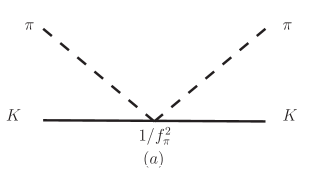
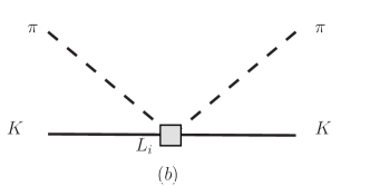
   Figure 1: (a) Leading-order diagrams for $\pi K$ scattering in chiral perturbation theory. Kaon are denoted by full, pions by dashed lines. (b) Next-to-leading-order diagrams depending on low-energy constants $L_{1-8}$.

   resulting in the well-known low-energy theorems for the $S$-wave scattering lengths, the amplitudes evaluated at threshold [3, 4]:

   $$a^{-}_{0}=\frac{m_{\pi}m_{K}}{8\pi(m_{\pi}+m_{K})f_{\pi}^{2}}+\mathcal{O}\big{(}{m_{i}^{4}}\big{)},\qquad a^{+}_{0}=\mathcal{O}\big{(}{m_{i}^{4}}\big{)},$$ (3)

   where $m_{i}$ denotes the pion ($m_{\pi}$) or kaon ($m_{K}$) mass. The isospin-odd scattering length is hence predicted solely in terms of the pion and kaon masses as well as the pion decay constant $f_{\pi}$, while the isospin-even one is suppressed at low energies. The LO ChPT value for the pion-kaon scattering lengths is denoted by a star in Fig. 2, where the pion-kaon scattering length plane is plotted in the $I=1/2$ and $I=3/2$ basis.

   

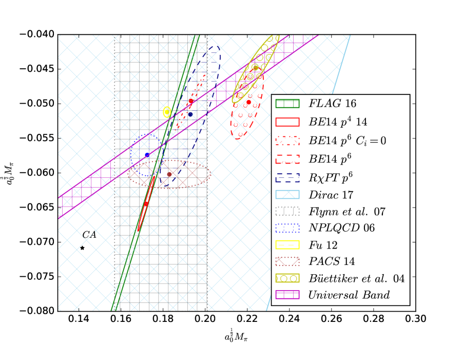
   Figure 2: Different determinations of the pion-kaon scattering lengths in the $I=1/2$, $I=3/2$ basis. The LO ChPT value, just a result of current algebra, is denoted by a star. The NLO prediction of the isospin-odd scattering length is given by the dark-green band labelled as FLAG16. The inclusion of the isospin-even scattering length, using the LECs provided in Ref. [8], leads to the solid-red ellipse BE14 $p^{4}$. The red dot-dashed ellipse, BE14 $p^{6}$ $C_{i}=0$, corresponds to the NNLO chiral prediction when the $\mathcal{O}\big{(}p^{6}\big{)}$ LECs are set to zero. The full NNLO result is represented by the dashed-red ellipse, albeit, as explained in the text, this result is biased to reproduce the RS dispersive values given in Ref. [10], solid-green ellipse. The NNLO results with $\mathcal{O}\big{(}p^{6}\big{)}$ LECs estimated by resonance saturation is denoted by the dashed-blue ellipse, $R\chi PT$ $p^{6}$. The universal band obtained from the RS analysis performed in this work is given by the violet band. The remaining experimental and lattice results are explained in the main text.

   The pion-kaon scattering amplitude at next-to-leading order (NLO) was derived and studied first in [5, 6]. It involves one-loop diagrams, which might generate large contributions. Nevertheless, they are suppressed at threshold and hence their role for the pion-kaon scattering lengths is relatively small. In addition, the $\pi K$ scattering amplitude depends at NLO on a list of low-energy constants (LECs), conventionally denoted by $L_{1-8}$, which, encoding information about heavier degrees of freedom, can not be constrained from chiral symmetry solely, Fig. 1b. Once determined in one process, these LECs can subsequently be used to predict others. The NLO pion-kaon scattering lengths were analyzed in detail in [5]. The contribution from the LECs reads [5]:

   $$a^{-}_{0}\big{|}_{\mathrm{LECs}}= \frac{m_{K}m_{\pi}^{3}}{\pi(m_{\pi}+m_{K})f_{\pi}^{4}}L_{5}+\mathcal{O}\big{(}m_{i}^{6}\big{)},$$ (4)

   $$a^{+}_{0}\big{|}_{\mathrm{LECs}}= \frac{m_{K}^{2}m_{\pi}^{2}}{\pi(m_{\pi}+m_{K})f_{\pi}^{4}}\left(4(L_{1}+L_{2}-L_{4})+2L_{3}-L_{5}+2(2L_{6}+2L_{8})\right)+\mathcal{O}\big{(}m_{i}^{6}\big{)}.$$

   On the one hand, whereas the NLO LECs contribution to the isospin-odd scattering length is suppressed by a $m_{\pi}^{3}$ factor, the isospin-even scattering length is proportional to $m_{K}^{2}$. Thus, one should expect a small higher-order correction in the chiral expansion for $a^{-}_{0}$ but a much larger shift for $a^{+}_{0}$. On the other hand, while the isovector scattering length only depends on one LEC, $L_{5}$, which is indeed well constrained from the pion and kaon mass and decay constant values, the isoscalar scattering length involve seven LECs and hence sizable uncertainties for this quantity associated with LECs errors are expected. The constraint imposed by the isovector scattering length at NLO in ChPT is depicted by a dark-green band in Fig. 2, where the central value and error for $L_{5}$ is taken from the FLAG group estimate [7]. Note that the small width of this band is completely determined by the $L_{5}$ uncertainty. Furthermore, using the LECs collected in Table 1 in Ref. [8] (first column), one can also include the NLO prediction for the isoscalar scattering length, which leads to the solid-red ellipse in Fig. 2. As we have already anticipated, this ellipse is stretched out in the isoscalar direction but shrunk in the isovector one.

   One might wonder how stable are the NLO predictions against higher-order corrections. A pion-kaon low-energy theorem [5] imposes higher $\mathcal{O}\big{(}{m_{i}^{2\,n}}\big{)}$ contributions to the isospin-odd scattering length arising from contact terms to be at most:

   $$a^{-}_{0}\big{|}_{N^{n}LO}\propto a^{-}_{0}\big{|}_{LO}\,\left(\frac{m_{\pi}}{4\pi f_{\pi}}\right)^{2}\,\left(\frac{m_{K}}{4\pi f_{\pi}}\right)^{2\,n}\quad\textrm{with}\quad n\geq 2.$$ (5)

   Whereas the factor $(m_{K}/4\pi f_{\pi})\sim 0.2$ is relatively large, the prefactor $m_{\pi}^{2}/(4\pi f_{\pi})^{2}\sim 0.015$ suppresses higher order corrections by roughly two orders of magnitude, i.e., the isospin-odd scattering length is protected from higher-order correction and hence one should expect small deviations from the NLO ChPT prediction for $a_{0}^{-}$.

   The pion-kaon scattering amplitude at next-to-next-to-leading order (NNLO) in the chiral expansion was derived in [9]. It involves a set of 32 new $\mathcal{O}\big{(}p^{6}\big{)}$ LECs, the so called $C_{1-32}$, which unfortunately are still not well constrained from experiment. As a first step, one could estimate the size of the NNLO chiral corrections by setting all the $C_{i}$ to zero. Using for the $\mathcal{O}\big{(}p^{4}\big{)}$ $L_{i}$ the corresponding fit in [8], the outcome is the red dot-dashed ellipse plotted in Fig. 2. This result is consistent with our previous statement, i.e., whereas the shift between the NLO and NNLO ellipsis is small in the isovector direction, it is much larger in the isoscalar one.

   The $C_{i}$ entering in pion-kaon scattering were also estimated in [8] by performing a global fit to different $\pi\pi$ and $\pi K$ observables. Nevertheless, among them, the dispersive determination of the $\pi K$ scattering lengths in [10] was used as constraint. Consequently, the full $\mathcal{O}\big{(}p^{6}\big{)}$ results in [8] are not a genuine ChPT prediction but they are biased to satisfy the results given in [10]. The scattering length results in [8] and [10] are denoted in Fig. 2 by the dashed-red and dashed-green circle-filled ellipse, respectively. As we will discuss in detail below, the large difference one finds between the NLO and NNLO chiral estimates in the isovector direction is just a consequence of the large discrepancy between the dispersive result in [10] and chiral expectations. Alternatively, one can estimate the value of the $C_{i}$ by using resonance saturation. The contribution from vector and scalar resonances to the saturation of the $\mathcal{O}\big{(}p^{6}\big{)}$ LECs was also studied in [9]. Using the vector and scalar resonance parameter values extracted in [11] from a global $\pi\pi$ and $\pi K$ fit, one obtains the dashed-blue ellipse in Fig. 2, which is now consistent with the NLO prediction for the isovector scattering length.

   The only direct experimental information about the pion-kaon scattering lengths comes from the DIRAC experiment at CERN [12], where the lifetime of hydrogen-like $\pi K$ atoms was measured. They are a electromagnetically bound state of charged pions and kaons, $\pi^{+}K^{-}$ and $\pi^{-}K^{+}$, which decay predominantly by strong interactions to the neutral pairs $\pi^{0}\bar{K}^{0}$ and $\pi^{0}K^{0}$. The $\pi K$ atom lifetime and the scattering length are related through the so-called modified Deser formula [13, 14, 15], namely

   $$\Gamma_{1S}=8\alpha^{3}\mu^{2}p\,a_{0}^{-\,2}\left(1+\delta_{K}\right),$$ (6)

   where $\alpha$ is the fine structure constants, $\mu$ is the reduced mass of the $\pi^{\pm}K^{\mp}$ system, $p$ is the outgoing momentum in the centre-of-mass frame and $\delta_{K}$ accounts for isospin breaking corrections [14, 15, 16]. The experimental determination of $\Gamma_{1S}$ obtained at CERN yields [12]

   $$a_{0}^{-}=\left(0.072^{+0.031}_{-0.020}\right)\,m_{\pi}^{-1},$$ (7)

   which is denoted in Fig. 2 by a light-blue squared-filled band. Unfortunately, the experimental errors are still too large to provide useful information about the pion-kaon scattering lengths. Nevertheless, there is still room for improvement, the statistical precision is expected to improve by a factor 20 if the DIRAC Collaboration manages to run its experiment using the LHC 450 GeV proton beam. The proposed kaon beam experiment at JLab could certainly help to improve the current experimental information about the pion-kaon scattering lengths.

   On the lattice side, there is a plethora of results and we will only consider unquenched analyses. From a lattice analysis of the $\pi K$ scalar form factor in semileptonic $K_{l3}$ decays, the value $a_{0}^{1/2}=0.179\left(17\right)\left(14\right)\,m_{\pi}^{-1}$ was reported in [17] for the pion-kaon scattering length in the $I=1/2$ channel. This value corresponds to the gray squared-filled band in Fig. 2. The first fully dynamical calculation with $N_{f}=2+1$ flavors was performed by the NPLQCD collaboration, leading to [18]

   $$a_{0}^{1/2}=\left(0.173^{+0.003}_{-0.016}\right)\,m_{\pi}^{-1},\quad a_{0}^{3/2}=\left(-0.057^{+0.003}_{-0.006}\right)\,m_{\pi}^{-1},$$ (8)

   which is denoted in Fig. 2 by a dotted-blue ellipse. Further dynamical results for $N_{f}=2+1$ flavors were reported in [19] using a staggered-fermion formulation, $a_{0}^{1/2}=0.182\left(4\right)\,m_{\pi}^{-1},\quad$
   $a_{0}^{3/2}=-0.051\left(2\right)\,m_{\pi}^{-1}$, and by the PACS collaboration considering an improved Wilson action [20], $a_{0}^{1/2}=0.183\left(18\right)\left(35\right)\,m_{\pi}^{-1},\quad a_{0}^{3/2}=-0.060\left(3\right)\left(3\right)\,m_{\pi}^{-1}$. These results are depicted in Fig. 2 by a solid-yellow and a dotted-brown ellipse, respectively.

   As we have seen, all the previous results are consistent with chiral predictions, i.e., all of them are consistent within one standard deviation for the isospin-odd direction, whereas much larger differences are found in the isospin-even component. Nevertheless, the most precise up-to-date result was reported in [10] by solving a complete system of Roy-Steiner equations, corresponding to

   $$a_{0}^{1/2}=0.224(22)m_{\pi}^{-1},\quad a_{0}^{3/2}=-0.045(8)m_{\pi}^{-1}.$$ (9)

   This result is denoted in Fig. 2 by a light-green circle-filled ellipse and it lies more than 3.5 standard deviations away from the NLO ChPT result. This disagreement is particularly puzzling in the isospin-odd direction, where the ChPT prediction is protected by the low-energy theorem given in (5) and one should expect NLO ChPT to provide a reasonably precise value for the pion-kaon scattering lengths. In fact, previous dispersive analyses for $\pi\pi$ scattering provided results for the scattering lengths only within a universal band [22, 23]. High accuracy values were reached only after constraining dispersive results with chiral symmetry. Thus, one might wonder why should things be different in pion-kaon scattering. In the remaining part of this talk we will try to answer that question.

2. Roy–Steiner Equations for $\pi K$ Scattering

   Dispersion relations have repeatedly proven to be a powerful tool for studying processes at low energies with high precision. They are built upon very general principles such as Lorentz invariance, unitarity, crossing symmetry, and analyticity.

   For $\pi\pi$ scattering, Roy equations (RE) [21] are obtained from a twice-subtracted fixed-$t$ dispersion relation, where the $t$-dependent subtraction constants are determined by means of $s\leftrightarrow t$ crossing symmetry, and performing a partial-wave expansion. This leads to a coupled system of partial-wave dispersion relations (PWDRs) for the $\pi\pi$ partial waves where the scattering lengths—the only free parameters—appear as subtraction constants. The use of RE for $\pi\pi$ scattering has led to a determination of the low-energy $\pi\pi$ scattering amplitude with unprecedented accuracy [22, 23, 24], which, for the first time, allowed for a precise determination of the $f_{0}(500)$ pole parameters [25, 26].

   In the case of $\pi K$ scattering, a full system of PWDRs has to include dispersion relations for two distinct physical processes, $\pi K\rightarrow\pi K$ ($s$-channel) and $\pi\pi\rightarrow\bar{K}K$ ($t$-channel), and the use of $s\leftrightarrow t$ crossing symmetry will intertwine $s$- and $t$-channel equations. Roy-Steiner (RS) equations [27] are a set of PWDR that combine the $s$- and $t$- channel physical region by means of hyperbolic dispersion relations. The construction and solution of a complete system of RS equations for $\pi K$ scattering has been presented in [10].

   In more detail, the starting point for the work in [10] is a set of fixed-$t$ dispersion for the pion-kaon isospin-even and -odd scattering amplitudes, where the $t$-dependent subtraction constants are expressed in terms of hyperbolic dispersion relations passing through the threshold, i.e., where the internal and external Mandelstam variables $s$ and $u$ satisfy the condition $s\cdot u=m_{K}^{2}-m_{\pi}^{2}$. A twice- and once-subtracted version was considered for the isospin-even -odd amplitude, respectively, where the subtraction constants are the $a_{0}^{\pm}$ scattering lengths and the slope of the hyperbola in the $t$-direction for the isospin-even amplitude, $b^{+}$, which, in the end, is written in terms of a sum rule involving the $a_{0}^{-}$ scattering length. Finally, the solution of the RS equations is achieved by minimizing the $\chi^{2}$-like function

   $$\chi_{\rm phys}^{2}=\sum_{l,I_{s}}\sum_{j=1}^{N}\left(\text{Re}\,f_{l}^{I_{s}}(s_{j})-F[{f_{l}^{I_{s}}](s_{j})}\right)^{2},$$ (10)

   where $f_{l}^{I_{s}}$ denotes pion-kaon partial-waves with angular momentum $l$ and isospin $I_{s}$, $F[f_{l}^{I_{s}}]$ stands for the functional form of the RS equations for the $f_{l}^{I_{s}}$ partial wave, and the minimizing parameters are the partial waves and the pion-kaon scattering lengths. In this way, the minimum of (10) provides as an output the pion-kaon scattering length values given in (9). A relevant question is whether this solution is unique. In principle, the subtracted version built in [10] is constructed in such a way that it matches the conditions ensuring a unique RS equation solution investigated in [28]. In the $\pi\pi$ RE case studied in Ref. [22], it was observed that the $\pi\pi$ scattering lengths were determined only within a universal band. Something similar was observed in the RS solution for $\pi N$ presented in Ref. [29], where precise results were obtained once the $\pi N$ scattering lengths were imposed as constraints. More precisely, the problem is connected with the number of no-cusp conditions required in order to ensure a smooth matching in the three partial waves between the dynamical solution of the RS equations and the input considered at higher energies. In [10], no-cusp conditions for the $f_{0}^{1/2}$ and $f_{1}^{1/2}$ partial waves were imposed, matching precisely the number of free subtraction constants, the two pion-kaon scattering lengths $a_{0}^{\pm}$. However, in Ref. [22] it was found for $\pi\pi$ scattering that only one no-cusp condition was enough to ensure a smooth matching, leading to a $\pi\pi$ scattering length universal band.

   

   Figure 3: Value of the $\pi K$ RS $\chi$-like function defined in (2.1) for a grid of points on the $I=1/2$, $I=3/2$ scattering length plane. This result suggests that one can achieved an exact solution of the pion-kaon RS equations on the universal band.

   In order to analyze whether something similar might happen in the $\pi K$ case, we have studied further possible cusp-free RS solutions in a grid of points in the pion-kaon scattering length plane. The results are plotted in Fig. 3, where one can see that RS equation solutions for $\pi K$ scattering can be achieved within a universal band. Although the solution presented in [10] lies perfectly within this universal band, it is clearly not enough to fully constrain the values of the pion-kaon scattering lengths. As we can see in Fig. 2, this universal band is indeed consistent with both chiral predictions and the different lattice results studied above. The next step of this project will be to study whether the combination of RS equations with sum rules for subtraction constants allows one to obtain a unique and consistent solution of the $\pi K$ scattering lengths.

3. Acknowledgments

   We would like to thank the organizers for a wonderful workshop, and for the invitation to talk about our work on pion–kaon scattering. We are grateful to B. Moussallam for helful dicussions and to J. Bijnens for providing us the code for the NNLO pion-kaon scattering amplitudes. We also acknowledge useful discussions with M. Hoferichter, B. Kubis and U.-G. Meißner. Financial support by the Swiss National Science Foundation is gratefully acknowledged.

3.14 Dispersive Analysis of Pion-kaon Scattering

José R. Pelaez and Arkaitz Rodas

Departamento de Física Teórica

Universidad Complutense

28040, Madrid, Spain

Jacobo Ruiz de Elvira

Albert Einstein Center for Fundamental Physics

Institute for Theoretical Physics, University of Bern

3012 Bern, Switzerland

1. Motivation to Study $\pi K$ Scattering

   Pion and kaons are the Goldstone bosons of the spontaneous $SU(3)$ chiral symmetry breaking in SU(3) and their masses are due to the small explicit breaking due to non-vanishing quark masses. Thus, by studying their interactions we are testing our understanding of this spontaneous symmetry breaking, which is rigorously formulated in terms of the low-energy effective theory of QCD, namely Chiral Perturbation Theory, as well as the role of quark masses and the breaking of the flavor SU(3) symmetry. In addition, pion and kaons appear in the final state of almost all hadronic interactions involving strangeness and a precise understanding of $\pi K$ scattering is therefore of relevance to describe the strong final-state interactions of many hadronic processes, including those presently under an intense experimental and theoretical study: $B$ decays, $D$ decays, CP violation, etc…

   Finally, most of our knowledge of strange resonances below 2 GeV comes from $\pi K$ experiments. Strange resonances are very helpful in order to determine how many flavor multiplets exist, which in turn helps to determine how many non-strange resonances are needed to complete these multiplets. Any additional flavorless state would then clearly suggest the existence of glueball states. Moreover, the mass hierarchy between the strange and non-strange members of a multiplet can also reveal the internal nature of meson resonances (ordinary $q\bar{q}$ states, tetraquarks, molecules, etc…). In particular, as we will see below, the strong theoretical constraints on $\pi K$ scattering provide the most reliable method to determine the existence of the lightest strange scalar meson, the controversial $\kappa$ or $K_{0}^{\ast}(800)$ meson, which still “Needs Confirmation” according to the Review of Particle Properties (RPP) [1].

2. Analyticity, Dispersion Relations, and Resonance Poles

   Analyticity constraints in the $s,t,u$ Mandelstam variables are the mathematical expression of causality. For example, as illustrated on the left side of Figure 1, causality implies that two-body scattering amplitudes $T(s,t)$ have no singularities in the first Riemann sheet of complex $s$-plane for fixed $t$, except for cuts in the real axis. In particular, there is one “physical” cut on the real axis that reflects the existence of a threshold, which extends from that threshold to $+\infty$. In addition, due to crossing symmetry, the physical cuts in the $u$-channel are seen as cuts in the complex $s$-plane from $-\infty$ to $-t$. By using Cauchy Theorem one can now calculate the value of the amplitude anywhere in the complex plane as an integral of the amplitude over the contour $C$. If the amplitude decreases sufficiently fast when $s\rightarrow\infty$ then, by sending the curved part of contour $C$ to infinity, one is left only with integrals over the right and left cuts in the real axis. Since the amplitude in the upper half plane is conjugate to the amplitude in the lower plane, these are integrals over the imaginary part of the amplitude. If the amplitude does not decrease sufficiently fast at infinity, one repeats the argument but for the amplitude divided by a polynomial of sufficiently high degree. Then the amplitude is determined up to a polynomial of that degree, whose coefficients are called “subtraction constants”. The resulting relation is called a subtracted Dispersion Relation.

   

   

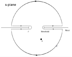
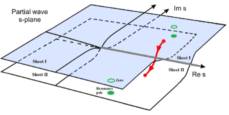
   Figure 1: Left: Analytic structure in the $s$-plane for fixed-$t$. Right: Two-sheet structure for elastic partial waves. Poles appear in the second sheet. In the same location a zero appears in the $S$-matrix.

   Dispersion relations are useful for calculating the amplitude where there is no data, to constrain data analyses or to look for resonance poles in the complex plane. Actually, the rigorous mathematical definition of a resonance involves the existence of a pair of conjugated poles in the second Riemann sheet of a partial wave amplitude. This sheet is reached by crossing continuously the physical cut, as seen on the right side of Figure 1. The position of the pole in the lower half plane is related to the mass $M$ and with $\Gamma$ of the resonance as $\sqrt{s_{pole}}=M-i\Gamma/2$.

   So far we have discussed the physical cut and its sheet structure, but in Figure 2 we show the complicated analytic structure of $\pi K$ scattering partial waves, which includes the "unphysical" left cut and an additional circular cut which appears due to the different pion and kaon masses. Now, when the pole of a resonance is far from other singularities and close to the real axis, namely $\Gamma<<M$, as it is the case of the $K^{\ast}(892)$, whose width is $\sim 50\,$MeV, it is seen in the real axis, i.e., experimentally, as a peak in the amplitude. Simple parameterizations of data just around its nominal mass, like a Breit-Wigner formula, can describe such resonances rather well. However, for very wide resonances like the $\kappa/K^{\ast}_{0}(800)$, the energy region around its nominal mass is more distant than other energy regions and particularly the threshold region. This threshold will distort dramatically the peak naively expected for a resonance. In addition, chiral symmetry implies the existence of the so-called Adler zero below threshold, which once again is close to the pole ans distorts its simple shape when seen at physical energies. Finally, the nominal mass region is also at a comparable distance to the pole as the circular cut and the left cut and their contributions should not be discarded a priori but should taken into account for precise pole determinations.

   Therefore, the $\kappa/K_{0}^{\ast}(800)$ resonance cannot be described with precision just by the knowledge of data around its nominal mass, and the pole cannot be extracted with simple formulas that do not posses the correct analytic structures or that do not have the correct low-energy constraints of the QCD spontaneous chiral symmetry breaking. This is the reason why dispersion relations and analyticity properties are relevant tools to analyze data and the use of simple models can lead to considerable confusion or artifacts. In addition, data in the near threshold region impose strong constraints to the pole position, even if the resonance is nominally at a higher mass. This partly explains the situation of the $\kappa/K^{\ast}_{0}(800)$ in the RPP where, as we will see in the final section, the poles obtained with Breit-Wigner formulas are quite spread and do not coincide with those obtained using more rigorous formalisms.

   

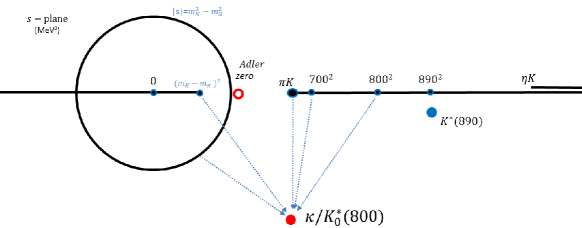
   Figure 2: Analytic structure of the $\pi K$ partial waves in the complex $s$-plane (in MeV²). Note the existence of a left cut up to $(m_{K}-m_{\pi})^{2}$ and a circular cut. We have shown the position of the poles associated to the $K^{\ast}(892)$ and the $\kappa/K^{\ast}_{0}(800)$.

   Note that in order to write Cauchy’s Theorem as we described above we need to consider the amplitude as a one-variable function. For this, there are two approaches:

   1. Fix one variable and obtain a dispersion relation in terms of the other. This leads to the popular fixed-$t$ dispersion relations, although one could also obtain fixed-$u$ or even fixed-$s$ dispersion relations. But one can also fix one variable in terms of the other one by means of a constrain. For instance, this is the case of Hiperbolic Dispersion Relations, where one imposes a constraint $(s-a)(u-a)=b$. Complicated relations like the latter are used to maximize the applicability region of the Dispersion Relation but if that is not needed for a particular study a simple choice could be more convenient. Of particular interest are Forward Dispersion Relations (FDRs), $t=0$, since they yield rather simple expressions and because the higher part of the integrals can be expressed in terms of total cross sections thanks to the Optical Theorem. These FDRs have also the advantage that they can be applied in principle up to arbitrarily high energies and that their analytic structure is very simple. This makes it easier to use crossing symmetry in order to rewrite the left-cut contributions in terms of physical amplitudes over the physical cut. Their expressions are rather simple for $\pi K$ scattering and as we will see below provide stringent constraints on the description of existing data. Unfortunately it is not possible to use the integral FDRs to access the second Riemann sheet in search for poles.

   2. Partial-wave Dispersion Relations. Now the scattering angle dependence is eliminated by projecting the amplitudes in partial waves, $t_{J}(s)$. The main advantage is that the second Riemann sheet, where resonance poles can appear, is easily accessible. The reason is that, due to unitarity, for elastic partial waves the second Riemann sheet of the $S$ matrix is just the inverse of the first, namely $S_{J}^{II}(s)=1/S^{I}_{J}(s)$. Recalling that $S_{J}(s)=1-2i\sigma(s)t_{J}(s)$ with $\sigma(s)=k/2\sqrt{s}$, where $k$ is the CM-momentum, then the Second Riemann Sheet partial wave amplitude can be obtained from the first as follows:

      $$t_{J}^{II}(s)=\frac{t_{J}^{I}(s)}{1-2i\sigma(s)t_{J}^{I}(s)}$$ (1)

      Unfortunately, when the scattering particles do not have equal masses, the partial-wave projection leads to a more complicated analytic structure. For $\pi K$ partial waves this structure was already shown in Fig. 2 and includes a new circular cut and a longer left cut. The most difficult part of using Dispersion Relation is to calculate the contributions along these unphysical cuts, and two main approaches appear once again in the literature:

      1. Do not use crossing and just approximate the left cut. This leads to simple dispersion relations (see for instance [2]) and has become very popular when combined with Chiral Perturbation Theory to approximate the left cut and the subtraction constants. Within this approach, the dispersion relations are written for the inverse partial-wave, since unitarity fixes its imaginary part in the elastic region. This approach is known as the Inverse Amplitude Method [3] that is one instance of Unitarized Chiral Perturbation Theory. It provides a fairly good description of data and yields the poles of all resonances that appear in the two-body scattering of pions and kaons below 1 GeV. In particular, a pole for the kappa is found at [4] $(753\pm 52)-i(235\pm 33)\,$MeV. Despite not being good for precision, it is very convenient to connect the meson scattering phenomenology with QCD parameters like $N_{c}$ or the quark masses [5] and thus study the nature of resonances.

      2. Use crossing to rewrite the contributions from unphysical cuts in terms of Use crossing to rewrite the contributions from unphysical cuts in terms of partial waves on the physical cut. Unfortunately, when projecting into a partial wave of the $s$-angle, one does not extract a single partial wave in the $u$-channel angle, so that the whole tower of partial waves is still present when rewriting the unphysical cuts into the physical region using crossing. This leads to an infinite set of coupled dispersion relations. These are called Roy-Steiner dispersion relations [6] (different versions can be obtained starting from fixed-$t$ or hyperbolic dispersion relations). They are more cumbersome to use, and usually they are applied only to the lowest partial waves, taking the rest as fixed input. However, they yield the most rigorous determination of the $\kappa/K_{0}^{\ast}(800)$ pole so far [7]: $(658\pm 13)-i(278.5\pm 12)\,$MeV. Note that in these works Roy-Steiner equations were solved in the elastic region for the $S$ and $P$ waves, using data on higher energies and higher waves as input, but no data on the elastic region below $\sim$1 GeV. It was also shown that the pole appears within the Lehman-ellipse that ensures the convergence of the partial-wave expansion (actually, even inside a more restrictive region that also ensures the use of hyperbolic dispersion relations). Nevertheless the RPP still considers that the existence of the $\kappa/K_{0}^{\ast}(800)$ “ Needs Confirmation”.

   3. Amplitudes Constrained with Forward Dispersion Relations

      Hence, in order to provide the required confirmation of the $\kappa/K_{0}^{\ast}(800)$ existence and of the values of its parameters, we have recently performed a Forward Dispersion Relation study of $\pi K$ scattering data [8]. The explicit expressions of the FDRs for the symmetric amplitude $T^{+}$ and the antisymmetric one $T^{-}$ and all other details can be found in [8]. We took particular care to use simple parameterizations of data on partial waves that could be easily used later in further theoretical or experimental studies. The first relevant result, as shown in the left column of Fig. 3 is that the

      Unconstrained Fits to Data (UFD) do not satisfy FDRs well, particularly at high energies and in the threshold region.

      

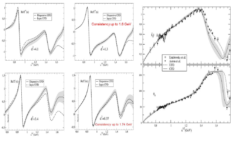
      Figure 3: Left Column: The input from Unconstrained Fits to Data (UFD) do not agree well with the Dispersive output of FDRs. Central Column: By imposing FDRs as constraints on data fits (CFD) they can be well satisfied up to 1.6 GeV without spoiling the data description. Right Column: The difference between UFD and CFD data descriptions. Data comes from Ref. [9].

      For this reason we imposed the FDRs to obtain Constrained Fits to Data (CFD). Once this is done the agreement is remarkable up to 1.6 GeV for the symmetric FDR and up to 1.74 GeV for the antisymmetric one, as seen in the central column of Fig. 3. In the right column of that figure, we show that the difference between the UFD and CFD is significant above 1.4 GeV and also in the threshold region for the phase, where there is very little experimental information. As we have already commented when discussing the $\kappa$ pole and Fig.2, this area is particularly relevant for the determination of the $\kappa/K_{0}^{\ast}(800)$ resonance from experimental data. It would be very interesting to have new data to confirm our findings and this could certainly be achieved with the proposed kaon beam at JLab.

      Moreover, it can be seen in that last column of Fig.2, that the most reliable data source, which is coming from the LASS/SLAC spectrometer [9], only provides a combination of isospins, but not the separated $I=1/2$ and $I=3/2$ partial waves. Actually, the information on $I=3/2$ is rather scarce and sometimes contradictory [9]. This will be one of the main sources of uncertainty in our calculation of the $\kappa$ pole. As it has already been explained in other talks of this conference that a clear isospin separation could be achieved with the proposed kaon beam facility.

   4. Analytic Methods to Extract Resonances

      Our parameterizations of the data are obtained from piece-wise analytic functions which are carefully matched to impose continuity. Therefore, none of the pieces by itself has all the relevant information to determine the resonance poles with precision. Nevertheless, the lowest energy piece was constructed by means of a conformal expansion, which exploits the analyticity of the partial wave on the full complex plane and has the correct analytic structure while satisfying the elastic unitarity constraint that allows for a continuation to the second Riemann sheet as explained in Eq. 1. We have actually checked that this simple parameterization yields a pole for the $\kappa/K_{0}^{\ast}(800)$ at: $(680\pm 15)-i(334\pm 7.5)$. However, this still makes use of a specific parameterization and, no matter how good it might be, is still model-dependent and the small uncertainties can only be understood within that model.

      However, there is a procedure to extract poles [10], which is model independent in the sense that it does not rely on a specific parameterization choice. It is based on a powerful theorem of Complex Analysis, which ensures that in a given domain where a function is analytic except for a pole, one can construct a sequence of Padé approximants that contains a pole that converges to the actual pole in the function. This sequence is built in terms of the values of the partial wave and the derivatives at a given point within that domain. Thus, using our amplitudes constrained with FDRs (CFD), we have searched [11] for a point in the real axis in which we can define a domain that includes the expected $\kappa/K_{0}^{\ast}(800)$ pole and built a sequence of Padés. In this way we have confirmed the existence of the $\kappa/K_{0}^{\ast}(800)$ pole [11] and its location at: $(670\pm 18)-i(295\pm 28)$. This time the errors are larger because the determination does not depend on a specific parameterization. Similar results have been obtained for all the resonances that appear in $\pi K$ scattering below 1.8 GeV (except for the $K^{\ast}(1680)$), thus providing further support for their existence and a determination of their parameters that do not depend on approximations or specific choices of parameterizations like Breit-Wigner parameterizations. Further details can be found in [11].

      Of course, the best would be a new analysis of the Roy-Steiner type, independent from that of [7]. Actually our Madrid group already has a preliminary result of this kind of analysis which finds a pole at $(662\pm 13)-i(289\pm 25)\,$MeV [12]. For this we use partial-wave Roy-Steiner-like equations obtained from hyperbolic dispersion relation using as input the amplitudes constrained to satisfy FDRs [8], and therefore using data below 1 GeV instead of solving the equations in the elastic region as in Ref [7]. We are showing this preliminary result in red in Fig. 4, together with all the other poles mentioned in this mini-review.

      Note however that there is considerable room for improvement by reducing the uncertainties. For this it would be of the uttermost importance not only to have more precise data, but also data in the regions where there is none nowadays, and particularly with a clear separation of partial waves with different isospin. As we have seen in this workshop, all this could be achievable with the proposed kaon beam at JLab that therefore could provide a sound experimental basis for the understanding of the spectroscopy of strange mesons, which nowadays relies on strong model-dependent assumptions and data sets with strong inconsistencies among themselves and with the fundamental dispersive constraints.

      

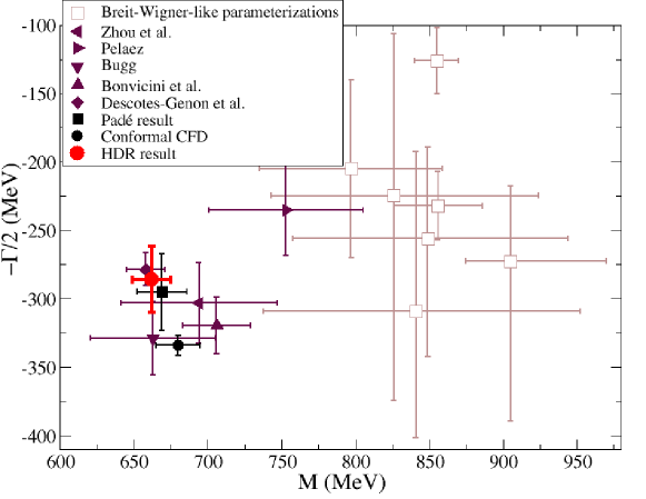
      Figure 4: Compilation of results for the $\kappa/K^{\ast}_{0}(800)$ resonance pole positions. We list as empty squares all the determinations using some for of Breit-Wigner shape listed in the RPP [PDG]. The rest of references correspond to: Zhou et al. [2], Pelaez [4], Bugg [13], Bomvicini [14], Descotes-Genon et al. [7], Padé result [11], Conformal CFD [8] and our preliminary HDR result using Roy-Steiner equations [12]

3. Acknowledgments

   JRP and AR are supported by the Spanish Project FPA2016-75654-C2-2-P. The work of JRE was supported by the Swiss National Science Foundation. AR would also like to acknowledge financial support of the Universidad Complutense de Madrid through a predoctoral scholarship.

3.15 Analyticity Constraints for Exotic Mesons

Vincent Mathieu

Thomas Jefferson National Accelerator Facility

Newport News, VA 23606, U.S.A.

1. Introduction

   Despite the knowledge of the Quantum ChromoDynamics (QCD) Lagrangian for about 50 years and the abundance of data, the pole position of the lowest QCD resonances, the $\sigma$ and $\kappa$ mesons also called $f_{0}(500)$ and $K^{\ast}_{0}(800)$ respectively, have remained inaccurate for decades. The situation of the $\sigma$ has, however, changed recently. The combined use of dispersion relations, crossing symmetry and experimental data have led independent teams to a precise location of the complex pole [1, 2, 3]. The interested readers can find a historical and technical review in Ref. [4].

   The situation of the $\kappa$ is going in the same direction. A recent analysis [5] using dispersion relation and crossing symmetry have determined its pole location accurately. Nevertheless, the lowest resonance with strangeness is currently not reported in the summary tables in the Review of Particle Properties [6]. This situation might change when the results of Ref. [5] will be confirmed independently. Studies in this direction are in progress [7].

   With these recent confirmation of existence and precise location of the $\sigma$ and $\kappa$ poles, the next challenge in meson spectroscopy is the existence of exotic mesons. The theoretical and experimental works tend to support the existence of an isovector with the quantum numbers $J^{PC}=1^{-+}$, denoted $\pi_{1}$, around 1400-1600 MeV. The experimental status is still nevertheless controversial [8]. As in the case of the $\sigma$ and the $\kappa$ meson, the (possible) large width of the $\pi_{1}$ prevents the use of standard partial-wave parametrizations, such as the Breit-Wigner formula, to extract the pole location. The parametrization of the exotic wave can, nevertheless, be constrained thanks to dispersive techniques.

   Dispersion relations, in meson-meson scatterings, are typically used in their subtracted form to reduce the influence of the, mostly unknown, high energy part. One can alternatively write dispersion relations for moments of the amplitudes. Using a Regge form for the high energy part, they lead to the finite energy sum rules (FESR) [9, 10]. FESR were applied recently in hadro- and photo-production on a nucleon target [11, 12, 13] in which data in the low and high energy mass region are available. With the advent of high statistic generation of hadron spectroscopy meson, one now has access to data in a wide energy range in meson-meson interaction. The COMPASS collaboration has reported $\pi\eta$ and $\pi\eta^{\prime}$ (acceptance corrected) partial waves from threshold to 3 GeV and has recorded data up to 5 GeV [14]. CLAS12 and GlueX are currently taking data on two mesons photo- and electro-production with an expected coverage up to at least 3 GeV. These data sets allow then to constrain the resonance region with the Regge region via FESR.

   Schwimmer [15] has demonstrated that duality and the non-existence of odd wave in elastic $\pi\eta$ scattering lead to a degeneracy relation between Regge exchange residues in the equal mass case. In order words, in the equal mass case, the equality between the forward and backward region at high energy is equivalent to the non-existence of odd waves. This results, showing the self-consistency of the quark model, was actually already included in the general results of Mandula, Weyers and Zweig [16] also in the $SU(3)$ symmetry limit.

   Here I demonstrate how FESR in elastic $\pi\eta$ scattering can be used to constrain the exotic $P$-wave. I examine Schwimmer argument with exact kinematics and derive the forward and backward FESR for $\pi\eta$ scattering. It is shown how the deviation from forward/backward equality and the mass difference is related to the amount of exotic meson in $\pi\eta$ scattering.

   The kinematics are reviewed in Section 2 and the FESR are written in Section 3. The main results are derived in Section 4.

2. Kinematics

   

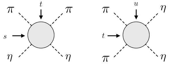
   Figure 1: The $s$-channel $\pi\eta\to\pi\eta$ and the $t$-channel $\pi\pi\to\eta\eta$.

   The $s-$channel reaction $\pi\eta\to\pi\eta$. The $u-$channel is identical to the $s-$channel and the $t-$channel is $\pi\pi\to\eta\eta$, as depicted in Fig 1. All channels are described by a single function $A(s,t,u)$. Let $m_{\pi}$ and $m_{\eta}$ be the masses of the $\pi$ and $\eta$ mesons, and $s+t+u=\Sigma=2m_{\pi}^{2}+2m_{\eta}^{2}$. The center-of-mass momentum and scattering angle in the $s$-channel are

   $$q^{2} =\frac{1}{4s}\left(s-(m_{\pi}+m_{\eta})^{2}\right)\left(s-(m_{\pi}-m_{\eta})^{2}\right),$$ (1a)

   $$z_{s} =1+\frac{t}{2q^{2}}=-1-\frac{u-u_{0}}{2q^{2}}, u_{0} =\frac{(m_{\eta}^{2}-m_{\pi}^{2})^{2}}{s}$$ (1b)

   The unitarity threshold of the $s$- and $u$-channels is $(m_{\pi}+m_{\eta})^{2}$. In the $t$-channel the threshold is $4m_{\pi}^{2}$. I will do fixed-$t$ and fixed-$u$ dispersion relations and finite energy sum rules. Fixed-$s$ sum rules are identical to fixed-$u$ sum rules. The crossing variables are $\nu=(s-u)/2$ and $\nu^{\prime}=(s-t+4m_{\pi}^{2}-(m_{\eta}+m_{\pi})^{2})/2$. $\nu^{\prime}$ is designed to symmetrize the two cuts at fixed $u$, i.e., $\nu^{\prime}(s=(m_{\eta}+m_{\pi})^{2})=-\nu^{\prime}(t=4m_{\pi}^{2})$. That will allow to place both cuts under the same integral in the fixed-$u$ sum rules. I will need to trade the Mandelstam variables for the pair $(\nu,t)$ and $(\nu^{\prime},u)$ via

   $$s(\nu,t) =+\nu-(t-\Sigma)/2, s(\nu^{\prime},u) =+\nu^{\prime}-(u-4m_{\eta}^{2}+(m_{\eta}-m_{\pi})^{2})/2,$$ (2a)

   $$u(\nu,t) =-\nu-(t-\Sigma)/2, t(\nu^{\prime},u) =-\nu^{\prime}-(u-4m_{\pi}^{2}-(m_{\eta}-m_{\pi})^{2})/2,$$ (2b)

   so that $s(-\nu,t)=u(\nu,t)$.

3. Finite Energy Sum Rules

   

   

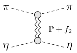
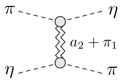
   Figure 2: Exchanges in forward (left) and backward (right) $\pi\eta$ elastic scattering.

   I consider small $t=x$, i.e., small angles with the pion going forward. The two exchanges at high energy are the Pomeron and the $f_{2}$ Regge pole. At high energy, the Regge form is $\operatorname{Im}A(s,t,u)=\beta_{\mathbb{P}}(t)\nu^{\alpha_{\mathbb{P}}}+\beta_{f_{2}}(t)\nu^{\alpha_{f_{2}}}$ for $\nu>\Lambda$. The threshold is $\nu_{0}(x)=2m_{\eta}m_{\pi}+x/2$. The FESR at fixed $t$ reads

   $$\int_{\nu_{0}(t)}^{\Lambda}\operatorname{Im}\left\{A\left[s(\nu,x),x,u(\nu,x)\right]+(-)^{k}A\left[s(-\nu,x),x,u(-\nu,x)\right]\right\}\nu^{k}d\nu$$

   $$=\sum_{\tau}\left[1+\tau(-)^{k}\right]\beta_{\tau}(t)\frac{\Lambda^{\alpha_{\tau}(t)+k+1}}{\alpha_{\tau}(t)+k+1}$$ (3)

   The $s$- and $u$-channel are identical, so $A(s,x,u)=A(u,x,s)$ and there can only be even moments. This is consistent with the exchanges that can only have positive signature $\tau(\mathbb{P})=\tau(f_{2})=+1$. I obtain, with $n$ a positive integer

   $$\int_{\nu_{0}(x)}^{\Lambda}\operatorname{Im}A\left[s(\nu,x),x,u(\nu,x)\right]\nu^{2n}d\nu =\beta_{\mathbb{P}}(x)\frac{\Lambda^{\alpha_{\mathbb{P}}(x)+2n+1}}{\alpha_{\mathbb{P}}(x)+2n+1}+\beta_{f}(x)\frac{\Lambda^{\alpha_{f_{2}}(x)+2n+1}}{\alpha_{f_{2}}(x)+2n+1}$$ (4)

   The factorization of Regge pole allow write $\beta_{\mathbb{P}}(x)=\beta^{\pi\pi}_{\mathbb{P}}(x)\beta^{\eta\eta}_{\mathbb{P}}(x)$ and $\beta_{f}(x)\equiv\beta^{\pi\pi}_{f_{2}}(x)\beta^{\eta\eta}_{f_{2}}(x)$, as represented in Fig. 2.

   I now consider small $u=x$, i.e., small angles with the eta meson going forward. The threshold is $\nu^{\prime}_{0}(x)=(4m_{\pi}^{2}-(m_{\eta}-m_{\pi})^{2}+x)/2$. Similarly to the fixed-$t$ case, the FESR at fixed $u$ read

   $$\int_{\nu^{\prime}_{0}(x)}^{\bar{\Lambda}}\operatorname{Im}\left\{A\left[s(\nu^{\prime},x),t(\nu^{\prime},x),x\right]+(-)^{k}A\left[s(-\nu^{\prime},x),t(-\nu^{\prime},x),x\right]\right\}\nu^{\prime k}d\nu^{\prime}$$

   $$=\sum_{\tau}\left[1+\tau(-)^{k}\right]\beta_{\tau}(x)\frac{\bar{\Lambda}^{\alpha_{\tau}(x)+k+1}}{\alpha_{\tau}(x)+k+1}$$ (5)

   There are two kinds of exchanges. The positive signature $a_{2}$ pole and the negative signature $\pi_{1}$ pole. So for $k$ even there is the $a_{2}$ pole and $k$ odd the $\pi_{1}$ (exotic) pole. I thus obtain two backward FESR:

   $$\frac{1}{2}\int_{\nu^{\prime}_{0}(x)}^{\bar{\Lambda}}\operatorname{Im}\left\{A\left[s(\nu^{\prime},x),t(\nu^{\prime},x),x\right]+A\left[s(-\nu^{\prime},x),t(-\nu^{\prime},x),x\right]\right\}\nu^{\prime 2n}d\nu^{\prime} =\frac{\beta_{a_{2}}(x)\bar{\Lambda}^{\alpha_{a_{2}}(x)+2n+1}}{\alpha_{a_{2}}(x)+2n+1}$$

   $$\frac{1}{2}\int_{\nu^{\prime}_{0}(x)}^{\bar{\Lambda}}\operatorname{Im}\left\{A\left[s(\nu^{\prime},x),t(\nu^{\prime},x),x\right]-A\left[s(-\nu^{\prime},x),t(-\nu^{\prime},x),x\right]\right\}\nu^{\prime 2n+1}d\nu^{\prime} =\frac{\beta_{\pi_{1}}(x)\bar{\Lambda}^{\alpha_{\pi_{1}}(x)+2n+2}}{\alpha_{\pi_{1}}(x)+2n+2}$$ (6)

   Again, the factorization of Regge pole leads to $\beta_{a_{2}}(x)=\left[\beta^{\pi\eta}_{a_{2}}(x)\right]^{2}$ and $\beta_{\pi_{1}}(x)=\left[\beta^{\pi\eta}_{\pi_{1}}(x)\right]^{2}$ as displayed in Fig. 2. For small $x$, the amplitude $A\left[s(\nu^{\prime},x),t(\nu^{\prime},x),x\right]$ represents the reaction $\pi\eta\to\pi\eta$ in the backward direction and $A\left[s(-\nu^{\prime},x),t(-\nu^{\prime},x),x\right]$ represents the $t$-channel reaction $\pi\pi\to\eta\eta$.

4. Constraint on Exotica Production

   Several models are available for the elastic $\pi\eta$ $S$-wave [17, 18, 19, 20]. For higher waves, little information is known beside the resonance content. The elastic $\pi\eta$ $D$-wave is certainly dominated by the $a_{2}(1320)$ meson. At higher mass, the excitation $a_{2}^{\prime}(1700)$ has been recently confirm by a joint publication by the JPAC and COMPASS collaborations [21], but its branching fraction to $\pi\eta$ is not known. The branching ratio of the $a_{4}(2040)$ is not known either but quark model calculations yields the width $\Gamma(a_{4}\to\pi\eta)\sim(1.7-2.4)^{2}$ MeV [22, 23].

   Experimental information on $\pi\pi\to\eta\eta$ are available above the $\eta\eta$ threshold [Binon:1983ny]. Below the physical threshold, one can use Watson’s theorem and the $\pi\pi$ elastic phase shift from the unitarity threshold up to the $K\bar{K}$ threshold. Unfortunately between the $K\bar{K}$ and the $\eta\eta$ thresholds, little information is known about the phase shift and inelasticities of the $\pi\pi\to\eta\eta$ amplitude. Although some couple channels calculations exist, see for instance [25].

   The $a_{2}$, $f_{2}$ are lying on the trajectory degenerate with the $\rho$ and $\omega$ one with $\alpha_{a_{2}}(t)=\alpha_{f_{2}}(t)\equiv\alpha_{N}(t)\sim 0.9t+0.5$. The exotic $\pi_{1}$ is lying on a trajectory below the leading natural exchange trajectory. A mass around 1.6 GeV yields the intercept $\alpha_{\pi_{1}}(0)\sim\alpha_{N}(t)-1$, which makes both right-hand-side of Eq. (6) for the same $n$ of the same order up to the residues $\beta_{a_{2}}$ and $\beta_{\pi_{1}}$. The existence of an exotic would make $\beta_{\pi_{1}}$ not zero. However since its pole would be far away from the physical region, there is a possibility of $\beta_{\pi_{1}}(x)$ (with $x<0$) being small. In this case, one could neglect the right-hand-side of the second sum rule in Eq. (6) for any $n$, which would lead to

   $$\operatorname{Im}A\left[s(\nu^{\prime},x),t(\nu^{\prime},x),x\right]\approx\operatorname{Im}A\left[s(-\nu^{\prime},x),t(-\nu^{\prime},x),x\right]$$ (7)

   Using this approximation, I can subtract the forward $t=x$ and backward $u=x$ sum rules to obtain the constraint

   $$\int_{\nu_{0}(x)}^{\Lambda}\operatorname{Im}\left\{A\left[s(\nu,x),x,u(\nu,x)\right]-A\left[s(\nu,x),t(\nu,x),x\right]\right\}\nu^{2n}\mathrm{d}\nu=$$

   $$\beta_{\mathbb{P}}(x)\frac{\Lambda^{\alpha_{\mathbb{P}}(x)+2n+1}}{\alpha_{\mathbb{P}}(x)+2n+1}+\left[\beta_{f_{2}}(x)-\beta_{a_{2}}(x)\right]\frac{\Lambda^{\alpha_{N}(x)+2n+1}}{\alpha_{N}(x)+2n+1}$$ (8)

   In term of partial waves, the forward and backward amplitudes read

   $$A\left(s,x,u\right) =\sum_{\ell}(2\ell+1)t_{\ell}(s)P_{\ell}(z_{1}), z_{1} =+1+\frac{x}{2q^{2}},$$ (9a)

   $$A\left(s,t,x\right) =\sum_{\ell}(2\ell+1)t_{\ell}(s)P_{\ell}(z_{2}), z_{2} =-1-\frac{x-u_{0}}{2q^{2}},$$ (9b)

   with $q$ and $u_{0}$ evaluated at $s(\nu,x)$. If the forward and backward direction were exactly equal, i.e., $u_{0}=0$ the even waves would exactly cancel in Eq. (8). The reader can then see that the two components duality and the absence of odd wave would then imply degeneracy between the $f_{2}$ and $a_{2}$ Regge exchanges as demonstrated by Schwimmer [15]. In the presence of only one odd wave $\ell=1$, its absorptive part is constrained by

   $$3\int_{\nu_{0}(x)}^{\Lambda}\operatorname{Im}t_{1}\left[s(\nu,x)\right]\left[P_{1}(z_{1})-P_{1}(z_{2})\right]\nu^{2n}d\nu =\beta_{\mathbb{P}}(x)\frac{\Lambda^{\alpha_{\mathbb{P}}(x)+2n+1}}{\alpha_{\mathbb{P}}(x)+2n+1}$$

   $$+\left[\beta_{f_{2}}(x)-\beta_{a_{2}}(x)\right]\frac{\Lambda^{\alpha_{N}(x)+2n+1}}{\alpha_{N}(x)+2n+1}$$

   $$-\sum_{\ell\in\text{even}}\int_{\nu_{0}(x)}^{\Lambda}\operatorname{Im}t_{\ell}(s_{\nu})\Delta_{\ell}(\nu,x)\nu^{2n}d\nu$$ (10)

   The even waves enter via the quantity $\Delta_{\ell}(\nu,x)=(2\ell+1)\left[P_{\ell}(z_{1})-P_{\ell}(z_{2})\right]$. Note that $\Delta_{\ell}\propto u_{0}$ (for $\ell$ even) vanishes in the limit $m_{\eta}\to m_{\pi}$. Of course the $S$-wave cancels $\Delta_{0}=0$. We also have $\frac{1}{2}\left[P_{1}(z_{1})-P_{1}(z_{2})\right]=1+x/2q^{2}-u_{0}/4q^{2}$. The individual contribution of the right-hand-side of Eq. (10) can be evaluated.

5. Acknowledgments

   I thank M. Albaladejo, A. Jackura, and J. Ruiz de Elvira for providing their elastic $\pi\eta$ solutions. This work was supported by the U.S. Department of Energy under grants No. DE-AC05-06OR23177

3.16 Pion–Kaon Final-State Interactions in Heavy-Meson Decays

Bastian Kubis and Franz Niecknig

Helmholtz-Institut für Strahlen- und Kernphysik (Theorie) and

Bethe Center for Theoretical Physics

Universität Bonn

53115 Bonn, Germany

1. What’s not to Like about the Isobar Model?

   In experimental analyses, the Dalitz-plot distributions of hadronic three-body decays are still conventionally described in terms of the isobar model: amplitudes are constructed in terms of subsequent two-body decays, and the resonant intermediate states mostly modeled in terms of Breit–Wigner line shapes. This is problematic in several respects. First of all, many resonances cannot be described by Breit–Wigner functions at all, be it due to the close proximity of thresholds (e.g., the $f_{0}(980)$ or the $a_{0}(980)$ among the light mesons, and many of the newly found, potentially exotic states in the charmonium and bottomonium sectors), or because their poles lie too far in the complex plane: prime examples include the lightest scalar resonances, the $f_{0}(500)$ or $\sigma$ (see the comprehensive review [1] and references therein) as well as, in the strange sector, the $K_{0}^{\ast}(800)$ [2, 3]. These problems can be avoided by using known phase shifts as input, potentially including coupled channels; see, e.g., Refs. [4, 5] for recent applications in the context of heavy-meson decays. On the other hand, models of subsequent two-body decays ignore rescattering effects between all three strongly interacting particles in the final state, which will in general affect the phase motion of the amplitudes in question. Close control over the various amplitude phases is, e.g., important in the context of CP-violation studies: rapidly varying, resonant strong phases may significantly enhance small weak phases (originating in the Cabibbo–Kobayashi–Maskawa matrix) locally in the Dalitz plot, which may give the search for CP violation in three-body charmed-meson decays the edge over two-body decays, which occur at fixed energy.

   A tool to consistently treat full iterated two-body final-state interactions in three-body decays are the so-called Khuri–Treiman equations [6], originally derived for the description of $K\to 3\pi$, and recently increasingly popular for the description of various low-energy decays such as $\eta\to 3\pi$ [7, 8, 9, 10, 11, 12], $\eta^{\prime}\to\eta\pi\pi$ [13], or $\omega/\phi\to 3\pi$ [14, 15]. We will illustrate the formalism with the last example in the following, before turning to the application in the more complex Dalitz plot studies of $D^{+}\to\bar{K}\pi\pi^{+}$ [16, 17].

2. Dispersion Relations for Three-Body Decays (1): $V\to 3\pi$

   Particularly simple examples of three-body decays are those of isoscalar vector mesons into three pions, $V\to 3\pi$, $V=\omega,\,\phi$. Pairs of pions can only be in odd relative partial waves; neglecting discontinuities in $F$- and higher partial waves, the decay amplitude can be decomposed into single-variable functions according to

   $$\mathcal{M}(s,t,u)=i\epsilon_{\mu\nu\alpha\beta}\,\epsilon_{V}^{\mu}p_{\pi^{+}}^{\nu}p_{\pi^{-}}^{\alpha}p_{\pi^{0}}^{\beta}\big{\{}\mathcal{F}(s)+\mathcal{F}(t)+\mathcal{F}(u)\big{\}},$$ (1)

   where $\epsilon_{V}^{\mu}$ denotes the vector meson’s polarization vector. The function $\mathcal{F}(s)$ obeys a discontinuity equation [14, 18]

   $$\mathrm{disc}\,\mathcal{F}(s) =2i\big{[}\mathcal{F}(s)+\hat{\mathcal{F}}(s)\big{]}\theta\big{(}s-4M_{\pi}^{2}\big{)}\sin\delta(s)e^{-\delta(s)},$$

   $$\hat{\mathcal{F}}(s) =\frac{3}{2}\int_{-1}^{1}\mathrm{d}z\big{(}1-z^{2}\big{)}\mathcal{F}\big{(}t(s,z)\big{)},$$ (2)

   where $z=\cos\theta_{s}$ denotes the cosine of the $s$-channel scattering angle, and $\delta(s)\equiv\delta_{1}^{1}(s)$ is the isospin $I=1$ $P$-wave $\pi\pi$ scattering phase shift. Without the inhomogeneity $\hat{\mathcal{F}}(s)$ in the discontinuity equation, the latter’s solution could be given in terms of an Omnès function [19] like a simple form factor, and the phase of $\mathcal{F}(s)$ would immediately coincide with $\delta(s)$ according to Watson’s theorem [20].

   

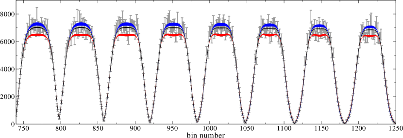
   Figure 1: Selected slices through the $\phi\to 3\pi$ Dalitz plot measured by the KLOE Collaboration [21], compared to the theoretical description of Ref. [14]. The fit with Omnès functions only, neglecting crossed-channel rescattering, is shown in red, once-subtracted Khuri–Treiman amplitudes in blue, and twice-subtracted Khuri–Treiman solutions in black. The widths of the uncertainty bands are due to variation of the phase shift input as well as fit uncertainties.

   The presence of the partial-wave-projected crossed-channel contributions $\hat{\mathcal{F}}(s)$ renders the solution of Eq. (2) slightly more complicated; it is given as

   $$\mathcal{F}(s)=\Omega(s)\biggl{\{}a+\frac{s}{\pi}\int_{4M_{\pi}^{2}}^{\infty}\frac{\mathrm{d}x}{x}\frac{\sin\delta(x)\hat{\mathcal{F}}(x)}{|\Omega(x)|(x-s)}\biggr{\}},\quad\Omega(s)=\exp\bigg{\{}\frac{s}{\pi}\int_{4M_{\pi}^{2}}^{\infty}\frac{\mathrm{d}x}{x}\frac{\delta(x)}{x-s}\bigg{\}},$$ (3)

   where $\Omega(s)$ is the Omnès function, and $a$ a subtraction constant that has to be fixed phenomenologically. Care has to be taken in performing the angular integral for $\hat{\mathcal{F}}(s)$ in Eq. (2) as to avoid crossing the right-hand cut: in decay kinematics, $\hat{\mathcal{F}}(s)$ itself becomes complex, signaling the appearance of three-particle cuts, and a simple phase relation between $\mathcal{F}(s)$ and the elastic scattering phase shift is lost.

   The solution to Eq. (3) is compared to high-statistics Dalitz plot data for $\phi\to 3\pi$ by the KLOE collaboration [21] in Fig. 1. Different $\pi\pi$ phases have been employed, derived from Roy (and similar) equations [22, 23]. Non-trivial, crossed-channel rescattering effects improve the data description significantly; introducing a second subtraction constant in order to better suppress imperfectly known high-energy behavior of the dispersion integral leads to a perfect fit [14]. A first modern experimental investigation of the $\omega\to 3\pi$ Dalitz plot by WASA-at-COSY [24] is not yet accurate enough to discriminate these subtle rescattering effects.

   

   

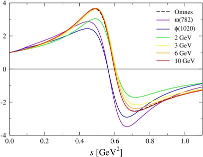
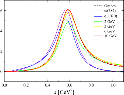
   Figure 2: Real (left) and imaginary (right) parts of single-variable amplitudes $\mathcal{F}(s)$ for varying decay masses, compared to the Omnès function.

   It is also interesting to investigate the dependence of $\mathcal{F}(s)$ on the decay mass: it differs for $\omega$ and $\phi$ decays [14, 15], but even has a well-defined high-energy limit, as shown in Fig. 2. For high decay masses, $\mathcal{F}(s)$ approaches the input Omnès function, i.e., crossed-channel rescattering effects vanish [25]. This conforms with physical intuition: if the third pion has a very large momentum relative to the other pair, its influence on the pairwise, resonant interaction should be small. Note that this limit is only formal, as inelastic effects as well as higher partial waves are not taken into account. Such a partial wave for variable and higher decay masses has been employed both for the description of the reaction $e^{+}e^{-}\to 3\pi$, which serves as an input for a dispersive analysis of the $\pi^{0}$ transition form factor [26], and in a study of the $J/\psi\to\pi^{0}\gamma^{\ast}$ transition form factor [27], in analogy to preceding studies of the conversion decays of the light vector mesons [28].

3. Dispersion Relations for Three-Body Decays (2): $D^{+}\to\bar{K}\pi\pi^{+}$

   In the first attempt to employ Khuri–Treiman equations to describe $D$-meson decays, we have chosen to consider the Cabibbo-favored processes $D^{+}\to K^{-}\pi^{+}\pi^{+}$ and $D^{+}\to\bar{K}^{0}\pi^{0}\pi^{+}$. The data situation for these is rather good, with high-statistics Dalitz plot measurements available by the E791 [29], CLEO [30], and FOCUS [31, 32] Collaborations for the fully charged final state, and more recently by BESIII for the partially neutral one [33]. Theoretical analyses of $D^{+}\to K^{-}\pi^{+}\pi^{+}$ have typically concentrated on improved descriptions of the $\pi K$ $S$-wave [34, 35, 36, 37, 38], however neglecting rescattering with the third decay particle. Ref. [39] is the only previous combined study of both decay channels, using Faddeev equations to generate three-body rescattering effects.

   An interesting aspect of these two decay channels is that they are coupled by a simple charge-exchange reaction, and can be related to each other by isospin; however, this relation is largely lost as long as only two-body rescattering is considered: e.g., the isospin $I=1$ $\pi\pi$ $P$-wave only features indirectly in the fully charged final state, where the $\rho(770)$ resonance can obviously not be observed. Otherwise, we truncate the partial-wave expansion consistently beyond $D$-waves, but among the exotic, non-resonant ones only retain the $S$-waves (the $I=2$ $\pi\pi$ and the $I=3/2$ $\pi K$ $S$-waves). This way, beyond the aforementioned $\rho(770)$, the following $\pi K$ resonances are included in the Dalitz plot description as the dominant structures: $K_{0}^{\ast}(800)$, $K_{0}^{\ast}(1430)$, $K^{\ast}(892)$, [$K^{\ast}(1410)$,] and $K_{2}^{\ast}(1430)$.

   The decomposition of the two decay amplitudes up-to-and-including $D$-waves has been derived [16] and proven in the sense of the reconstruction theorem [25]. With the exception of the $D$-wave, the number of subtractions has been determined by imposing the Froissart bound [40]; note that some of them can be eliminated consistently due to the constraint $s+t+u=\text{const.}$. The full system then reads

   $$\mathcal{F}_{0}^{2}(u) =\Omega^{2}_{0}(u)\frac{u^{2}}{\pi}\int_{u_{\mathrm{th}}}^{\infty}\frac{\mathrm{d}u^{\prime}}{u^{\prime 2}}\frac{\hat{\mathcal{F}}_{0}^{2}(u^{\prime})\sin\delta^{2}_{0}(u^{\prime})}{\left|\Omega^{2}_{0}(u^{\prime})\right|(u^{\prime}-u)},$$

   $$\mathcal{F}_{1}^{1}(u) =\Omega^{1}_{1}(u)\Bigg{\{}c_{0}+c_{1}u+\frac{u^{2}}{\pi}\int_{u_{\mathrm{th}}}^{\infty}\frac{\mathrm{d}u^{\prime}}{u^{\prime 2}}\frac{\hat{\mathcal{F}}_{1}^{1}(u^{\prime})\sin\delta^{1}_{1}(u^{\prime})}{\big{|}\Omega^{1}_{1}(u^{\prime})\big{|}(u^{\prime}-u)}\Bigg{\}},$$

   $$\mathcal{F}_{0}^{1/2}(s) =\Omega^{1/2}_{0}(s)\Bigg{\{}c_{2}+c_{3}s+c_{4}s^{2}+c_{5}s^{3}+\frac{s^{4}}{\pi}\int_{s_{\mathrm{th}}}^{\infty}\frac{\mathrm{d}s^{\prime}}{s^{\prime 4}}\frac{\hat{\mathcal{F}}_{0}^{1/2}(s^{\prime})\sin\delta^{1/2}_{0}(s^{\prime})}{\big{|}\Omega^{1/2}_{0}(s^{\prime})\big{|}(s^{\prime}-s)}\Bigg{\}},$$

   $$\mathcal{F}_{0}^{3/2}(s) =\Omega^{3/2}_{0}(s)\Bigg{\{}\frac{s^{2}}{\pi}\int_{s_{\mathrm{th}}}^{\infty}\frac{\mathrm{d}s^{\prime}}{s^{\prime 2}}\frac{\hat{\mathcal{F}}_{0}^{3/2}(s^{\prime})\sin\delta^{3/2}_{0}(s^{\prime})}{\big{|}\Omega^{3/2}_{0}(s^{\prime})\big{|}(s^{\prime}-s)}\Bigg{\}},$$

   $$\mathcal{F}_{1}^{1/2}(s) =\Omega^{1/2}_{1}(s)\Bigg{\{}c_{6}+\frac{s}{\pi}\int_{s_{\mathrm{th}}}^{\infty}\frac{\mathrm{d}s^{\prime}}{s^{\prime}}\frac{\hat{\mathcal{F}}_{1}^{1/2}(s^{\prime})\sin\delta^{1/2}_{1}(s^{\prime})}{\big{|}\Omega^{1/2}_{1}(s^{\prime})\big{|}(s^{\prime}-s)}\Bigg{\}},$$

   $$\mathcal{F}_{2}^{1/2}(s) =\Omega^{1/2}_{2}(s)\Bigg{\{}c_{7}+\frac{s}{\pi}\int_{s_{\mathrm{th}}}^{\infty}\frac{\mathrm{d}s^{\prime}}{s^{\prime}}\frac{\hat{\mathcal{F}}_{2}^{1/2}(s^{\prime})\sin\delta^{1/2}_{2}(s^{\prime})}{\big{|}\Omega^{1/2}_{2}(s^{\prime})\big{|}(s^{\prime}-s)}\Bigg{\}},$$ (4)

   where $s$ (and $t$) are the Mandelstam variables describing $\pi K$ invariant masses, while $u$ refers to the $\pi\pi$ system; the lower limits of the dispersion integrals are given by $s_{\mathrm{th}}=(M_{K}+M_{\pi})^{2}$ and $u_{\mathrm{th}}=4M_{\pi}^{2}$. Explicit formulae for the various $\hat{\mathcal{F}}_{L}^{I}$ are given in Ref. [16]. We have used the $\pi K$ phase shifts of Ref. [41] as input (note also other new [42] and ongoing [43] analyses of $\pi K$ scattering). Eq. (4) therefore contains 8 complex subtractions constants, which (subtracting one overall normalization and one overall phase) need to be fitted to data. In particular, the subtraction in $\mathcal{F}_{2}^{1/2}(s)$ was introduced a posteriori, as it turned out to be necessary to describe both Dalitz plots consistently [17]. As we work in the approximation of elastic unitarity, we refrain from describing the parts of the Dalitz plot for which $\sqrt{s},\,\sqrt{t}\geq M_{\eta^{\prime}}+M_{K}\approx 1.45\,\text{GeV}$, which is taken as the typical onset of significant inelasticities in particular in the $S$-wave. Note that no isoscalar $\pi\pi$ $S$-wave can contribute in these decays, with its sharp onset of inelasticities around the $f_{0}(980)$.

   

   Figure 3: Left: Moduli of single-variable amplitudes, in arbitrary units: CLEO/FOCUS fits (blue), BESIII (red), combined fit with improved $D$-wave (turquoise). Right: Phases of the single-variable amplitudes and input scattering phases (black) in radiant. The dashed lines visualize the fitted area: from threshold to the $\eta^{\prime}K$ threshold for the $\pi K$ amplitudes, the full phase space for the $\pi\pi$ amplitudes. Figure taken from Ref. [17].

   Moduli and phases of the resulting single-variable amplitudes $\mathcal{F}_{L}^{I}$ are shown in Fig. 3. Obviously, the different data sets constrain the various amplitudes differently: the $\pi\pi$ $P$-wave is only well constrained when including the BESIII data on the partially neutral final state (in which it features directly), while in contrast, the $\pi\pi$ $I=2$ $S$-wave is determined with much higher precision in the $K^{-}\pi^{+}\pi^{+}$ final state.

   	BESIII${}_{\text{combined}}$	CLEO/FOCUS${}_{\text{combined}}$
   $\text{FF}_{0}^{2}$	$(1.7\pm 0.5)\%$	$(5\pm 1)\%$
   $\text{FF}_{1}^{1}$	$(23\pm 3)\%$	—
   $\text{FF}_{0}^{1/2}$	$(36\pm 5)\%$	$(46\pm 6)\%$
   $\text{FF}_{1}^{1/2}$	$(8.5\pm 0.4)\%$	$(11.5\pm 0.5)\%$
   $\text{FF}_{0}^{3/2}$	$(6\pm 1)\%$	$(0.6\pm 0.1)\%$
   $\text{FF}_{2}^{1/2}$	$(0.5\pm 0.1)\%$	$(0.7\pm 0.1)\%$

   Table 1: Fit fractions of the various partial waves for the best combined fit. The errors are evaluated by varying the basis functions within their uncertainty bands. The fit fractions of the $\pi K$ amplitudes in the $s$- and $t$-channel are summed together.

   Given the relatively large number of subtraction constants compared to the $\phi\to 3\pi$ analysis described in the previous section, the necessity to include Khuri–Treiman amplitudes as opposed to simple polynomial-times-Omnès functions is demonstrated less by the best $\chi^{2}/\text{d.o.f.}$, but rather by the resulting fit fractions, which become implausibly large in particular for the nonresonant waves in the case of Omnès fits [16]. Similar observations are made when neglecting the $D$-wave. The fit fractions for the best combined fit to the CLEO, FOCUS, and BESIII data are shown in Table 1. The total fit quality characterized by $\chi^{2}/\text{d.o.f.}\approx 1.2$ is at best satisfactory, but of similar quality as isobar fits performed by the experimental collaborations [31, 32, 33]. We point out that three-body rescattering effects change the phases of the amplitudes quite significantly in comparison to the input phase shifts, see Fig. 3: in particular the $I=1/2$ $\pi K$ $S$-wave phase is seen to rise much more quickly around $\sqrt{s}\approx 1\,\text{GeV}$.

4. Summary / Outlook

   We have demonstrated that dispersion relations constitute an ideal tool to analyze the final-state interactions of pions and kaons systematically. While two-body form factors obey universal phase relations, in three-body decays non-trivial rescattering effects can affect phase motions and line shapes significantly. This was demonstrated succinctly for the ideal demonstration case $\phi\to 3\pi$ that can be described in terms of one single partial wave only; an analysis of two coupled $D^{+}\to\bar{K}\pi\pi^{+}$ decay modes proved to be far more involved due to the proliferation of subtraction constants.

   Future work could improve on the treatment of inelastic rescattering effects by using coupled channels, not the least in order to extend the amplitude description to the full $D^{+}\to\bar{K}\pi\pi^{+}$ Dalitz plots. The consistent inclusion of higher partial waves in Khuri–Treiman equations still requires further investigations, as does the role of three-body unitarity in constraining the phases of the subtraction constants. Finally, it should be attempted to match the subtraction constants to short-distance information on the weak transitions involved.

5. Acknowledgments

   B.K. thanks the organizers for the invitation to and support at this most enjoyable workshop. Financial support by DFG and NSFC through funds provided to the Sino–German CRC 110 “Symmetries and the Emergence of Structure in QCD” is gratefully acknowledged.

3.17 Using $\pi$ K to Understand Heavy Meson Decays

Alessandro Pilloni

Theory Center

Thomas Jefferson National Accelerator Facility

Newport News, VA 23606, U.S.A.

Adam Szczepaniak

Theory Center

Thomas Jefferson National Accelerator Facility

Newport News, VA 23606, U.S.A. &

Center for Exploration of Energy and Matter

Indiana University

Bloomington, IN 47403, U.S.A. &

Physics Department

Indiana University

Bloomington, IN 47405, U.S.A.

1. Introduction

   The last decade witnessed the observation of many unexpected $XYZ$ resonances in the heavy quarkonium sector. Their spectrum and production and decay rates are not compatible with a standard charmonium interpretation [1, 2, 3]. Some of these states have been observed in 3-body $B\to\pi K(c\bar{c})$ decays, with $(c\bar{c})=J/\psi,\psi^{\prime},\chi_{c1}$. Understanding the three-body dynamics, and specifically the effect of the $\pi K$ interaction, is mandatory to confirm the existence of these exotic states, and to better establish their properties.

   We focus here on the so-called $Z(4430)$. The state was claimed in 2007 by Belle, as a peak in the $B^{0}\to K^{+}(\psi^{\prime}\,\pi^{-})$ channel [4], and it was the first observation of a charged charmoniumlike state. The rich structure of the $\pi K$ resonances has led to opposite claims about the need of an exotic state to describe data [5, 6, 7]. The high-statistic analysis 4D analysis by LHCb provided further evidence for the existence of such state [8]. In particular, the analysis of the Legendre moments in [9] suggests that the $\pi K$ waves with $J\leq 3$ are not able to describe the data, calling either for an unexpected contribution of higher spin $K^{\ast}$, or for an exotic resonance in the crossed channel. This state is extremely interesting, because is far from any reasonable open-charm threshold with the correct quantum numbers [10, 11]. The averaged mass and width are $M=(4478\pm 17)\leavevmode\nobreak\ MeV$ and $\Gamma=(180\pm 31)\leavevmode\nobreak\ MeV$, whereas the favored signature is $J^{PC}=1^{+-}$ (see Fig. 1).

   

   

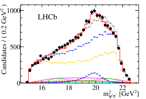
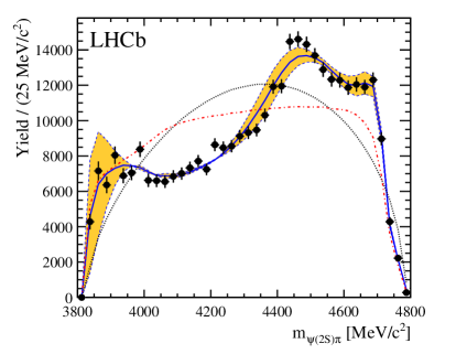
   Figure 1: Left panel: Invariant mass distributions in $\psi^{\prime}\,\pi^{-}$ channel, from Ref. [8]. The red solid (brown dashed) curve shows the fit with (without) the additional $Z(4430)$ resonance. Right panel: the Legendre moments populated by $\pi K$ waves with $J\leq 3$ are not able to describe data (from Ref. [9]). Although the agreement in the figure may look good, the significance of higher momenta is $8\sigma$.

2. Analyticity constraints for $B\to\psi^{\prime}\pi K$

   In the modern literature, there seems to be a lot of confusion regarding properties of the reaction amplitudes employed in analyses of such processes. This is often stated in the context of a potentially nonrelativistic character of certain approaches [12, 13, 14, 15, 16, 17]. As discussed in Ref. [18], rather than arising from relativistic kinematics, the differences between the various formalisms have a dynamical origin.

   We consider the scattering process $\psi^{\prime}B\to\pi K$, related to the decay we are interested in via crossing symmetry. The spinless particles $B$, $\pi$, $K$ are stable against the strong interaction, and the $\psi^{\prime}$ is narrow enough to completely factorize its decay dynamics. We use $p_{i}$, $i=1\dots 4$ to label the momenta of $\psi^{\prime}$, $B$, $\pi$, and $K$ respectively. We denote the helicity amplitude by $\mathcal{A}_{\lambda}(s,t)$, $\lambda$ being the helicity of $\psi^{\prime}$. The amplitude depends on the standard Mandelstam variables $s=(p_{3}+p_{4})^{2}$, $t=(p_{1}-p_{3})^{2}$, and $u=(p_{1}-p_{4})^{2}$ with $s+t+u=\sum_{i}m_{i}^{2}$.

   We discuss the parity violating amplitude. We call $p$ ($q$) to the magnitude of the incoming (outgoing) three momentum in the $s$-channel center of mass, and $\theta_{s}$ the scattering angle. The quantities depend on the Mandelstam invariants through

   $$z_{s} \equiv\cos\theta_{s}=\frac{s(t-u)+(m_{1}^{2}-m_{2}^{2})(m_{3}^{2}-m_{4}^{2})}{\lambda^{1/2}_{12}\lambda_{34}^{1/2}}, p =\frac{\lambda^{1/2}_{12}}{2\sqrt{s}}, q =\frac{\lambda^{1/2}_{34}}{2\sqrt{s}},$$ (1)

   with $\lambda_{ik}=\left(s-(m_{i}+m_{k})^{2}\right)\left(s-(m_{i}-m_{k})^{2}\right)$. We assume the isobar model, and incorporate the $\pi K$ resonances up to spin $J_{\text{max}}$ via

   $$A_{\lambda}(s,t,u)=\frac{1}{4\pi}\sum_{j=|\lambda|}^{J_{\text{max}}}(2j+1)A_{\lambda}^{j}(s)\,d_{\lambda 0}^{j}(z_{s}),$$ (2)

   where $A^{j}_{\lambda}(s)$ are the helicity partial wave amplitudes in the $s$-channel. In Eq. (2) the entire $t$ dependence enters though the $d$ functions. The $d$ functions have singularities in $z_{s}$ which lead to kinematical singularities in $t$ of the helicity amplitudes $A_{\lambda}$. An extensive discussion and the full characterization of the kinematical singularities can be found in Refs. [19, 20, 21, 22, 23, 24]. We recall that $d_{\lambda 0}^{j}(z_{s})=\hat{d}_{\lambda 0}^{j}(z_{s})\xi_{\lambda 0}(z_{s})$, where $\xi_{\lambda 0}(z_{s})=\left(\sqrt{1-z_{s}^{2}}\right)^{|\lambda|}$ is the so-called half angle factor that contains all the kinematical singularities in $t$. The reduced rotational function $\hat{d}_{\lambda 0}^{j}(z_{s})$ is a polynomial in $s$ and $t$ of order $j-|\lambda|$ divided by the factor $\lambda_{12}^{(j-|\lambda|)/2}\lambda_{34}^{(j-|\lambda|)/2}$. The helicity partial waves $A_{\lambda}^{j}(s)$ have singularities in $s$. These have both dynamical and kinematical origin. The former arise, for example, from $s$-channel resonances. The kinematical singularities, just like the $t$-dependent kinematical singularities, arise because of external particle spin. We explicitly isolate the kinematic factors in $s$, and denote the kinematical singularity-free helicity partial wave amplitudes by $\hat{A}_{\lambda}^{j}(s)$,

   $$A_{0}^{j}(s) =K_{00}\,\left(pq\right)^{j}\,\hat{A}_{0}^{j}(s),$$ (3a)

   $$A_{\pm}^{j}(s) =K_{\pm 0}\,\left(pq\right)^{j-1}\,\hat{A}_{\pm}^{j}(s),$$ (3b)

   with $K_{00}=2m_{1}/\lambda_{12}^{1/2}$, and $K_{\pm 0}=\lambda_{34}^{1/2}/2\sqrt{s}$. The $j=0$ amplitude is exceptional, $A_{0}^{0}(s)=\hat{A}_{0}^{0}(s)/K_{00}$. The $\hat{A}_{\lambda}^{j}(s)$ are left as the dynamical functions we are after, usually parameterized in terms of a sum of Breit-Wigner amplitudes with Blatt-Weisskopf barrier factors. We now seek a representation of $A_{\lambda}(s,t)$ in terms of the scalar functions,

   $$A_{\lambda}(s,t)=\epsilon_{\mu}(\lambda,p_{1})\left[(p_{3}-p_{4})^{\mu}-\frac{m_{3}^{2}-m_{4}^{2}}{s}(p_{3}+p_{4})^{\mu}\right]C(s,t)+\epsilon_{\mu}(\lambda,p_{1})(p_{3}+p_{4})^{\mu}B(s,t),$$ (4)

   where the functions $B(s,t)$ and $C(s,t)$ are the kinematical singularity free scalar amplitudes. We can match Eqs. (2) and (4), and express the scalar functions as a sum over kinematical singularity free helicity partial waves.

   $$\sqrt{2}\,C(s,t) =\frac{1}{4\pi}\sum_{j>0}(2j+1)(pq)^{j-1}\hat{A}_{\pm}^{j}(s)\,\hat{d}_{10}^{j}(z_{s}),$$ (5)

   $$4\pi B(s,t) =\hat{A}_{0}^{0}(s)+\frac{4m_{1}^{2}}{\lambda_{12}}\sum_{j>0}(2j+1)(pq)^{j}$$

   $$\qquad\times\left[\hat{A}_{0}^{j}(s)\hat{d}_{00}^{j}(z_{s})+\frac{s+m_{1}^{2}-m_{2}^{2}}{\sqrt{2}m_{1}^{2}}\hat{A}_{+}^{j}(s)\,z_{s}\hat{d}_{10}^{j}(z_{s})\right].$$ (6)

   Neither $B(s,t)$ nor $C(s,t)$ can have kinematical singularities in $s$ or $t$. In Eqs. (5)-(2), $\hat{d}^{j}_{10}(z_{s})$ is regular in $t$, and the $s$ singularities at (pseudo)thresholds are canceled by the factor $(pq)^{j-1}$. For the same reason the sum in Eq. (2) has no kinematical singularities in $s$ and $t$, however the $1/\lambda_{12}$ factor in front of the sum generates two poles at $s_{\pm}=(m_{1}\pm m_{2})^{2}$, unless the expression in brackets vanishes at those points. This means that the $\hat{A}^{j}_{\lambda}(s)$ with different $\lambda$ cannot be independent functions at the (pseudo)threshold. Explicitly, using the expansion of the Wigner $d$-function for $z_{s}\to\infty$, we get

   $$\hat{A}_{0}^{j}(s)\frac{(z_{s})^{j}}{\langle j-1,0;1,0|j,0\rangle}-\frac{s+m_{1}^{2}-m_{2}^{2}}{\sqrt{2}\>m_{1}^{2}}\hat{A}_{+}^{j}(s)\,\frac{(z_{s})^{j}}{\sqrt{2}\>\langle j-1,0;1,1|j,1\rangle}.$$ (7)

   This combination has to vanish to cancel the $1/\lambda_{12}$, thus one finds (for $j>0$)

   $$\hat{A}_{+}^{j}(s) =\langle j-1,0;1,1|j,1\rangle\>g_{j}(s)+\lambda_{12}\>f_{j}(s),$$ (8a)

   $$\hat{A}_{0}^{j}(s) =\langle j-1,0;1,0|j,0\rangle\frac{s+m_{1}^{2}-m_{2}^{2}}{2m_{1}^{2}}\>g^{\prime}_{j}(s)+\lambda_{12}\>f_{j}^{\prime}(s),$$ (8b)

   where $g_{j}(s)$, $f_{j}(s)$, $g^{\prime}_{j}(s)$, and $f^{\prime}_{j}(s)$ are regular functions at $s=s_{\pm}$, and $g_{j}(s_{\pm})=g^{\prime}_{j}(s_{\pm})$. Together with Eq. (8), the expressions in Eqs. (4), (5) and (2) provide the most general parameterization of the amplitude that incorporates the minimal kinematic dependence that generates the correct kinematical singularities as required by analyticity.

   Upon restoration of the kinematic factors, the original helicity partial wave amplitudes read

   $$A_{+}^{j}(s) =p^{j-1}q^{j}\bigg{[}\langle j-1,0;1,1|j,1\rangle\>g_{j}(s)+\lambda_{12}\>f_{j}(s)\bigg{]},$$ (9a)

   $$A_{0}^{j}(s) =p^{j-1}q^{j}\bigg{[}\langle j-1,0;1,0|j,0\rangle\>\frac{s+m_{1}^{2}-m_{2}^{2}}{2m_{1}\sqrt{s}}\>g^{\prime}_{j}(s)+\frac{m_{1}}{\sqrt{s}}\lambda_{12}\>f_{j}^{\prime}(s)\bigg{]},$$ (9b)

   and $A_{0}^{0}(s)=\lambda_{12}^{1/2}/(2m_{1})\,\hat{A}_{0}^{0}(s)$, where $\hat{A}_{0}^{0}(s)$ is regular at (pseudo)threshold. A particular choice of the functions $g_{j}(s)$, $g_{j}^{\prime}(s)$, $f_{j}(s)$ and $f_{j}^{\prime}(s)$ constitutes a given hadronic model.

   We now compare the general expression for the helicity partial waves with the spin-orbit LS partial waves, $\hat{G}^{j}_{L}(s)$. These match the general form in Eq. (8) when

   $$g_{j}(s) =\textstyle{\sqrt{\frac{2j-1}{2j+1}}}\hat{G}^{j}_{j-1}(s), f_{j}(s) =\frac{1}{4s}\textstyle{\sqrt{\frac{2j+3}{2j+1}}}\langle j+1,0;1,1|j,1\rangle\>\hat{G}^{j}_{j+1}(s),$$ (10a)

   $$g^{\prime}_{j}(s) =\frac{2m_{1}\sqrt{s}}{s+m_{1}^{2}-m_{2}^{2}}\textstyle{\sqrt{\frac{2j-1}{2j+1}}}\hat{G}^{j}_{j-1}(s), f_{j}^{\prime}(s) =\frac{1}{4m_{1}\sqrt{s}}\textstyle{\sqrt{\frac{2j+3}{2j+1}}}\langle j+1,0;1,0|j,0\rangle\>\hat{G}^{j}_{j+1}(s).$$ (10b)

   The common lore is that the LS formalism is intrinsically nonrelativistic. However, the matching in Eq. (10) proves that the formalism is fully relativistic, but care should be taken when choosing a parameterization of the LS amplitude so that the expressions in Eqs. (10) are free from kinematical singularities. For example, if one takes the functions $\hat{G}^{j}_{j-1}(s)$ and $\hat{G}^{j}_{j+1}(s)$ to be proportional to Breit-Wigner functions with constant couplings, the amplitudes $g^{\prime}_{j}(s)$ and $f^{\prime}_{j}(s)$ would end up having a pole at $s=m_{2}^{2}-m^{2}_{1}$. It is clear that using Breit-Wigner parameterizations, or any other model for helicity amplitudes, i.e., the left-hand sides of Eq. (10), instead of the LS amplitudes helps prevent unwanted singularities.

   We also consider the Covariant Projection Method (CPM) approach of [12, 13, 14, 15], based on the construction of explicitly covariant expressions. We limit ourselves to the special case of an intermediate $K^{\ast}$ with $j=1$. We start with the tensor amplitude for the scattering process $\psi B\to K^{\ast}\to\pi K$,

   $$A_{\lambda}(s,t) =\epsilon_{\mu}(\lambda,p_{1})\left(-g^{\mu\nu}+\frac{P^{\mu}P^{\nu}}{s}\right)X_{\nu}(q,P)g_{S}(s)$$

   $$\qquad+\epsilon^{\rho}(\lambda,p_{1})X_{\rho\mu}(p,P)\left(-g^{\mu\nu}+\frac{P^{\mu}P^{\nu}}{s}\right)X_{\nu}(q,P)g_{D}(s),$$ (11)

   where $P$ is the $K^{\ast}$ momentum. The final P-wave orbital tensor is $X_{\nu}(q,P)=q^{\perp}_{\nu}=q_{\nu}-P_{\nu}P\cdot q/s$. The D-wave orbital tensor $X^{\rho\mu}(p,P)=3p^{\rho}_{\perp}p^{\mu}_{\perp}/2-g^{\rho\mu}_{\perp}p_{\perp}^{2}/2$, with $p_{\perp}^{\mu}=p^{\mu}-P^{\mu}\,P\cdot p/s$, and $g^{\rho\mu}_{\perp}=g^{\rho\mu}-P^{\rho}P^{\mu}/s$. Explicitly,

   $$A_{+}(s,\theta_{s})=-q\frac{\sin\theta_{s}}{\sqrt{2}}\left[g_{S}(s)+\frac{p^{2}}{2}g_{D}(s)\right],\quad A_{0}(s,\theta_{s})=q\frac{E_{1}}{m_{1}}\cos\theta_{s}\left[g_{S}(s)-p^{2}g_{D}(s)\right],$$ (12)

   and matching with Eq. (8) gives

   $$g_{1}(s) =g_{1}^{\prime}(s)=\frac{4\pi}{3}g_{S}(s), f_{1}(s) =\frac{2\pi}{3s}g_{D}(s), f_{1}^{\prime}(s) =-\frac{4\pi}{3s}\frac{s+m_{1}^{2}-m_{2}^{2}}{m_{1}^{2}}g_{D}(s).$$ (13)

   

   

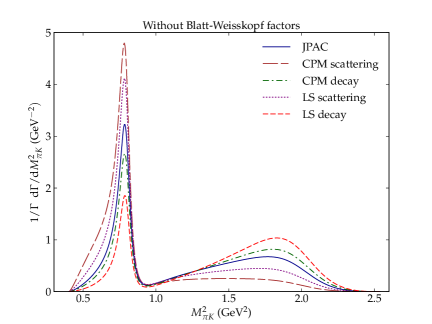
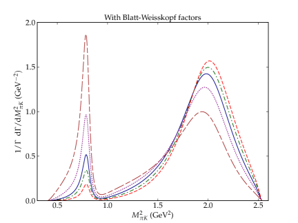
   Figure 2: Comparison of the lineshape of $K^{\ast}(892)$ and $K^{\ast}(1410)$ in the $\pi K$-invariant mass distribution, constructed with the different formalisms. In the left panel we show the result with no barrier factors. In the right panel, we include the customary Blatt-Weisskopf factors. From [18].

   The threshold conditions $g_{1}(s_{\pm})=g_{1}^{\prime}(s_{\pm})$ are satisfied, and the functions $f_{1}(s)$ and $f_{1}^{\prime}(s)$ are regular at the thresholds. Finally, we show the relation between the CPM and the LS amplitudes:

   $$\frac{3}{4\pi}G_{0}^{1}(s) =g_{S}(s)\>q\>\sqrt{\frac{1}{3}}\left(\frac{E_{1}}{m_{1}}+2\right)-g_{D}(s)\>q\>p^{2}\>\sqrt{\frac{1}{3}}\left(\frac{E_{1}}{m_{1}}-1\right),$$ (14a)

   $$\frac{3}{4\pi}G_{2}^{1}(s) =g_{D}(s)\>q\>p^{2}\>\sqrt{\frac{1}{6}}\left(2\frac{E_{1}}{m_{1}}+1\right)-g_{S}(s)\>q\>\sqrt{\frac{2}{3}}\left(\frac{E_{1}}{m_{1}}-1\right).$$ (14b)

   Although the $g_{S}(s)$ and $g_{D}(s)$ of the CPM formalism, see Eq. (11), are typically interpreted as the $S$ and $D$ partial wave amplitudes, we see that this is the case only at (pseudo)threshold $s=s_{\pm}$, where the factor $E_{1}/m_{1}-1$ vanishes. An extensive discussion about the same calculation performed in the decay kinematics, which turns out into an explicit violation of crossing symmetry, can be found in [18].

   To explore the differences between the various approaches, we consider the example of two intermediate vectors in the $\pi K$ channel: the $K^{\ast}(892)$, with mass and width $M_{K^{\ast}}=892$ MeV, $\Gamma_{K^{\ast}}=50$ MeV, and the $K^{\ast}(1410)$, with $M_{K^{\ast}}=1414$ MeV, $\Gamma_{K^{\ast}}=232$ MeV.

   In Fig. 2, we show the results for the differential decay width in five different scenarios. We consider the CPM formalism (for the scattering and decay kinematics, respectively), setting $g_{S}(s)=0$ and $g_{D}(s)=T_{K^{\ast}}(s)$, with $T_{K^{\ast}}(s)$ being the sum of Breit-Wigners for the two resonances. For the LS formalism, we choose the couplings to be $\hat{G}_{0}^{1}(s)=0$, $\hat{G}_{2}^{1}(s)=T_{K^{\ast}}(s)$. The LS amplitude in the decay kinematics differs from the one in the scattering kinematics because of the breakup momentum of $B\to\psi K^{\ast}$, calculated in the $B$ rest frame or in the $K^{\ast}$ rest frame, respectively. In Ref. [18] we also propose an alternative model. We see in Fig. 2 that the $K\pi$ invariant mass squared distribution is significantly distorted in all models. This is important to extract the physical couplings, and may enhance the high mass contributions of the higher spin $K^{\ast}$, thus affecting the extraction of the properties of the $Z(4430)$.

3. Conclusions

   

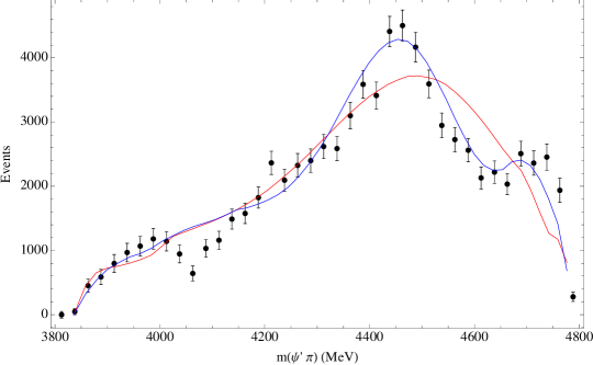
   Figure 3: Fit to the $\psi^{\prime}\pi$ invariant mass, in the $1\leavevmode\nobreak\ GeV\leq m(\pi K)\leq 1.39\leavevmode\nobreak\ GeV$ slice, where the signal of the $Z(4430)$ is more prominent. The red curve includes the $K^{\ast}$ resonances with $J\leq 3$, whereas the blue curve includes the tails of the $K_{4}^{\ast}(2045)$ and the $K_{5}^{\ast}(2380)$. Data from [9].

   The rich structure of the $\pi K$ system affects the extraction of several exotic candidates, as the $Z(4200)$ in $B\to J/\psi\pi K$ [25], the $Z(4050)$ and $Z(4250)$ in $B\to\chi_{c1}\,\pi K$ [26, 27], and in particular the $Z(4430)$ in $B\to\psi^{\prime}\,\pi K$ we have discussed here [4, 5, 6, 7, 8, 9]. As we show in a temptative fit in Fig. 3, the inclusion of higher spin $K^{\ast}$ resonances can improve the description of the $\psi^{\prime}\pi$ invariant mass, even without adding an exotic state. Although this may not be enough to challenge the existence of the $Z(4430)$, this can dramatically affect the estimate of the resonance parameters and of its quantum numbers. This also calls for more refined analysis, which take into account unitarity in the isobar model [28, 29, 30, 31, 32, 33, 34, 35], or include the effect of higher spin resonances [36].

4. Acknowledgments

   I wish to thank Igor Strakovsky for his kind invitation to this workshop, and Tomasz Skwarnicki for the fruitful collaboration. My participation to the conference was supported by the U.S. Department of Energy, Office of Science, Office of Nuclear Physics under contract DE–AC05–06OR23177.

3.18 Three Particle Dynamics on the Lattice

Akaki Rusetsky

Helmoltz-Institut für Strahlen- und Kernphysik

Universität Bonn &

Bethe Center for Theoretical Physics

Universität Bonn

D-53115 Bonn, Germany

1. Introduction

   The Lüscher approach [4] has become a standard tool for the analysis of lattice data in the two-body scattering sector. It has been further generalized to study the scattering of particles with arbitrary spin, the scattering in the moving frames, as well as the scattering in coupled two-body channels. Moreover, in their seminal paper [5], Lellouch and Lüscher have discussed the application of the finite-volume formalism to the calculation of the two-body decay matrix elements. This approach has been also generalized to include multiple decay channels and applied to study of various formfactors in the timelike region and matrix elements with resonances (in the latter case, the analytic continuation in the complex plane to the resonance pole has to be considered) [6, 7, 8, 9].

   The formulation of the finite-volume approach for the three-body problem (in analogy with the Lüscher approach) has however proven to be a challenging task. Despite the significant effort during the last few years [1, 2, 3, 10, 11, 12, 13, 14, 15, 16, 17, 18, 19, 20], the progress has been rather slow. Recently, the tree-body quantization condition, which is a counterpart of the Lüscher equation in the two-body case, has been derived in different settings [12, 11, 1, 2, 17] (it has been shown [3] that all these different settings are essentially equivalent to each other, so in practice all boils down to the choice of merely the most convenient one). On the basis of the quantization condition, the finite-volume energy levels have been calculated in some simple cases. Such studies are extremely interesting because, at this stage, one does not yet have enough insight in the problem and lacks the intuition to predict the volume dependence of the three-body spectrum, which would emerge in lattice simulations. Moreover, such studies may facilitate the interpretation of this volume dependence in terms of the observable characteristics of the three-particle systems in a finite volume, in analogy with the two-particle case where, e.g., the avoided level crossing in the spectrum is often related to a nearby narrow resonance.

   The study of the three-particle (and, in general, many-particle) systems on the lattice is interesting at least from two different perspectives. First, we would refer to the potential applications in study of the nuclear physics problems in lattice QCD. Second, it would be interesting to study the systems, whose decay into the final states with three and more particles cannot be neglected. In the meson sector, the simplest example could be the decay $K\to 3\pi$ (a counterpart of the process $K\to 2\pi$, which was considered in the original paper by Lellouch and Lüscher [5]), but physically more interesting processes like the decays of $a_{1}(1260)$ or $a_{1}(1420)$ as well. In the baryon sector, the most obvious candidate is the Roper resonance. In order to obtain an analog of the Lellouch-Lüscher formula for such systems, however, one has first to understand the final-state interactions in a finite volume, and it is where the study of the solutions of the three-body quantization condition might help.

   In my talk, I shall briefly cover the formalism of Refs. [1, 2], which is based on the use of the effective field theory in a finite volume, and will further discuss the solution of these equations, which includes the projection of the quantization condition onto the different irreducible representations (irreps) of the octahedral group [3]. It will be shown that these solutions allow for a nice interpretation in terms of the three-particle bound states, as well as three-particle and particle-dimer scattering states.

2. The Formalism

   In Refs. [1, 2], the three-particle quantization condition was obtained by using effective field theory approach in a finite volume. Moreover, it has been shown that it is very convenient to use the so-called particle-dimer picture. It should be stressed that this approach is not an approximation, but an equivalent description of the three-particle interactions. This is most easily seen in the path integral formalism, where the introduction of a dimer amounts to using an additional dummy integration variable, without changing the value of the path integral. Moreover, using the particle-dimer picture does not necessarily imply the existence of a shallow bound state or a narrow resonance in the two-body sector.

   Below we consider the case of three identical spinless bosons with the S-wave pair interactions and use, for simplicity, the non-relativistic kinematics. In order to derive the quantization condition, we consider the finite-volume Bethe-Salpeter equation for the particle-dimer amplitude ${\cal M}_{L}$

   $${\cal M}_{L}({\bf p},{\bf q};E)=Z({\bf p},{\bf q};E)+\frac{1}{L^{3}}\,\sum_{\bf k}^{\Lambda}Z({\bf p},{\bf k};E)\,\tau_{L}({\bf k};E)\,{\cal M}_{L}({\bf k},{\bf q};E)\,.$$ (1)

   Here, ${\bf p}$ and q are three-momenta of the incoming and outgoing spectators and $E$ is the total energy of three particles. All momenta are discretized, e.g., ${\bf p}=2\pi{\bf n}/L,\leavevmode\nobreak\ {\bf n}\in\mathbb{Z}^{3}$ and, similarly, for other momenta. Further, $L$ is the spatial size of the cubic box and $\Lambda$ denotes the ultraviolet cutoff. The quantity $\tau_{L}$ corresponds to the two-body scattering amplitude (the dimer propagator, in the particle-dimer language), and is given by

   $$8\pi\tau_{L}^{-1}({\bf k};E) = k^{\ast}\cot\delta(k^{\ast})+S({\bf k},(k^{\ast})^{2})\,,$$

   $$S({\bf k},(k^{\ast})^{2}) = -\frac{4\pi}{L^{3}}\sum_{\bf l}\frac{1}{{\bf k}^{2}+{\bf k}{\bf l}+{\bf l}^{2}-mE}\,,$$ (2)

   where $k^{\ast}$ is the magnitude of the relative momentum of the pair in the rest frame,

   $$k^{\ast}=\sqrt{\frac{3}{4}\,{\bf k}^{2}-mE}\,.$$ (3)

   In Eq. (2), unlike Eq. (1), the momentum sum is implicitly regularized by using dimensional regularization and $\delta(k^{\ast})$ is the S-wave phase shift in the two-particle subsystem. The effective range expansion for this quantity reads

   $$k^{\ast}\cot\delta(k^{\ast})=-\frac{1}{a}+\frac{1}{2}\,r(k^{\ast})^{2}+O((k^{\ast})^{4})\,,$$ (4)

   where $a,r$ are the two-body scattering length and the effective range, respectively. In the numerical calculations, for illustrative purpose, we shall use a simplified model, assuming that the effective range $r$ and higher-order shape parameters are all equal to zero, corresponding to the leading order of the effective field theory for short range-interactions. The equation (1) is valid, however, beyond this approximation.

   Finally, the quantity $Z$ denotes the kernel of the Bethe-Salpeter equation. It contains the one-particle exchange diagram, as well as the local term, corresponding to the particle-dimer interaction (three-particle force). In general, the latter consists of a string of monomials in the 3-momenta ${\bf p}$ and ${\bf q}$. In the numerical calculations, we shall again restrict ourselves to the model, where only the non-derivative coupling, which is described by a single constant $H_{0}(\Lambda)$, is non-vanishing. The kernel then takes the form

   $$Z({\bf p},{\bf q};E)=\frac{1}{-mE+{\bf p}^{2}+{\bf q}^{2}+{\bf p}{\bf q}}+\frac{H_{0}(\Lambda)}{\Lambda^{2}}\,.$$ (5)

   The dependence of $H_{0}(\Lambda)$ on the cutoff is such that the infinite-volume scattering amplitude is cutoff-independent. In a finite volume, this ensures the cutoff-independence of the spectrum.

   At the next step, the three-particle Green function can be expressed in terms of the particle-dimer scattering amplitude ${\cal M}_{L}$ by using the LSZ formalism, and hence the poles of the latter can be mapped onto the finite-volume energy spectrum of the three particle system. It can be shown [3] that the poles arise at the energies, where the determinant of the linear equation (1) vanishes. This finally gives the quantization condition we are looking for

   $$\det(\tau_{L}^{-1}-Z)=0\,.$$ (6)

   The l.h.s. of the above equation defines a function of the total energy $E$, which, for a fixed $\Lambda$ and $L$, depends both on the two-body input (the scattering phase $\delta$ both above and below the two-body threshold) as well as the three-body input (the non-derivative coupling $H_{0}(\Lambda)$, higher-order couplings). The former input can be independently determined from the simulations in the two-particle sector and extrapolation below threshold. Hence, measuring the three-particle energy levels, one will be able to fit the parameters of the three-body force. Finally, using the same equations in the infinite volume with the parameters, determined on the lattice, one is able to predict the physical observables in the infinite volume.

3. The Projection of the Quantization Condition

   The three-body quantization condition, Eq. (6), determines the entire finite-volume spectrum of the system. However, the eigenvalue problem in a cubic box has the octahedral symmetry, which is a remnant of the rotational symmetry in the infinite volume. This means that all energy levels can be assigned to one of the ten irreps $A_{1}^{\pm},A_{2}^{\pm},E^{\pm},T_{1}^{\pm},T_{2}^{\pm}$ of the octahedral group ${\cal G}$ and the spectrum in each irrep can be measured separately with a proper choice of the source/sink operators. It is possible to use this symmetry and to project the quantization condition onto the different irreps – the obtained equations will determine the energy spectrum in each irrep separately [3].

   In order to do this, we shall act in a close analogy with the partial-wave expansion in the infinite volume. A substitute for radial integration will be the sum over shells, defined as sets of momenta with equal magnitude, which can be obtained from any vector (referred hereafter as the reference vector), belonging to the same shell, by applying all transformations of the octahedral group. Note that the vectors with the same magnitude, which are not connected by a group transformation belong, by definition, to different shells. Furthermore, the integration over the solid angle in the infinite volume is replaced by the sum over all $G=48$ elements of the octahedral group.

   On the cubic lattice, the analog of the partial-wave expansion is given by

   $$f({\bf p})=f(g{\bf p}_{0})=\sum_{\Gamma}\sum_{\rho\sigma}T^{\Gamma}_{\sigma\rho}(g)f^{\Gamma}_{\rho\sigma}(s)\,,\quad\quad\Gamma=A_{1}^{\pm},A_{2}^{\pm},E^{\pm},T_{1}^{\pm},T_{2}^{\pm}\,,$$ (7)

   where $T^{\Gamma}_{\sigma\rho}(g)$ are the matrices of the irreducible representations, ${\bf p}_{0}$ denotes the reference momentum, and $s$ is the shell to which both ${\bf p}$ and ${\bf p}_{0}$ belong. Nothing depends on the choice of ${\bf p}_{0}$.

   Using the orthogonality of the matrices of the irreducible representations, it is possible to project out the quantity $f^{\Gamma}_{\rho\sigma}(s)$:

   $$\sum_{g\in{\cal G}}(T^{\Gamma}_{\lambda\delta}(g))^{\ast}f(g{\bf p}_{0})=\frac{G}{s_{\Gamma}}\,f^{\Gamma}_{\delta\lambda}(s)\,,$$ (8)

   where $s_{\Gamma}$ is the dimension of the irrep $\Gamma$, and the indices $\lambda,\delta,\ldots$ run from 1 to $s_{\Gamma}$.

   Next, we note that both the kernel of the Bethe-Salpeter equation and the dimer propagator are invariant with respect to the group ${\cal G}$:

   $$Z(g{\bf p},g{\bf q};E)=Z({\bf p},{\bf q};E)\,,\quad\quad\tau_{L}(g{\bf k};E)=\tau_{L}({\bf k};E)\,,\quad\quad\mbox{for all}\leavevmode\nobreak\ g\in{\cal G}\,.$$ (9)

   Using this property, it can be shown that the projection of the quantization condition onto the irrep $\Gamma$ takes the form

   $$\det\biggl{(}\tau_{L}(s)^{-1}\delta_{rs}\delta_{\sigma\rho}-\frac{\vartheta(s)}{GL^{3}}\,Z^{\Gamma}_{\sigma\rho}(r,s)\biggr{)}=0\,,$$ (10)

   where $\vartheta(s)$ is the multiplicity of the shell $s$ (the number of independent vectors in this shell), and

   $$Z^{\Gamma}_{\lambda\rho}(r,s)=\sum_{g\in{\cal G}}(T^{\Gamma}_{\rho\lambda}(g))^{\ast}Z(g{\bf p}_{0},{\bf k}_{0})\,.$$ (11)

   Here, the reference vectors ${\bf p}_{0}$ and ${\bf k}_{0}$ belong to the shells $r$ and $s$, respectively. In the next section, we shall solve this equation and obtain the spectrum of both the bound and scattering states.

4. The Energy Spectrum

   1. The Choice of the Model

      In order to gain insight into the volume-dependence of the three-particle spectrum, we shall solve the equation (10) in the irrep $\Gamma=A_{1}^{+}$ in a simple model, described in section 2. The parameters of the model are fixed as follows. First, we take $m=a=1$. This means that there exists a bound dimer with the binding energy $B_{2}=\frac{1}{ma^{2}}=1$. Further, we fix the ultraviolet cutoff $\Lambda=225$ – large enough so that all cutoff artifacts can be safely neglected. The last remaining parameter $H_{0}(\Lambda)$ is fixed from the requirement that there exists a three-body bound state with the binding energy $B_{3}=10$. This gives $H_{0}(\Lambda)=0.192$. Of course, for a different choice of $\Lambda$, one may adjust $H_{0}(\Lambda)$, so that all low-energy spectrum remains the same.

   2. Bound States

      Except of the already mentioned deeply bound three-body state with $B_{3}=10$, the model contains an extremely shallow bound state with $B_{3}=1.016$ – just below the particle-dimer threshold. Since the characteristic size of such system is much larger than that of the dimer, it is conceivable that it should behave like a two-body bound state of a particle and a dimer. For the deep bound state, two-particle and three-particle bound-state scales are comparable in magnitude and hence one might expect a behavior that interpolates between the extreme cases of a three-particle shallow bound state and a particle-dimer bound state.

      It is quite intriguing that the study of the finite-volume spectrum allows one to make a choice among the above alternatives. It is, in particular, well known that the Lüscher equation leads to the finite-volume correction $\propto\exp(-\Delta L)/L$ to the infinite-volume binding energy (here, $\Delta$ is some mass scale determined by the kinematics). The functional dependence of the three-body shallow bound state is different,
      $\propto\exp(-\Delta L)/L^{3/2}$, see, e.g., Refs. [18]. So, the volume dependence of the binding energy contains information about the nature of the three-body bound states.

      Among the solutions of the quantization condition (10) one can readily identify the levels that tend to the infinite-volume binding energies. It is seen that the volume-dependence of the shallow bound state can be approximated by the function
      $\propto\exp(-\Delta L)/L$ very well. For the deeper state, the situation is different and one needs a linear combination of the above two functions to get a decent fit. All this of course perfectly matches our expectations. More details can be found in Ref. [3].

   3. Scattering States

      There are two types of the non-interacting energy levels, corresponding to the different asymptotic states in the three-body problem. In particular, we have the particle-dimer scattering states with different back-to-back momenta. The threshold for such states is given by the dimer binding energy and lies at $E_{th}=-1$. In addition to this, we have free 3-particle states with the threshold $E_{th}^{0}=0$. Of course, in the interacting theory, which we are considering, the energy levels are displaced from their “free” values, but the displacement is relatively small almost everywhere. For this reason, one can identify the levels of the interacting theory with the different free levels.

      

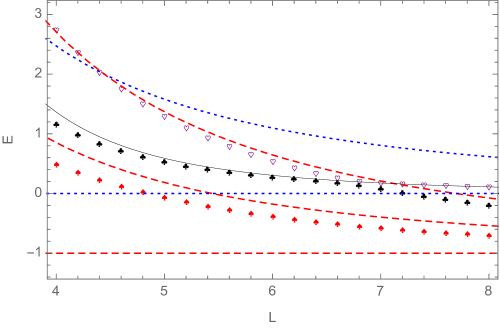
      Figure 1: The three lowest-lying states above threshold. The result obtained using Eq. (12) is given by the black solid curve. The red dashed curve shows the free particle-dimer states with back-to-back momenta $(0,0,0)$, $(0,0,1)$ and $(1,1,0)$, whereas the blue dotted lines denote the free three-particle states (the lowest level at $E=0$ corresponds to the threshold, where all three particles are at rest).

      In Fig. 1, the volume-dependence of the three lowest scattering states, obtained from the solution of Eq. (10), is shown. For comparison, in the same figure, we plot the free particle-dimer and three-particle energy levels.

      Last but not least, we plot the displaced ground-state energy of three particles which, up to and including order $L^{-5}$, is given by the formula (see, e.g., Refs. [21, 13])

      $$E=\frac{12\pi a}{L^{3}}-\frac{12a^{2}}{L^{4}}\,{\cal I}+\frac{12a^{3}}{\pi L^{5}}({\cal I}^{2}+{\cal J})+O(L^{-6})\,,$$ (12)

      where ${\cal I}\simeq-8.914$ and ${\cal J}\simeq 16.532$ are numerical constants. It is seen that, at this accuracy, the energy shift from the unperturbed value $E=0$ contains only the single parameter $a$ which is fixed from the beginning. Thus, Eq. (12) constitutes a prediction that allows to identify the three-particle ground state.

      The interpretation of the levels, shown in Fig. 1 is crystal clear. The lowest level is a displaced particle-dimer ground state. Its relatively large displacement is caused by the existence of a very shallow three-body bound state, which pushes all other particle-dimer levels up. At small values of $L$, the next level is the displaced three-body ground state. Around $L\simeq 7$, free particle-dimer and three-particle levels cross each other. This fact leads to the avoided level crossing in the interacting spectrum, the second level goes down to the particle-dimer threshold and the third level becomes the displaced ground-state three-particle level. This pattern repeats itself each time, when we have a crossing of two levels corresponding to the different asymptotic states. For more details, see Ref. [3].

5. Conclusions

   • We use the effective field theory approach in a finite volume to obtain the three-particle quantization condition. The fit of the solutions of this equation to the three-particle finite-volume spectrum determines the particle-dimer coupling constant(s), which can be further used in the Bethe-Salpeter equation to reconstruct the infinite-volume scattering amplitudes in the three-particle sector. This is the essence of the approach proposed in Refs. [1, 2].

   • Using the octahedral symmetry of the problem in a cubic box, the quantization condition was projected onto the different irreps of this symmetry group.

   • The equation was numerically solved in the $A_{1}^{+}$ irrep, both for the bound states and scattering states. It was shown that a nice interpretation of the energy levels is possible in terms of the different asymptotic states of the three-particle system. In particular, it was shown that the avoided level crossing occurs at those values of $L$, when the free levels, corresponding to these states, have the same energy.

6. Acknowledgments

   The author acknowledges the support from the CRC 110 “Symmetries and the Emergence of Structure in QCD” (DFG grant no. TRR 110 and NSFC grant No. 11621131001). This research was also supported in part by Volkswagenstiftung under contract no. 93562 and by Shota Rustaveli National Science Foundation (SRNSF), grant No. DI–2016–26.

3.19 S-matrix Approach to Hadron Gas: a Brief Review

Pok Man Lo

Institute of Theoretical Physics

University of Wroclaw

PL-50204 Wrocław, Poland &

Extreme Matter Institute (EMMI), GSI

D-64291 Darmstadt, Germany

1. Introduction

   The S-matrix formulation of statistical mechanics by Dashen, Ma, and Bernstein [1] expresses the grand canonical potential in terms of the scattering matrix elements. When applied to describe the system of interacting hadrons [2], the logarithm of the partition function can be written as a sum of two pieces :

   $$\ln Z =\ln Z_{0}+\Delta\ln Z,$$ (1)

   where

   $$\ln Z_{0} =V\times\sum_{i\in{\rm gs}}d_{i}\int\frac{d^{3}k}{(2\pi)^{3}}\,e^{-\beta\sqrt{k^{2}+m_{i}^{2}}}$$ (2)

   is the grand potential for an uncorrelated gas of particles that do not decay under the strong interaction (i.e., ground-state particles), such as pions, kaons, and nucleons. The interacting part of the grand potential, $\Delta\ln Z$, can be written in the form

   $$\Delta\ln Z =V\times\int d\sqrt{s}\,\,\frac{d^{3}P}{(2\pi)^{3}}\,e^{-\beta\sqrt{P^{2}+s}}\,\rho_{\rm eff}(\sqrt{s}),$$ (3)

   where $\sqrt{s}$ is the invariant mass of the relevant scattering system. The quantity $\rho_{\rm eff}(\sqrt{s})$ can be understood as an effective level density due to the interaction. A key step of the S-matrix approach to study thermodynamics is to identify such effective level density, in the low density limit where only binary collisions are important, with

   $$\rho_{\rm eff}(\sqrt{s})\rightarrow\rho_{\rm smat}(\sqrt{s})=\sum_{\rm int}d_{IJ}\times\frac{d}{d\sqrt{s}}\,\left(\frac{1}{\pi}\,\delta_{IJ}(\sqrt{s})\right).$$ (4)

   Here the sum is over all interaction channels, $d_{g}$ is the relevant degeneracy factor, and $\delta_{IJ}(\sqrt{s})$ is the scattering phase shift. Note that the standard Hadron Resonance Gas (HRG) model [3] can also be expressed in this form, with the replacement

   $$\rho_{\rm eff}(\sqrt{s})\rightarrow\rho_{\rm HRG}(\sqrt{s})=\sum_{\rm res}d_{IJ}\times\frac{d}{d\sqrt{s}}\,\left(\theta(\sqrt{s}-m_{\rm res})\right),$$ (5)

   where the sum is now over all resonances, treated as point-like particles.

   

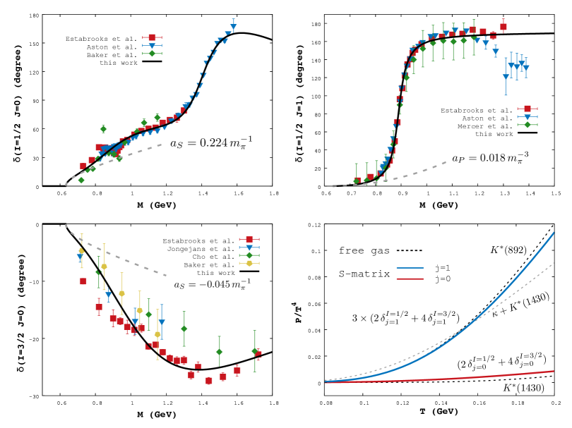
   Figure 1: $\pi K$ scattering phase shifts for the S-wave ($I=1/2,3/2$) and the P-wave ($I=1/2$), with their contributions to thermodynamic pressure.

   

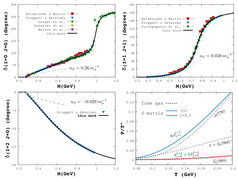
   Figure 2: $\pi\pi$ scattering phase shifts for $I=0,1,2$ and their contributions to thermodynamic pressure.

   When used in conjunction with the empirical phase shifts from scattering experiments, the S-matrix approach offers a model independent way to consistently incorporate both the attractive and repulsive forces between hadrons for the study of thermodynamics. Indeed, a very detailed picture of hadronic interactions has emerged from the impressive volume of experimental data [4], carefully analyzed by theory such as chiral perturbation theory [7, 8],lattice QCD [9], effective hadron models [10] and the classic potential models [11, 12]. Consequently we acquire very precise information on particle spectra, production mechanisms and decay properties of typical hadrons and even the exotics [13]. The method presented here is ideal for tapping into these resources in the field of hadron physics for the study of heavy ion collisions [14] and thermal properties of hadronic medium.

   In the following, we employ the approach to study some simple hadronic systems.

2. Thermal System of Pions and Kaons

   In Figs. 1 and 2, we present results for the interaction contribution to the thermodynamic pressure, computed within the S-matrix approach for $\pi K$ and $\pi\pi$ scatterings respectively. Also shown are the corresponding results from the HRG model.

   The key input here is the scattering phase shifts. Extensive experimental [15, 16, 17, 18, 19, 20, 21] and theoretical [22, 23, 24, 25] efforts are devoted to study these quantities. An efficient way to compute the effective level density in Eq. (4) is to perform a phenomenological fit to the phase shift data [22, 26]. This offers some insights into the relative importance of resonant and non-resonant contributions in an interaction channel. Nevertheless, more fundamental approaches such as chiral perturbation theory [23] and LQCD [24, 25] are in better position to implement known theoretical constraints and predict phase shifts for channels that are not yet measured.

   Let us now discuss several key features of the results in Figs. 1 and 2.

   1. S-wave Channel

      In the $I=1/2$ ($I=0$) channel of $\pi K$ ($\pi\pi$) scattering we observe a slowly rising phase shift in the low-energy region. This portion of the phase shift can reflect the physical properties of the unconfirmed $\kappa$- (confirmed $\sigma$-) meson. In particular, the phase shift does not reach $180^{\circ}$ before $K^{\ast}(1430)$ ($f_{0}(980)$) emerges. In the same energy range we also observe a major cancellation effect from the $I=3/2$ ($I=2$) channel after the multiplication of an appropriate degeneracy factor. The two effects combined severely suppress the overall pressure from these channels, down to the value of a free gas of $K^{\ast}(1430)$ ($f_{0}(980)$). This underpins the proposed prescription that $\kappa$- ($\sigma$-) meson should not be included in the HRG particle sum [26, 27].

   2. P-wave Channel

      For the $\pi K$ system, the S-matrix approach yields a similar result on the thermodynamic pressure as the HRG model. The latter is based on a point-like treatment $K^{\ast}(892)$. On the other hand, the approach gives an enhanced effect from the two-body scattering beyond the free gas result for the $\pi\pi$ system.

      

      

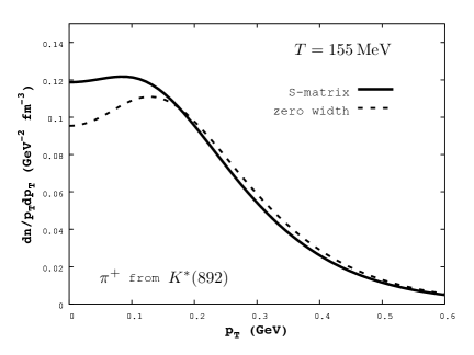
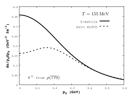
      Figure 3: The rapidity-integrated $p_{T}$ spectra of pions originated from the decay of $K^{\ast}(892)$ and $\rho(770)$ resonances ( static source, $T=155\,$ MeV ). The low-$p_{T}$ enhancement in the S-matrix treatment is clearly visible in both cases. For details see Refs. [28, 29, 31].

      It may appear that the point-particle treatment of the $K^{\ast}(892)$ resonance is a good approximation. However, this conclusion depends strongly on the observable of interest. For example, when the transverse momentum ($p_{T}$) distribution of the pions originating from a resonance decay is studied [28, 29], differences between the two approaches become appreciable. This is shown in Fig. 3. The enhancement in the S-matrix approach at the low-momentum region of the spectra originates from a non-resonant threshold effect described in Ref. [30, 28, 29, 31], which is commonly neglected in the standard HRG-based thermal models. This effect may help to account for the excess of soft pions ($p_{T}\leq 0.3$ GeV) observed in recent measurements of the LHC [32] over the predictions by conventional fluid-dynamical calculations [28].

3. Baryon Sector

   The S-matrix approach has also been applied to study the pion-nucleon system [33]. Using the empirical phase shifts from the SAID PWA database [34], it is demonstrated that the natural implementation of the repulsive forces and the consistent treatment of broad resonances can improve our understanding of fluctuation observables computed in lattice QCD, such as the baryon electric charge correlation.

   Lattice study of thermal QCD also indicates a larger interaction strength in the strange-baryon channel than that predicted by the HRG model using only the list of confirmed resonances [35]. A simple extension of the HRG model [36], which uses the lattice results to guide the incorporation of some extra hyperon states, suggests that the “missing” states required is roughly consistent with the trend of the observed but unconfirmed resonances (1 and 2 stars) in the PDG. The corresponding S-matrix based analysis is currently pursued. It is clear that a detailed experimental knowledge of the hyperon spectrum is critical for this task.

4. Summary

   The S-matrix approach offers a consistent way to incorporate attractive and repulsive forces between hadrons. Using the input of empirical phase shifts from hadron scattering experiments, the important physics of resonance widths and the contribution from purely repulsive channels are naturally included. Further research in extending the scheme [31] to include inelastic effects and three-body scatterings [37, 38, 39] has begun.

   The proposed new $K_{L}$-beam facility can potentially strengthen our understanding of the hadron spectroscopy, such as the investigation of the “missing" hyperon states. This is crucial for a reliable thermal description of the hadronic medium within the S-matrix approach. We expect interesting results when applying the approach to explore various phenomena of heavy ion collisions.

5. Acknowledgments

   I would like to thank Igor I. Strakovsky for the invitation to the Workshop. I am also grateful to Ted Barnes, Michael Döring, Jose R. Pelaez and James Ritman for the encouraging remarks and the fruitful discussion. This research benefits greatly from the discussion with Hans Feldmeier in GSI. I would also like to thank Bengt Friman, Krzysztof Redlich, and Chihiro Sasaki for the productive collaboration. Support from the Extreme Matter Institute EMMI at the GSI is gratefully acknowledged. This work was partially supported by the Polish National Science Center (NCN), under Maestro grant DEC–2013/10/A/ST2/00106.

3.20 Measurement of Hadronic Cross Sections with the BaBar Detector

Alessandra Filippi

I.N.F.N. Sezione di Torino

10125 Torino, Italy

1. Introduction

   The BaBar experiment [1] at the SLAC National Accelerator Laboratory has performed, over the last decade, a complete set of measurements of $e^{+}e^{-}$ annihilation cross sections of exclusive hadronic channels at low energies, exploiting the Initial State Radiation (ISR) technique. The main purpose of this study is to provide the most precise and complete input for the calculation of the muon anomalous magnetic moment $a_{\mu}=(g_{\mu}-2)/2$ and the running electromagnetic constant $\alpha_{EW}$. However, also several important and useful indications on the composition of the light and charmed meson spectrum could be obtained as by-products, by the inspection of the trends of the cross sections and the composition of the intermediate states of the studied reactions, as well as their decay branching fractions.

   The knowledge of the total hadronic cross section is fundamental for the determination of the hadronic vacuum polarization contribution, at leading order, to $a_{\mu}$ [2]. It is well known that a discrepancy at the level of 3.5$\sigma$ exists between the value of the muon anomolous magnetic moment expected from the Standard Model and what is experimentally observed, and the hadronic term of the sum adding up to $a_{\mu}$ is the one that bears the largest uncertainty. The dominant contribution to this term is played by the hadronic cross sections below 2 GeV, that until BaBar were measured mainly inclusively. Only recently measurements of exclusive channels could be performed accurately enough. The goal of BaBar, almost completely accomplished, was to provide measurements for all the exclusive channels below 2 GeV, comparing them with previous inclusive measurements and pQCD predictions.

   In the following a description of the measurements performed for all channels containing kaons in final states composed by a total of three or four particles will be described.

2. The Initial State Radiation (ISR) Technique and Kaon Detection with BaBar

   BaBar operated at the PEP-II machine at SLAC and had been taking data for about 10 years, up to 2008, integrating a luminosity of about 500 fb^-1 of $e^{+}e^{-}$ annihilations taken at a few fixed energies values corresponding mainly to the excitation of $\Upsilon(4S)$, with smallest samples at the peaks of $\Upsilon(2S)$ and $\Upsilon(3S)$.

   In spite of the fixed energy in the center of mass, resorting to the ISR technique it was however possible to perform cross section measurements in a continuous range of energies, potentially up to at least 8 GeV. Given a hadronic system $f$, the differential cross section of the process $e^{+}e^{-}\rightarrow\gamma f$ in which a photon is radiated from the electron or positron before their interaction can be related to that of the non-radiative process by means of the equation:

   $$\frac{d\sigma_{e^{+}e^{-}\rightarrow\gamma f}(s,m_{f})}{dm_{f}d\cos\theta^{\ast}_{\gamma}}=\frac{2m_{f}}{s}W(s,x,\theta^{\ast}_{\gamma})\sigma_{e^{+}e^{-}\rightarrow f}(m_{f})$$ (1)

   where $\sqrt{s}$ is the $e^{+}e^{-}$ center-of-mass energy, $E_{\gamma}$ and $\theta^{\ast}_{\gamma}$ are the energy and the center-of-mass polar angle of the emitted ISR photon, and $x=2E_{\gamma}/\sqrt{s}$. $W(s,x,\theta^{\ast}_{\gamma})$ is a QED radiation function known with an accuracy better than 0.5%. Therefore, the measurement of reactions in which an additional photon, of variable energy, is detected together the hadronic system may allow to infer the non radiative cross-section in a continuous range of energies. The ISR photon is generally emitted along the $e^{+}e^{-}$ collision axis, and the hadronic system is mainly produced back-to-back with respect to it. Due to the limited detector acceptance, the mass region below 2 GeV can only be studied if the ISR photon is detected: to perform exclusive cross section measurements the events are required to feature a photon with a center-of-mass energy larger than 3 GeV, and a fully reconstructed and identified recoiling hadronic system. In order for the latter to be fully contained in the detector fiducial volume, the ISR photon must be emitted at large angles.

   Among the main advantages of the large-angle ISR method over conventional $e^{+}e^{-}$ measurements one can count on a weak dependence of the detection efficiency on the dynamics of the hadronic system and on its invariant mass; therefore, measurements in wide energy ranges can be performed applying the same selection criteria. The exclusivity of the final states moreover allows the application of stringent kinematic fits, which can largely improve the mass resolution and provide effective background suppression.

   The identification of charged kaons in BaBar was performed through standard techniques based on specific energy loss, time of flight and Cerenkov radiation, combined to provide a likelihood value for each particle identification hypothesis. The identification efficiency of charged kaons was as large as 89%, with a $K\pi$ misidentification rate not larger than 2%. Neutral $K^{0}_{S}$’s were identified through their $\pi^{+}\pi^{-}$ decay reconstucting a displaced vertex formed by two oppositely charged tracks, while neutral $K^{0}_{L}$’s were identified following their nuclear interaction with the material of the electromagnetic calorimeter, which produced an energy cluster with a shape not consistent with that typical of a photon. The minimum required energy deposition per cluster was typically 200 MeV. The $K^{0}_{L}$ detection efficiency was measured through the $e^{+}e^{-}\rightarrow\phi\gamma$ events, selected without the detection of the $K^{0}_{L}$ [3].

   By means of charged and neutral kaon identification the measurement of cross sections of basically all exclusive channels with kaons and pions (except those with two $K^{0}_{L}$’s) could be performed:; in this way the use of isospin relationships to assess the value of the total cross section could be avoided.

   The measurement of cross sections in a given channel proceeds from counting of the number of events in intervals of total center-of-mass energy, after proper background subtraction (usually based on Monte Carlo simulations, normalized to the existing data in rate and shape); the number of events is then normalized to the detection efficiency, and to the integrated luminosity in the selected energy range.

3. Three Particles Final States: $K\overline{K}\pi$

   1. Measurement of $e^{+}e^{-}\rightarrow K^{0}_{S}K^{\pm}K^{\mp}$ Cross Section

      The purpose of this analysis was to look for possible signatures of the $Y(4260)$ state [3]. As can be seen by the trend of the cross section reported in Fig. 1(a) a clean signal due to the $J/\psi$ can be observed but, as shown in the inset, just an excess of events is present at about 4.2 GeV, with a significance of 3.5$\sigma$ only. This prevents to assess the existence of any new state, but just allows to quote an upper limit, at 90% C.L., for the electronic width of the possible resonance times its branching ratio in the studied channel: $U.L.(\Gamma^{Y(4260)}_{ee}\mathcal{B}^{Y(4260)}_{K^{0}_{S}K^{\pm}\pi^{\mp}})$ = 0.5 eV. The cross section reaches a maximum of about 4 nb at $\sim$1.7 GeV, indicating a dominant contribution from the $\phi(1680)$ intermediate state decaying in $K^{\ast}K$.

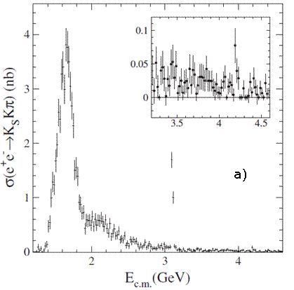
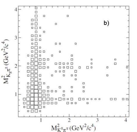
      Figure 1: a) The $e^{+}e^{-}\rightarrow K^{0}_{S}K^{\pm}\pi^{\mp}$ cross section measured by BaBar. b) Dalitz plot of the $e^{+}e^{-}\rightarrow K^{0}_{S}K^{\pm}K^{\mp}$ reaction: squared invariant masses of the $(K^{0}_{S}\pi^{\pm})$ versus the $(K^{\pm}\pi^{\mp})$ systems.

      From the inspection of the Dalitz plot shown in Fig. 1(b), which is fairly asymmetric, it is evident that the main contribution to the intermediate state is given by $K^{\ast}(892)^{\pm}K^{\mp}$ and $K^{\ast}(892)^{0}K^{0}_{S}$ and, at masses above 2 GeV, by $K^{\ast}_{2}(1430)^{\pm}K^{\mp}$ and $K^{\ast}_{2}(1430)^{0}K^{0}_{S}$. A Dalitz plot analysis was performed [3] to extract the isovector and isoscalar contributions to the cross section: interference effects model differently the production of charged and neutral $K^{\ast}$, which is mirrored in the asymmetry of the Dalitz plot. The dominant component was found to be the isoscalar one, with a clear resonant behavior to be identified with the mentioned $\phi(1680)$, while a broad contribution of marginal importance, that could be identified as the $\rho(1450)$, emerged from the fit.

   2. Measurement of $e^{+}e^{-}\rightarrow K^{+}K^{-}\pi^{0}$ Cross Section

      As the previous analysis, also in this case the main target was the possible identification of the Y(4260) state [3]. The trend of the measured cross section, reported in Fig. 2(a), shows even less evidence than in the previous case for the existence of an event excess, and again only un upper limit could be quoted for the decay branching ratio to this channel times the electronic width of the tentative signal, 0.6 eV at 90% C.L. A clear indication for $J/\psi$ production emerges from the cross section, whose maximum, $\sim 1$ nb, is reached at about 1.7 GeV.

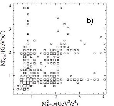
      Figure 2: a) The $e^{+}e^{-}\rightarrow K^{+}K^{-}\pi^{0}$ cross section measured by BaBar. b) Dalitz plot of the $e^{+}e^{-}\rightarrow K^{+}K^{-}\pi^{0}$ reaction: squared invariant masses of the $(K^{-}\pi^{0})$ versus the $(K^{+}\pi^{0})$ systems.

      The reaction Daliz plot, shown in Fig. 2, differently from the previous analysis is symmetric and features a dominant production of the final state through $K^{\ast}(892)^{\pm}K^{\mp}$ and $K^{\ast}_{2}(1430)^{\pm}K^{\mp}$. Selecting the $K^{+}K^{-}$ invariant mass system in the $\phi(1020)$ mass window, the $\phi\pi^{0}$ system could be studied: even if the available statistics was limited, as can be seen by the green points in Fig. 3, some indications for the existence of stuctures like $\rho(1700)/\rho(1900)$, observed as a dip, and a possible enhancement at about 1480 MeV (a possible hint for the long-sought isospin 1 $C(1480)$? [4]) are present.

      

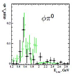
      Figure 3: $(\phi\pi^{0})$ cross section for events selected from the $e^{+}e^{-}\rightarrow K^{+}K^{-}\pi^{0}$ reaction (green points) and from the $e^{+}e^{-}\rightarrow K^{0}_{S}K^{0}_{L}\pi^{0}$ reaction (black points).

   3. Measurement of $e^{+}e^{-}\rightarrow K^{0}_{S}K^{0}_{L}\pi^{0}$ Cross Section

      Fig. 4 shows the trend of the $e^{+}e^{-}\rightarrow K^{0}_{S}K^{0}_{L}\pi^{0}$ cross section for this channel [5], whose maximum is about 3 nb corresponding to the excitation energy of the $\phi(1680)$. The systematic uncertainty of the measurement is 10% at the peak, and increases up to 30% at 3 GeV. For the first time a clear signal of $J/\psi$ is observed in the $K^{0}_{S}K^{0}_{L}\pi^{0}$ decay channel. The dominant intermediate state is $K^{\ast}(892)^{0}K^{0}$, which almost saturates the channel intensity: a clear signal is obtained for $K^{\ast}(892)^{0}$ for the combinations with both $K^{0}_{S}$ and $K^{0}_{L}$. Some hints for the production of the $K^{\ast}_{2}(1430)^{0}K^{0}$ are also observed.

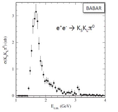
      Figure 4: The $e^{+}e^{-}\rightarrow K^{0}_{S}K^{0}_{L}\pi^{0}$ cross section measured by BaBar.

      The invariant mass of the $\phi(1020)\pi^{0}$ system, with the $\phi(1020)$ selected through its $K^{0}_{S}K^{0}_{L}$ decay, is shown by the black points in Fig. 3: even in this case some hints for a resonant activity at about 1.6 GeV can be observed, which could be a signature for an isospin 1 exotic structure.

4. Four Particles Final States

   1. Measurement of $e^{+}e^{-}\rightarrow K^{0}_{S}K^{0}_{L}\pi^{+}\pi^{-}$ sross section

      In the $e^{+}e^{-}\rightarrow K^{0}_{S}K^{0}_{L}\pi^{+}\pi^{-}$ channel the contribution of the background, coming both from ISR and non-ISR multihadronic events, is rather sizeable. Also the systematic uncertainty of the cross section, shown in Fig. 5(a), is larger, rising from about 10% at the peak, about 1 nb at $\sim$2 GeV, to 30% at 2.5–3 GeV, and up to 100% for energies in the center of mass larger than 3.4 GeV [6]. A clean signal of $J/\psi$ can be observed.

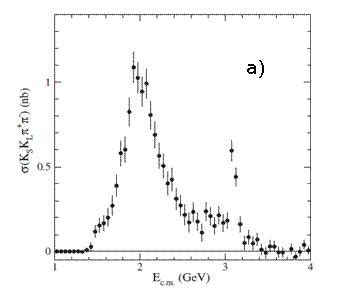
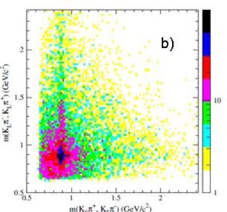
      Figure 5: a) The $e^{+}e^{-}\rightarrow K^{0}_{S}K^{0}_{L}\pi^{+}\pi^{-}$ cross section measured by BaBar. b) Scatter plot of the $e^{+}e^{-}\rightarrow K^{0}_{S}K^{0}_{L}\pi^{+}\pi^{-}$ reaction: invariant masses of the $(K^{0}_{L}\pi^{\mp})$ versus the $(K^{0}_{S}\pi^{+})$ systems.

      From the reaction scatter plot, shown in Fig. 5(b), clear bands of $K^{\ast}(892)^{\pm}$ can be observed with a weak indication for $K^{\ast}_{2}(1430)^{\pm}$. A strong correlated production of $K^{\ast}(892)^{+}K^{\ast}(892)^{-}$ and $K^{\ast}(892)^{\pm}K^{\ast}_{2}(1430)^{\mp}$ appears.

   2. Measurement of $e^{+}e^{-}\rightarrow K^{0}_{S}K^{0}_{S}\pi^{+}\pi^{-}$ Cross Section

      The cross section for the $e^{+}e^{-}\rightarrow K^{0}_{S}K^{0}_{S}\pi^{+}\pi^{-}$ reaction features a maximum of about 0.5 nb, affected by a 5% error, at about 2 GeV [6] (see Fig. 6(a)). From the inspection of the scatter plot shown in Fig.  6(b) one can note a clear correlated production of $K^{\ast}(892)$, dominant below 2.5 GeV, and a mild indication for $K^{\ast}_{2}(1430)^{\pm}$. There is basically no correlated production of $K^{\ast}(892)^{\pm}K^{\ast}_{2}(1430)^{\mp}$, and just a small strenght for the $K^{\ast}_{2}(1430)^{\pm}K_{S}\pi^{\mp}$ intermediate state can be observed.

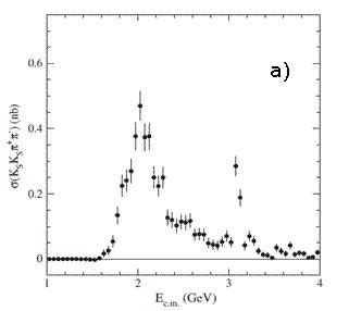
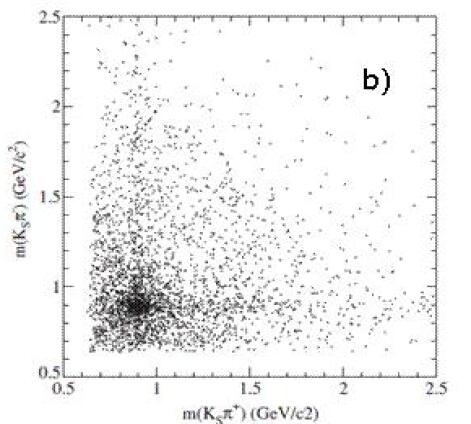
      Figure 6: a) The $e^{+}e^{-}\rightarrow K^{0}_{S}K^{0}_{S}\pi^{+}\pi^{-}$ cross section measured by BaBar. b) Scatter plot of the $e^{+}e^{-}\rightarrow K^{0}_{S}K^{0}_{S}\pi^{+}\pi^{-}$ reaction: invariant masses of the $(K^{0}_{S}\pi^{-})$ versus the $(K^{0}_{S}\pi^{\mp})$ systems.

   3. Measurement of $e^{+}e^{-}\rightarrow K^{+}K^{-}\pi^{+}\pi^{-}$ Cross Section

      The cross section for this channel was measured several years ago by the DM1 Experiment [7], up to an energy of about 2.5 GeV: the comparison with the most recent measurements by BaBar [8], reported in Fig. 7(a), show that the early results, represented by the red open points, were most probably overestimated and affected by a sizeable systematic error. In the present case, the systematic uncertainty was evaluated as about 20% below 1.6 GeV, lowering to as little as 2% in the region around 2 GeV to rise again up to about 10% above 3 GeV. Narrow peaks from the formation of charmonium ($J/\psi$ and $\psi(2S)$) and possibly other structures which may be produced upon the opening of reaction thresholds are visible in the cross section, whose maximum is $\sim$4 nb at about 2 GeV.

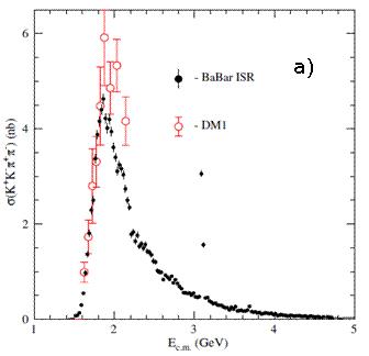
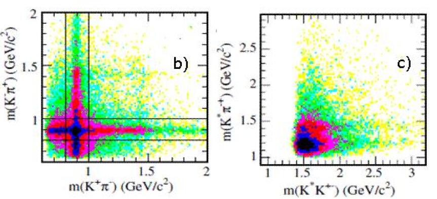
      Figure 7: a) The $e^{+}e^{-}\rightarrow K^{+}K^{-}\pi^{+}\pi^{-}$ cross section measured by BaBar and DM1 (red open points [7]). b)-c) Scatter plots of the $e^{+}e^{-}\rightarrow K^{+}K^{-}\pi^{+}\pi^{-}$ reaction: b) invariant masses of the $(K^{-}\pi^{+})$ versus the $(K^{+}\pi^{-})$ systems, c) invariant masses of the $(K^{\ast}\pi^{\mp})$ versus the $(K^{\ast}K^{\pm})$ systems.

      The scatter plots of the invariant masses of particles’ pairs are displayed in Fig. 7(b) and c): they show the presence of plenty of intermediate states, with clear signatures from $K^{\ast}(892)^{0}$ and $K^{\ast}_{2}(1430)^{0}$, and the evidence, seen as horizontal bands in Fig. 7(c), of contributions from the $K_{1}(1270)$ and $K_{1}(1400)$ axial excitations decaying in $K^{\ast}(892)^{0}\pi^{\pm}$. The $(\pi^{+}\pi^{-})$ invariant mass spectrum (not shown) displays a clear enhancement corresponding to the $\rho(770)$ signal, which can be an evidence for the possible decay of the two axial mesons in $K\rho$. No other signal is observed in the $(\pi^{+}\pi^{-})$ system.

   4. Measurement of $e^{+}e^{-}\rightarrow K^{+}K^{-}\pi^{0}\pi^{0}$ Cross Section

      The cross section for the $e^{+}e^{-}\rightarrow K^{+}K^{-}\pi^{0}\pi^{0}$ reaction is shown in Fig. 8: it does not exceed 1 nb and the maximum is located around 2 GeV [8]. A clear charmonium signal is present. The systematic uncertainty of the cross section is about 7% at low energies, rising to 18% above 3 GeV. The dominant contribution to the intermediate states is played by $K^{\ast}(892)$.

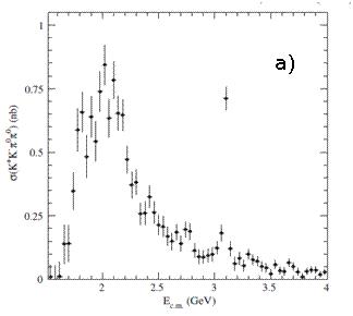
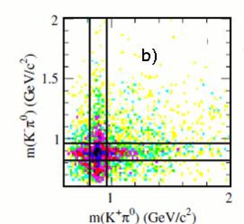
      Figure 8: a) The $e^{+}e^{-}\rightarrow K^{+}K^{-}\pi^{0}\pi^{0}$ cross section measured by BaBar. b) Scatter plot of the $e^{+}e^{-}\rightarrow K^{+}K^{-}\pi^{0}\pi^{0}$ reaction: invariant masses of the $(K^{-}\pi^{0})$ versus the $(K^{+}\pi^{0})$ systems.

      The corresponding scatter plot of the invariant masses of the $(K^{-}\pi^{0})$ versus the $(K^{+}\pi^{0})$ systems is shown in Fig. 8(b), and displays a clear correlated production of $K^{\ast}(892)$ pairs as well as $K^{\ast}(892)^{+}K^{\ast}_{2}(1430)^{-}$; however, no evidence of resonant production in the three particles systems $(K^{+}K^{-}\pi^{0})$ or $(K^{\pm}\pi^{0}\pi^{0})$ can be observed.

   5. Measurement of $e^{+}e^{-}\rightarrow K^{0}_{S}K^{0}_{L}\pi^{0}\pi^{0}$ Cross Section

      The $e^{+}e^{-}\rightarrow K^{0}_{S}K^{0}_{L}\pi^{0}\pi^{0}$ cross section was found to be relatively small, reaching at most 0.6 nb at its maximum at $\sim$ 1.7 GeV, with a systematic uncertainty of about 25% at the peak, increasing to 60% above 2 GeV. For the first time the $J/\phi$ was observed in this decay channel [9]. The cross section is shown in Fig. 9.

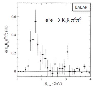
      Figure 9: The $e^{+}e^{-}\rightarrow K^{0}_{S}K^{0}_{L}\pi^{0}\pi^{0}$ cross section measured by BaBar.

      While the dominant contribution to the intermediate states is played, as usual, by $K^{\ast}(892)$, there is no significant contribution to this channel of the correlated production of two $K^{\ast}$’s.

   6. Measurement of $e^{+}e^{-}\rightarrow K^{0}_{S}K^{\pm}\pi^{\mp}\pi^{0}$ Cross Section

      The $K^{0}_{S}K^{\pm}\pi^{\mp}\pi^{0}$ channel features a rich intermediate state composition [10]. Apart from the clean $J/\psi$ signal, whose strength exceeds the maximum of the cross section (about 2 nb, measured with a systematic uncertainty of $\sim$ 7% below 3 GeV), as shown in Fig. 10(a), several intermediate states can be observed from the inspection of the scatter plots reported in Fig. 10(b).

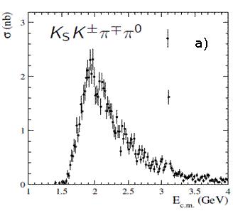
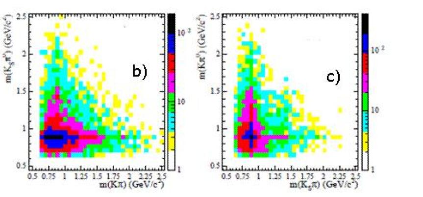
      Figure 10: a) The $e^{+}e^{-}\rightarrow K^{0}_{S}K^{\pm}\pi^{\mp}\pi^{0}$ cross section measured by BaBar. b)-c) Scatter plots of the $e^{+}e^{-}\rightarrow K^{0}_{S}K^{\pm}\pi^{\mp}\pi^{0}$ reaction: b) invariant masses of the $(K^{0}_{S}\pi^{0})$ versus the $(K\pi)$ systems, c) invariant masses of the $(K\pi^{0})$ versus the $(K^{0}_{S}\pi)$ systems.

      The dominant ones are $K^{\ast}(892)\overline{K}\pi$ and $K^{0}_{S}K^{\pm}\rho^{\mp}$. This last channel is partly fed by the decay of the axial excitations $K_{1}(1270),\;K_{1}(1400)$ and $K_{1}(1650)$. The correlated $K^{\ast}\overline{K}$ production is relatively small (less than 15%), and almost saturated by the $K^{\ast+}K^{\ast-}$ charged mode.

5. Summary and Conclusions

   The total cross sections for $e^{+}e^{-}$ annihilation in $K\overline{K}\pi$ and $K\overline{K}2\pi$, thanks to the new BaBar measurements described above, can now be evaluated basically without any model assumptions, nor resorting to isospin symmetry relationships [11]. In the comparison of all the exclusive hadronic cross section measured by BaBar, the dominant contribution is played by full pionic channels: in particular between 1 and 2 GeV the four pion production dominates, while above 2 GeV the six pion production gives the largest contribution.

   Adding up all channels with kaons and a total of three particles in the final state, the cross section amounts to about 12% of the total hadronic cross section, at the maximum located at about 1.6–1.7 GeV.

   Concerning the four particle final state, the largest contribution is played by the $K^{+}K^{-}\pi^{+}\pi^{-}$ and $K^{0}_{S}K^{+}\pi^{-}\pi^{0}$ channels; the total cross section at 2 GeV is about 1/4 of the total hadronic cross section.

   The precise knowledge of the hadronic cross sections, for which BaBar contributed providing an unprecedented bulk of new results in more than 20 channels (including those with pions only and $\eta$’s not described in this paper), could improve the accuracy of new evaluations of the $a^{had,LO}_{\mu}$ term of the muon anomalous magnetic moment by 21% as compared to previous assessments [12].

   Moreover, the program of ISR measurements with BaBar could provide new interesting information about hadronization at low energies and the properties of the light meson spectrum.

   New more precise results are awaited soon from the application of this technique at the new generation of charm and B-Factories.

4 List of Participants of PKI2018 Workshop

• Miguel Albaladejo Serrano, U. Murcia <albaladejo_at_um.es>

• Moskov Amaryan, ODU <mamaryan_at_odu.edu>

• Alexander Austregesilo, JLab <aaustreg_at_jlab.org>

• Marouen Baalouch, ODU/JLab <baalouh_at_jlab.com

• Ted Barnes, DOE-NP <ted.barnes_at_science.doe.gov>

• Silas R. Beane, University of Washington <silas_at_uw.edu>

• Raul Briceno, ODU <rbriceno_at_jlab.org>

• Eugene Chudakov, JLab <gen_at_jlab.org>

• Michael Döring, GW/JLab <doring_at_gwu.edu>

• Josef Dudek, W&M <dudek_at_jlab.org>

• Robert Edwards, JLab <edwards_at_jlab.org>

• Rolf Ent, JLab <ent_at_jlab.org>

• Denis Epifanov, BINP, NSU <d.a.epifanov_at_inp.nsk.su>

• Stuart Fegan, GW/JLab <sfegan_at_jlab.org>

• Alessandra Filippi, INFN Torino <filippi_at_to.infn.it>

• José Goity, JLab <goity_at_jlab.org>

• Boris Grube, Technical University Munich <bgrube_at_tum.de>

• Zhihui Guo, Hebei Normal University <zhguo_at_hebtu.edu.cn>

• Avetik Hayrapetyan, JLU Giessen <Avetik.Hayrapetyan_at_uni-giessen.de>

• Charles E. Hyde, ODU <chyde_at_odu.edu>

• Vyacheslav Ivanov, Budker Institute of Nuclear Physics <vyacheslav-lvovich-ivanov_at_mail.ru>

• Tanjib Khan, W&M <mkhan01_at_email.wm.edu>

• Chan Kim, GW <kimchanwook_at_gwu.edu>

• Bastian Kubis, Bonn U. <kubis_at_hiskp.uni-bonn.de>

• Luka Leskovec, University of Arizona <leskovec_at_email.arizona.edu>

• Wenliang Li, W&M <wli08_at_wm.edu>

• Pok Man Lo, University of Wroclaw <pmlo_at_ift.uni.wroc.pl>

• Maxim Mai, GW <maxim.mai_at_posteo.net>

• Vincent Mathieu, JLab <vmathieu_at_jlab.org>

• Curtis Meyer, CMU <cmeyer_at_cmu.edu>

• Daniel G. Mohler, Helmholtz-Institut Mainz <damohler_at_uni-mainz.de>

• Colin Morningstar, CMU <colin-morningstar_at_cmu.edu>

• Bachir Moussallam, Universite Paris-Sud <moussall_at_ipno.in2p3.fr>

• Leonid Nemenov, JINR <leonid.nemenov_at_cern.ch>

• José Antonio Oller, Universidad de Murcia <oller_at_um.es>

• Bilas K. Pal, University of Cincinnati <palbs_at_ucmail.uc.edu>

• Antimo Palano, INFN and University of Bari <antimo.palano_at_ba.infn.it>

• Emilie Passemar, IU/JLab <epassema_at_indiana.edu>

• José R. Pelaez, Universidad Complutense de Madrid <jrpelaez_at_fis.ucm.es>

• William Phelps, GW <wphelps_at_jlab.org>

• Alessandro Pilloni, JLab <pillaus_at_jlab.org>

• Jianwei Qiu, JLab <jqiu_at_jlab.org>

• David Richards, JLab <dgr_at_jlab.org>

• James L. Ritman, Forschungszentrum Jülich GmbH <j.ritman_at_fz-juelich.de>

• Torry Roak, ODU <roark_at_jlab.org>

• Patrizia Rossi, JLab <rossi_at_jlab.org>

• Jacobo Ruiz de Elvira, Bern University <elvira_at_itp.unibe.ch>

• Akaki Rusetsky, University of Bonn <rusetsky_at_hiskp.uni-bonn.de>

• Amy M. Schertz, W&M <amschertz_at_email.wm.edu>

• Rafael Silva Coutinho, Universität Zürich <rsilvaco_at_cern.ch>

• Justin R. Stevens, W&M <jrstevens01_at_wm.edu>

• Igor Strakovsky, GWU <igor_at_gwu.edu>

• Adam Szczepaniak, IU/JLab <aszczepa_at_indiana.edu>

• Tyler Viducic, W&M <tyler.viducic_at_gmail.com>

• Nilanga Wickramaarachchi, ODU <nwick001_at_odu.edu>

References

- [1] M. Amaryan, Ulf-G. Meißner, C. Meyer, J. Ritman, and I. Strakovsky, eds., Mini-Proceedings, Workshop on Physics with Neutral Kaon Beam at JLab (KL2016); arXiv:1604.02141 [hep–ph]. M. Amaryan, E. Chudakov, K. Rajagopal, C. Ratti, J. Ritman, and I. Strakovsky, eds., Mini-Proceedings, Workshop on Excited Hyperons in QCD Thermodynamics at Freeze-Out (YSTAR2016); arXiv:1701.07346 [hep–ph].
- [2] M. Amaryan, E. Chudakov, K. Rajagopal, C. Ratti, J. Ritman, and I. Strakovsky, eds., Mini-Proceedings, Workshop on Excited Hyperons in QCD Thermodynamics at Freeze-Out (YSTAR2016); arXiv:1701.07346 [hep–ph].
- [3] T. Horn, C. Keppel, C. Munoz-Camacho, and I. Strakovsky, eds., Mini-Proceedings, Workshop on High-Intensity Photon Sources (HIPS2017); arXiv:1704.00816 [nucl–ex].

References

- [1] M. Amaryan, Ulf-G. Meißner, C. Meyer, J. Ritman, and I. Strakovsky, eds., Mini-Proceedings, Workshop on Physics with Neutral Kaon Beam at JLab (KL2016); arXiv:1604.02141 [hep–ph].
- [2] M. Amaryan, E. Chudakov, K. Rajagopal, C. Ratti, J. Ritman, and I. Strakovsky, eds., Mini-Proceedings, Workshop on Excited Hyperons in QCD Thermodynamics at Freeze-Out (YSTAR2016); arXiv:1701.07346 [hep–ph].
- [3] T. Horn, C. Keppel, C. Munoz-Camacho, and I. Strakovsky, eds., Mini-Proceedings, Workshop on High-Intensity Photon Sources (HIPS2017); arXiv:1704.00816 [nucl–ex].
- [4] S. Adhikari et al. [GlueX Collaboration], arXiv:1707.05284 [hep-ex].
- [5] H. Seraydaryan et al. [CLAS Collaboration], Phys. Rev. C 89, no. 5, 055206 (2014).
- [6] A. I. Titov and T. S. H. Lee, Phys. Rev. C 67, 065205 (2003).
- [7] G. Mcclellan, N. B. Mistry, P. Mostek, H. Ogren, A. Osborne, J. Swartz, R. Talman, and G. Diambrini-Palazzi, Phys. Rev. Lett. 26, 1593 (1971).
- [8] D. Androic et al. [G0 Collaboration], Nucl. Instrum. Meth. A 646, 59 (2011).
- [9] W. E. Cleland, B. Goz, D. Freytag, T. J. Devlin, R. J. Esterling and K. G. Vosburgh, Phys. Rev. D 12, 1247 (1975).
- [10] G. W. Brandenburg et al., Phys. Rev. D 7, 708 (1973).
- [11] B. C. Jackson, Y. Oh, H. Haberzettl and K. Nakayama, Phys. Rev. C 91, no. 6, 065208 (2015).
- [12] C. Patrignani et al. [Particle Data Group], Chin. Phys. C 40, no. 10, 100001 (2016).
- [13] K. T. Chao, N. Isgur and G. Karl, Phys. Rev. D 23, 155 (1981).
- [14] C. M. Jenkins et al., Phys. Rev. Lett. 51, 951 (1983).
- [15] R. G. Edwards et al. [Hadron Spectrum Collaboration], Phys. Rev. D 87, no. 5, 054506 (2013).
- [16] G. P. Engel et al. [BGR Collaboration], Phys. Rev. D 87, no. 7, 074504 (2013).
- [17] H. Takahashi, Nucl. Phys. A 914, 553 (2013).

References

- [1] C. Morningstar, J. Bulava, B. Singha, R. Brett, J. Fallica, A. Hanlon, and B. Hörz, Nucl. Phys. B 924, 477 (2017).
- [2] C. Morningstar, J. Bulava, B. Fahy, J. Foley, Y.C. Jhang, K.J. Juge, D. Lenkner, and C.H. Wong, Phys. Rev. D 88, 014511 (2013).
- [3] R. Brett, J. Bulava, J. Fallica, A. Hanlon, B. Hörz, and C. Morningstar, arXiv:1802.03100 [hep-lat] (2018).
- [4] C. Morningstar, J. Bulava, J. Foley, K. J. Juge, D. Lenkner, M. Peardon, and C. H. Wong, Phys. Rev. D 83, 114505 (2011).
- [5] S. Prelovsek, L. Leskovec, C. B. Lang, and D. Mohler, Phys. Rev. D88, 054508 (2013).
- [6] D. J. Wilson, J. J. Dudek, R. G. Edwards, and C. E. Thomas, Phys. Rev. D91, 054008 (2015).
- [7] G. S. Bali et al., Phys. Rev. D93, 054509 (2016).
- [8] M. Döring and Ulf-G. Meißner, JHEP 1201, 009 (2012).
- [9] J. Bulava, B. Fahy, B. Hörz, K. J. Juge, C. Morningstar, and C. H. Wong, Nucl. Phys. B 910, 842 (2016).
- [10] C. W. Andersen, J. Bulava, B. Hörz, and C. Morningstar, Phys. Rev. D 97, 014506 (2018).

References

- [1] G. Ecker, Prog. Part. Nucl. Phys. 35 (1995) 1.
- [2] B. Ananthanarayan, G. Colangelo, J. Gasser, and H. Leutwyler, Phys. Rept. 353 (2001) 207.
- [3] J.P. Ader, C. Meyers, and B. Bonnier Phys. Lett. B 46 (1973) 403.
- [4] C. B. Lang, Nuovo Cim. A 41 (1977) 73.
- [5] N. Johannesson and G. Nilsson, Nuovo Cim. A 43 (1978) 376.
- [6] P. Buttiker, S. Descotes-Genon, and B. Moussallam, talk given at QCD-03 conference, 2-9 July 2003, Montpellier; hep-ph/0310045.
- [7] V. Bernard, N. Kaiser, and Ulf-G. Meißner, Phys. Rev. D 43 (1991) 2757.
- [8] V. Bernard, N. Kaiser, and Ulf-G. Meißner, Nucl. Phys. B 357 (1991) 129
- [9] V. Bernard, N. Kaiser, and Ulf-G. Meißner, Nucl. Phys. B 364 (1991) 283.
- [10] E. M. Aitala et al. (E791 Collaboration), Phys. Rev. Lett. 89 (2002) 121801.
- [11] J. Z. Bai et al. (BES Collaboration), hep-ex/0304001.
- [12] S. Descotes-Genon and B. Moussallam, Eur. Phys. J. C 48 (2006) 553.
- [13] H. Q. Zheng et al. Nucl. Phys. A 733, 235 (2004).
- [14] J. R. Pelaez and A. Rodas, Phys. Rev. D 93, 074025 (2016).
- [15] A. Palano and M. R. Pennington, arXiv:1701.04881,
- [16] V. Bernard, M. Oertel, E. Passemar, and J. Stern, Phys. Rev. D 80 (2009) 034034.
- [17] M. Antonelli et. al., Eur. Phys. J. C 69 (2010) 399.
- [18] D. Aston et al., Nucl. Phys. B 296, 493 (1988).
- [19] F. Schweingruber, M. Derrick, T. Fields, D. Griffiths, L. G. Hyman, R.J. Jabbur, J. Lokan, R. Ammar, R.E.P. Davis, W. Kropac, and J. Mott, Phys. Rev. 166 (1968) 1317.
- [20] G. Ranft et al. [Birmingham-Glasgow-London (I.C.)-Mtinchen-Oxford-Rutherford Laboratory Collaboration], Nuovo Cimento 53A (1968) 522.
- [21] J. H. Friedman and R. R. Ross, Phys. Rev. Lett. 16 (1966) 485.
- [22] Birmingham-Glasgow-Oxford Collaboration, private communication; CERN Topical Conf. on high-energy collisions of hadrons, Vol. II, p. 121 (1968).
- [23] H. Al Ghoul et al. [GlueX Collaboration], AIP Conf. Proc. 1735, 020001 (2016).

References

- [1] J. P. Lees et al. [BaBar Collaboration], Phys. Rev. D 89, no. 11, 112004 (2014).
- [2] J. P. Lees et al. [BaBar Collaboration], Phys. Rev. D 93, 012005 (2016).
- [3] S. Eidelman et al. [Particle Data Group], Phys. Lett. B 592, no. 1-4, 1 (2004).
- [4] E. M. Aitala et al. [E791 Collaboration], Phys. Rev. D 73, 032004 (2006); Erratum: [Phys. Rev. D 74, 059901 (2006)].
- [5] D. Aston et al., Nucl. Phys. B 296, 493 (1988).
- [6] K. M. Watson, Phys. Rev. 88, 1163 (1952).
- [7] P. Estabrooks et al., Nucl. Phys. B133, 490 (1978).
- [8] A. Palano and M. R. Pennington, arXiv:1701.04881 [hep-ph].
- [9] P. Buettiker, S. Descotes-Genon and B. Moussallam, Eur. Phys. J. C 33, 409 (2004).
- [10] A. V. Anisovich and A. V. Sarantsev, Phys. Lett. B 413, 137 (1997).
- [11] J. P. Lees et al. [BaBar Collaboration], Phys. Rev. D 95, no. 7, 072007 (2017).
- [12] C. Zemach, Phys. Rev. 133, B1201 (1964).
- [13] C. Dionisi et al., Nucl. Phys. B 169, 1 (1980).
- [14] C. Patrignani et al. (Particle Data Group), Chin. Phys. C 40, 100001 (2016) and 2017 update.

References

- [1] C. Patrignani et al. [Particle Data Group], Chin. Phys. C 40, 100001 (2016).
- [2] D. Ebert, R. N. Faustov, and V. O. Galkin, Phys. Rev. D 79, 114029 (2009).
- [3] C. Daum et al. [ACCMOR Collaboration], Nucl. Phys. B 187 (1981) 1.
- [4] D. Aston et al. [LASS Collaboration], Nucl. Phys. B 292, 693 (1987).
- [5] D. Aston et al. [LASS Collaboration], SLAC-PUB-5236, in proceedings of the 1990 Meeting of the Division of Particles and Fields of the American Physical Society (DPF90), Houston, USA, January 3–6, 1990.
- [6] P. Jasinski, Ph.D. Thesis, Universität Mainz, January 2012.
- [7] P. Jasinski [COMPASS Collaboration], in Proceedings of the XIV International Conference on Hadron Spectroscopy (hadron2011), Munich, Germany, 2011, eConf C110613, 279 (2011).
- [8] C. Adolph et al. [COMPASS Collaboration], Phys. Rev. D 95, 032004 (2017).
- [9] S. U. Chung and T. L. Trueman, Phys. Rev. D 11, 633 (1975)
- [10] R. Akhunzyanov et al. [COMPASS Collaboration], [arXiv:1802.05913].
- [11] F. Krinner, D. Greenwald, D. Ryabchikov, B. Grube, and S. Paul, [arXiv:1710.09849].
- [12] W. K. H. Panofsky and W. Wenzel, Rev. Sci. Instrum. 27, 967 (1956).
- [13] P. Bernard, P. Lazeyras, H. Lengeler, and V. Vaghin, CERN-68-29 (1968).
- [14] A. Citron, G. Dammertz, M. Grundner, L. Husson, R. Lehm, H. Lengeler, D. E. Plane, and G. Winkler, Nucl. Instrum. Meth. 155, 93 (1978)
- [15] L. Gatignon, Physics Beyond Colliders Kickoff Workshop, CERN, 6–7 September 2016.
- [16] J. Bernhard, Workshop on Dilepton Productions with Meson and Antiproton Beams, ECT*, Trento, Italy, 6–10 November 2017.

References

- [1] S. Kurokawa and E. Kikutani, Nucl. Instrum. Methods Phys. Res. Sect. A 499, 1 (2003), and other papers included in this Volume; T. Abe et al., Prog. Theor. Exp. Phys. 2013, 03A011 (2013). and references therein.
- [2] A. Abashian et al. (Belle Collaboration), Nucl. Instrum. Methods Phys. Res. Sect. A 479, 117 (2002); also see the detector section in J. Brodzicka et al., Prog. Theor. Exp. Phys. 2012, 04D001 (2012).
- [3] Z. Natkaniec et al. (Belle SVD2 Group), Nucl. Instrum. Methods Phys. Res. Sect. A 560, 1 (2006).
- [4] B. Aubert et al. (BaBar Collaboration), Phys. Rev. Lett. 99, 221801 (2007).
- [5] R. Aaij et al. (LHCb Collaboration), Phys. Rev. Lett. 112, 011801 (2014).
- [6] R. Aaij et al. (LHCb Collaboration), Phys. Rev. D 90, 112004 (2014).
- [7] B. Bhattacharya, M. Gronau, and J. L. Rosner, Phys. Lett. B 726, 337 (2013).
- [8] I. Bediaga, T. Frederico, and O. Louren?, Phys. Rev. D 89, 094013 (2014).
- [9] C.-L. Hsu et al. (Belle Collaboration), Phys. Rev. D 96, 031101 (2017).
- [10] S. K. Choi et al. (Belle Collaboration), Phys. Rev. Lett. 91, 262001 (2003).
- [11] C. Patrignani et al. (Particle Data Group), Chin. Phys. C 40, 100001 (2016).
- [12] R. Aaij et al. (LHCb Collaboration), Phys. Rev. Lett. 115, 072001 (2015).
- [13] R. Zhu and C. F. Qiao, Phys. Lett. B 756, 259 (2016).
- [14] V. Kopeliovich and I. Potashnikova, arXiv:1510.05958 [hep-ph].
- [15] R. F. Lebed, Phys. Rev. D 92, 114030 (2015).
- [16] T. Mibe et al. (LEPS Collaboration), Phys. Rev. Lett. 95, 182001 (2005).
- [17] B. Dey et al. (CLAS Collaboration), Phys. Rev. C 89, 055208 (2014); Phys. Rev. C 90, 019901 (2014).
- [18] R. F. Lebed, Phys. Rev. D 92, 114006 (2015).
- [19] B. Pal et al. (Belle Collaboration), Phys. Rev. D 96, 051102 (2017).
- [20] Y. Amhis et al. (Heavy Flavor Averaging Group), arXiv:1612.07233 [hep-ex].
- [21] M. Ablikim et al. (BESIII Collaboration), Phys. Rev. Lett. 116, 052001 (2016).
- [22] H. J. Lipkin, Nucl. Phys. Proc. Suppl. 115, 117 (2003).
- [23] D. N. Gao, Phys. Lett. B 645, 59 (2007).
- [24] J. M. Link et al. (FOCUS Collaboration), Phys. Lett. B 624, 166 (2005).
- [25] S. B. Yang et al. (Belle Collaboration), Phys. Rev. Lett. 117, 011801 (2016).
- [26] R. Aaij et al. (LHCb Collaboration), arXiv:1711.01157 [hep-ex].
- [27] A. Zupanc et al. (Belle Collaboration), Phys. Rev. Lett. 113, 042002 (2014).
- [28] M. Gronau and D. London, Phys. Lett. B 253, 483 (1991).
- [29] M. Gronau and D. Wyler, Phys. Lett. B 265, 172 (1991).
- [30] D. Atwood, I. Dunietz, and A. Soni, Phys. Rev. D 63, 036005 (2001).
- [31] A. Giri, Y. Grossman, A. Soffer, and J. Zupan, Phys. Rev. D 68, 054018 (2003).
- [32] A. Poluektov et al. (Belle Collaboration), Phys. Rev. D 81, 112002 (2010).
- [33] H. Aihara et al. (Belle Collaboration), Phys. Rev. D 85, 112014 (2012).
- [34] A. Bondar and A. Poluektov, Eur. Phys. J. C 55, 51 (2008).
- [35] R. A. Briere et al. (CLEO Collaboration), Phys. Rev. D 80, 032002 (2009).
- [36] J. Libby et al. (CLEO Collaboration), Phys. Rev. D 82, 112006 (2010).

References

- [1] A. J. Bevan et al. [BaBar and Belle Collaborations], Eur. Phys. J. C 74, 3026 (2014).
- [2] W. Fetscher and H. J. Gerber, Adv. Ser. Direct. High Energy Phys. 14, 657 (1995).
- [3] A. Pich, Adv. Ser. Direct. High Energy Phys. 15, 453 (1998).
- [4] E. Gamiz, M. Jamin, A. Pich, J. Prades, and F. Schwab, Phys. Rev. Lett. 94, 011803 (2005).
- [5] D. Aston et al. (LASS Collaboration), Nucl. Phys. B 296, 493 (1988).
- [6] S. Dobbs [GlueX Collaboration], PoS ICHEP 2016, 1243 (2017).
- [7] D. Delepine, G. Lopez Castro, and L. -T. Lopez Lozano, Phys. Rev. D 72, 033009 (2005).
- [8] J. H. Kuhn and E. Mirkes, Phys. Lett. B 398, 407 (1997).
- [9] D. Epifanov et al. [Belle Collaboration], Phys. Lett. B 654, 65 (2007).
- [10] M. Bischofberger et al. [Belle Collaboration], Phys. Rev. Lett. 107, 131801 (2011).
- [11] S. Ryu et al. [Belle Collaboration], Phys. Rev. D 89, 072009 (2014).
- [12] B. Aubert et al. [BaBar Collaboration], Phys. Rev. D 76, 051104 (2007).
- [13] B. Aubert et al. [BaBar Collaboration], Nucl. Phys. Proc. Suppl. 189, 193 (2009).
- [14] J. P. Lees et al. [BaBar Collaboration], Phys. Rev. D 85, 031102 (2012); Erratum: [Phys. Rev. D 85, 099904 (2012)].
- [15] W.-M. Yao et al., J. Phys. G 33, 1 (2006).
- [16] M. Finkemeier and E. Mirkes, Z. Phys. C 72, 619 (1996).
- [17] J. H. Kuhn and E. Mirkes, Phys. Lett. B 398, 407 (1997).
- [18] Y. Grossman, Nucl. Phys. B 426, 355 (1994).
- [19] S. Y. Choi, K. Hagiwara, and M. Tanabashi, Phys. Rev. D 52, 1614 (1995).
- [20] Y. M. Shatunov et al., Conf. Proc. C 0006262 (2000) 439.
- [21] D. Berkaev et al., Nucl. Phys. Proc. Suppl. 225-227 (2012) 303.

References

- [1] I. Caprini, G. Colangelo, and H. Leutwyler, Phys. Rev. Lett. 96 (2006) 132001.
- [2] R. Omnès, Nuovo Cim. 8 (1958) 316.
- [3] J. F. Donoghue, J. Gasser, and H. Leutwyler, Nucl. Phys. B 343 (1990) 341.
- [4] B. Hyams et al., Nucl. Phys. B 64 (1973) 134.
- [5] D. H. Cohen et al., Phys. Rev. D 22 (1980) 2595.
- [6] A. Etkin et al., Phys. Rev. D 25 (1982) 1786.
- [7] G. P. Lepage and S. J. Brodsky, Phys. Rev. D 22 (1980) 2157.
- [8] F. J. Yndurain et al., Phys. Lett. B 578 (2004) 99.
- [9] B. "Ananthanarayan et al., Phys. Lett. B 602 (2004) 218.
- [10] N. Noether, Mathematische Annalen, 82 (1921) 42.
- [11] V. Gülpers et al., Phys. Rev. D 89 (2014) 094503.
- [12] P. Estabrooks et al., Nucl. Phys. B 133 (1978) 490.
- [13] D. Aston et al., Nucl. Phys. B 296 (1988) 493.
- [14] M. Jamin et al., Nucl. Phys. B 622 (2002) 279.
- [15] M. Jamin et al., Phys. Rev. D 74 (2006) 074009.
- [16] M. Piccini [for NA48/2 Collaboration], Proceedings, 2017 European Physical Society Conference on High Energy Physics (EPS-HEP 2017): Venice, Italy, July 5-12, 2017; PoS EPS-HEP2017 (2018) 235.
- [17] D. Aston et al., Nucl. Phys. B 292 (1987) 693.
- [18] B. Moussallam, Eur. Phys. J. C 53 (2008) 401.
- [19] V. Bernard, JHEP, 06 (2014) 082.
- [20] D. Aoki et al., Eur. Phys. J. C 77 (2017) 112.
- [21] D. Epifanov et al. [Belle Collaboration], Phys. Lett. B 654 (2007) 65.
- [22] J. R. Peláez et al., Eur. Phys. J. C 77 (2017) 91.

References

- [1] P. Abbon et al. (COMPASS Collaboration), Nucl. Instrum. Meth. A 577, 455 (2007).
- [2] H. Al Ghoul et al. [GlueX Collaboration], AIP Conf. Proc. 1735, 020001 (2016).
- [3] D. I. Glazier, Acta Phys. Polon. Supp. B 8, 503 (2017).
- [4] M. Mikhasenko, B. Ketzer, and A. Sarantsev, Phys. Rev. D 91, 094015 (2015).
- [5] R. F. Lebed, R. E. Mitchell, and E. S. Swanson, Prog. Part. Nucl. Phys. 93, 143 (2017).
- [6] Feng-Kun Guo et al. arXiv:1705.00141 [hep-ph].
- [7] A. A. Alves et al. (LHCb Collaboration), JINST, 3, S08005 (2008).
- [8] S. Fang (for BESIII Collaboration), Nucl. Part. Phys. Proc. 273, 1949 (2016).
- [9] I. J. R. Aitchison and J. J. Brehm, Phys. Rev. D 17, 3072 (1978).
- [10] S. Adhikari et al. [GlueX Collaboration], arXiv:1707.05284 [hep-ex].
- [11] M. Amaryan, E. Chudakov, K. Rajagopal, C. Ratti, J. Ritman, and I. Strakovsky, eds., Mini-Proceedings, Workshop on Excited Hyperons in QCD Thermodynamics at Freeze-Out (YSTAR2016); arXiv:1701.07346 [hep–ph].
- [12] T. Horn, C. Keppel, C. Munoz-Camacho, and I. Strakovsky, eds., Mini-Proceedings, Workshop on High-Intensity Photon Sources (HIPS2017); arXiv:1704.00816 [nucl–ex].
- [13] M. Amaryan, Ulf-G. Meißner, C. Meyer, J. Ritman, and I. Strakovsky, eds., Mini-Proceedings, Workshop on Physics with Neutral Kaon Beam at JLab (KL2016); arXiv:1604.02141 [hep–ph].
- [14] C. B. Lang et al., JHEP, 04, (2014) 162.
- [15] C. B. Lang et al., Phys. Rev. D 95 (2017) 014510.
- [16] A. L. Kiratidis et al., Phys. Rev. D 95 (2017) 074507.
- [17] A. J. Woss et al., arXiv:1802.05580 [hep-lat].
- [18] S. R. Sharpe, arXiv:1707.04279 [hep–lat].
- [19] H.-W. Hammer et al., arXiv:1707.02176 [hep–lat].
- [20] H.-W. Hammer et al., arXiv:1706.07700 [hep–lat].
- [21] M. T. Hansen et al., arXiv:1704.08993 [hep–lat].
- [22] Peng Guo and V. Gasparian, arXiv:1701.00438 [hep–lat].
- [23] D. Agadjanov et al., JHEP, 06 (2016) 043.
- [24] M. T. Hansen and S. R. Sharpe, Phys. Rev. D 95 (2017) 034501.
- [25] M. T. Hansen and S. R. Sharpe, Phys. Rev. D 93 (2016) 096006.
- [26] M. T. Hansen and S. R. Sharpe, Phys. Rev. D 93 (2016) 014506.
- [27] M. T. Hansen and S. R. Sharpe, Phys. Rev. D 92 (2015) 114509.
- [28] Ulf-G. Meissner et al., Phys. Rev. Lett. 114 (2015) 091602.
- [29] K. Polejaeva and A. Rusetsky, Eur. Phys. J. A 67 (2012) 67.
- [30] M. Mai and M. Döring, Eur. Phys. J. A 53 (2017) 240.
- [31] R. A. Briceño, M. T. Hansen, and S. R. Sharpe, arXiv:1803.04169 [hep-lat].
- [32] M. Döring, H.-W. Hammer, M. Mai, J.-Y. Pang, A. Rusetsky, and J. Wu, arXiv:1802.03362 [hep-lat].
- [33] P. F. Bedaque and H. W. Greahammer, Nucl. Phys. A 671 (2000) 357.
- [34] M. Mai et al., arXiv:1706.06118 [nucl–th].
- [35] M. Döring et al., Eur. Phys. J. A 47 (2011) 163.

References

- [1] K. Hagiwara, R. Liao, A.D. Martin, D. Nomura, and T. Teubner, J. Phys. G 38, 085003 (2011).
- [2] G.W. Bennett et al. (Muon g-2 Collaboration), Phys. Rev. D 73, 072003 (2006).
- [3] D.E. Berkaev et al., JETP 113, 213 (2011).
- [4] B.I. Khazin et al. (CMD-3 Collaboration), Nucl. Phys. B (Proc. Suppl.) 181-182, 376 (2008).
- [5] V.M. Aulchenko et al., JINST 10, P10006 (2015).
- [6] V. L. Ivanov et al., JINST 12, no.09, C09005 (2017).
- [7] D.N. Shemyakin et al., Phys. Lett. B 756, 153 (2016).
- [8] J.P. Lees et al. [BaBar Collaboration], Phys. Rev. D 86, (2012) 012008.
- [9] R.R. Akhmetshin et. al., Phys. Lett. B 723, 82 (2013).
- [10] B. Aubert et al. [BaBar Collaboration], Phys. Rev. D 77, (2008) 092002.
- [11] B. Aubert et al. [BaBar Collaboration], Phys. Rev. D 76, (2008) 092005.

References

- [1] J. J. Dudek et al., Phys. Rev. D 88, 094505 (2013).
- [2] H. Al Ghoul et al. [GlueX Collaboration], Phys. Rev. C 95, 042201 (2017).
- [3] I. Adam et al. [BaBar DIRC Collaboration], Nucl. Instrum. Meth. A 538, 281 (2005).
- [4] J. Stevens et al., JINST 11, C07010 (2016).
- [5] S. Adhikari et al. (GlueX Collaboration), arXiv:1707.05284 [hep-ex].

References

- [1] S. Godfrey and J. Napolitano, Rev. Mod. Phys. 71, 1411 (1999).
-
[2]
J. Dudek et al., Phys. Rev. D 82, 034508 (2010);
J. Dudek et al., Phys. Rev. D 83, 111502 (2011). -
[3]
F. Close and P. Page, Phys. Rev. D
52, 1706 (1995);
A. Afanasev and P. Page, Phys. Rev. D 57, 6771 (1998);
A. Szczepaniak and M. Swat, Phys. Lett. B 516, 72 (2001). -
[4]
T. Barnes et al., Phys. Rev. D 55,
4157 (1997);
T. Barnes, N. Black, and P. Page, Phys. Rev. D 68, 054014 (2003). - [5] B.A. Mecking et al., Nucl. Instr. Meth. A 503, 513 (2003).
-
[6]
C. Amsler et al. [Crystal Barrel Collaboration], Phys. Lett. B
342, 433 (1995);
C. Amsler et al. [Crystal Barrel Collaboration], Phys. Lett. B 353, 571 (1995);
C. Amsler et al. [Crystal Barrel Collaboration], Phys. Lett. B 383, 425 (1996);
A. Bertin et al. [OBELIX Collaboration], Phys. Lett. B 408 (1997), 476;
A. Bertin et al. [OBELIX Collaboration], Phys. Rev. D 57 (1998), 55;
M. Bargiotti et al. [OBELIX Collaboration], Phys. Lett. B 561, 233 (2003)
- [7] S. Chandavar et al. [CLAS Collaboration], Phys. Rev. C 97 (2018).
- [8] A. Masoni, C. Cicalò, and G. L. Usai, J. Phys. G 32, R293 (2006).
- [9] (CLAS Collaboration) R. Dickson et al., Phys. Rev. C 93, 065202 (2016).
- [10] C. Patrignani et al. [Particle Data Group], Chin. Phys. C 40, 100001 (2016).
- [11] N. I. Kochelev et al., Phys. Rev. C, 80, 025201 (2009).
- [12] S. K. Domokos et al., Phys. Rev. D, 80, 115018 (2009).
- [13] Y. Huang et al., Int. Mod. Phys. E 23, 1460002.
- [14] CLAS12 Technical Design [CLAS Collaboration], CLAS12 Technical Design Report, Tech. Rep. Jefferson Laboratory, 2008.
-
[15]
[GlueX Collaboration], Mapping the Spectrum of
Light Mesons and Gluonic Excitations with Linearly Polarized Photons,
Proposal to Jefferson Laboratory PAC30, 2006;
url: http://argus.phys.uregina.ca/cgibin/public/DocDB/ShowDocument?docid=1226 - [16] CLAS Collaboration, CLAS12 Forward Tagger (FT) Technical Design Report, Tech. Rep. Jefferson Lab, 2012; url: http://clasweb.jlab.org/wiki/index.php/CLAS12_Technical_Design_Report
- [17] CLAS Collaboration, Meson Spectroscopy with low electron scattering in CLAS12, Proposal to Jefferson Laboratory PAC37, 2011
- [18] D. Aston t al., Phys. Lett. 104B, 231 (1981).

References

- [1] S. Weinberg, Physica A 96 (1979) 327.
- [2] J. Gasser and H. Leutwyler, Annals Phys. 158 (1984) 142.
- [3] J. Gasser and H. Leutwyler, Nucl. Phys. B 250 (1985) 465.
- [4] S. Weinberg, Phys. Rev. Lett. 17 (1966) 616.
- [5] V. Bernard, N. Kaiser and U. G. Meißner, Phys. Rev. D 43, 2757 (1991).
- [6] V. Bernard, N. Kaiser and U. G. Meißner, Nucl. Phys. B 357, 129 (1991).
- [7] S. Aoki et al., Eur. Phys. J. C 77, no. 2, 112 (2017).
- [8] J. Bijnens and G. Ecker, Ann. Rev. Nucl. Part. Sci. 64, 149 (2014).
- [9] J. Bijnens, P. Dhonte, and P. Talavera, JHEP 0405, 036 (2004).
- [10] P. Buettiker, S. Descotes-Genon, and B. Moussallam, Eur. Phys. J. C 33, 409 (2004).
- [11] T. Ledwig, J. Nieves, A. Pich, E. Ruiz Arriola, and J. Ruiz de Elvira, Phys. Rev. D 90, no. 11, 114020 (2014); Phys. Rev. D 84, 096006 (2011).
- [12] B. Adeva et al. [DIRAC Collaboration], Phys. Rev. D 96, 052002 (2017).
- [13] S. M. Bilenky, V. H. Nguyen, L. L. Nemenov, and F. G. Tkebuchava, Yad. Fiz. 10, 812 (1969).
- [14] J. Schweizer, Phys. Lett. B 587, 33 (2004).
- [15] J. Schweizer, Eur. Phys. J. C 36, no. 4, 483 (2004).
- [16] B. Kubis and U. G. Meissner, Nucl. Phys. A 699, 709 (2002).
- [17] J. M. Flynn and J. Nieves, Phys. Rev. D 75, 074024 (2007).
- [18] S. R. Beane et al., Phys. Rev. D 74, 114503 (2006).
- [19] Z. Fu, Phys. Rev. D 85, 074501 (2012).
- [20] K. Sasaki et al. [PACS-CS Collaboration], Phys. Rev. D 89, no. 5, 054502 (2014).
- [21] S. M. Roy, Phys. Lett. B 36 (1971) 353.
- [22] B. Ananthanarayan, G. Colangelo, J. Gasser, and H. Leutwyler, Phys. Rept. 353 (2001) 207.
- [23] G. Colangelo, J. Gasser and H. Leutwyler, Nucl. Phys. B 603, 125 (2001).
- [24] R. García-Martín et al., Phys. Rev. D 83 (2011) 074004.
- [25] I. Caprini, G. Colangelo and H. Leutwyler, Phys. Rev. Lett. 96, 132001 (2006).
- [26] R. Garcia-Martin et al., Phys. Rev. Lett. 107, 072001 (2011).
- [27] G. E. Hite and F. Steiner, Nuovo Cim. A 18 (1973) 237 [CERN-TH-1590 for app. D and E].
- [28] J. Gasser and G. Wanders, Eur. Phys. J. C 10, 159 (1999).
- [29] M. Hoferichter, J. Ruiz de Elvira, B. Kubis, and U. G. Meißner, Phys. Rev. Lett. 115, 092301 (2015); Phys. Rept. 625, 1 (2016); Phys. Lett. B 760, 74 (2016); J. Phys. G 45, no. 2, 024001 (2018).

References

- [1] C. Patrignani et al. (Particle Data Group), Chin. Phys. C 40, 100001 (2016) and 2017 update.
- [2] H. Q. Zheng, et al. Nucl. Phys. A 733, 235 (2004); Z. Y. Zhou and H. Q. Zheng, Nucl. Phys. A 775, 212 (2006).
- [3] T. N. Truong, Phys. Rev. Lett. 61, 2526 (1988); A. Dobado, M. J. Herrero, and T. N. Truong, Phys. Lett. B 235 (1990) 134; A. Dobado and J. R. Pelaez, Phys. Rev. D 56, 3057 (1997); A. Dobado and J. R. Pelaez, Phys. Rev. D 47, 4883 (1993); A. Gomez Nicola, J. R. Pelaez and G. Rios, Phys. Rev. D 77, 056006 (2008).
- [4] J. R. Pelaez, Mod. Phys. Lett. A 19, 2879 (2004).
- [5] J. R. Pelaez, Phys. Rev. Lett. 92, 102001 (2004); C. Hanhart, J. R. Pelaez, and G. Rios, Phys. Rev. Lett. 100 (2008) 152001; J. Nebreda and J. R. Pelaez., Phys. Rev. D 81, 054035 (2010).
- [6] S. M. Roy, Phys. Lett. 36B, 353 (1971); F. Steiner, Fortsch. Phys. 19 (1971) 115; G. E. Hite and F. Steiner, Nuovo Cim. A 18, 237 (1973).
- [7] P. Buettiker, S. Descotes-Genon, and B. Moussallam, Eur. Phys. J. C 33 (2004) 409; S. Descotes-Genon and B. Moussallam, Eur. Phys. J. C 48, 553 (2006).
- [8] J. R. Pelaez and A. Rodas, Phys. Rev. D 93, no. 7, 074025 (2016).
- [9] P. Estabrooks, R. K. Carnegie, A. D. Martin, W. M. Dunwoodie, T. A. Lasinski, and D. W. G. S. Leith, Nucl. Phys. B 133 (1978) 490; D. Aston et al., Nucl. Phys. B 296, 493 (1988).
- [10] P. Masjuan and J. J. Sanz-Cillero, Eur. Phys. J. C 73 (2013) 2594; P. Masjuan, J. Ruiz de Elvira and J. J. Sanz-Cillero, Phys. Rev. D 90 (2014) no.9, 097901; I. Caprini, P. Masjuan, J. Ruiz de Elvira, and J. J. Sanz-Cillero, Phys. Rev. D 93, no. 7, 076004 (2016).
- [11] J. R. Pel?z, A. Rodas, and J. Ruiz de Elvira, Eur. Phys. J. C 77, no. 2, 91 (2017).
- [12] J. R. Pelaez and A. Rodas, in preparation.
- [13] D. V. Bugg, Phys. Lett. B 572, 1 (2003) Erratum: [Phys. Lett. B 595, 556 (2004)]; D. V. Bugg, Phys. Rev. D 81, 014002 (2010).
- [14] G. Bonvicini et al. [CLEO Collaboration], Phys. Rev. D 78, 052001 (2008).

References

- [1] I. Caprini, G. Colangelo and H. Leutwyler, Phys. Rev. Lett. 96, 132001 (2006).
- [2] R. Garcia-Martin, R. Kaminski, J. R. Pelaez and J. Ruiz de Elvira, Phys. Rev. Lett. 107, 072001 (2011),
- [3] M. Albaladejo and J. A. Oller, Phys. Rev. D 86, 034003 (2012).
- [4] J. R. Pelaez, Phys. Rept. 658, 1 (2016).
- [5] S. Descotes-Genon and B. Moussallam, Eur. Phys. J. C 48, 553 (2006).
- [6] C. Patrignani et al. [Particle Data Group], Chin. Phys. C 40, no. 10, 100001 (2016).
- [7] J. R. Pelaz, A. Rodas ,and J. Ruiz de Elvira, Eur. Phys. J. C 77, no. 2, 91 (2017).
- [8] C. A. Meyer and Y. Van Haarlem, Phys. Rev. C 82, 025208 (2010).
- [9] R. Dolen, D. Horn and C. Schmid, Phys. Rev. 166, 1768 (1968).
- [10] P. D. B. Collins, Cambridge Monograph 1977
- [11] V. Mathieu et al. [JPAC Collaboration], Phys. Rev. D 92, no. 7, 074004 (2015).
- [12] J. Nys et al. [JPAC Collaboration], Phys. Rev. D 95, no. 3, 034014 (2017).
- [13] V. Mathieu et al. [JPAC Collaboration], arXiv:1708.07779 [hep-ph].
- [14] C. Adolph et al. [COMPASS Collaboration], Phys. Lett. B 740, 303 (2015).
- [15] A. Schwimmer, Phys. Rev. 184, 1508 (1969).
- [16] J. Mandula, J. Weyers and G. Zweig, Ann. Rev. Nucl. Part. Sci. 20, 289 (1970).
- [17] Z. H. Guo, J. A. Oller and J. Ruiz de Elvira, Phys. Lett. B 712, 407 (2012).
- [18] Z. H. Guo, J. A. Oller and J. Ruiz de Elvira, Phys. Rev. D 86, 054006 (2012).
- [19] M. Albaladejo and B. Moussallam, Eur. Phys. J. C 75, no. 10, 488 (2015).
- [20] Z. H. Guo, L. Liu, U. G. Meier, J. A. Oller, and A. Rusetsky, Phys. Rev. D 95, no. 5, 054004 (2017)
- [21] A. Jackura et al. [JPAC and COMPASS Collaborations], Phys. Lett. B 779, 464 (2018).
- [22] S. Godfrey and N. Isgur, Phys. Rev. D 32, 189 (1985).
- [23] R. Kokoski and N. Isgur, Phys. Rev. D 35, 907 (1987).
- [24] F. G. Binon et al. [Serpukhov-Brussels-Annecy(LAPP) Collaboration], Nuovo Cim. A 78, 313 (1983).
- [25] M. Albaladejo and J. A. Oller, Phys. Rev. Lett. 101, 252002 (2008).
- [26] H. Harari, Phys. Rev. Lett. 20, 1395 (1968).

References

- [1] J. R. Peláez, Phys. Rept. 658, 1 (2016).
- [2] S. Descotes-Genon and B. Moussallam, Eur. Phys. J. C 48, 553 (2006).
- [3] J. R. Peláez, A. Rodas, and J. Ruiz de Elvira, Eur. Phys. J. C 77, 91 (2017).
- [4] J. T. Daub, C. Hanhart and B. Kubis, JHEP 1602, 009 (2016).
- [5] M. Albaladejo et al., JHEP 1704, 010 (2017).
- [6] N. N. Khuri and S. B. Treiman, Phys. Rev. 119, 1115 (1960).
- [7] A. V. Anisovich and H. Leutwyler, Phys. Lett. B 375, 335 (1996).
- [8] J. Kambor, C. Wiesendanger and D. Wyler, Nucl. Phys. B 465, 215 (1996).
- [9] P. Guo et al., Phys. Rev. D 92, 054016 (2015).
- [10] P. Guo et al., Phys. Lett. B 771, 497 (2017).
- [11] G. Colangelo, S. Lanz, H. Leutwyler, and E. Passemar, Phys. Rev. Lett. 118, 022001 (2017).
- [12] M. Albaladejo and B. Moussallam, Eur. Phys. J. C 77, 508 (2017).
- [13] T. Isken, B. Kubis, S. P. Schneider, and P. Stoffer, Eur. Phys. J. C 77, 489 (2017).
- [14] F. Niecknig, B. Kubis and S. P. Schneider, Eur. Phys. J. C 72, 2014 (2012).
- [15] I. V. Danilkin et al., Phys. Rev. D 91, 094029 (2015).
- [16] F. Niecknig and B. Kubis, JHEP 1510, 142 (2015).
- [17] F. Niecknig and B. Kubis, Phys. Lett. B 780, 471 (2018).
- [18] M. Hoferichter, B. Kubis, and D. Sakkas, Phys. Rev. D 86, 116009 (2012).
- [19] R. Omnès, Nuovo Cim. 8, 316 (1958).
- [20] K. M. Watson, Phys. Rev. 95, 228 (1954).
- [21] A. Aloisio et al. [KLOE Collaboration], Phys. Lett. B 561, 55 (2003); [Erratum: Phys. Lett. B 609, 449 (2005)].
- [22] R. García-Martín et al., Phys. Rev. D 83, 074004 (2011).
- [23] I. Caprini, G. Colangelo, and H. Leutwyler, Eur. Phys. J. C 72, 1860 (2012).
- [24] P. Adlarson et al. [WASA-at-COSY Collaboration], Phys. Lett. B 770, 418 (2017).
- [25] F. Niecknig, Ph.D. Thesis, University of Bonn (2016) [http://hss.ulb.uni-bonn.de/2016/4431/ 4431.htm].
- [26] M. Hoferichter et al., Eur. Phys. J. C 74, 3180 (2014).
- [27] B. Kubis and F. Niecknig, Phys. Rev. D 91, 036004 (2015).
- [28] S. P. Schneider, B. Kubis, and F. Niecknig, Phys. Rev. D 86, 054013 (2012).
- [29] E. M. Aitala et al. [E791 Collaboration], Phys. Rev. D 73, 032004 (2006); [Erratum: Phys. Rev. D 74, 059901 (2006)].
- [30] G. Bonvicini et al. [CLEO Collaboration], Phys. Rev. D 78, 052001 (2008).
- [31] J. M. Link et al. [FOCUS Collaboration], Phys. Lett. B 653, 1 (2007).
- [32] J. M. Link et al. [FOCUS Collaboration], Phys. Lett. B 681, 14 (2009).
- [33] M. Ablikim et al. [BESIII Collaboration], Phys. Rev. D 89, 052001 (2014).
- [34] J. A. Oller, Phys. Rev. D 71, 054030 (2005).
- [35] D. R. Boito and R. Escribano, Phys. Rev. D 80, 054007 (2009).
- [36] P. C. Magalhães et al., Phys. Rev. D 84, 094001 (2011).
- [37] P. C. Magalhães and M. R. Robilotta, Phys. Rev. D 92, 094005 (2015).
- [38] K. S. F. F. Guimarães et al., JHEP 1408, 135 (2014).
- [39] S. X. Nakamura, Phys. Rev. D 93, 014005 (2016).
- [40] M. Froissart, Phys. Rev. 123, 1053 (1961).
- [41] P. Büttiker, S. Descotes-Genon and B. Moussallam, Eur. Phys. J. C 33, 409 (2004).
- [42] J. R. Peláez and A. Rodas, Phys. Rev. D 93, 074025 (2016).
- [43] G. Colangelo, S. Maurizio, and J. Ruiz de Elvira, these proceedings.

References

- [1] A. Esposito, A. Pilloni, and A. D. Polosa, Phys. Rept. 668, 1 (2016).
- [2] S. L. Olsen, T. Skwarnicki, and D. Zieminska, Rev. Mod. Phys. 90, no. 1, 015003 (2018).
- [3] F. K. Guo, C. Hanhart, U. G. Meißner, Q. Wang, Q. Zhao, and B. S. Zou, Rev. Mod. Phys. 90, no. 1, 015004 (2018).
- [4] S. K. Choi et al. [Belle Collaboration], Phys. Rev. Lett. 100, 142001 (2008).
- [5] B. Aubert et al. [BaBar Collaboration], Phys. Rev. D 79, 112001 (2009).
- [6] R. Mizuk et al. [Belle Collaboration], Phys. Rev. D 80, 031104 (2009).
- [7] K. Chilikin et al. [Belle Collaboration], Phys. Rev. D 88, no. 7, 074026 (2013).
- [8] R. Aaij et al. [LHCb Collaboration], Phys. Rev. Lett. 112, no. 22, 222002 (2014).
- [9] R. Aaij et al. [LHCb Collaboration], Phys. Rev. D 92, no. 11, 112009 (2015); [Phys. Rev. D 92, 112009 (2015)].
- [10] L. Maiani, F. Piccinini, A. D. Polosa, and V. Riquer, Phys. Rev. D 89, 114010 (2014).
- [11] S. J. Brodsky, D. S. Hwang, and R. F. Lebed, Phys. Rev. Lett. 113, no. 11, 112001 (2014).
- [12] S. U. Chung, Phys. Rev. D 48, 1225 (1993); Erratum: [Phys. Rev. D 56, 4419 (1997)].
- [13] S. U. Chung and J. Friedrich, Phys. Rev. D 78, 074027 (2008).
- [14] V. Filippini, A. Fontana, and A. Rotondi, Phys. Rev. D 51, 2247 (1995).
- [15] A. V. Anisovich and A. V. Sarantsev, Eur. Phys. J. A 30, 427 (2006).
- [16] A. V. Anisovich, R. Beck, E. Klempt, V. A. Nikonov, A. V. Sarantsev, and U. Thoma, Eur. Phys. J. A 48, 15 (2012).
- [17] C. Adolph et al. [COMPASS Collaboration], Phys. Rev. D 95, no. 3, 032004 (2017).
- [18] M. Mikhasenko et al. [JPAC Collaboration], Eur. Phys. J. C 78, no. 3, 229 (2018).
- [19] Y. Hara, Phys. Rev. 136, B507 (1964).
- [20] L. L. C. Wang, Phys. Rev. 142, 1187 (1966).
- [21] J. D. Jackson and G. E. Hite, Phys. Rev. 169, no. 5, 1248 (1968).
- [22] G. Cohen-Tannoudji, A. Kotański, and P. Salin, Phys. Lett. 27B, 42 (1968).
- [23] A.D. Martin and T.D. Spearman, “Elementary particle theory,” North-Holland Pub. Co. (1970).
- [24] P. D. B. Collins, “An Introduction to Regge Theory and High-Energy Physics,” Cambridge University Press (1977).
- [25] K. Chilikin et al. [Belle Collaboration], Phys. Rev. D 90, no. 11, 112009 (2014).
- [26] R. Mizuk et al. [Belle Collaboration], Phys. Rev. D 78, 072004 (2008).
- [27] J. P. Lees et al. [BaBar Collaboration], Phys. Rev. D 85, 052003 (2012).
- [28] N. N. Khuri and S. B. Treiman, Phys. Rev. 119, 1115 (1960).
- [29] F. Niecknig, B. Kubis, and S. P. Schneider, Eur. Phys. J. C 72, 2014 (2012).
- [30] F. Niecknig and B. Kubis, JHEP 1510, 142 (2015).
- [31] I. V. Danilkin, C. Fernández-Ramírez, P. Guo, V. Mathieu, D. Schott, M. Shi, and A. P. Szczepaniak, Phys. Rev. D 91, no. 9, 094029 (2015).
- [32] P. Guo, I. V. Danilkin, D. Schott, C. Fernández-Ramírez, V. Mathieu, and A. P. Szczepaniak, Phys. Rev. D 92, no. 5, 054016 (2015).
- [33] A. Pilloni et al. [JPAC Collaboration], Phys. Lett. B 772, 200 (2017).
- [34] M. Albaladejo and B. Moussallam, Eur. Phys. J. C 77, no. 8, 508 (2017).
- [35] M. Albaladejo et al. [JPAC Collaboration], arXiv:1803.06027 [hep-ph].
- [36] A. P. Szczepaniak and M. R. Pennington, Phys. Lett. B 737, 283 (2014).

References

- [1] H. W. Hammer, J. Y. Pang, and A. Rusetsky, JHEP 1709 (2017) 109.
- [2] H.-W. Hammer, J.-Y. Pang, and A. Rusetsky, JHEP 1710 (2017) 115.
- [3] M. Döring, H.-W. Hammer, M. Mai, J.-Y. Pang, A. Rusetsky, and J. Wu, arXiv:1802.03362 [hep-lat].
- [4] M. Lüscher, Nucl. Phys. B 354 (1991) 531.
- [5] L. Lellouch and M. Lüscher, Commun. Math. Phys. 219 (2001) 31.
- [6] V. Bernard, D. Hoja, U.-G. Meißner, and A. Rusetsky, JHEP 1209 (2012) 023; A. Agadjanov, V. Bernard, U.-G. Meißner, and A. Rusetsky, Nucl. Phys. B 886 (2014) 1199; Nucl. Phys. B 910 (2016) 387.
- [7] H. B. Meyer, Phys. Rev. Lett. 107 (2011) 072002.
- [8] M. T. Hansen and S. R. Sharpe, Phys. Rev. D 86 (2012) 016007; R. A. Briceño and Z. Davoudi, Phys. Rev. D 88 (2013) 094507; R. A. Briceño, M. T. Hansen, and A. Walker-Loud, Phys. Rev. D 91 (2015) 034501; R. A. Briceño and M. T. Hansen, Phys. Rev. D 92 (2015) 074509.
- [9] C. H. Kim, C. T. Sachrajda, and S. R. Sharpe, Nucl. Phys. B 727 (2005) 218; N. H. Christ, C. H. Kim, and T. Yamazaki, Phys. Rev. D 72 (2005) 114506.
- [10] K. Polejaeva and A. Rusetsky, Eur. Phys. J. A 48 (2012) 67.
- [11] R. A. Briceño and Z. Davoudi, Phys. Rev. D 87 (2013) 094507.
- [12] M. T. Hansen and S. R. Sharpe, Phys. Rev. D 90 (2014) 116003.
- [13] M. T. Hansen and S. R. Sharpe, Phys. Rev. D 93 (2016) 096006; Erratum: [Phys. Rev. D 96 (2017) 039901].
- [14] M. T. Hansen and S. R. Sharpe, Phys. Rev. D 92 (2015) 114509; Phys. Rev. D 93 (2016) 014506; R. A. Briceño, M. T. Hansen, and S. R. Sharpe, Phys. Rev. D 95 (2017) 074510.
- [15] R. A. Bricenõ, M. T. Hansen, and S. R. Sharpe, arXiv:1803.04169 [hep-lat].
- [16] P. Guo and V. Gasparian, arXiv:1709.08255 [hep-lat]; Phys. Lett. B 774 (2017) 441.
- [17] M. Mai and M. Döring, Eur. Phys. J. A 53 (2017) 240.
- [18] U.-G. Meißner, G. Ríos, and A. Rusetsky, Phys. Rev. Lett. 114 (2015) 091602; Erratum: [Phys. Rev. Lett. 117 (2016) 069902]; Y. Meng, C. Liu, U.-G. Meißner, and A. Rusetsky, arXiv:1712.08464 [hep-lat].
- [19] S. Kreuzer and H.-W. Hammer, Phys. Lett. B 673 (2009) 260. Eur. Phys. J. A 43 (2010) 229. Phys. Lett. B 694 (2011) 424. S. Kreuzer and H. W. Grießhammer, Eur. Phys. J. A 48 (2012) 93. M. Jansen, H.-W. Hammer, and Y. Jia, Phys. Rev. D 92 (2015) 114031. [arXiv:1505.04099 [hep-ph]].
- [20] S. Bour, H.-W. Hammer, D. Lee, and U.-G. Meißner, Phys. Rev. C 86 (2012) 034003. S. Bour, S. König, D. Lee, H.-W. Hammer, and U.-G. Meißner, Phys. Rev. D 84 (2011) 091503.
- [21] S. R. Beane, W. Detmold, and M. J. Savage, Phys. Rev. D 76 (2007) 074507.

References

- [1] R. Dashen, S. K. Ma, and H. J. Bernstein, Phys. Rev. 187, 345 (1969).
- [2] R. Venugopalan and M. Prakash, Nucl. Phys. A 546, 718 (1992).
- [3] P. Braun-Munzinger, K. Redlich and J. Stachel, in Quark-Gluon Plasma 3, edited by R. C. Hwa et al. (World Scientific, Singapore, 2004), pp. 491-599.
- [4] C. Patrignani et al. [Particle Data Group], Chin. Phys. C 40, no. 10, 100001 (2016).
- [5] J. Gasser and H. Leutwyler, Annals Phys. 158, 142 (1984).
- [6] J. A. Oller, E. Oset, and J. R. Pelaez, Phys. Rev. Lett. 80, 3452 (1998).
- [7] J. Gasser and H. Leutwyler, Annals Phys. 158, 142 (1984).
- [8] J. A. Oller, E. Oset, and J. R. Pelaez, Phys. Rev. Lett. 80, 3452 (1998).
- [9] M. R. Shepherd, J. J. Dudek, and R. E. Mitchell, Nature 534, no. 7608, 487 (2016).
- [10] R. Rapp and J. Wambach, Adv. Nucl. Phys. 25, 1 (2000).
- [11] S. Godfrey and N. Isgur, Phys. Rev. D 32, 189 (1985).
- [12] T. Barnes and E. S. Swanson, Phys. Rev. D 46, 131 (1992).
- [13] R. F. Lebed, R. E. Mitchell, and E. S. Swanson, Prog. Part. Nucl. Phys. 93, 143 (2017).
- [14] B. Friman, C. Hohne, J. Knoll, S. Leupold, J. Randrup, R. Rapp, and P. Senger, Lect. Notes Phys. 814, pp.1 (2011).
- [15] P. Estabrooks and A. D. Martin, Nucl. Phys. B 79, 301 (1974).
- [16] S. D. Protopopescu et al., Phys. Rev. D 7, 1279 (1973).
- [17] C. D. Froggatt and J. L. Petersen, Nucl. Phys. B 129, 89 (1977).
- [18] O. Dumbrajs, R. Koch, H. Pilkuhn, G. c. Oades, H. Behrens, J. j. De Swart, and P. Kroll, Nucl. Phys. B 216, 277 (1983).
- [19] S. L. Baker et al., Nucl. Phys. B 99, 211 (1975).
- [20] P. Estabrooks, R. K. Carnegie, A. D. Martin, W. M. Dunwoodie, T. A. Lasinski, and D. W. G. S. Leith, Nucl. Phys. B 133, 490 (1978).
- [21] D. Aston et al., Nucl. Phys. B 296, 493 (1988).
- [22] S. Ishida, T. Ishida, M. Ishida, K. Takamatsu, and T. Tsuru, Prog. Theor. Phys. 98, 1005 (1997).
- [23] J. A. Oller, E. Oset, and J. R. Pelaez, Phys. Rev. D 59, 074001 (1999); Erratum: [Phys. Rev. D 60, 099906 (1999)]; Erratum: [Phys. Rev. D 75, 099903 (2007)].
- [24] D. J. Wilson, R. A. Briceno, J. J. Dudek, R. G. Edwards, and C. E. Thomas, Phys. Rev. D 92, no. 9, 094502 (2015).
- [25] R. A. Briceno, J. J. Dudek, and R. D. Young, arXiv:1706.06223 [hep-lat].
- [26] B. Friman, P. M. Lo, M. Marczenko, K. Redlich, and C. Sasaki, Phys. Rev. D 92, no. 7, 074003 (2015).
- [27] W. Broniowski, F. Giacosa, and V. Begun, Phys. Rev. C 92, no. 3, 034905 (2015).
- [28] P. Huovinen, P. M. Lo, M. Marczenko, K. Morita, K. Redlich, and C. Sasaki, Phys. Lett. B 769, 509 (2017).
- [29] P. M. Lo, arXiv:1705.01514 [hep-ph].
- [30] W. Weinhold, B. Friman, and W. Nörenberg, Phys. Lett. B 433, 236 (1998).
- [31] P. M. Lo, Eur. Phys. J. C 77, no. 8, 533 (2017).
- [32] B. Abelev et al. [ALICE Collaboration], Phys. Rev. C 88 (2013) 044910.
- [33] P. M. Lo, B. Friman, K. Redlich, and C. Sasaki, Phys. Lett. B 778, 454 (2018).
- [34] R. L. Workman, R. A. Arndt, W. J. Briscoe, M. W. Paris, and I. I. Strakovsky, Phys. Rev. C 86, 035202 (2012).
- [35] A. Bazavov, H.-T. Ding, P. Hegde, O. Kaczmarek, F. Karsch, E. Laermann, Y. Maezawa, and S. Mukherjee et al., Phys. Rev. Lett. 113, no. 7, 072001 (2014).
- [36] P. M. Lo, M. Marczenko, K. Redlich, and C. Sasaki, Phys. Rev. C 92, no. 5, 055206 (2015).
- [37] R. Kaminski, L. Lesniak, and K. Rybicki, Z. Phys. C 74, 79 (1997).
- [38] D. Ronchen et al., Eur. Phys. J. A 49, 44 (2013).
- [39] M. Mai and M. Döring, Eur. Phys. J. A 53, no. 12, 240 (2017).

References

-
[1]
R. Aubert et al., Nucl. Instr. Meth.
A 479 (2002), 1;
R. Aubert et al., Nucl. Instr. Meth. A 729 (2013), 615. -
[2]
M. Davier et al., Eur. Phys. J.
C 71 (2011), 1515;
C. Patrignani et al. [Particle Data Group], Chin. Phys. C 40 (2016), 100001. - [3] R. Aubert et al. [BaBar Collaboration], Phys. Rev. D 77 (2008), 092002.
- [4] S. I. Bityukov et al. [LEPTON-F Collaboration], Phys. Lett. B 188 (1987), 383.
- [5] J. P. Lees et al. [BaBar Collaboration], Phys. Rev. D 95 (2008), 052001.
- [6] J. P. Lees et al. [BaBar Collaboration], Phys. Rev. D 89 (2014), 092002.
- [7] A. Cordier et al. [DM1 Collaboration], Phys. Lett. B 110 (1982), 335.
- [8] J. P. Lees et al. [BaBar Collaboration], Phys. Rev. D 86 (2012), 012008.
- [9] J.P. Lees et al. [BaBar Collaboration], Phys. Rev. D 95 (2017), 052001.
- [10] J. P. Lees et al. [BaBar Collaboration], Phys. Rev. D 95 (2017), 092005.
- [11] V. P. Druzhinin [for BaBar Collaboration], EPJ Web of Conferences, 142 (2017), 01013.
- [12] M. Davier et al., Eur. Phys. J. C 77 (2017), 827.