Method to solve quantum few-body problems with artificial neural networks

Abstract

A machine learning technique to obtain the ground states of quantum few-body systems using artificial neural networks is developed. Bosons in continuous space are considered and a neural network is optimized in such a way that when particle positions are input into the network, the ground-state wave function is output from the network. The method is applied to the Calogero-Sutherland model in one-dimensional space and Efimov bound states in three-dimensional space.

1 Introduction

Quantum many-body problems are difficult because the size of the Hilbert space increases exponentially with the number of degrees of freedom. For example, in quantum spin problems, each spin state is represented by two bases, i.e., spin-up and spin-down states, and hence the total number of bases to represent the quantum state of $N$ spins is $2^{N}$. In numerical calculations, therefore, the amount of memory required to store the quantum states and the computational time required to handle them increases exponentially with $N$. This hinders precise numerical analysis of quantum many-body systems with large $N$. To circumvent this problem, various methods have been developed, such as quantum Monte Carlo method [1], the density matrix renormalization group [2], and tensor networks [3].

Recently, a method to solve quantum many-body problems using artificial neural networks was proposed [4]. In this work, it was shown that quantum many-body states can be efficiently stored in an artificial neural network [5, 6, 7, 8], called a restricted Boltzmann machine, where the number of parameters used to represent the neural network is much smaller than the size of the Hilbert space. Using this neural network representation, it was demonstrated that the ground state and time evolution of quantum spin systems can be obtained [4, 9]. This method has subsequently been applied to the Bose-Hubbard model [10] using feedforward neural networks and to the Fermi-Hubbard model [11]. Deep neural networks with multiple hidden layers can efficiently represent quantum many-body states [12, 13]. Quantum many-body states in neural networks have also been studied from the perspective of tensor networks [14, 15, 16, 17] and quantum entanglement [18, 19].

All of the above-mentioned studies and other studies on applications of neural networks to physics [20, 21, 22, 23] have considered spatially discrete systems, i.e., spins or particles on lattices. In the present paper, by contrast, quantum many-body problems in continuous space are solved using artificial neural networks. We consider interacting several bosons, and the positions of these particles $x_{1}$, $x_{2}$, $\cdots,x_{N}$ or their appropriate functions are input into the neural network, which is to be optimized to output the ground-state wave function $\psi(x_{1},x_{2},\cdots,x_{N})$. This contrasts with previous studies, in which discrete variables, such as spin states and particle numbers on lattices, are input into neural networks. It is well known that any continuous function can be represented by a neural network [24], and in fact, it was demonstrated that a single-particle Schrödinger equation can be solved using a neural network [25]. However, also in the case of continuous space, the size of the Hilbert space increases exponentially with the number of particles, and it is not obvious that such wave functions with large degrees of freedom can be efficiently represented by neural networks.

In the present paper, we will show that the ground-state wave functions of many-body problems in continuous space can be obtained by a method using artificial neural networks. The positions of particles are transformed appropriately and input into the neural network, which is optimized to output the ground-state wave function. We apply our method to the Calogero-Sutherland model in one-dimensional space and the obtained wave functions are shown to be close to the exact solution of the ground state. The method is also applied to bosons with resonant interaction in three-dimensional space, and the Efimov bound states are obtained.

The remainder of the paper is organized as follows. Section 2 describes a method to obtain the wave function of the many-body ground state using neural networks. Section 3 presents numerical results for one-dimensional and three-dimensional problems. Finally, Section 4 offers conclusions.

2 Method

Figure 1: (Color online) Schematic illustration of the fully connected feedforward neural network to obtain the few-body ground states. The positions of particles $\bm{X}$ or their functions are input into the network. Units in the hidden layer are connected to all input units and the output unit. The output $u^{\rm out}$ of the network gives the wave function as $\psi(\bm{X})=\exp(u^{\rm out})$.

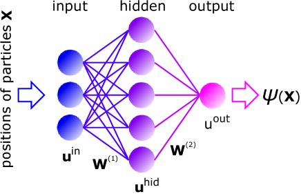
We use a feedforward artificial neural network, as illustrated in Fig. 1. The input units $u_{1}^{\rm in},u_{2}^{\rm in},\cdots,u_{N_{\rm in}}^{\rm in}$ are set to real numbers, where $N_{\rm in}$ is the number of input units. The value of each hidden unit is generated by all the input units through weights as

$$u_{i}^{\rm hid}=\sum_{j=1}^{N_{\rm in}}W_{ji}^{(1)}u_{j}^{\rm in}+b_{i}^{(1)},$$ (1)

where the weights $W_{ji}^{(1)}$ and biases $b_{i}^{(1)}$ are real numbers. In our feedforward network, there is only a single output, whose value is given by

$$u^{\rm out}=\sum_{i=1}^{N_{\rm hid}}W_{i}^{(2)}f(u_{i}^{\rm hid}),$$ (2)

where $N_{\rm hid}$ is the number of hidden units, the weights $W_{i}^{(2)}$ are real numbers, and $f$ is the activation function. In this paper, we adopt the hyperbolic tangent function, $f(x)=\tanh(x)$, as the activation function. We thus use a fully connected network with a single hidden layer. The number of parameters $W_{ji}^{(1)}$, $b_{i}^{(1)}$, and $W_{i}^{(2)}$ in this neural network is $(N_{\rm in}+2)N_{\rm hid}$.

We consider a system of $N$ identical bosons. Particle positions are written as $\bm{X}=(x_{1},x_{2},\cdots,x_{N})$ for one dimension and $\bm{X}=(\bm{x}_{1},\bm{x}_{2},\cdots,\bm{x}_{N})$ for higher dimensions. We input $\bm{\xi}(\bm{X})=(\xi_{1}(\bm{X}),\xi_{2}(\bm{X}),\cdots,\xi_{N_{\rm in}}(\bm{X}))$ into the neural network, where $\xi_{i}(\bm{X})$ are functions of the particle positions. The functions $\xi_{i}(\bm{X})$ are chosen to facilitate the representation of many-body states in the neural network, and depend on the problem, which will be specified later. The many-body wave function is given by the output unit as

$$\psi(\bm{X})=\exp(u^{\rm out}).$$ (3)

This wave function is not normalized. Our aim is to optimize the network parameters in such a way that if we input $\bm{\xi}(\bm{X})$ into the neural network, the output $\psi(\bm{X})=\exp(u^{\rm out})$ provides an approximate ground-state wave function. In other words, we use neural networks as variational wave functions. Since the ground-state wave functions of bosons can be taken to be positive everywhere, we only use a single output unit that gives a positive wave function $\psi(\bm{X})=\exp(u^{\rm out})$. If we use a network with two output units, complex-valued wave functions can be represented [10, 12].

The expectation value of a quantity $\hat{A}$ is calculated as follows. To deal with a large Hilbert space, we calculate the integration $\int d\bm{X}$ using the Monte Carlo method. Through Metropolis sampling, we obtain a series of samples $(\bm{X}_{1},\bm{X}_{2},\cdots,\bm{X}_{N_{\rm sample}})$, where the probability $P(\bm{X})$ of $\bm{X}$ being sampled is proportional to $\psi^{2}(\bm{X})$. Using these samples, the expectation value is calculated as

$$\langle\hat{A}\rangle = \frac{\int\psi(\bm{X})\hat{A}\psi(\bm{X})d\bm{X}}{\int\psi^{2}(\bm{X})d\bm{X}}$$ (4)

$$= \int P(\bm{X})\psi^{-1}(\bm{X})\hat{A}\psi(\bm{X})d\bm{X}$$

$$\simeq \frac{1}{N_{\rm sample}}\sum_{i=1}^{N_{\rm sample}}\psi^{-1}(\bm{X}_{i})\hat{A}\psi(\bm{X}_{i})$$

$$\equiv \langle\psi^{-1}\hat{A}\psi\rangle_{s}.$$

To minimize the energy $E$ of the system, we need to calculate the derivative of energy with respect to the network parameters as

$$\frac{\partial E}{\partial W} = \frac{\partial}{\partial W}\frac{\int\psi(\bm{X})\hat{H}\psi(\bm{X})d\bm{X}}{\int\psi^{2}(\bm{X})d\bm{X}}$$ (5)

$$\simeq 2\langle\psi^{-1}O_{W}\hat{H}\psi\rangle_{s}-2\langle\psi^{-1}\hat{H}\psi\rangle_{s}\langle O_{W}\rangle_{s},$$

where $W$ is one of the network parameters ($W_{ji}^{(1)}$, $b_{i}^{(1)}$, and $W_{i}^{(2)}$), $\hat{H}$ is the Hamiltonian of the system, and $O_{W}=\psi^{-1}\partial\psi/\partial W$. Using the gradient in Eq. (5), the network parameters are updated using the Adam scheme [27], by which energy converges faster than the steepest descent method [12]. Typically, $10^{4}$-$10^{5}$ updates are needed for energy convergence with $N_{\rm sample}\sim 10^{4}$ samples taken in each update.

It is important to choose initial values of the network parameters because if we use random numbers for this purpose and start the update procedure, the network state seriously fluctuates so that the calculation breaks down in most cases. This is different from previous cases focusing on lattice systems [10, 12], in which random numbers in the initial network parameters worked well. To prepare appropriate initial network parameters, we train the network so that it represents a wave function $\Psi_{\rm train}$. We train the network to maximize the overlap integral $K$ given by

$$K=\frac{\left[\int\Psi_{\rm train}(\bm{X})\psi(\bm{X})d\bm{X}\right]^{2}}{\int\Psi^{2}_{\rm train}(\bm{X})d\bm{X}\int\psi^{2}(\bm{X})d\bm{X}}\simeq\frac{\langle A\rangle_{s}^{2}}{\langle A^{2}\rangle_{s}},$$ (6)

where $A=\Psi_{\rm train}/\psi$. This is accomplished by using the gradient of $K$ with respect to network parameters as

$$\frac{\partial K}{\partial W}\simeq 2K\left(\frac{\langle AO_{W}\rangle_{s}}{\langle A\rangle_{s}}-\langle O_{W}\rangle_{s}\right).$$ (7)

Using the Adam scheme with Eq. (7), $K$ is maximized and $\psi$ converges toward $\Psi_{\rm train}$. The initial values of the network parameters in this training process can be random numbers with an appropriate magnitude [26]. For example, $\Psi_{\rm train}$ is chosen to be a noninteracting ground state, and the interaction is introduced adiabatically.

Figure 2: (Color online) Training of the neural network to represent the wave function in Eq. (8), where the overlap integral $K$ is given in Eq. (6). (a) Change in $K$ with respect to the number of network parameter updates for $N=5$ and 8. The number of hidden units is $N_{h}=20$. (b) $N_{h}$ dependence of $1-K$ after 20000 updates for $N=5$ and 8. The number of samples is $N_{\rm sample}=10^{4}$ for each update in (a) and (b), and $N_{\rm sample}=10^{6}$ to calculate the data points in (b).

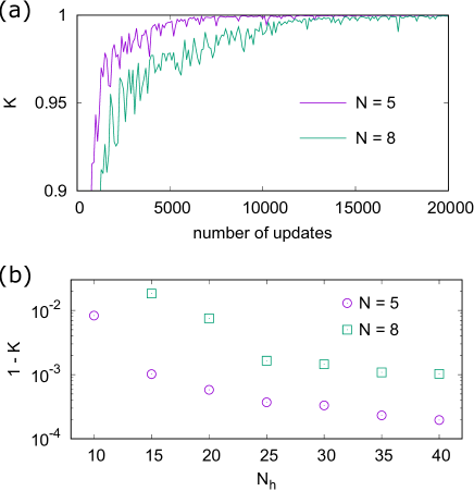
We demonstrate that the foregoing procedure increases $K$ and hence the wave function $\psi$ that is close to $\Psi_{\rm train}$ can be prepared. We take the target wave function as

$$\Psi_{\rm train}(\bm{X})=\prod_{i=1}^{N}e^{-x_{i}^{2}/2},$$ (8)

which is the ground state of $N$ bosons in a one-dimensional harmonic potential. The neural network inputs are simply the positions of the particles,

$$\bm{\xi}(\bm{X})=(x_{1},x_{2},\cdots,x_{N}),$$ (9)

and therefore, the number of input units is $N_{\rm in}=N$. Figure 2(a) shows how $K$ changes in the process of optimizing the network parameters. The value of $K$ approaches unity as the update steps proceed, and the wave function represented by the neural network approaches the target wave function $\Psi_{\rm train}$. The finally obtained overlap $K$ decreases with the number of atoms $N$, and increases with the number of hidden units $N_{h}$. Figure 2(b) shows the $N_{h}$ dependence of $1-K$ after 20000 updates, indicating that precision improves with an increase in $N_{h}$.

3 Results

3.1 Interacting bosons in one dimension

First, we apply our method to one-dimensional problems that have exact solutions to evaluate the precision of our proposed method. We consider the Calogero-Sutherland model [28, 29], in which bosons are confined in a harmonic potential and interact with each other through an inverse squared potential. The Hamiltonian for the system is given by

$$\hat{H}=\sum_{i=1}^{N}\left(-\frac{1}{2}\frac{\partial^{2}}{\partial x_{i}^{2}}+\frac{1}{2}x_{i}^{2}\right)+\sum_{j<k}\frac{\beta(\beta-1)}{(x_{j}-x_{k})^{2}},$$ (10)

where length and energy are normalized, and $\beta$ is an interaction parameter. The exact ground-state wave function for this Hamiltonian is available as [28]

$$\Psi_{\rm exact}=\exp\left(-\frac{1}{2}\sum_{i=1}^{N}x_{i}^{2}\right)\prod_{j<k}|x_{j}-x_{k}|^{\beta}$$ (11)

with the ground-state energy

$$E_{\rm exact}=\frac{N}{2}+\frac{\beta}{2}N(N-1).$$ (12)

The wave function in Eq. (11) satisfies the permutation symmetry of bosons.

We prepare the initial network parameters using the method in Sec. 2 with $\Psi_{\rm train}$ given in Eq. (8), which is the noninteracting ground state. The interaction potential is then gradually introduced as

$$\hat{H}_{\rm int}=\min\left[(an)^{2},\sum_{j<k}\frac{\beta(\beta-1)}{(x_{j}-x_{k})^{2}}\right],$$ (13)

where $n$ is the update step and $a$ determines the ramp speed of the potential. Initially $n=0$ and the interaction potential vanishes. As the update step $n$ increases, the peak of the interaction potential gradually rises. This prescription can avoid the calculation breaking down due to the sudden introduction of an infinite potential.

Figure 3: (Color online) Results for the Hamiltonian in Eq. (10) with $\beta=2$. (a) Wave function $\psi(x_{1},x_{2},x_{3}=0)$ for $N=3$. The middle and left panels are obtained with the input functions in Eqs. (9) and (14), respectively, and the right panel shows the exact solution in Eq. (11). (b) Energy convergence with respect to the number of network parameter updates for $N=5$ and 8. The number of hidden units is $N_{h}=20$. The interaction is gradually introduced as in Eq. (13) with $a=0.001$. The energies averaged over 100 updates are shown at intervals of 100 updates. (c) Energy and fidelity after 40000 updates. The error bars represent standard deviations for 5 runs. The number of samples is $N_{\rm sample}=10^{4}$ for each update in (a)-(c), and $N_{\rm sample}=10^{6}$ to calculate the data points in (c).

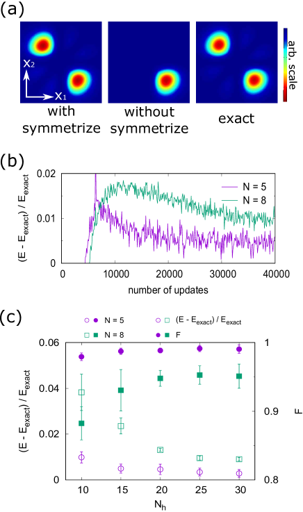
We first explore a simple input of particle positions as in Eq. (9); that is, the positions of the particles are directly input into the neural network. After a sufficient number of network update steps, we obtain the wave function, as shown in the middle panel of Fig. 3(a), which shows $\psi(x_{1},x_{2},0)$ for $N=3$. The permutation symmetry $x_{1}\leftrightarrow x_{2}$ is not satisfied in this wave function. This is because, in the Calogero-Sutherland model, many degenerate states exist near the ground states, such as a state satisfying $\psi(x_{1},x_{2},x_{3})=-\psi(x_{2},x_{1},x_{3})$. The linear combination of these states breaks the permutation symmetry, as shown in the middle panel of Fig. 3(a). To resolve this problem, we use as an input function

$$\bm{\xi}(\bm{X})=(x_{i_{1}},x_{i_{2}},\cdots,x_{i_{N}}),$$ (14)

where $x_{i_{1}}\leq x_{i_{2}}\leq\cdots\leq x_{i_{N}}$; that is, we input the sorted positions into the network. By this input method, bosonic permutation symmetry is maintained from the definition. The result of this input is shown in the leftmost panel of Fig. 3(a), which maintains the permutation symmetry, and accords with the exact solution shown in the rightmost panel of Fig. 3(a).

Figure 3(b) shows the evolution of energy with respect to update step [30]. Because of the gradual increase in interaction potential as in Eq. (13), the energy grows from $E<E_{\rm exact}$, and stochastically converges to the final value. Figure 3(c) shows the energy obtained after 40000 updates. The energy is improved as the number of hidden units $N_{h}$ is increased for $N_{h}=10$-20, since the representation ability of the network increases with $N_{h}$. However, the improvement saturates for $N_{h}\gtrsim 20$. Such saturation is also seen in Ref. Saito because network optimization becomes increasingly difficult for larger $N_{h}$. Figure 3(d) illustrates the fidelity $F$ of the wave function, defined as

$$F=\frac{\left[\int\Psi_{\rm exact}(\bm{X})\psi(\bm{X})d\bm{X}\right]^{2}}{\int\Psi^{2}_{\rm exact}(\bm{X})d\bm{X}\int\psi^{2}(\bm{X})d\bm{X}}\simeq\frac{\langle B\rangle_{s}^{2}}{\langle B^{2}\rangle_{s}},$$ (15)

where $B=\Psi_{\rm exact}/\psi$. The fidelity is larger than 0.99 for $N=5$ and larger than 0.95 for $N=8$. Fidelity improvement also saturates for $N_{h}\gtrsim 20$.

A periodic boundary condition can also be treated in our method. Specifically, we consider the Calogero-Sutherland model in free space with a periodic boundary condition. The Hamiltonian for the system is given by

$$\hat{H}=-\sum_{i=1}^{N}\frac{\partial^{2}}{\partial\theta_{i}^{2}}+\frac{\beta(\beta-1)}{2}\sum_{j<k}\frac{1}{\sin^{2}\frac{\theta_{j}-\theta_{k}}{2}},$$ (16)

where $0\leq\theta_{i}<2\pi$. The ground-state wave function and energy are obtained as [29]

$$\Psi_{\rm exact}=\prod_{j<k}\left(\sin\frac{\theta_{j}-\theta_{k}}{2}\right)^{\beta},$$ (17)

and

$$E_{\rm exact}=\frac{\beta^{2}}{12}N(N^{2}-1).$$ (18)

To incorporate the periodic boundary condition into the wave function produced by the neural network, we use an input method as follows. We first sort the positions as $\theta_{i_{1}}\leq\theta_{i_{2}}\leq\cdots\leq\theta_{i_{N}}$. If we directly input these positions into the network, a discontinuity arises at $\theta=0$, because the network does not know that $\theta=0=2\pi$. To avoid this problem, we take the distance between the adjacent positions, $\Delta_{1}\equiv\theta_{i_{2}}-\theta_{i_{1}}$, $\Delta_{2}\equiv\theta_{i_{3}}-\theta_{i_{2}}$, $\cdots,\Delta_{N}\equiv\theta_{i_{1}}+2\pi-\theta_{i_{N}}$. We also take their cyclic permutation. The input into the network is thus

$$\bm{\xi}(\bm{X})=(\Delta_{p},\Delta_{p+1},\cdots,\Delta_{N},\Delta_{1},\cdots,\Delta_{p-1}),$$ (19)

where $p$ is a random integer such that $1\leq p\leq N$.

Figure 4: (Color online) Results for the Hamiltonian in Eq. (16) with $\beta=2$. (a) Convergence of energy with respect to the number of network parameter updates for $N=5$ and 8. The number of hidden units is $N_{h}=20$. The interaction is gradually introduced as in Eq. (13) with $a=0.002$. The energies averaged over 100 updates are shown at intervals of 100 updates. (b) Energy and fidelity after 40000 updates. The error bars represent standard deviations for 5 runs. The number of samples is $N_{\rm sample}=10^{4}$ for each update in (a) and (b), and $N_{\rm sample}=10^{6}$ to calculate the data points in (b).

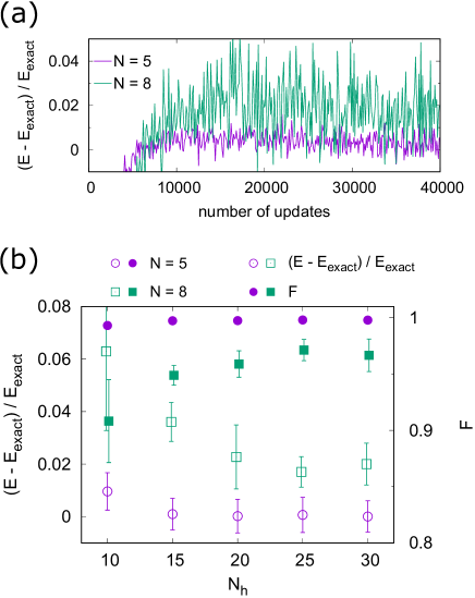
Figure 4(a) shows the change in energy with respect to the number of updates. As in the previous case, we gradually increase the interaction using Eq. (13), and the energy $E$ grows from $E<E_{\rm exact}$ and approaches $E_{\rm exact}$. Figure 4(b) shows the $N_{h}$ dependence of energy and fidelity. Also, in this case, results improve with an increase in $N_{h}$ for $N_{h}\lesssim 20$ and saturate for $N_{h}\gtrsim 20$. The fidelity is larger than 0.99 for $N=5$ and larger than 0.95 for $N=8$.

3.2 Few-body bound states in three dimensions

We consider bosons in three-dimensional space with an attractive interaction between particles. As an interesting demonstration of such quantum many-body problems, we aim to produce the Efimov bound state, which is a three-body bound state near the resonant interaction [31, 32]. The Hamiltonian for the system is assumed to be

$$\hat{H}=\sum_{i=1}^{N}\left(-\frac{1}{2}\frac{\partial^{2}}{\partial\bm{x}_{i}^{2}}+\frac{\alpha}{2}\bm{x}_{i}^{2}\right)-\sum_{j<k}\frac{V_{0}}{2r_{0}^{2}}\exp\left[-\frac{(\bm{x}_{j}-\bm{x}_{k})^{2}}{2r_{0}^{2}}\right],$$ (20)

where $\bm{x}_{i}$ are three-dimensional vectors of the position of the $i$th particle, $\alpha$ is the strength of harmonic confinement, and $V_{0}$ and $r_{0}$ are the strength and range of the Gaussian interaction, respectively. The parameter $\alpha$ is controlled to promote bound-state formation. We assume that interaction strength is at the first resonance, $V_{0}\simeq 2.684$, at which the first two-body bound state emerges at this interaction strength.

The Jacobi coordinate is convenient to remove the translational degree of freedom. We define the Jacobi coordinate $\bm{r}_{i}$ as

$$\bm{r}_{N-j+1}=\sqrt{\frac{2j}{j+1}}\left[\bm{x}_{j+1}-\frac{1}{j}\left(\bm{x}_{1}+\bm{x}_{2}+\cdots+\bm{x}_{j}\right)\right]$$ (21)

for $j=1,2,\cdots,N-1$, and

$$\bm{r}_{1}=-\sqrt{\frac{2}{j(j+1)}}\left(\bm{x}_{1}+\bm{x}_{2}+\cdots+\bm{x}_{N}\right).$$ (22)

Using this Jacobi coordinate, the Hamiltonian can be divided into $\hat{H}=\hat{H}_{1}+\hat{H}^{\prime}$ with

$$\hat{H}_{1} = -\frac{1}{N+1}\frac{\partial^{2}}{\partial\bm{r}_{1}^{2}}+\frac{N+1}{4}\alpha\bm{r}_{1}^{2},$$ (23)

$$\hat{H}^{\prime} = \sum_{i=2}^{N}\left(-\frac{\partial^{2}}{\partial\bm{r}_{i}^{2}}+\frac{\alpha}{4}\bm{r}_{i}^{2}\right)-\sum_{j<k}\frac{V_{0}}{2r_{0}^{2}}\exp\left[-\frac{(\bm{x}_{j}-\bm{x}_{k})^{2}}{2r_{0}^{2}}\right].$$

Since the Gaussian interaction term in $\hat{H}^{\prime}$ does not include $\bm{r}_{1}$, the ground-state wave function can be written as

$$\psi(\bm{x}_{1},\bm{x}_{2},\cdots,\bm{x}_{N})=e^{-\frac{N+1}{4}\alpha^{1/2}r_{1}^{2}}\psi^{\prime}(\bm{r}_{2},\cdots,\bm{r}_{N}),$$ (25)

where $\psi^{\prime}$ is the ground state for $\hat{H}^{\prime}$. Thus, we seek the wave function $\psi^{\prime}$ that minimizes $E^{\prime}=\langle\hat{H}^{\prime}\rangle$. Metropolis sampling is performed in the coordinate $\bm{X}$; i.e., we sample $\bm{x}_{1}$, $\bm{x}_{2}$, $\cdots$, $\bm{x}_{N}$ (not $\bm{r}_{2},\cdots,\bm{r}_{N}$) in each sampling with a probability $\psi^{2}=e^{-\frac{N+1}{2}\alpha^{1/2}r_{1}^{2}}\psi^{{}^{\prime}2}$ in Eq. (25), where the network gives $\psi^{\prime}=\exp(u^{\rm out})$.

We prepare the initial state of the network parameters using

$$\Psi_{\rm train}=\prod_{i=2}^{N}e^{-\alpha^{1/2}r_{i}^{2}/4},$$ (26)

which is the noninteracting ground state. The interaction is then gradually introduced as

$$V_{0}=2.684\min\left(n/n_{0},1\right),$$ (27)

where $n$ is the number of update steps and we take $n_{0}=5000$. Increasing the interaction gradually avoids sudden change in network parameters which could cause the calculation to break down.

Figure 5: (Color online) Three-dimensional bound states for the Hamiltonian in Eq. (3.2). (a) Changes in $E^{\prime}$ and the degree of permutation symmetry $P$ with respect to the number of network parameter updates, where $P$ is defined in Eq. (31). The inset shows the hyperradial distribution $D(R)$ after 40000 updates. (b) Energies of bound states for $N=3$-10 after 40000 updates of the network parameters (circles). The number of hidden units is $N_{h}=30$ for $N\leq 7$ and $N_{h}=60$ for $N\geq 8$. The squares indicate energies $E_{\rm ref}$ taken from Ref. Yan. The inset shows $(E^{\prime}-E_{\rm ref})/|E_{\rm ref}|$. The error bars represent standard deviations for 5 runs. The number of samples is $N_{\rm sample}=10^{4}$ for each update in (a) and (b), and $N_{\rm sample}=10^{6}$ to calculate the data points in (b).

First, we consider the case of $N=3$. The simplest input into the network is

$$\bm{\xi}(\bm{X})=(r_{2}^{(x)},r_{2}^{(y)},r_{2}^{(z)},r_{3}^{(x)},r_{3}^{(y)},r_{3}^{(z)}),$$ (28)

where $r_{i}^{(x)}$, $r_{i}^{(y)}$, and $r_{i}^{(z)}$ are $x,y$, and $z$ components of the Jacobi vector. However, the input function in Eq. (28) was found to be inappropriate. The calculation is unstable in many cases, and even if stability is maintained, convergence is very slow. This is partly because rotational degrees of freedom remain in the coordinates in Eq. (28). We then examine the input function as

$$\bm{\xi}(\bm{X})=(\Delta_{12},\Delta_{13},\Delta_{23}),$$ (29)

where

$$\bm{\Delta}_{12} = \bm{x}_{1}-\bm{x}_{2}=-\bm{r}_{3},$$

$$\bm{\Delta}_{13} = \bm{x}_{1}-\bm{x}_{3}=-\frac{1}{2}(\sqrt{3}\bm{r}_{2}+\bm{r}_{3}),$$

$$\bm{\Delta}_{23} = \bm{x}_{2}-\bm{x}_{3}=-\frac{1}{2}(\sqrt{3}\bm{r}_{2}-\bm{r}_{3}).$$ (30)

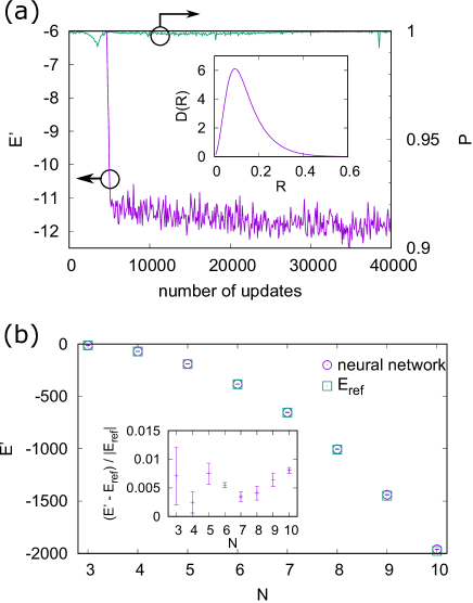
In this input method, the distances between particles are input into the neural network; this takes into account not only translational symmetry but also rotational symmetry. Figure 5(a) shows the change in energy with respect to update steps. The energy drops to $E\simeq-12$, which indicates that the bound state is formed. The energy is close to $-11.9$ obtained in Ref. Yan. To promote formation of the bound state, we set $\alpha=1.5$ until 10000 updates, and $\alpha=1$ subsequently. The inset in Fig. 5(a) shows the hyperradial distribution $D(R)$ of the state after convergence, where the hyperradius $R$ is defined as $R^{2}=(\Delta_{12}^{2}+\Delta_{13}^{2}+\Delta_{23}^{2})/3$. The particles are localized in $R\ll 1$, and hence the harmonic potential in Eq. (3.2) is almost irrelevant for the binding. In fact, a very similar result is obtained when the harmonic potential is removed ($\alpha=0$) after the bound state is formed. It was also confirmed that the bound state is “Borromean”, i.e., the bound state is formed for $V_{0}<2.684$ for which the two-body bound state does not exist.

In our method with the input function in Eq. (29), the bosonic permutation symmetry of the particles is not imposed explicitly. To confirm that the obtained wave function exhibits permutation symmetry, we introduce the overlap integral given by

$$P = \frac{2}{N(N+1)}\sum_{j<k}\frac{\left[\int\psi(\hat{P}_{jk}\bm{X})\psi(\bm{X})d\bm{X}\right]^{2}}{\int\psi^{2}(\hat{P}_{jk}\bm{X})d\bm{X}\int\psi^{2}(\bm{X})d\bm{X}}$$ (31)

$$\simeq \frac{2}{N(N+1)}\sum_{j<k}\frac{\langle A_{jk}\rangle_{s}^{2}}{\langle A_{jk}^{2}\rangle_{s}},$$

where $\hat{P}_{jk}$ exchanges the positions of the $j$th and $k$th particles, and $A_{jk}=\psi(\hat{P}_{jk}\bm{X})/\psi(\bm{X})$. If the wave function exhibits permutation symmetry, $P$ becomes unity. From Fig. 5(a), we find that the obtained wave function indeed acquires permutation symmetry.

Figure 5(b) shows the energies for $N\geq 3$. The input function is

$$\bm{\xi}(\bm{X})=(\Delta_{12},\Delta_{13},\cdots,\Delta_{1N},\Delta_{23},\Delta_{24},\cdots,\Delta_{N-1,N}),$$ (32)

and the number of input units is $N(N-1)/2$. For comparison, the energies $E_{\rm ref}$ obtained in Ref. Yan are shown, in which the path-integral Monte Carlo method is used. The energies obtained by the present method are in reasonable agreement with those obtained by the pre-existing method. At present, our method cannot surpass the precision of the path-integral Monte Carlo method. However, in our method, wave functions are obtained directly, which facilitates the study of quantum few-body problems.

4 Conclusions

We have developed a method to obtain approximate ground-state wave functions of quantum few-body problems using artificial neural networks. Bosons in continuous space were considered and particle positions or their functions were input into neural networks, which were optimized to output the desired wave functions. The method was applied to the Calogero-Sutherland model in one-dimensional space and the results were compared with exact solutions. Using the appropriate input functions in Eqs. (14) and (19), the bosonic permutation symmetry of the wave functions was taken into account, and we successfully obtained the approximate ground-state wave functions. The method was also applied to the three-dimensional problem of bound states with resonant interaction. The Efimov trimer was obtained and its energy was close to that calculated in the previous study. Also, in this case, the appropriate input function in Eq. (29) was important to efficiently reach the ground state. The bound states for $N>3$ bosons were also obtained.

In the present paper, we have restricted our attention to a fully connected neural network with a single hidden layer. Deep neural networks with multiple hidden layers have larger representation power, and one may posit that the use of such networks would improve the results. However, network optimization becomes difficult as the complexity of the network structure increases. In fact, we observed that the precision of results saturates as the number of hidden units $N_{h}$ increases, even for the single hidden layer. It is important to find a more efficient network structure and input method to facilitate optimization of the network parameters. We also need to find an appropriate way to deal with fermions.