Article Summary — followed by the full article on p. 4
Small vulnerable sets determine large network cascades
in power grids
Yang Yang,¹ Takashi Nishikawa,^1,2,∗ Adilson E. Motter^1,2
Science 358, eaan3184 (2017),    DOI: 10.1126/science.aan3184
Animated summary: http://youtu.be/c9n0vQuS2O4
¹Department of Physics and Astronomy, Northwestern University, Evanston, IL 60208, USA
²Northwestern Institute on Complex Systems, Northwestern University, Evanston, IL 60208, USA
^∗Corresponding author. E-mail: t-nishikawa@northwestern.edu

Cascading failures in power grids are inherently network processes, inwhich an initially small perturbation leads to a sequence of failures that spread through the connections between system components. An unresolved problem in preventing major blackouts has been to distinguish disturbances that cause large cascades from seemingly identical ones that have only mild effects. Modeling and analyzing such processes are challenging when the system is large and its operating condition varies widely across different years, seasons, and power demand levels.

Multicondition analysis of cascade vulnerability is needed to answer several key questions: Under what conditions would an initial disturbance remain localized rather than cascade through the network? Which network components are most vulnerable to failures across various conditions? What is the role of the network structure in determining component vulnerability and cascade sizes? To address these questions and differentiate cascading-causing disturbances, we formulated an electrical-circuit network representation of the U.S.-South Canada power grid—a large-scale network with more than 100,000 transmission lines—for a wide range of operating conditions. We simulated cascades in this system by means of a dynamical model that accounts for transmission line failures due to overloads and the resulting power flow reconfigurations.

Summary Figure: Cascade-resistant portion of the U.S.-South Canada power grid. The network is visualized on a cartogram that equalizes the density of nodes. (Top) Power lines that never underwent outage in our simulations under any grid condition are shown in green, whereas all the other lines—whose vulnerability varies widely—are in gray. (Bottom) Spreading of a cascade triggered by three failures at time $t=0$ (arrows), which resulted in $254$ failures at $t=100$ (the end of the cascade in linearly rescaled time).

To quantify cascade vulnerability, we estimated the probability that each transmission line fails in a cascade. Aggregating the results from multiple conditions into a single network representation, we created a systemwide vulnerability map, which exhibits relatively homogeneous geographical distribution of power outages but highly heterogeneous distribution of the underlying overload failures. Topological analysis of the network representation revealed that the transmission lines vulnerable to overload failures tend to occupy the network’s core, characterized by links between highly connected nodes. We found that only a small fraction of the transmission lines in the network (well below 1% on average) are vulnerable under a given condition. When measured in terms of node-to-node distance and geographical distance, individual cascades often propagate far from the triggering failures, but the set of lines vulnerable to these cascades tend to be limited to the region in which the cascades are triggered. Moreover, large cascades are disproportionately more likely to be triggered by initial failures close to the vulnerable set.

Our results imply that the same disturbance in a given power grid can lead to disparate outcomes under different conditions—ranging from no damage to a large-scale cascade. The association between large cascades and the triggering failures’ proximity to the vulnerable set indicates that the topological and geographical properties of the vulnerable set is a major factor determining whether the failures spread widely. Because the vulnerable set is small, failures would often repeat on the same lines in the absence of interventions. Although the power grid represents a complex system in which changes can have unanticipated effects, our analysis suggests failure-based allocation of resources as a strategy in upgrading the system for improved resilience against large cascades.

Small vulnerable sets determine large network cascades in power grids

One Sentence Summary: Computational analysis reveals that cascades in power grids are driven by the recurrent failure of few—but central—components.

The understanding of cascading failures in complex systems has been hindered by the lack of realistic large-scale modeling and analysis that can account for variable system conditions. Here, using the North American power grid, we identify, quantify, and analyze the set of network components that are vulnerable to cascading failures under any out of multiple conditions. We show that the vulnerable set consists of a small but topologically central portion of the network and that large cascades are disproportionately more likely to be triggered by initial failures close to this set. These results elucidate aspects of the origins and causes of cascading failures relevant for grid design and operation, and demonstrate vulnerability analysis methods that are applicable to a wider class of cascade-prone networks.

Cascading failures are inherently large-scale network processes that cannot be satisfactorily understood from a local or small-scale perspective. In blackouts caused by cascading failures in the power grid, a relatively small local disturbance triggers a sequence of grid component failures, causing potentially large portions of the network to become inactive with costly outcomes. In the North American power grid  (?), for instance, a single widespread power outage can inflict tens of billions of dollars in losses  (?), and smaller but more frequent outages can amount to a yearly combined impact comparable to that of the largest blackouts  (?). Yet, not much is known about what distinguishes disturbances that cause cascades from seemingly identical ones that do not. Despite the significant advances made through conceptual modeling of general cascades  (?, ?, ?, ?, ?, ?, ?) and physics-based modeling of power-grid–specific cascades  (?, ?, ?, ?), a major obstacle still remains: the lack of realistic large-scale models and a framework for analyzing cascade vulnerability under variable system conditions. Developing such a framework is challenging for three reasons: (i) detailed data combining both structural and dynamical parameters are scarce, (ii) the system condition varies on a wide range of time scales, and (iii) computational resources required for modeling grow combinatorially with system size  (?). These challenges have limited the applicability of most previous studies to vulnerability under a single condition and either to smaller scales than those required to describe large cascades or to models that are not constrained by real data. Similar hurdles exist in studying large-scale failures in the broader context of complex networks  (?, ?, ?), including extinction cascades in ecological systems  (?, ?, ?) and contagion dynamics in financial systems  (?, ?).

Here we focus on the U.S.-South Canada power grid, which is the largest contiguous power grid amenable to modeling. This system is composed of three interconnections (Texas, Western, and Eastern; Fig. 1A), which are separate networks of alternating current generators and power consumers connected by transmission lines (network components are illustrated in Fig. 1B). To study this system, we used the data reported in the Federal Energy Regulatory Commission (FERC) Form 715. For each interconnection, the data represent various snapshots of the system, spanning the years 2008–2013 and covering multiple seasons as well as both on- and off-peak demand levels, which correspond to different operating conditions. Basic properties of the $46$ snapshots we used are listed in Table S1. A representation of each snapshot was constructed by processing the parameters of individual power-grid components, including power generation and demand as well as the capacity of transmission lines. Central to the analysis of cascade vulnerability in this system is that our approach distinguishes (i) transmission lines (or simply lines) that do not carry flow because they have become out of service due to protective relay actions, equipment malfunctions, operational errors, or physical damages (primary failures); and (ii) lines that do not carry flow at the end of the cascades because they are de-electrified due to the outage of other lines (secondary failures).

Geographic layout of vulnerabilities

The vulnerability of a given transmission line $\ell$ can be quantified by the probability $p_{\ell}$ that the line fails in a cascade event triggered by a random perturbation to a given snapshot of a given interconnection. To estimate $p_{\ell}$, we used a cascade dynamics model that combines key elements from previous models  (?, ?, ?) to suitably account for the physics of cascading failures. In this model, the initial state of the system for the given snapshot is determined by computing the power flow over all transmission lines and transformers from the power flow equation (see Materials and Methods, Supplementary Materials). The triggering perturbation was implemented through the removal of a set of $n_{\text{t}}$ lines, representing line outages due to unforeseen events, such as damage to power lines caused by extreme weather and unplanned line shutdowns caused by operational errors. After this initial removal, a cascade event was modeled as an iterative process, with each step consisting of a single power line outage due to overheating (primary failure), followed by the redistribution of power flow in the network to compensate for the lost flow over the failed line. Line overheating is modeled by a temperature evolution equation  (?), and flow redistribution is determined by solving the power flow equation again; if a primary line failure disconnects the network into multiple parts with unbalanced supply and demand, the power generation and consumption in each part are adjusted (similarly to how generation reserves and power shedding are used in grid operation) to allow for the subsequent power flow calculation. The failure probability $p_{\ell}$ was estimated from $K$ such simulated cascade events, including those with no subsequent failures. Further details on the triggering perturbations and cascade dynamics model can be found in Materials and Methods, Supplementary Materials.

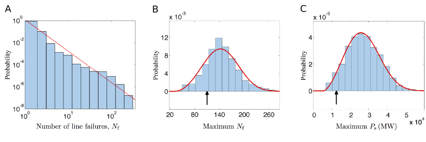
Fig. S1: Validation of the cascade model against historical data for the Western interconnection. The cascade size from simulations and from real events are compared by the number of (primary) line failures $N_{\text{f}}$ for the BPA data comprised of a total of $5{,}227$ cascades, and by the amount of power shed $P_{\text{s}}$ for the NERC data comprised of $93$ large cascades ($\geq\!300$MW). (A) Histogram of the cascade size ($N_{\text{f}}$) from simulations in which the number of triggering line failures follows the empirical distribution derived from the BPA data. The simulation results are in agreement with the linear regression (dashed line) of the BPA data compiled in Ref. (45). (B) Histogram of the largest cascade size in a set of $5{,}227$ samples of $N_{\text{f}}$ drawn from the probability distribution of cascade size computed from the simulations, for $5{,}000$ independent realizations of this set (blue). Due to the rareness of large cascade events and the corresponding under-sampling in simulations, we used the kernel density estimation [for a Gaussian kernel with its width chosen according to the Silverman’s rule of thumb (48)] to approximate the $0.1\%$ tail of the distribution. The $p$-value of the largest $N_{\text{f}}$ from the BPA historical data (black arrow) was found to be $0.42$ under the hypothesis that the observed largest $N_{\text{f}}$ follows the generalized extreme value distribution (49) fitted to the histogram (red curve). (C) Same as (B) but for $P_{\text{s}}$, using sets of $93$ samples drawn from the probability distribution computed from simulations, considering only the large simulated cascades. Each maximum $P_{\text{s}}$ was adjusted by a factor $(0.98)^{y}$ to incorporate approximately $2\%$ annual increase of the power demand, where $y$ is an integer randomly chosen from $2$ to $14$ to trace back from the year of the simulated data (2008) to years of historical data ($1984$–$2006$). We found the $p$-value of the largest $P_{\text{s}}$ from the NERC historical data (black arrow) to be $0.07$ under the hypothesis that the observed largest $P_{\text{s}}$ follows the generalized extreme value distribution fitted to the histogram (red curve). In both (B) and (C), we cannot reject the null hypothesis that the real largest cascade size follows the fitted distribution at a significance level of $5\%$.

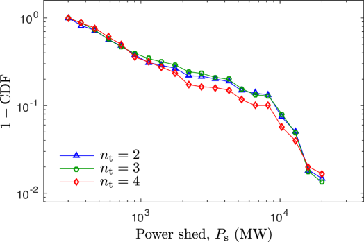
Fig. S2: Robustness of cascade size distribution with respect to the number of triggering line failures. Cumulative distribution functions (CDF) of the cascade size $P_{\text{s}}$ for large simulated cascades ($\geq\!300$MW) triggered by disabling $n_{\text{t}}=2$ (blue), $n_{\text{t}}=3$ (green), and $n_{\text{t}}=4$ (red) power lines in the Western interconnection. For each $n_{\text{t}}$, the CDF was calculated by combining the estimated distribution of $P_{\text{s}}$ for all snapshots using the weights given in Table S1. The Kolmogorov-Smirnov test (47) cannot reject the hypothesis that the size of cascades triggered by $n_{\text{t}}=3$ line failures has the same underlying distribution as of those triggered by $4$ line failures ($p$-value = $0.22$) or $2$ line failures ($p$-value = $0.08$). This supports the conclusion that the distribution does not depend sensitively on the size of the perturbation, even though the size of the largest cascade might.

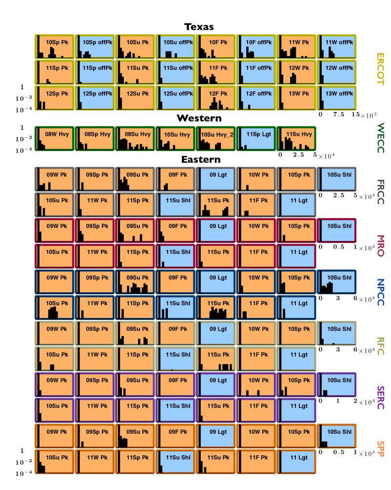
Fig. S3: Distribution of cascade size from simulated events broken down by region and snapshot. Histograms of the relative frequencies of cascade size $P_{\text{s}}$ (measured in MW) for events triggered in different NERC regions (marked by the color of the box border), where each panel represents a different snapshot of the power grid for the given region. The acronyms for the snapshots and the abbreviations for the triggering regions are defined in Tables S1 and S2, respectively. The distributions have the same horizontal linear scale within each region and the same vertical logarithmic scale for all regions. The background color indicates the level of power demand for each snapshot, with orange for high demand and blue for moderate and low demand.

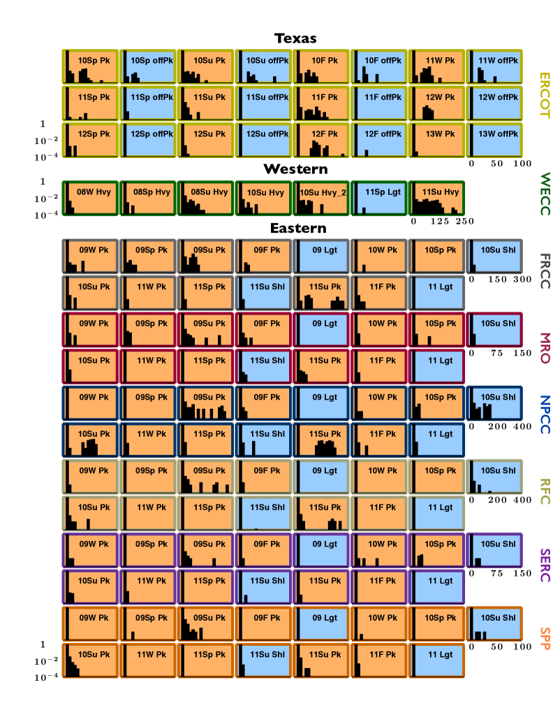
Fig. S4: Same as Fig. S3 but now for cascade size measured by the number of (primary) line failures, $\boldsymbol{N_{\text{f}}}$.

We validated the model against historical line outage data available from the Bonneville Power Administration (BPA) with respect to the distribution of cascade sizes measured by the number of (primary) line failures $N_{\text{f}}$ (Materials and Methods, Supplementary Materials, and Fig. S1A). We also validated the extremal cascade size measured by $N_{\text{f}}$ and power shed $P_{\text{s}}$ (defined as the reduction in the amount of power delivered to the consumers) against the BPA data and grid disturbance data from the North American Electric Reliability Corporation (NERC), respectively (Materials and Methods, Supplementary Materials, and Fig. S1, B and C). All simulations were performed with $n_{\text{t}}=3$, as the cascade size distribution for a given snapshot did not differ significantly for other choices of $n_{\text{t}}$ (Fig. S2). However, the distribution exhibited considerable variation across different snapshots, both when cascade size was measured by the power shed $P_{\text{s}}$ (Fig. S3), and when measured by the number of line failures $N_{\text{f}}$ (Fig. S4).

To aggregate results over different snapshots, we used a node to represent the set of all buses associated with the same geographic location across all snapshots in our dataset, where the term bus refers to a connection point between components of a power grid, such as transmission lines, transformers, and generators (Fig. 1B). This definition of a node typically corresponds to a substation and can include generators at a nearby power plant and/or an electrical load representing local power consumption. We used a link between a pair of nodes to represent the set of all (parallel) transmission lines directly connecting the same pair of nodes in at least one snapshot, where each of these transmission lines connects two different buses (one from each node in the pair). In this network, the aggregated vulnerability $p_{l}:=\langle p_{\ell}\rangle$ of a link $l$, which we refer to as the a-vulnerability, is a weighted average of the failure probabilities over the lines represented by the link $l$ and over the various snapshots:

$$\langle p_{\ell}\rangle=\frac{\sum_{c}\sum_{\ell}p_{\ell;c}w_{c}}{\sum_{c}\sum_{\ell}w_{c}},$$ (1)

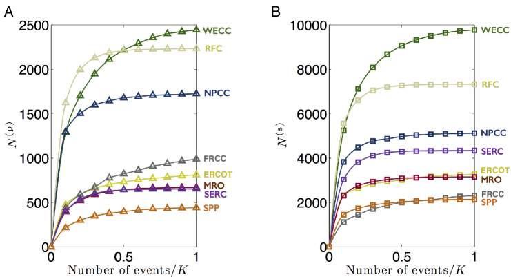
Fig. S5: Dependence of the number of failing links on the number of simulated events. (A and B) Number of links $N^{\text{(p)}}$ that experience primary failures (A) and number of links $N^{\text{(s)}}$ that experience secondary failures (B) versus the (normalized) number of simulated events sampled randomly from all $K$ events. Each symbol is colored by the region of the triggering line failures and represents an average over $100$ independent samples. Both $N^{\text{(p)}}$ and $N^{\text{(s)}}$ grow increasingly slower and appear to saturate as the sample size increases, justifying our choices of $K$ given in Table S1.

where $c$ indexes the different snapshot conditions simulated, and the sum over $\ell$ is limited to the set of transmission lines defining the link $l$ for the given $c$. Here, $p_{\ell;c}$ is the probability of line failure in the simulated perturbations of the system (the values of $K$ we used are given in Table S1 and justified in Fig. S5) and $w_{c}$ represents the weight assigned to each snapshot (Table S1). In our analyses, we present the a-vulnerability separately for primary failures $\bigl{(}$denoted by $\langle p^{\text{(p)}}_{\ell}\rangle\bigr{)}$, secondary failures $\bigl{(}$denoted by $\langle p^{\text{(s)}}_{\ell}\rangle\bigr{)}$, and the combination of both primary and secondary failures (denoted by $\langle p_{\ell}\rangle$ itself).

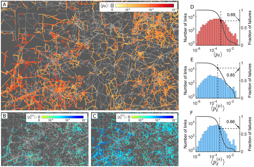
Figure 2: Vulnerability map of the U.S.-South Canada power grid. (A) Averaged failure probability of transmission lines, including primary and secondary failures, expressed as the total a-vulnerability of links $\langle p_{\ell}\rangle$. Since the structure of the power grid varies slightly from one snapshot to another, we visualize the a-vulnerability using a single network constructed to represent all snapshots of each interconnection by regarding the set of all buses at a given geographical location as a node and all transmission lines connecting two nodes as a single link. Each link is color-coded by the failure probability $\langle p_{\ell}\rangle$ estimated as a weighted average over all lines in all snapshots, where gray indicates links whose estimated probability is zero. (B and C) Same as in (A), but color-coded separately for the a-vulnerability to primary failures $\langle p^{\text{(p)}}_{\ell}\rangle$ (B) and the a-vulnerability to secondary failures $\langle p^{\text{(s)}}_{\ell}\rangle$ (C). Panels (A), (B), and (C) correspond to the same unidentified portion of the U.S.-South Canada map. (D) Histogram of the a-vulnerability $p_{l}=\langle p_{\ell}\rangle$ and the curve for $f(p):=\sum^{\prime}p_{l}/\sum_{l}p_{l}$, where $\sum^{\prime}$ denotes the sum over all links $l$ satisfying $p_{l}\geq p$. The function $f(p)$ thus represents the fraction of all failures that are associated with links of a-vulnerability $p$ or larger. (E and F) Same as in (D), but with $\langle p_{\ell}\rangle$ replaced by $\langle p^{\text{(p)}}_{\ell}\rangle$ and $\langle p^{\text{(s)}}_{\ell}\rangle$, respectively. In each of the panels (D), (E), and (F), the vertical and horizontal dashed lines indicate, respectively, the minimum a-vulnerability $p^{*}$ among the most vulnerable $20$% of all failing links and the fraction $f(p^{*})$ of failures accounted for by these links.

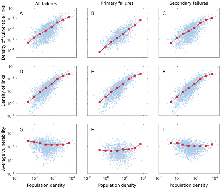
Fig. S6: Correlation between link vulnerability and population density. (A) Density of links with nonzero a-vulnerability $\langle p^{\text{\color[rgb]{1,1,1}p}}_{\ell}\rangle$ in the contiguous U.S. as a function of population density. For each county, the population density (in km^-2) was determined from the 2010 census data and the geographic coordinates of the county’s boundaries. The density of vulnerable links for a county was computed by counting the number of links with $\langle p^{\text{\color[rgb]{1,1,1}p}}_{\ell}\rangle>0$ that are connected to nodes within its boundaries, divided by the area of the county (in km²). The blue scatter points correspond to individual counties, whereas the red curve indicates the average over multiple counties computed by logarithmic binning with respect to population density. (B and C) The same as in (A) but shown separately for the vulnerability to primary failures $\langle p^{\text{(p)}}_{\ell}\rangle$ (B) and the vulnerability to secondary failures $\langle p^{\text{(s)}}_{\ell}\rangle$ (C). (D to F) Density of all links (vulnerable or not) as a function of population density, showing positive correlation similar to that observed in (A to C). (G to I) Average a-vulnerability (over all links connected to nodes in a given county) as a function of population density, showing no clear correlation.

We constructed the a-vulnerability map of the U.S.-South Canada power grid (shown in Fig. 2, A to C, for a portion of the grid). Over the entire network, we found that only $10.8\%$ of all links ever underwent a primary failure in our simulations and that secondary failures were on average $3.77$ times more prevalent than primary ones (Table S3). We also found that a-vulnerability was very unevenly distributed among the links, with 20% of the failing links (which in the case of primary failures correspond to only 2.16% of all links) accounting for about 85%, 66%, and 69% of the primary failures, secondary failures, and combined set of all failures, respectively (Fig. 2, D to F). Also uneven was the geographical distribution of links with nonzero a-vulnerability (Fig. 2, A to C), whose density was correlated positively with population density. This correlation was mainly due to the bias toward higher density of links in more densely populated areas, as it disappeared when a-vulnerability was averaged over the links in each geographical area to control for this bias. However, substantial geographical heterogeneity still remained for the averaged a-vulnerability, ranging over several orders of magnitude when calculated for individual U.S. counties. These observations were validated with the U.S. county population data from the 2010 census and the geographic coordinates of county boundaries (Fig. S6). Among the $48$ states and the District of Columbia represented in the U.S. portion of the network, the three least vulnerable ones were West Virginia (average $\langle p_{\ell}\rangle$ of $3.2\times 10^{-5}$), Tennessee (average $\langle p_{\ell}\rangle$ of $3.5\times 10^{-5}$), and Mississippi (average $\langle p_{\ell}\rangle$ of $3.8\times 10^{-5}$), all in the middle third of the population density ranking. However, some states among the least vulnerable did have relatively high or low population density, such as Illinois and Nebraska, which ranked $13$th and $43$rd in population density while having the $5$th and $6$th lowest a-vulnerability, respectively. The heterogeneity of a-vulnerability is visualized in Fig. 3A with a map representation that equalizes the density of nodes. The breakdown of this representation into primary and secondary failures, presented in Fig. 3, B and C, shows that a-vulnerability to primary failures was more heterogeneously distributed than a-vulnerability to secondary failures. Over all pixels with nonzero a-vulnerability, the standard deviation of $\log\,\langle\overline{p^{\phantom{\text{p}}}_{\ell}}\rangle$ was $0.48$ ($89.2\%$), of $\log\,\langle\overline{p^{\text{(p)}}_{\ell}}\rangle$ was $0.58$ ($57.5\%$) and of $\log\,\langle\overline{p^{\text{(s)}}_{\ell}}\rangle$ was $0.41$ ($87.0\%$), where the number in parenthesis represents the fraction of such pixels. The homogeneity in the distribution of secondary failures, which were several times more numerous than primary failures, underlies the relatively homogeneous aggregated distribution of the resulting power outages observed in Fig. 3A.

Network characterization of vulnerabilites

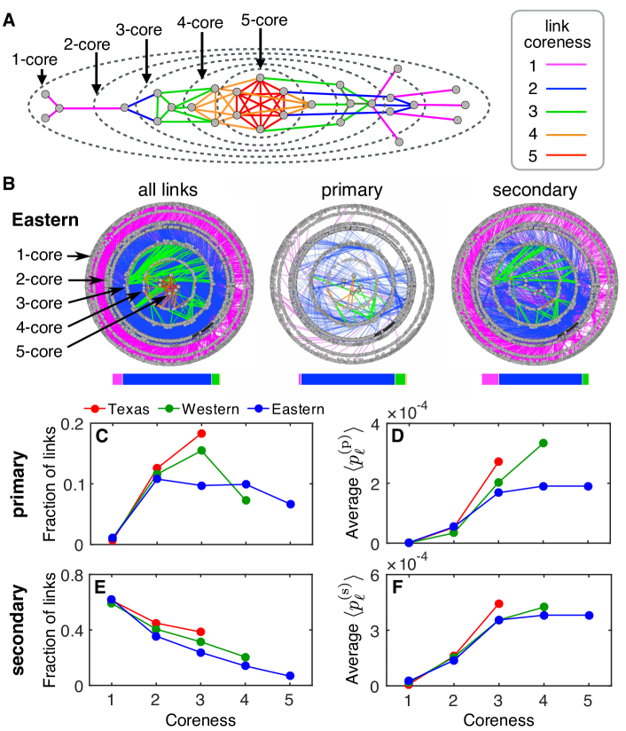
Figure 4: Characterization of vulnerability through $k$-core decomposition. (A) Coreness-based network visualization, where nodes with higher coreness are placed closer to the center. (B) Visualization of the $k$-core decomposition of the Eastern interconnection, showing (left) all the links in the network, (middle) only the links with nonzero a-vulnerability to primary failures $\bigl{(}\langle p^{\text{(p)}}_{\ell}\rangle>0\bigr{)}$, and (right) only the links with nonzero a-vulnerability to secondary failures $\bigl{(}\langle p^{\text{(s)}}_{\ell}\rangle>0\bigr{)}$. The bar under each panel shows the distribution of link coreness, color-coded as in (A). (C) Fraction of links with $\langle p^{\text{(p)}}_{\ell}\rangle>0$ among all links of a given coreness. (D) Average of $\langle p^{\text{(p)}}_{\ell}\rangle$ over all links of a given coreness with $\langle p^{\text{(p)}}_{\ell}\rangle>0$. (E and F) Counterparts of (C) and (D) for secondary failures.

Our characterization of a-vulnerability allows us to study how the observed cascade dynamics depend on the network structure and to identify the topological centrality of individual links as a determinant. Topological centrality can be quantified through the concept of $k$-core  (?, ?, ?, ?), which is defined as the largest subnetwork in which every node has at least $k$ links (that is, it has degree $k$). The $k$-core of a given network can be obtained by recursively removing all nodes with degree $<k$ until all nodes in the remaining network have degree $\geq k$. Repeating this for $k=1,2,\ldots$ determines the $k$-core decomposition of the network. The coreness of a node is then defined as the (unique) integer $c$ for which this node belongs to the $c$-core but not to the $(c+1)$-core  (?). We further extend this concept to links by defining a link’s coreness to be the smaller coreness of the two nodes it connects. Figure 4A illustrates a network visualization based on this decomposition.

When this network decomposition was applied to the entire topology of the U.S.-South Canada power system, we found that links of coreness $2$ were dominant in all three interconnections (with $81\%$, $67\%$, and $82\%$ of all links in the Texas, Western, and Eastern networks, respectively). This dominance of coreness $2$ links was also observed for the cascade-prone portion of the network and was further verified separately for the set of links vulnerable to primary failures $\bigl{(}\langle\overline{p^{\text{(p)}}_{\ell}}\rangle>0\bigr{)}$ as well as the set of links vulnerable to secondary failures $\bigl{(}\langle\overline{p^{\text{(s)}}_{\ell}}\rangle>0\bigr{)}$. These results are visualized in Fig. 4B for the case of the Eastern interconnection.

Upon closer inspection, however, the vulnerability revealed a strong correlation with link coreness beyond what can be inferred from the availability of links of a given coreness in the network. For primary failures, almost all links of coreness $1$ showed zero a-vulnerability in our simulations, whereas $7$ to $19$% of higher coreness links were vulnerable (Fig. 4C). The links of coreness $1$ are rarely vulnerable because each belongs to a tree subnetwork connected to the rest of the network through a single node, and this protects the link from flow rerouting, which is responsible for most primary failures (e.g., flow rerouting accounts for more than $98$% of primary failures in the $2010$ spring peak snapshot of the Texas network, as shown in Supplementary Materials, Materials and Methods, “Identifying mechanisms responsible for primary failures”). Among the links that were vulnerable, the level of a-vulnerability increased monotonically with their coreness (Fig. 4D). This is probably because there are more flow paths (from power generators to consumers) that are parallel to a link of higher coreness in general, making the link more likely to be affected by flow rerouted from a failure in these paths.

For secondary failures, the fraction of links that were vulnerable and the a-vulnerability levels of these links followed opposite trends. The decrease in the fraction of vulnerable links shown in Fig. 4E can be understood by noting that a link can experience a secondary failure only if all available flow paths passing through that link are disabled by primary failures. As links of higher coreness generally have more such paths, they were less likely to fail through this mechanism. Among the vulnerable links, the increase of the average a-vulnerability with coreness shown in Fig. 4F likely arose from the organization of the nodes in each $k$-core into graph components (maximal subsets of nodes in which every node pair is connected by a network path). Whereas the $2$-core formed a single graph component in all three interconnections, the nodes in the $3$-core were organized into multiple graph components ($3$, $11$, and $52$ components for the Texas, the Western, and the Eastern network, respectively), which were connected sparsely with each other by coreness $2$ links. Because of this structure, most secondary failures on links of coreness $\geq 3$ were likely caused by primary failures on the surrounding links of coreness $2$ that disconnected a $3$-core graph component with no internal power generation from the other $3$-core components. This would make the links in these components prone to repetitively undergo secondary failures together. This tendency of co-occuring failures  (?) among vulnerable links would lead to higher a-vulnerability for those links than for links with lower coreness.

Relating triggers and network states to vulnerable lines

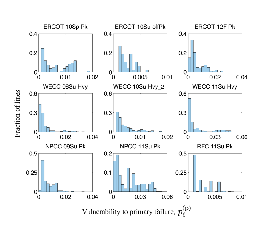
Fig. S7: Vulnerability distribution for individual snapshots. Histograms of the relative frequencies of line vulnerability to primary failure $p_{\ell}^{\text{(p)}}$ within the vulnerable set, for the top three snapshots in each interconnection when ranked by the size $P_{\text{s}}$ of the largest cascade. The abbreviations for the snapshots and the triggering regions are given in Tables S1 and S2, respectively.

To characterize the lines at risk of primary failures, we now shift our attention back to individual transmission lines connecting buses in each snapshot, rather than their collective representation as links. For this purpose, we define a vulnerable transmission line for a given snapshot t o be a line $\ell$ for which $p^{\text{(p)}}_{\ell}>0.0005$ with at least 95% Wilson’s confidence level  (?) (which excludes any line with a single failure in $1{,}000$ simulated events). This approach for vulnerability analysis is in contrast to previous studies on identifying the line failure combinations that initiate large cascading failures (i.e., a single snapshot)  (?, ?). We then define the vulnerable set $\mathcal{V}$ to be the set of all vulnerable lines for the given snapshot. We found that these vulnerable sets not only represented small portions of the grid in each snapshot but also exhibited considerable overlap across different snapshots (although it was rare for the same line to be vulnerable in all snapshots). These findings are presented in Table 1 for each interconnection using, respectively, the weighted average $\langle|{\cal V}|\rangle$ of the number of vulnerable transmission lines over all snapshots and the number $|{\cal V}_{\cap}|$ of lines that were vulnerable in two or more snapshots (relative to the number expected if the vulnerable sets were randomly distributed with no correlation). For example, in the Texas interconnection, $\langle|{\cal V}|\rangle=48$ represents only about $0.6\%$ of all the transmission lines and the relative number of overlapping lines $|{\cal V}_{\cap}|$ is $2.9$. (Details on the distribution of $p^{\text{(p)}}_{\ell}$ for individual snapshots can be found in Fig. S7.)

Having a small portion of the grid vulnerable to cascading failures does not imply that these failures stayed localized even for single snapshots. To quantify the degree to which cascades were localized, we used the concepts of topological distance (the number of links along the shortest paths in the network) and geographical distance (the arc length along the Earth’s surface), both normalized by the size of the triggering region measured by the respective distances and thus are unitless (Materials and Methods, Supplementary Materials). Specifically, the extent of the vulnerable set was measured by $d_{\text{v-v}}$ and $g_{\text{v-v}}$, defined as the normalized topological and geographical distance, respectively, between two transmission lines, averaged over all pairs of lines in the vulnerable set. We further defined $\langle d_{\text{v-v}}\rangle$ and $\langle g_{\text{v-v}}\rangle$ to be the weighted average of $d_{\text{v-v}}$ and $g_{\text{v-v}}$, respectively, over all snapshots. Table 1 shows that, for the Texas and Western networks, both $\langle d_{\text{v-v}}\rangle$ and $\langle g_{\text{v-v}}\rangle$ are comparable with the size of the interconnection, revealing that the spreading of cascades is nonlocal [which is consistent with observations from historical data  (?), from power flow calculations  (?), and from abstract models  (?, ?)]. In all cases $\langle d_{\text{v-v}}\rangle<1$ and $\langle g_{\text{v-v}}\rangle<1$ hold true in the Eastern interconnection, where cascades were actually triggered in a local region and could have, in principle, spread widely to the other regions within the interconnection, leading to $\langle d_{\text{v-v}}\rangle>1$ or $\langle g_{\text{v-v}}\rangle>1$. This suggests that there is also an aspect of the cascading failures that is local: the propagation of failures in general does not extend too far from the region being perturbed.

The analysis of vulnerable sets provide relevant insights not only into the origins of cascading failures, but also into the size of the damage inflicted on the network by individual cascades. In particular, what is the difference between the perturbations that cause large cascades and those that do not? To answer this question quantitatively, we categorized cascades according to their sizes measured by the power shed $P_{\text{s}}$ defined above: small cascades ($0.01\text{MW}\leq P_{\text{s}}<300$MW) and large cascades ($P_{\text{s}}\geq 300$MW). This choice of measure and threshold is based on the NERC requirement that all blackouts causing more than $300$MW of lost power be reported. We characterized perturbations by three different measures based on (normalized) distances: $d_{\text{t-t}}$, defined as the average pairwise distance among the $n_{\text{t}}$ triggering line failures, as well as $d_{\text{t-v}}$ and $g_{\text{t-v}}$, defined as the minimum topological and geographical distances, respectively, from one triggering line failure to the vulnerable set $\mathcal{V}$. Figure 5 shows the average of these distances ($\bar{d}_{\text{t-t}}$, $\bar{d}_{\text{t-v}}$, and $\bar{g}_{\text{t-v}}$) over cascades in each size category for each region. Cascades resulting in power shed $P_{\text{s}}\geq 300\text{MW}$ were associated with a set of triggering line failures that were topologically closer to each other (Fig. 5A), as well as with triggering failures that occurred topologically and geographically closer to a vulnerable line (Fig. 5, B and C).

Conclusions

Our vulnerability analysis of a continent-wide power system distinguishes itself from most previous studies by its scale, but also by accounting for: (i) the physics of cascading failures (DC-approximated power flow redistribution and heating of line conductors); (ii) grid operation practices (generation reserves and power shedding); and (iii) a wide range of conditions across years, seasons, and power demand levels (over which the average cascade size varies by one to two orders of magnitude). A strength of our approach is that it consists of tools—the definition of vulnerable sets, the method for aggregating multiple network conditions, and the analysis of coreness-vulnerability correlations—that are applicable to any cascade-prone network.

Our analysis separates the set of all failures occurring in cascade events into primary failures, which define the vulnerable set and account for only 1/5 of all failures, and secondary failures, which are more uniformly distributed and, albeit more numerous, are a mere consequence of the primary ones. The vulnerable set is not only surprisingly small but also highly skewed—with few lines far more likely to undergo a primary failure than the others—and patchy even when we control for the heterogeneity in the geographic organization of the grid. Although the vulnerable set is widespread through the network, the portion of it recruited in each cascade is not, and is in fact strongly spatially correlated with the location of the triggering line failures; this is counter to the perception that cascades [for being nonlocal with respect to both topological and geographical distances  (?, ?)] can spread essentially without spatial constraints.

Our analysis also shows that larger cascades are associated with co-occurring perturbations that are closer both to each other and to the vulnerable set. This validates the existing hypothesis that localized triggering failures amount to bigger cascades  (?) and reveals a striking relation to the classic threshold model  (?) used to describe behavioral cascades in social systems, where large cascades tend to be triggered by perturbations adjacent to the set of “early adopters.” This set corresponds to the nodes most susceptible to change and thus plays a role similar to the one the vulnerable set plays in our analysis. The network topology emerged as a significant factor in determining the risk of cascading failures in our analysis based on the $k$-core decomposition, which has also been used to characterize nodes that serve as efficient spreaders in contact-based processes  (?).

There are never two identical cascades in a network. It may thus come as a surprise that (primary) failures in large cascades are constrained to only a small subset of the network, which will likely experience new failures in the absence of remediating actions. This offers a scientific foundation for failure-based allocation of resources, which in the case of a power grid would be based on prioritizing upgrades of the system on the basis of previous observed failures  (?)—but only if those are the primary (as opposed to all) failures (although upgrading transmission line capacities in the vulnerable set could create new vulnerable lines outside the set). Future work will be needed to determine the extent to which this applies to other flow networks that are subject to repeated failures, such as supply chains, food webs, and traffic networks.

Methods summary

For each interconnection, the system was modeled as a network of buses connected by transmission lines, given the parameters of individual network components in a given snapshot. The triggering perturbations were chosen uniformly from all lines for the Texas and Western networks, whereas for the Eastern network, they were chosen uniformly within one of the six regions defined by NERC (Fig. 1A and Table S2). The initial state of the network and the redistribution of power flow following a line removal were both calculated by solving an equation that expresses a balance between incoming and outgoing power flows at each bus. Through a temperature evolution equation, the heating of a transmission line was modeled as an exponential convergence to the equilibrium temperature determined by the power flow over that line. Mechanisms responsible for the primary failures occurring in a given simulated cascade were identified using an algorithm we developed to determine the degree to which the change in each generator’s output contribute to changes in individual line power flows.

The density-equalizing transformation used to generate Fig. 3 was determined by estimating the density function for the geographical distribution of nodes and evolving it to a uniform-density equilibrium through a linear diffusion process  (?). The topological and geographical distances between two transmission lines are defined based on the corresponding distances between the buses they connect. Both distances are thus zero between two lines that connect to a common bus. Further details on the formulation of the power flow equation, triggering perturbations, temperature evolution equation, validation of the cascade dynamics model against historical data, calculation of the density-equalizing transformation, algorithm for assigning power flow changes to generators, and the definitions of bus-to-bus distances, are all given in the supplementary materials.

Supplementary materials

Materials and Methods
Figs. S1 to S7
Tables S1 to S3

Table 1. Subdivisions of the U.S.-South Canada power grid and its vulnerable sets. The rows represent the regions defined by NERC (Fig. 1A and Table S2), within which the simulated cascades are triggered. The columns represent the number of buses, number of transmission lines, and four measures of the vulnerable sets: the number of vulnerable lines $|{\cal V}|$, the relative number of lines that are vulnerable in multiple snapshots $|{\cal V}_{\cap}|$, and the mean pairwise normalized topological and geographical distances between vulnerable lines, $d_{\text{v-v}}$ and $g_{\text{v-v}}$, respectively. These quantities are averaged over all snapshots $\bigl{(}$which is indicated by the notation $\langle\,\cdot\,\rangle\bigr{)}$. The normalized distances are defined in Materials and Methods.

Interconnections				Vulnerable sets
	$\langle$Buses$\rangle$	$\langle$Lines$\rangle$		$\langle|{\cal V}|\rangle$	$|{\cal V}_{\cap}|$	$\langle d_{\text{v-v}}\rangle$	$\langle g_{\text{v-v}}\rangle$
Texas	$6{,}161$	$7{,}637$		$48$	$2.9$	$0.82$	$0.70$
Western	$15{,}891$	$20{,}397$		$81$	$5.9$	$0.84$	$0.95$
Eastern	$56{,}740$	$72{,}903$
FRCC				$37$	$1.1$	$0.69$	$0.70$
MRO				$32$	$3.4$	$0.79$	$0.97$
NPCC				$130$	$2.1$	$0.85$	$0.72$
RFC				$76$	$4.5$	$0.94$	$0.91$
SERC				$11$	$11.6$	$0.92$	$0.94$
SPP				$14$	$3.3$	$0.66$	$0.63$

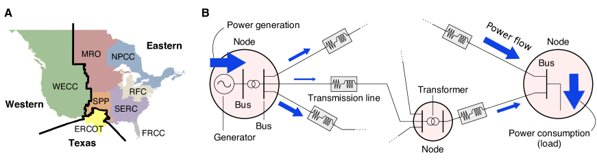
Figure 1: The U.S.-South Canada power transmission network. (A) System map showing the Texas, Western, and Eastern interconnections, as well as the eight NERC regions (Table S2). (B) Schematic diagram of a portion of a transmission network. The vertical lines and pink circles represent buses and nodes, respectively. As indicated by the blue arrows, power injected by the generators flows through this network of transmission lines and is eventually consumed at other points (where the thickness of the arrow represents the amount of power flow).

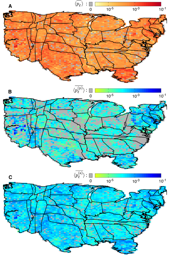
Figure 3: Vulnerability of the power grid on a density-equalizing map. (A) Each pixel is color-coded by the average a-vulnerability $\langle\overline{p^{\phantom{\text{p}}}_{\ell}}\rangle$, including both primary and secondary failures, over all links connected to nodes in the area of the pixel. The cartogram was generated using the diffusion-based method in Ref.  (?) to equalize the density of nodes (Materials and Methods), and is limited to the U.S. portion of the network. Color gray marks the pixels with zero average a-vulnerability. (B and C) Same as in (A) but color-coded separately for the average a-vulnerability to primary failures $\langle\overline{p^{\text{(p)}}_{\ell}}\rangle$ (B) and the average a-vulnerability to secondary failures $\langle\overline{p^{\text{(s)}}_{\ell}}\rangle$ (C).

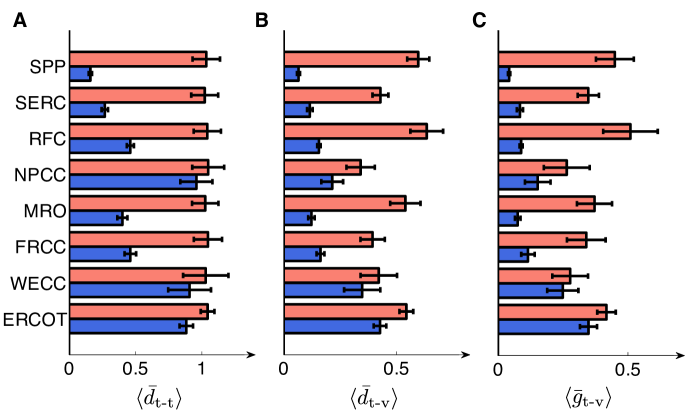
Figure 5: Cascade size and distances involving triggering line failures. (A to C) Three types of (normalized) distances are shown for each NERC region (Fig. 1A and Table S2): the mean pairwise topological distance between the triggering failures (A), the topological distance between the set of triggering failures and the vulnerable set (B), and the geographical distance between the set of triggering failures and the vulnerable set (C). The distances are averaged separately over large cascades (blue, $P_{\text{s}}\geq 300\text{MW}$) and over small cascades (red, $0.01\text{MW}\leq P_{\text{s}}<300\text{MW}$). In each case, the distances are further averaged over all snapshots. Error bars mark the estimated standard deviation.

Supplementary Materials

Materials and Methods

Determining power flow in each interconnection.

Each snapshot of each interconnection is modeled as a network of buses connected by transmission lines, where a bus represents an end point of a transmission line or a coil of a transformer. We extracted the following parameters from the FERC data: the net injected real power at each generator bus, the capacity of each generator, the power demand at each non-generator bus, as well as the parameters of each transmission line and transformer (including their impedance and long-term capacity rating). A transformer is modeled as a transmission line $\ell$ connecting two buses ($i$ and $j$), where the voltage ratio between these points determines the tap ratio $\tau_{\ell}$ of this line, and the phase shift of the transformer determines the antisymmetric phase shift matrix $\Delta=(\Delta_{ij})$; transformers can thus fail in a cascade due to overheating. The state of the network can be represented by the complex voltage $V_{i}=|V_{i}|e^{j\Theta_{i}}$ at each bus $i$, which in a steady state is determined by the power flow equation $V_{i}\cdot I^{*}_{i}=S_{i}^{\text{(g)}}-S_{i}^{\text{(d)}}$, where $I^{*}_{i}$ is the conjugate of the injected complex current, $S_{i}^{\text{(g)}}=P_{i}^{\text{(g)}}+jQ_{i}^{\text{(g)}}$ is the complex power produced (by the connected generators), $S_{i}^{\text{(d)}}=P_{i}^{\text{(d)}}+jQ_{i}^{\text{(d)}}$ is the power consumed (as determined by load demand), and $j:=\sqrt{-1}$ is the imaginary unit. The vector of current injections $I=(I_{i})$ is determined by the admittance matrix $Y$ of the network through $I=Y\cdot V$, where $Y$ is a Laplacian matrix whose off-diagonal element $Y_{ij}$ is the negative of the admittance of the lines connecting $i$ and $j$. In a steady state, the total power generated in the network is equal to the total power consumed. Invoking the DC approximation (42), which assumes that the line resistance is negligible and the voltage magnitudes can be approximated as $|V_{i}|\approx 1$ (per unit), we linearize the power flow equation to obtain $P^{\text{(g)}}-P^{\text{(d)}}=B\cdot\Theta-P^{\text{shift}}$ for the real power. Here $\Theta=(\Theta_{i})$ is the vector of phase angles, $P^{\text{shift}}=(P^{\text{shift}}_{i})$ is vector of the phase shifts, $B$ is a Laplacian matrix with off-diagonal elements $B_{ij}=-1/(\tau_{\ell}x_{\ell})$, parameter $x_{\ell}$ is the line or transformer reactance, and the tap ratio $\tau_{\ell}=1$ for non-transformer lines. The component $P^{\text{shift}}_{i}$ represents the phase shift at bus $i$ and is determined by the phase shifts (if any) over all the transmission lines connecting to it: $P^{\text{shift}}_{i}=\sum_{j\in\mathscr{B}(i)}\Delta_{ij}$, where $\mathscr{B}(i)$ is the set of first neighbors of $i$. Then, with $\Theta$ determined by the linearized power flow equation, we can approximate the real power flowing on the line $\ell$ from bus $i$ to $j$ by $\dfrac{1}{\tau_{\ell}x_{\ell}}(\Theta_{i}-\Theta_{j}-\Delta_{ij})$.

Triggering perturbation.

For a given snapshot of a given interconnection, we model the initial perturbation that triggers a cascade event as the removal of a fixed number $n_{\text{t}}$ of randomly chosen transmission lines. For the Texas and Western interconnections, we choose these lines uniformly from all lines present in the snapshot. For the Eastern interconnection (the largest of the three), we constrain the line selection to one of the six regions defined by NERC (Fig. 1A and Table S2), but with the event then evolved through the entire interconnection. This choice accounts for the intuition that failures in geographical proximity are more likely to trigger large cascades, which we quantitatively verified (Fig. 5) and is consistent with the empirical observation that blackout-causing perturbations tend to be localized (3).

Modeling cascade dynamics.

Each iteration of our simulation begins with the removal of a line that models an overload failure (or of the $n_{\text{t}}$ lines chosen as the initial perturbation for the first iteration). If the network remains connected after the removal, the redistribution of power flow is calculated by solving the DC power flow equation, as described in a section above. The DC approximation offers the computational efficiency that allows for the simulation of cascading failures in large-scale networks and is commonly used in the engineering community (13, 14, 24, 25). If the grid separates into isolated sub-grids after the line removal, the following procedure is taken to rebalance supply and demand, which allows for the calculation of the redistributed power flow. For each sub-grid with unbalanced total power generation and consumption, we first select a generator with the largest capacity as a “slack bus” (a generator whose output can be adjusted between zero and its maximum generation output on short time scales) and adjust its output as much as possible within the range allowed; the slack bus models the role of generation reserves typically designed into real power grids. If this does not result in balanced supply and demand in a sub-grid, we uniformly scale down the output of all generators or the consumption (load) at all buses in the sub-grid to achieve a balance, depending on whether the supply is larger or smaller than the demand. The latter case, in which the total consumption is reduced, models power shedding procedures used by grid operators. Applying this procedure to all isolated sub-grids, we obtain the redistributed power flow over the network.

Given the redistributed power flow, the next line outage (if any) is identified by modeling the heating of line conductors using a temperature-evolution model (12). Specifically, the temperature of line $\ell$ at time $t$ (measured from the time of flow redistribution within this iteration) is determined by its power flow $P_{\ell}$ through

$$T_{\ell}(t)=e^{-\mu t}\big{(}T_{\ell}(0)-T_{\text{e}}(P_{\ell})\big{)}+T_{\text{e}}(P_{\ell}),$$ (S1)

where $T_{\text{e}}(P_{\ell}):=\frac{\alpha}{\mu}P_{\ell}^{2}+T_{\text{a}}$ is the equilibrium temperature [to which $T_{\ell}(t)$ approaches as $t\to\infty$ according to Eq. (S1)], the constants $\mu$ and $\alpha$ are determined by the properties of the line (assumed to be the same for all $\ell$ for simplicity), and $T_{\text{a}}$ is the ambient temperature. This is a simplified version of the temperature-evolution model used in Ref. (12). Similar temperature models have also been used for IEEE test systems in recent studies focusing on mitigating cascades (43) and evaluating cascade risk (44). The capacity of the line $P^{\max}_{\ell}$ (extracted from the dataset) is associated with the critical temperature $T^{\star}_{\ell}:=T_{\text{e}}(P^{\max}_{\ell})$ above which the line would become overheated. According to Eq. (S1), sustained power flow $P_{\ell}>P^{\max}_{\ell}$ would bring the line temperature to the critical temperature $T^{\star}_{\ell}$ at $t=t^{\star}_{\ell}:=-\frac{1}{\mu}\ln\frac{T^{\star}_{\ell}-T_{\text{e}}(P_{\ell})}{T_{\ell}(0)-T_{\text{e}}(P_{\ell})}$. When this occurs, we remove line $\ell$ from the network (primary line failure) to model the action of a protective relay that automatically shuts down the line to prevent permanent damage. Note that the critical temperature $T^{\star}_{\ell}$ serves as a proxy for other failure criteria, such as those based on various stability considerations. The next iteration then begins with the removal of the line with the smallest $t^{\star}_{\ell}$, followed by the update of the temperature of all the other lines to the value given by Eq. (S1) for $t=\min_{\ell}t^{\star}_{\ell}$ and the recalculation of the power flow.

We repeat this process of line removal and power flow redistribution until no line is overheated (i.e., $T_{\text{e}}(P_{\ell})\leq T^{\star}_{\ell}$ or, equivalently, $P_{\ell}\leq P^{\max}_{\ell}$, for all $\ell$), which generates a (finite) sequence of line failures with time stamps, along with the total power shed. At the beginning of the cascade event, the temperature of all lines are assumed to be equal to the ambient temperature, $T_{\ell}(0)=T_{\text{a}}$ for all $\ell$, which ensures that the failure sequence and power shed do not depend on $T_{\text{a}}$, $\alpha$, or $\mu$.

Model validation.

We validated the cascade model against available historical data on cascades in the Western interconnection. We compared the size of cascades from simulations and from the observed real events in terms of two different measures: the number of primary line failures $N_{\text{f}}$ and the power shed $P_{\text{s}}$. Considering the scarcity of public data on line outages (primary failures), we used the portion of the Western interconnection represented in the BPA data as a proxy for the entire network. Following the criteria in Ref. (45), we identified the individual cascades by grouping the outages based on their temporal proximity, which resulted in $5{,}227$ cascade events from the recorded $8{,}864$ transmission line outages, each triggered by a set of varying number of line failures that was also identified from the data. To compare with this historical data, we simulated cascades using all available snapshots of the Western interconnection. For this purpose the number of triggers $n_{\text{t}}$ is chosen randomly following the probability distribution $P(n_{\text{t}})$ estimated from the data. We generated a total of $10^{6}$ simulated events, with the numbers for individual snapshots chosen to be proportional to the weights in Table S1. Figure S1A shows that the sample distribution of cascade sizes generated from these simulations is in good agreement with the distribution from real events when measured in terms of $N_{\text{f}}$.

The NERC data includes $190$ power outages reported between years 1984 and 2006, among which $93$ cascade events have power shed larger than $300$MW. The dataset formed by these $93$ large cascades is believed to be complete and reliable given the NERC requirement on the reporting of cascades resulting in $\geq\!300$MW uncontrolled load. Using both the BPA and NERC data, we also validated the extremal cascade size (in terms of $N_{\text{f}}$ and $P_{\text{s}}$, respectively) in our simulations against the historical data (Fig. S1, B and C).

Density-equalizing maps.

In the diffusion-based algorithm of Ref. (41), the distribution of nodes is represented by a density function $\rho(\vec{r})$ and is then evolved to a uniform-density equilibrium through a linear diffusion process. The displacements of nodes by this diffusion process determine the transformation of the original map into a properly scaled density-equalizing cartogram. In our implementation used in Fig. 3, the density of nodes was calculated with respect to a fine-grained $200\times 200$ grid of a box including the entire U.S.-South Canada power grid ($24.56^{\circ}$N–$59.15^{\circ}$N, $130.35^{\circ}$W–$59.87^{\circ}$W) in the rectangular map projection. To control the distortion and facilitate interpretation of the result, we focused on the U.S. portion of the grid and assigned a constant nonzero density everywhere outside the U.S. border.

Identifying mechanisms responsible for primary failures.

In our cascade model, a given primary failure is caused either by the rerouting of power flow that occurs following the previous primary failure or by the adjustment of generator outputs that may occur when a part of the grid becomes disconnected from the rest (noting that consumption is only adjusted downwards and thus cannot by itself cause overloading). If the grid does not become disconnected, then flow rerouting must be responsible for the failure. If the grid becomes disconnected, the mechanism can be either flow rerouting, generator output adjustment, or both. In that case, we quantify the extent to which flow rerouting has caused the failure using the following algorithm. Let $P_{\ell}(k)$ denote the power flow carried by line $\ell$ at the end of the $k$th iteration (just before the next line removal) and let $\Delta_{\ell}(k):=P_{\ell}(k+1)-P_{\ell}(k)$ be the total flow change on line $\ell$ from the $k$th to the $(k+1)$th iteration. Then, the fraction $f_{\ell i}$ of the flow $P_{\ell}(k)$ that is supplied by generator $i$ can be defined and computed using a flow tracing algorithm based on a proportional sharing principle (46). This fraction can be used to determine the amount of flow change $\Delta^{(\text{g})}_{\ell i}(k)$ that can be attributed to the adjustment of generator $i$ as $\Delta^{(\text{g})}_{\ell i}(k):=f_{\ell i}\Delta P^{(\text{g})}_{i}(k)$, where $\Delta P^{(\text{g})}_{i}(k)$ denotes the change in the output of generator $i$ in this iteration. The total amount of flow change caused by the generation adjustments is then $\Delta^{(\text{g})}_{\ell}(k):=\sum_{i}\Delta^{(\text{g})}_{\ell i}(k)$. Thus, $\Delta^{(\text{g})}_{\ell}(k)$ quantifies the degree to which generation changes have contributed to the failure, if line $\ell$ fails at the beginning of the $(k+1)$th iteration. The contribution of flow rerouting to the failure is then measured by $\Delta^{(\text{r})}_{\ell}(k):=\Delta_{\ell}(k)-\Delta^{(\text{g})}_{\ell}(k)$. If the grid were not disconnected in that iteration, we would have $\Delta^{(\text{g})}_{\ell}(k)=0$ and $\Delta^{(\text{r})}_{\ell}(k)=\Delta_{\ell}(k)$, since the whole change would have been due to rerouting. To account for cases in which a line continues to be overloaded for multiple iterations before experiencing a primary failure, we keep track of running totals $\widetilde{\Delta}^{(\text{r})}_{\ell}:=\sum_{k}\Delta^{(\text{r})}_{\ell}(k)$, $\widetilde{\Delta}^{(\text{g})}_{\ell}:=\sum_{k}\Delta^{(\text{g})}_{\ell}(k)$, and $\widetilde{\Delta}_{\ell}:=\sum_{k}\Delta_{\ell}(k)$ for each $\ell$, where the sums are taken over the most recent set of consecutive iterations in which the line has been overloaded. If, at the time of a primary failure, $\widetilde{\Delta}^{(\text{r})}_{\ell}$ and $\widetilde{\Delta}_{\ell}$ have the same sign but $\widetilde{\Delta}^{(\text{g})}_{\ell}$ has the opposite sign (or $\widetilde{\Delta}^{(\text{g})}_{\ell}=0$), then flow rerouting must be solely responsible for the failure (as $\widetilde{\Delta}^{(\text{g})}_{\ell}$ can only help prevent overloading in that case). Using the 2010 spring peak snapshot of the Texas grid as a representative example, we counted the number of primary failures for which this was the case among all primary failures observed in $5{,}000$ simulated cascade events. We found this number to be $2{,}222$ out of $2{,}257$ observed primary failures, indicating that rerouting of power flow was solely responsible for over $98$% of these primary failures.

Distances between transmission lines.

To define the topological and geographical distances between two lines, we start from the corresponding notions of distance between two buses. The topological distance $d_{ij}$ is defined as the number of lines along the shortest path between buses $i$ and $j$ in the network. The geographical distance $g_{ij}$ is defined as the arc length between buses $i$ and $j$ along the Earth’s great circle. The topological distance $d_{\ell\ell^{\prime}}$ between line $\ell$ (connecting bus $i$ to $j$) and line $\ell^{\prime}$ (connecting bus $i^{\prime}$ to $j^{\prime}$) is defined as the minimum of the set $\{d_{ii^{\prime}},d_{ij^{\prime}},d_{ji^{\prime}},d_{jj^{\prime}}\}$. The distance between line $\ell$ and a set of lines $S$ is defined as $\min_{\ell^{\prime}\in S}\{d_{\ell\ell^{\prime}}\}$ and the distance between two sets, $S$ and $S^{\prime}$, is defined as $\min_{\ell\in S,\ell^{\prime}\in S^{\prime}}\{d_{\ell\ell^{\prime}}\}$. The geographical distances are defined similarly, with each $d$ replaced by $g$ in the notations. When calculating these distances in our characterization of cascading failures, we normalize them by the average pairwise distance between any two lines in the corresponding NERC region where the cascade events are triggered.

Supplementary Figures

 

Supplementary Tables

Table S1: Case description of the available snapshots of the U.S.-South Canada power grid and simulation details.

Interconnection	Snapshot	Acronym	Buses	Generators	Lines	Load (MW)	$K$	$w_{c}$
Texas	2010 spring peak	10Sp Pk	$5{,}960$	$651$	$7{,}334$	$61{,}397$	$5{,}000$	$1/24$
	2010 spring off-peak	10Sp offPk	$5{,}959$	$651$	$7{,}331$	$37{,}737$	$5{,}000$	$1/24$
	2010 summer peak	10Su Pk	$6{,}005$	$658$	$7{,}395$	$72{,}095$	$5{,}000$	$1/24$
	2010 summer off-peak	10Su offPk	$6{,}005$	$660$	$7{,}395$	$42{,}239$	$5{,}000$	$1/24$
	2010 fall peak	10F Pk	$6{,}010$	$668$	$7{,}401$	$57{,}663$	$5{,}000$	$1/24$
	2010 fall off-peak	10F offPk	$6{,}010$	$663$	$7{,}401$	$35{,}342$	$5{,}000$	$1/24$
	2011 winter peak	11W Pk	$6{,}012$	$665$	$7{,}407$	$57{,}252$	$5{,}000$	$1/24$
	2011 winter off-peak	11W offPk	$6{,}012$	$665$	$7{,}407$	$38{,}045$	$5{,}000$	$1/24$
	2011 spring peak	11Sp Pk	$6{,}034$	$677$	$7{,}451$	$56{,}597$	$5{,}000$	$1/24$
	2011 spring off-peak	11Sp offPk	$6{,}034$	$679$	$7{,}451$	$34{,}698$	$5{,}000$	$1/24$
	2011 summer peak	11Su Pk	$6{,}057$	$682$	$7{,}493$	$70{,}313$	$5{,}000$	$1/24$
	2011 summer off-peak	11Su offPk	$6{,}057$	$684$	$7{,}493$	$40{,}028$	$5{,}000$	$1/24$
	2011 fall peak	11F Pk	$6{,}062$	$690$	$7{,}489$	$55{,}625$	$5{,}000$	$1/24$
	2011 fall off-peak	11F offPk	$6{,}063$	$691$	$7{,}491$	$34{,}148$	$5{,}000$	$1/24$
	2012 winter peak	12W Pk	$6{,}066$	$691$	$7{,}506$	$55{,}951$	$5{,}000$	$1/24$
	2012 winter off-peak	12W offPk	$6{,}066$	$691$	$7{,}506$	$37{,}305$	$5{,}000$	$1/24$
	2012 spring peak	12Sp Pk	$6{,}405$	$646$	$8{,}006$	$56{,}926$	$5{,}000$	$1/24$
	2012 spring off-peak	12Sp offPk	$6{,}405$	$646$	$8{,}006$	$34{,}778$	$5{,}000$	$1/24$
	2012 summer peak	12Su Pk	$6{,}428$	$648$	$8{,}039$	$72{,}442$	$5{,}000$	$1/24$
	2012 summer off-peak	12Su offPk	$6{,}428$	$648$	$8{,}039$	$40{,}934$	$5{,}000$	$1/24$
	2012 fall peak	12F Pk	$6{,}432$	$649$	$8{,}043$	$57{,}441$	$5{,}000$	$1/24$
	2012 fall off-peak	12F offPk	$6{,}432$	$649$	$8{,}043$	$34{,}810$	$5{,}000$	$1/24$
	2013 winter peak	13W Pk	$6{,}459$	$667$	$8{,}075$	$60{,}209$	$5{,}000$	$1/24$
	2013 winter off-peak	13W offPk	$6{,}459$	$667$	$8{,}075$	$39{,}345$	$5{,}000$	$1/24$
Western	2008 heavy winter	08W Hvy	$15{,}387$	$2{,}997$	$19{,}687$	$128{,}331$	$6{,}000$	$3/24$
	2008 heavy spring	08Sp Hvy	$15{,}439$	$3{,}017$	$19{,}752$	$113{,}824$	$6{,}000$	$6/24$
	2008 heavy summer	08Su Hvy	$15{,}722$	$3{,}065$	$20{,}037$	$159{,}890$	$6{,}000$	$1/24$
	2010 heavy summer	10Su Hvy	$16{,}932$	$3{,}189$	$20{,}476$	$163{,}174$	$6{,}000$	$(1/2){\cdot}1/24$
	2010 heavy summer_ 2	10Su Hvy_ 2	$16{,}796$	$3{,}292$	$21{,}269$	$168{,}091$	$6{,}000$	$(1/2){\cdot}1/24$
	2011 light spring	11Sp Lgt	$16{,}082$	$3{,}181$	$20{,}711$	$98{,}415$	$6{,}000$	$12/24$
	2011 heavy summer	11Su Hvy	$17{,}524$	$3{,}467$	$22{,}510$	$194{,}983$	$6{,}000$	$1/24$
Eastern	2009 winter peak	09W Pk	$53{,}887$	$7{,}683$	$69{,}431$	$548{,}727$	$23{,}000$	$1/24$
	2009 spring peak	09Sp Pk	$53{,}649$	$7{,}645$	$69{,}179$	$460{,}594$	$23{,}000$	$1/24$
	2009 summer peak	09Su Pk	$54{,}025$	$7{,}614$	$69{,}697$	$641{,}388$	$23{,}000$	$1/24$
	2009 fall peak	09F Pk	$53{,}866$	$7{,}676$	$69{,}495$	$474{,}961$	$23{,}000$	$(3/2){\cdot}1/24$
	2009 light load	09 Lgt	$53{,}651$	$7{,}584$	$69{,}182$	$286{,}672$	$23{,}000$	$6/24$
	2010 winter peak	10W Pk	$56{,}714$	$7{,}932$	$72{,}935$	$538{,}747$	$23{,}000$	$1/24$
	2010 spring peak	10Sp Pk	$56{,}422$	$7{,}847$	$72{,}519$	$452{,}769$	$23{,}000$	$1/24$
	2010 summer shoulder	10Su Shl	$56{,}616$	$7{,}804$	$72{,}780$	$492{,}851$	$23{,}000$	$(1/2){\cdot}1/24$
	2010 summer peak	10S Pk	$56{,}642$	$7{,}805$	$72{,}811$	$622{,}180$	$23{,}000$	$(1/2){\cdot}1/24$
	2011 winter peak	11W Pk	$60{,}073$	$8{,}137$	$76{,}942$	$537{,}272$	$23{,}000$	$1/24$
	2011 spring peak	11Sp Pk	$59{,}741$	$8{,}044$	$76{,}487$	$456{,}678$	$23{,}000$	$1/24$
	2011 summer shoulder	11Su Shl	$59{,}943$	$8{,}027$	$76{,}791$	$490{,}586$	$23{,}000$	$(1/2){\cdot}1/24$
	2011 summer peak	11Su Pk	$59{,}948$	$8{,}043$	$76{,}798$	$616{,}200$	$23{,}000$	$(1/2){\cdot}1/24$
	2011 fall peak	11F Pk	$59{,}966$	$8{,}089$	$76{,}798$	$467{,}659$	$23{,}000$	$(3/2){\cdot}1/24$
	2011 light load	11 Lgt	$59{,}669$	$7{,}993$	$76{,}395$	$269{,}961$	$23{,}000$	$6/24$

The description of each snapshot follows the terminology in the FERC Form 715 and is abbreviated to facilitate referencing in this article. The number of buses, number of generators, number of transmission lines, and the amount of load vary across different snapshots. Unless noted otherwise, our simulation results are based on $K$ simulated events in which the network is perturbed by the removal of $n_{\text{t}}=3$ randomly selected transmission lines within the same region. For the Eastern interconnection, which consists of six regions (Fig. 1A and Table S2) the $23{,}000$ simulations are distributed approximately proportionally to the number of transmission lines in each region: FRCC ($1{,}200$), MRO ($3{,}400$), NPCC ($4{,}000$), RFC ($6{,}400$), SERC ($6{,}000$), and SPP ($2{,}000$). The last column lists the relative weights assigned to each snapshot in our calculations of averages, chosen to give comparable weights across the different seasons as well as to high and low power demand conditions.

Table S2: Names, abbreviations, and basic properties of the NERC reliability regions.

Interconnection	Region	Buses	Lines	Load (MW)
Texas	Electric Reliability Council of Texas (ERCOT)	$\enskip 5{,}959$ – $\enskip 6{,}459$	$\enskip 7{,}331$ – $\enskip 8{,}075$	$34{,}148$ – $\enskip 72{,}442$
Western	Western Electricity Coordinating Council (WECC)	$15{,}387$ – $17{,}524$	$19{,}687$ – $22{,}510$	$98{,}415$ – $194{,}983$
Eastern	Florida Reliability Coordinating Council (FRCC)	$\enskip 2{,}945$ – $\enskip 3{,}022$	$\enskip 3{,}795$ – $\enskip 3{,}914$	$17{,}845$ – $\enskip 49{,}608$
	Midwest Reliability Organization (MRO)	$\enskip 7{,}605$ – $\enskip 8{,}340$	$\enskip 9{,}370$ – $10{,}297$	$24{,}601$ – $\enskip 49{,}275$
	Northeast Power Coordinating Council (NPCC)	$\enskip 9{,}381$ – $10{,}784$	$12{,}609$ – $14{,}054$	$42{,}398$ – $\enskip 92{,}524$
	ReliabilityFirst Corporation (RFC)	$14{,}896$ – $17{,}497$	$19{,}753$ – $23{,}152$	$81{,}970$ – $201{,}736$
	SERC Reliability Corporation (SERC)	$13{,}751$ – $15{,}320$	$17{,}637$ – $19{,}444$	$84{,}676$ – $211{,}561$
	Southwest Power Pool Regional Entity (SPP)	$\enskip 4{,}969$ – $\enskip 5{,}161$	$\enskip 5{,}908$ – $\enskip 6{,}126$	$14{,}203$ – $\enskip 38{,}894$
For each property, we show the minimum and the maximum over all snapshots in our dataset (listed in Table S1).

Table S3: Number of links experiencing primary and secondary failures.

Interconnection	Nodes	Links	$N^{\text{(p)}}$	$N^{\text{(s)}}$	$\frac{N^{\text{(s)}}}{N^{\text{(p)}}}$
Texas	$3{,}275$	$6{,}664$	$811$	$3{,}274$	$4.04$
Western	$9{,}658$	$21{,}589$	$2{,}443$	$9{,}773$	$4.00$
Eastern	$27{,}822$	$54{,}846$	$5{,}726$	$20{,}798$	$3.63$
FRCC	$1{,}598$	$3{,}188$	$988$	$2{,}306$	$2.33$
MRO	$3{,}972$	$6{,}952$	$668$	$3{,}150$	$4.72$
NPCC	$3{,}253$	$7{,}758$	$1{,}725$	$5{,}120$	$2.97$
RFC	$8{,}247$	$17{,}674$	$2{,}234$	$7{,}328$	$3.28$
SERC	$8{,}619$	$17{,}969$	$653$	$4{,}335$	$6.64$
SPP	$2{,}501$	$5{,}312$	$440$	$2{,}136$	$4.85$
Total	$40{,}755$	$83{,}099$	$8{,}980$	$33{,}845$	$3.77$

We show the number of links $N^{\text{(p)}}$ $\bigl{(}N^{\text{(s)}}\bigr{)}$ whose a-vulnerability to primary (secondary) failures was nonzero in our simulations for each NERC region in which cascade events were triggered, along with the total for the entire network. Among the $83{,}099$ links in the network, the number of links that experienced primary failures was $8{,}980$ ($10.8\%$). For the Eastern interconnection, there are overlaps between the failed links in cascades triggered from different regions, which is the reason why the number of links that fail in the entire interconnection is smaller than the corresponding number summed over the six regions. For comparison, the second and third columns list the total number of nodes and links, respectively. For the Eastern interconnection, these totals are also smaller than the corresponding sums over the individual regions, in this case because some small portions of the grid belong to different NERC regions at different times.

References and Notes

- 1. The U.S. Department of Energy, http://www.energy.gov.
- 2. K. H. LaCommare, J. H. Eto, Cost of power interruptions to electricity consumers in the United States (US). Energy 31, 1845–1855 (2006).
- 3. P. Hines, J. Apt, S. Talukdar, Large blackouts in North America: Historical trends and policy implications. Energ. Policy 37, 5249–5259 (2009).
- 4. D. J. Watts, A simple model of global cascades on random networks. Proc. Natl. Acad. Sci. USA 99, 5766–5771 (2002).
- 5. K. I. Goh, D.-S. Lee, B. Kahng, D. Kim, Sandpile on scale-free networks. Phys. Rev. Lett. 91, 148701 (2003).
- 6. P. Crucitti, V. Latora, M. Marchiori, Model for cascading failures in complex networks. Phys. Rev. E 69, 045104 (2004).
- 7. A. E. Motter, Cascade control and defense in complex networks. Phys. Rev. Lett. 93, 098701 (2004).
- 8. R. Kinney, P. Crucitti, R. Albert, V. Latora, Modeling cascading failures in the North American power grid. Euro. Phys. J. B 46, 101–107 (2005).
- 9. S. V. Buldyrev, R. Parshani, G. Paul, H. E. Stanley, S. Havlin, Catastrophic cascade of failures in interdependent networks. Nature 464, 1025–1028 (2010).
- 10. C. D. Brummitt, R. M. D’Souza, E. A. Leicht, Suppressing cascades of load in interdependent networks. Proc. Natl. Acad. Sci. USA 109, E680–E689 (2012).
- 11. D. P. Nedic, I. Dobson, D. S. Kirschen, B. A. Carreras, V. E. Lynch, Criticality in a cascading failure blackout model. Int. J. Elec. Power 28 627–633 (2006).
- 12. M. Anghel, K. A. Werley, A. E. Motter, Stochastic model for power grid dynamics. Proceedings of the 40th Annual Hawaii International Conference on System Sciences HICSS’07, Waikoloa, Big Island, HI, USA, Vol. 1, 113 (2007).
- 13. I. Dobson, B. A. Carreras, V. E. Lynch, D. E. Newman, Complex systems analysis of series of blackouts: Cascading failure, critical points, and self-organization. Chaos 17, 026103 (2007).
- 14. A. Bernstein, D. Bienstock, D. Hay, M. Uzunoglu, G. Zussman, Sensitivity analysis of the power grid vulnerability to large-scale cascading failures. Perf. E. R. Si. 40, 33–37 (2012).
- 15. C. Moore, S. Mertens, The Nature of Computation (Oxford University Press, 2011).
- 16. S. H. Strogatz, Exploring complex networks. Nature 410, 268–276 (2001).
- 17. A. Vespignani, Predicting the behavior of techno-social systems. Science 325, 425–428 (2009).
- 18. D. Helbing, Globally networked risks and how to respond. Nature 497, 51–59 (2013).
- 19. S. Sahasrabudhe, A. E. Motter, Rescuing ecosystems from extinction cascades through compensatory perturbations. Nature Commun. 2, 170 (2011).
- 20. J. A. Estes, J. Terborgh, J. S. Brashares, M. E. Power, J. Berger, W. J. Bond, D. A. Wardle, Trophic downgrading of planet Earth. Science 333, 301–306 (2011).
- 21. A. D. Barnosky, E. A. Hadly, J. Bascompte, E. L. Berlow, J. H. Brown, M. Fortelius, A. B. Smith, Approaching a state shift in Earth’s biosphere. Nature 486, 52–58 (2012).
- 22. P. Gai, S. Kapadia, Contagion in financial networks. Proc. R. Soc. A 466, 2401–2423 (2010).
- 23. A. G. Haldane, R. M. May, Systemic risk in banking ecosystems. Nature 469, 351–355 (2011).
- 24. I. Dobson, B. A. Carreras, V. E. Lynch, D. E. Newman, An initial model for complex dynamics in electric power system blackouts. Proceedings of the 34th Annual Hawaii International Conference on System Sciences HICSS’01, Maui, HI, USA, Vol. 2, 2017 (2001).
- 25. M. J. Eppstein, P. Hines, A “random chemistry” algorithm for identifying collections of multiple contingencies that initiate cascading failure. IEEE T. Power Syst. 27, 1698–1705 (2012).
- 26. S. B. Seidman, Network structure and minimum degree. Soc. Networks 5, 269–287 (1983).
- 27. B. Bollobás, The evolution of sparse graphs. Graph Theory and Combinatorics, Proc. Cambridge Combinatorial Conf. in honor of Paul Erdős, 35–57 (Academic Press, 1984).
- 28. S. N. Dorogovtsev, A. V. Goltsev, J. F. F. Mendes, -core organization of complex networks. Phys. Rev. Lett 96, 040601 (2006).
- 29. J. I. Alvarez-Hamelin, L. Dall’Asta, A. Barrat, A. Vespignani, Large scale networks fingerprinting and visualization using the -core decomposition. Adv. Neur. In. 18, 41–50 (2006).
- 30. J. A. Bondy, U. S. R. Murty, Graph Theory with Applications (Macmillan, 1976).
- 31. Y. Yang, T. Nishikawa, A. E. Motter, Vulnerability and cosusceptibility determine the size of network cascades. Phys. Rev. Lett. 118, 048301 (2017).
- 32. L. D. Brown, T. T. Cai, A. DasGupta, Interval estimation for a binomial proportion. Stat. Sci. 16, 101–117 (2001).
- 33. C. Long, D. You, J. Hu, G. Wang, M. Dong, Quick and effective multiple contingency screening algorithm based on long-tailed distribution. IET Gener. Transm. Dis. 10, 257–262 (2016).
- 34. I. Dobson, B. A. Carreras, D. E. Newman, J. M. Reynolds-Barredo, Obtaining statistics of cascading line outages spreading in an electric transmission network from standard utility data. IEEE T. Power Syst. 31, 4831–4841 (2016).
- 35. D. Jung, S. Kettemann, Long-range response in ac electricity grids. Phys. Rev. E 94, 012307 (2016).
- 36. L. Daqing, J. Yinan, K. Rui, S. Havlin, Spatial correlation analysis of cascading failures: Congestions and blackouts. Sci. Rep. 4, 5384 (2014).
- 37. D. Witthaut, M. Timme, Nonlocal effects and countermeasures in cascading failures. Phys. Rev. E 92, 032809 (2015).
- 38. P. D. Hines, I. Dobson, P. Rezaei, Cascading power outages propagate locally in an influence graph that is not the actual grid topology. IEEE T. Power Syst. 32, 958–967 (2017).
- 39. Y. Berezin, A. Bashan, M. M. Danziger, D. Li, S. Havlin, Localized attacks on spatially embedded networks with dependencies. Sci. Rep. 5, 8934 (2015).
- 40. M. Kitsak, L. K. Gallos, S. Havlin, F. Liljeros, L. Muchnik, H. E. Stanley, H. A. Makse, Identification of influential spreaders in complex networks. Nat. Phys. 6, 888–893 (2010).
- 41. M. T. Gastner, M. E. J. Newman, Diffusion-based method for producing density-equalizing maps. Proc. Natl. Acad. Sci. USA 101, 7499–7504 (2004).
- 42. A. J. Wood, B. F. Wollenberg, Power Generation, Operation, and Control (John Wiley & Sons, 2nd ed., 2012).
- 43. M. Almassalkhi, I. Hiskens, Model-predictive cascade mitigation in electric power systems with storage and renewables—Part I: Theory and implementation. IEEE T. Power Syst. 30, 67–77 (2015).
- 44. Q. Chen, L. Mili, Composite power system vulnerability evaluation to cascading failures using importance sampling and antithetic variates. IEEE T. Power Syst. 28, 2321–2330 (2013).
- 45. B. A. Carreras, D. E. Newman, I. Dobson, N. S. Degala, Validating OPA with WECC data. Proc. 46th Annual Hawaii Int. Conf. Syst. Sci., 2197–2204 (IEEE, 2013).
- 46. J. Bialek, Identification of source-sink connections in transmission networks. Fourth International Conference on Power System Control and Management, 200–204 (IET, 1996).
- 47. F. J. Massey, Jr., The Kolmogorov-Smirnov test for goodness of fit. J. Amer. Statist. Assoc. 46, 68–78 (1951).
- 48. B. W. Silverman, Density Estimation for Statistics and Data Analysis (Chapman and Hall, 1986).
- 49. E. J. Gumbel, Statistics of Extremes (Columbia University Press, 1958).
Acknowledgments
The authors thank Hamed Valizadehhaghi for insightful discussions. This work was supported by the Institute for Sustainability and Energy at Northwestern (ISEN) under a Booster Award, the U.S. National Science Foundation under Grant DMS-1057128, and the Advanced Research Projects Agency–Energy (U.S. Department of Energy) under Award Number DE-AR0000702. The views and opinions of authors expressed herein do not necessarily state or reflect those of the United States Government or any agency thereof. The power-grid data were obtained from FERC under a non-disclosure agreement by following the procedure described at https://www.ferc.gov/legal/ceii-foia/ceii.asp. The BPA line outage data and the NERC grid disturbance data are both publicly available at https://transmission.bpa.gov/Business/Operations/Outages/ (Miscellaneous Outage Data and Analysis) and https://www.oe.netl.doe.gov/OE417_annual_summary.aspx (Electric Disturbance Events, OE-417), respectively. The 2010 U.S. census data and the boundary data for the U.S. counties can be downloaded from https://factfinder.census.gov/ and https://www.census.gov/geo/maps-data/data/cbf/cbf_counties.html, respectively.