Deep Object Co-Segmentation

Abstract

This work presents a deep object co-segmentation (DOCS) approach for segmenting common objects of the same class within a pair of images. This means that the method learns to ignore common, or uncommon, background stuff and focuses on common objects. If multiple object classes are presented in the image pair, they are jointly extracted as foreground. To address this task, we propose a CNN-based Siamese encoder-decoder architecture. The encoder extracts high-level semantic features of the foreground objects, a mutual correlation layer detects the common objects, and finally, the decoder generates the output foreground masks for each image. To train our model, we compile a large object co-segmentation dataset consisting of image pairs from the PASCAL dataset with common objects masks. We evaluate our approach on commonly used datasets for co-segmentation tasks and observe that our approach consistently outperforms competing methods, for both seen and unseen object classes.

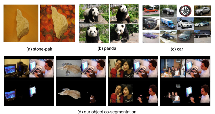
Figure 1: Different co-segmentation challenges: (a) segmenting common parts, in terms of small appearance deviation, with varying background [30], (b) segmenting common objects from the same class with low intra-class variation but similar background [2, 38], (c) segmenting common objects from the same class with large variability in terms of scale, appearance, pose, viewpoint and background [31]. (d) segmenting common objects in images including more than one object from multiple classes. Second row shows our predicted co-segmentation of these challenging images.

1 Introduction

Object co-segmentation is the task of segmenting the common objects from a set of images. It is applied in various computer vision applications and beyond, such as browsing in photo collections [30], 3D reconstruction [21], semantic segmentation [33], object-based image retrieval [39], video object tracking and segmentation [30], and interactive image segmentation [30].

There are different challenges for object co-segmentation with varying level of difficulty: (1) Rother et al. [30] first proposed the term of co-segmentation as the task of segmenting the common parts of an image pair simultaneously. They showed that segmenting two images jointly achieves better accuracy in contrast to segmenting them independently. They assume that the common parts have similar appearance. However, the background in both images are significantly different, see Fig. 1(a). (2) Another challenge is to segment the same object instance or similar objects of the same class with low intra-class variation, even with similar background [2, 39], see Fig. 1(b). (3) A more challenging task is to segment common objects from the same class with large variability in terms of scale, appearance, pose, viewpoint and background [31], see Fig. 1(c).

All of the mentioned challenges assume that the image set contains only one common object and the common object should be salient within each image. In this work, we address a more general problem of co-segmentation without this assumption, i.e. multiple object classes can be presented within the images, see Fig. 1(d). As it is shown, the co-segmentation result for one specific image including multiple objects can be different when we pair it with different images. Additionally, we are interested in co-segmenting objects, i.e. things rather than stuff. The idea of object co-segmentation was introduced by Vicente et al. [39] to emphasize the resulting segmentation to be a thing such as a ‘cat’ or a ‘monitor’, which excludes common, or uncommon, stuff classes like ‘sky’ or ‘sea’.

Segmenting objects in an image is one of the fundamental tasks in computer vision. While image segmentation has received great attention during the recent rise of deep learning [25, 29, 47, 43, 28], the related task of object co-segmentation remains largely unexplored by newly developed deep learning techniques. Most of the recently proposed object co-segmentation methods still rely on models without feature learning. This includes methods utilizing super-pixels, or proposal segments [39, 36] to extract a set of object candidates, or methods which use a complex CRF model [22, 28] with hand-crafted features [28] to find the segments with the highest similarity.

In this paper, we propose a simple yet powerful method for segmenting objects of a common semantic class from a pair of images using a convolutional encoder-decoder neural network. Our method uses a pair of Siamese encoder networks to extract semantic features for each image. The mutual correlation layer at the network’s bottleneck computes localized correlations between the semantic features of the two images to highlight the heat-maps of common objects. Finally, the Siamese decoder networks combine the semantic features from each image with the correlation features to produce detailed segmentation masks through a series of deconvolutional layers. Our approach is trainable in an end-to-end manner and does not require any, potentially long runtime, CRF optimization procedure at evaluation time. We perform an extensive evaluation of our deep object co-segmentation and show that our model can achieve state-of-the-art performance on multiple common co-segmentation datasets. In summary, our main contributions are as follows:

• We propose a simple yet effective convolutional neural network (CNN) architecture for object co-segmentation that can be trained end-to-end. To the best of our knowledge, this is the first pure CNN framework for object co-segmentation, which does not depend on any hand-crafted features.

• We achieve state-of-the-art results on multiple object co-segmentation datasets, and introduce a challenging object co-segmentation dataset by adapting Pascal dataset for training and testing object co-segmentation models.

2 Related Work

We start by discussing object co-segmentation by roughly categorizing them into three branches: co-segmentation without explicit learning, co-segmentation with learning, and interactive co-segmentation. After that, we briefly discuss various image segmentation tasks and corresponding approaches based on CNNs.

Co-Segmentation without Explicit Learning. Rother et al. [30] proposed the problem of image co-segmentation for image pairs. They minimize an energy function that combines an MRF smoothness prior term with a histogram matching term. This forces the histogram statistic of common foreground regions to be similar. In a follow-up work, Mukherjee et al. [26] replace the $l_{1}$ norm in the cost function by an $l_{2}$ norm. In [14], Hochbaum and Singh used a reward model, in contrast to the penalty strategy of [30]. In [38], Vicente et al. studied various models and showed that a simple model based on Boykov-Jolly [3] works the best. Joulin et al. [19] formulated the co-segmentation problem in terms of a discriminative clustering task. Rubio et al. [32] proposed to match regions, which results from an over-segmentation algorithm, to establish correspondences between the common objects. Rubinstein et al. [31] combined a visual saliency and dense correspondences, using SIFT flow, to capture the sparsity and visual variability of the common object in a group of images. Fu et al. [12] formulated object co-segmentation for RGB-D input images as a fully-connected graph structure, together with mutex constraints. In contrast to these works, our method is a pure learning based approach.

Co-Segmentation with Learning. In [39], Vicente et al. generated a pool of object-like proposal-segmentations using constrained parametric min-cut [4]. Then they trained a random forest classifier to score the similarity of a pair of segmentation proposals. Yuan et al. [45] introduced a deep dense conditional random field framework for object co-segmentation by inferring co-occurrence maps. These co-occurrence maps measure the objectness scores, as well as, similarity evidence for object proposals, which are generated using selective search [37]. Similar to the constrained parametric min-cut, selective search also uses hand-crafted SIFT and HOG features to generate object proposals. Therefore, the model of [45] cannot be trained end-to-end. In addition, [45] assume that there is a single common object in a given image set, which limits application in real-world scenarios. Recently, Quan et al. [28] proposed a manifold ranking algorithm for object co-segmentation by combining low-level appearance features and high-level semantic features. However, their semantic features are pre-trained on the ImageNet dataset. In contrast, our method is based on a pure CNN architecture, which is free of any hand-crafted features and object proposals and does not depend on any assumption about the existence of common objects.

Interactive Co-Segmentation. Batra et al. [2] firstly presented an algorithm for interactive co-segmentation of a foreground object from a group of related images. They use users’ scribbles to indicate the foreground. Collins et al. [7] used a random walker model to add consistency constraints between foreground regions within the interactive co-segmentation framework. However, their co-segmentation results are sensitive to the size and positions of users’ scribbles. Dong et al. [9] proposed an interactive co-segmentation method which uses global and local energy optimization, whereby the energy function is based on scribbles, inter-image consistency, and a standard local smoothness prior. In contrast, our work is not a user-interactive co-segmentation approach.

Convolutional Neural Networks for Image Segmentation. In the last few years, CNNs have achieved great success for the tasks of image segmentation, such as semantic segmentation [25, 27, 44, 24, 43, 46], interactive segmentation [43, 42], and salient object segmentation [23, 41, 15].

Semantic segmentation aims at assigning semantic labels to each pixel in an image. Fully convolutional networks (FCN) [25] became one of the first popular architectures for semantic segmentation. Nor et al. [27] proposed a deep deconvolutional network to learn the upsampling of low-resolution features. Both U-Net [29] and SegNet [1] proposed an encoder-decoder architecture, in which the decoder network consists of a hierarchy of decoders, each corresponding to an encoder. Yu et al. [44] and Chen et al. [5] proposed dilated convolutions to aggregate multi-scale contextual information, by considering larger receptive fields. Salient object segmentation aims at detecting and segmenting the salient objects in a given image. Recently, deep learning architectures have become popular for salient object segmentation [23, 41, 15]. Li and Yu [23] addressed salient object segmentation using a deep network which consists of a pixel-level multi-scale FCN and a segment scale spatial pooling stream. Wang et al. [41] proposed recurrent FCN to incorporate saliency prior knowledge for improved inference, utilizing a pre-training strategy based on semantic segmentation data. Jain et al. [15] proposed to train a FCN to produce pixel-level masks of all “object-like” regions given a single input image.

Although CNNs play a central role in image segmentation tasks, there has been no prior work with a pure CNN architecture for object co-segmentation. To the best of our knowledge, our deep CNN architecture is the first of its kind for object co-segmentation.

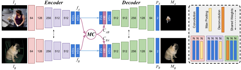
Figure 2: Deep Object Co-Segmentation. Our network includes three parts: (i) passing input images $I_{A}$ and $I_{B}$ through a Siamese encoder to extract feature maps $f_{A}$ and $f_{B}$, (ii) using a mutual correlation network to perform feature matching to obtain correspondence maps $C_{AB}$ and $C_{BA}$, (iii) passing concatenation of squeezed feature maps and correspondence maps through a Siamese decoder to get the common objects masks $M_{A}$ and $M_{B}$.

3 Method

In this section, we introduce a new CNN architecture for segmenting the common objects from two input images. The architecture is end-to-end trainable for the object co-segmentation task. Fig. 2 illustrates the overall structure of our architecture. Our network consists of three main parts: (1) Given two input images $I_{A}$ and $I_{B}$, we use a Siamese encoder to extract high-level semantic feature maps $f_{A}$ and $f_{B}$. (2) Then, we propose a mutual correlation layer to obtain correspondence maps $C_{AB}$ and $C_{BA}$ by matching feature maps $f_{A}$ and $f_{B}$ at pixel-level. (3) Finally, given the concatenation of the feature maps $f_{A}$ and $f_{B}$ and correspondence maps $C_{AB}$ and $C_{BA}$, a Siamese decoder is used to obtain and refine the common object masks $M_{A}$ and $M_{B}$.

In the following, we first describe each of the three parts of our architecture in detail. Then in Sec 3.4, the loss function is introduced. Finally, in Sec 3.5, we explain how to extend our approach to handle co-segmentation of a group of images, i.e. going beyond two images.

3.1 Siamese Encoder

The first part of our architecture is a Siamese encoder which consists of two identical feature extraction CNNs with shared parameters. We pass the input image pair $I_{A}$ and $I_{B}$ through the Siamese encoder network pair to extract feature maps $f_{A}$ and $f_{B}$. More specifically, our encoder is based on the VGG16 network [35]. We keep the first 13 convolutional layers and replace fc6 and fc7 with two $3\times 3$ convolutional layers conv6-1 and conv6-2 to produce feature maps which contain more spatial information. In total, our encoder network has 15 convolutional layers and 5 pooling layers to create a set of high-level semantic features $f_{A}$ and $f_{B}$. The input to the Siamese encoder is two $512\times 512$ images and the output of the encoder is two $1024$-channel feature maps with a spatial size of $16\times 16$.

3.2 Mutual Correlation

The second part of our architecture is a mutual correlation layer. The outputs of encoders $f_{A}$ and $f_{B}$ represent the high-level semantic content of the input images. When the two images contain objects that belong to a common class, they should contain similar features at the locations of the shared objects. Therefore, we propose a mutual correlation layer to compute the correlation between each pair of locations on the feature maps. The idea of utilizing the correlation layer is inspired by Flownet [10], in which the correlation layer is used to match feature points between frames for optical flow estimation. Our motivation of using the correlation layer is to filter the heat-maps (high-level features), which are generated separately for each input image, to highlight the heat-maps on the common objects (see Fig. 3).

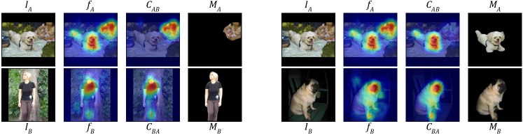
Figure 3: The visualization of the heat-maps. Given a pair of input images $I_{A}$ and $I_{B}$, after passing them through the Siamese encoder, we extract feature maps $f_{A}$ and $f_{B}$. We use the mutual correlation layer to perform feature matching to obtain correspondence maps $C_{AB}$ and $C_{BA}$. Then, using our Siamese decoder we predict the common objects masks $M_{A}$ and $M_{B}$. As shown before correlation layer, the heat-maps are covering all the objects inside the images. After applying the correlation layer, the heat-maps on uncommon objects are filtered out. Therefore, we utilize the output of the correlation layer to guide the network for segmenting the common objects.

In detail, the mutual correlation layer performs a pixel-wise comparison between two feature maps $f_{A}$ and $f_{B}$. Given a point $(i,j)$ and a point $(m,n)$ inside a patch around $(i,j)$, the correlation between feature vectors $f_{A}(i,j)$ and $f_{B}(m,n)$ is defined as

$$C_{AB}(i,j,k)=\langle\ f_{A}(i,j),f_{B}(m,n)\rangle$$ (1)

where $k=(n-j)D+(m-i)$ and $D\times D$ is patch size. Since the common objects can locate at any place on the two input images, we set the patch size to $D=2*max(w-1,h-1)+1$, where $w$ and $h$ are the width and height of the feature maps $f_{A}$ and $f_{B}$. The output of the correlation layer is a feature map $C_{AB}$ of size $w\times\ h\times D^{2}$. We use the same method to compute the correlation map $C_{BA}$ between $f_{B}$ and $f_{A}$.

3.3 Siamese Decoder

The Siamese decoder is the third part of our architecture, which predicts two foreground masks of the common objects. We squeeze the feature maps $f_{A}$ and $f_{B}$ and concatenate them with their correspondence maps $C_{AB}$ and $C_{BA}$ as the input to the Siamese decoder (Fig. 2). The same as the Siamese encoder, the decoder is also arranged in a Siamese structure with shared parameters. There are five blocks in our decoder, whereby each block has one deconvolutional layer and two convolutional layers. All the convolutional and deconvolutional layers in our Siamese decoder are followed by a ReLU activation function. By applying a Softmax function, the decoder produces two probability maps $p_{A}$ and $p_{B}$. Each probability map has two channels, background and foreground, with the same size as the input images.

3.4 Loss Function

We define our object co-segmentation as a binary image labeling problem and use the standard cross entropy loss function to train our network. The full loss score $\mathcal{L}_{AB}$ is then estimated by $\mathcal{L}_{AB}=\mathcal{L}_{A}+\mathcal{L}_{B},$ where the $\mathcal{L}_{A}$ and the $\mathcal{L}_{B}$ are cross-entropy loss functions for the image $A$ and the image $B$, respectively.

3.5 Group Co-Segmentation

Although our architecture is trained for image pairs, our method can handle a group of images. Given a set of $N$ images $\mathcal{I}=\left\{I_{1},...,I_{N}\right\}$, we pair each image with $K\leq N-1$ other images from $\mathcal{I}$. Then, we use our DOCS network to predict the probability maps for the pairs, $\mathcal{P}=\left\{p_{n}^{k}:1\leq n\leq N,1\leq k\leq K\right\}$, where $p_{n}^{k}$ is the predicted probability map for the $k$th pair of image $I_{n}$. Finally, we compute the final mask $M_{n}$ for image $I_{n}$ as

$$M_{n}(x,y)=\mathrm{median}\{p_{n}^{k}(x,y)\}>\sigma.$$ (2)

where $\sigma$ is the acceptance threshold. In this work, we set $\sigma=0.5$. We use the median to make our approach more robust to groups with outliers.

4 Experiments

4.1 Datasets

Training a CNN requires a lot of data. However, existing co-segmentation datasets are either too small or have a limited number of object classes. The MSRC dataset [34] was first introduced for supervised semantic segmentation, then a subset was used for object co-segmentation [39]. This subset of MSRC only has 7 groups of images and each group has 10 images. The iCoseg dataset, introduced in [2], consists of several groups of images and is widely used to evaluate co-segmentation methods. However, each group contains images of the same object instance or very similar objects from the same class. The Internet dataset [31] contains thousands of images obtained from the Internet using image retrieval techniques. However, it only has three object classes: car, horse and airplane, where images of each class are mixed with other noise objects. In [11], Faktor and Irani use PASCAL dataset for object co-segmentation. They separate the images into $20$ groups according to the object classes and assume that each group only has one object. However, this assumption is not common for natural images.

Inspired by [11], we create an object co-segmentation dataset by adapting the PASCAL dataset labeled by [13]. The original dataset consists of $20$ foreground object classes and one background class. It contains $8,498$ training and $2,857$ validation pixel-level labeled images. From the training images, we sampled $161,229$ pairs of images, which have common objects, as a new co-segmentation training set. We used PASCAL validation images to sample $42,831$ validation pairs and $40,303$ test pairs. Since our goal is to segment the common objects from the pair of images, we discard the object class labels and instead we label the common objects as foreground. Fig. 1(d) shows some examples of image pairs of our object co-segmentation dataset. In contrast to [11], our dataset consists of image pairs of one or more arbitrary common classes.

4.2 Implementation Details and Runtime

We use the Caffe framework [18] to design and train our network. We use our co-segmentation dataset for training. We did not use any images from the MSCR, Internet or iCoseg datasets to fine tune our model. The conv1-conv5 layers of our Siamese encoder (VGG-16 net [35]) are initialized with weights trained on the Imagenet dataset [8]. We train our network on one GPU for $100$K iterations using Adam solver [20]. We use small mini-batches of $10$ image pairs, a momentum of $0.9$, a learning rate of $1e-5$, and a weight decay of $0.0005$.

Our method can handle a large set of images in linear time complexity $\mathcal{O}(N)$. As mentioned in Sec. 3.5 in order to co-segment an image, we pair it with $K$ ($K\leq N-1$) other images. In our experiments, we used all possible pairs to make the evaluations comparable to other approaches. Although in this case our time complexity is quadratic $\mathcal{O}(N^{2})$, our method is significantly faster than others.

Number of images	Others time	Our time
$2$	$8$ minutes [19]	$0.1$ seconds
$30$	$4$ to $9$ hours [19]	$43.5$ seconds
$30$	$22.5$ minutes [40]	$43.5$ seconds
$418$ ($14$ categories, $\sim 30$ images per category)	$29.2$ hours [11]	$10.15$ minutes
$418$ ($14$ categories, $\sim 30$ images per category)	$8.5$ hours [17]	$10.15$ minutes

To show the influence of number of pairs $K$, we validate our method on the Internet dataset w.r.t. $K$ (Table 1). Each image is paired with $K$ random images from the set. As shown, we achieve state-of-the-art performance even with $K=10$. Therefore, the complexity of our approach is $\mathcal{O}(KN)=\mathcal{O}(N)$ which is linear with respect to the group size.

Table 1: Influence of number of pairs $K$.

Internet	K=10		K=20		K=99(all)
(N=100)	P	J	P	J	P	J
Car	93.93	82.89	93.91	82.85	93.90	82.81
Horse	92.31	69.12	92.35	69.17	92.45	69.44
Airplane	94.10	65.37	94.12	65.45	94.11	65.43
Average	93.45	72.46	93.46	72.49	93.49	72.56

4.3 Results

We report the performance of our approach on MSCR [34, 38], Internet [31], and iCoseg [2] datasets, as well as our own co-segmentation dataset.

4.3.1 Metrics.

For evaluating the co-segmentation performance, there are two common metrics. The first one is Precision, which is the percentage of correctly segmented pixels of both foreground and background masks. The second one is Jaccard, which is the intersection over union of the co-segmentation result and the ground truth foreground segmentation.

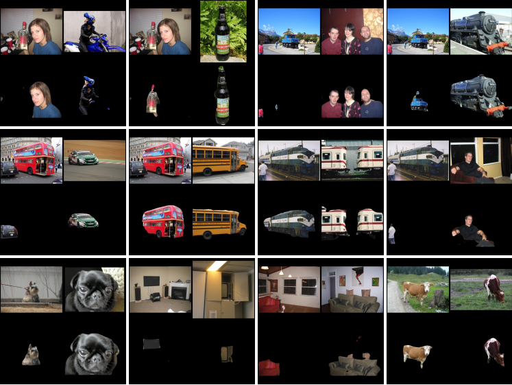
Figure 4: Our qualitative results on PASCAL Co-segmentation dataset. (odd rows) the input images, (even rows) the corresponding object co-segmentation results.

4.3.2 PASCAL Co-Segmentation.

As we mentioned in Sec 4.1, our co-segmentation dataset consists of $40,303$ test image pairs. We evaluate the performance of our method on our co-segmentation test data. We also tried to obtain the common objects of same classes using a deep semantic segmentation model, here FCN8s [25]. First, we train FCN8s with the PASCAL dataset. Then, we obtain the common objects from two images by predicting the semantic labels using FCN8s and keeping the segments with common classes as foreground. Our co-segmentation method (94.2% for Precision and 64.5% for Jaccard) outperforms FCN8s (93.2% for Precision and 55.2% for Jaccard), which uses the same VGG encoder, and trained with the same training images. The improvement is probably due to the fact that our DOCS architecture is specifically designed for the object co-segmentation task, which FCN8s is designed for the semantic labeling problem. Another potential reason is that generating image pairs is a form of data augmentation. We would like to exploit these ideas in the future work. Fig. 4 shows the qualitative results of our approach on the PASCAL co-segmentation dataset. We can see that our method successfully extracts different foreground objects for the left image when paired with a different image to the right.

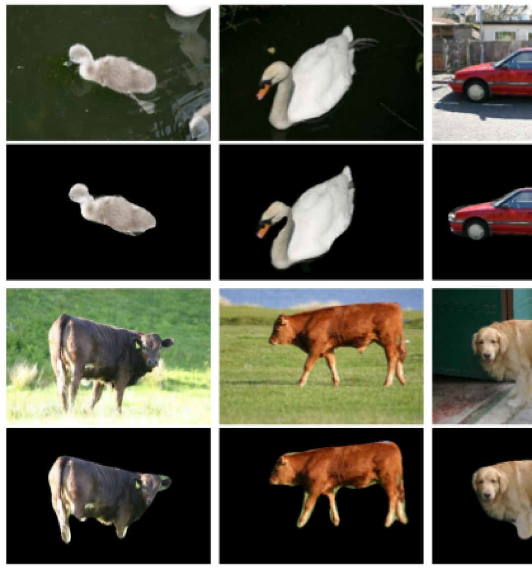
Figure 5: Our qualitative results on the MSRC dataset (seen classes). (odd rows) the input images, (even rows) the corresponding object co-segmentation results.

Table 2: Quantitative results on the MSRC dataset (seen classes). Quantitative comparison results of our DOCS approach with four state-of-the-art co-segmentation methods on the co-segmentation subset of the MSCR dataset.

MSCR	[39]	[31]	[40]	[11]	Ours
Precision	90.2	92.2	92.2	92.0	95.4
Jaccard	70.6	74.7	-	77.0	82.9

4.3.3 MSRC.

The MSRC subset has been used to evaluate the object co-segmentation performance by many previous methods [38, 31, 11, 40]. For the fair comparison, we use the same subset as [38]. We use our group co-segmentation method to extract the foreground masks for each group. In Table. 2, we show the quantitative results of our method as well as four state-of-the-art methods [39, 31, 11, 40]. Our Precision and Jaccard show a significant improvement compared to previous methods. It is important to note that [39] and [40] are supervised methods, i.e. both use images of the MSRC dataset to train their models. We obtain the new state-of-the-art results on this dataset even without training or fine-tuning on any images from the MSRC dataset. Visual examples of object co-segmentation results on the subset of the MSRC dataset can be found in Fig. 5.

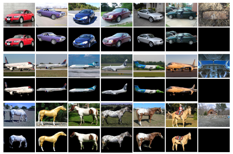
Figure 6: Our qualitative results on the Internet dataset (seen classes). (odd rows) the input images, (even rows) the corresponding object co-segmentation results.

Table 3: Quantitative results on the Internet dataset (seen classes). Quantitative comparison of our DOCS approach with several state-of-the-art co-segmentation methods on the co-segmentation subset of the Internet dataset. ‘P’ is the Precision, and ‘J’ is the Jaccard.

Internet		[19]	[31]	[6]	[28]	[45]	Ours
Car	P	58.7	85.3	87.6	88.5	90.4	93.9
	J	37.1	64.4	64.9	66.8	72.0	82.8
Horse	P	63.8	82.8	86.2	89.3	90.2	92.4
	J	30.1	51.6	33.4	58.1	65.0	69.4
Airplane	P	49.2	88.0	90.3	92.6	91.0	94.1
	J	15.3	55.8	40.3	56.3	66.0	65.4
Average	P	57.2	85.4	88.0	89.6	91.1	93.5
	J	27.5	57.3	46.2	60.4	67.7	72.6

4.3.4 Internet.

In our experiment, for the fair comparison, we followed [31, 6, 28, 45] to use the subset of the Internet dataset to evaluate our method. In this subset, there are 100 images in each category. We compare our method with five previous approaches [19, 6, 31, 28, 45]. Table 3 shows the quantitative results of each object category with respect to Precision and Jaccard. We outperform most of the previous methods [19, 6, 31, 28, 45] in terms of Precision and Jaccard. Note that [45] is a supervised co-segmentation method, [6] trained a discriminative Latent-SVM detector and [28] used a CNN trained on the ImageNet to extract semantic features. Fig. 6 shows some quantitative results of our method. It can be seen that even for the ‘noise’ images in each group, our method can successfully recognize them. We show the ‘noise’ images in the last column.

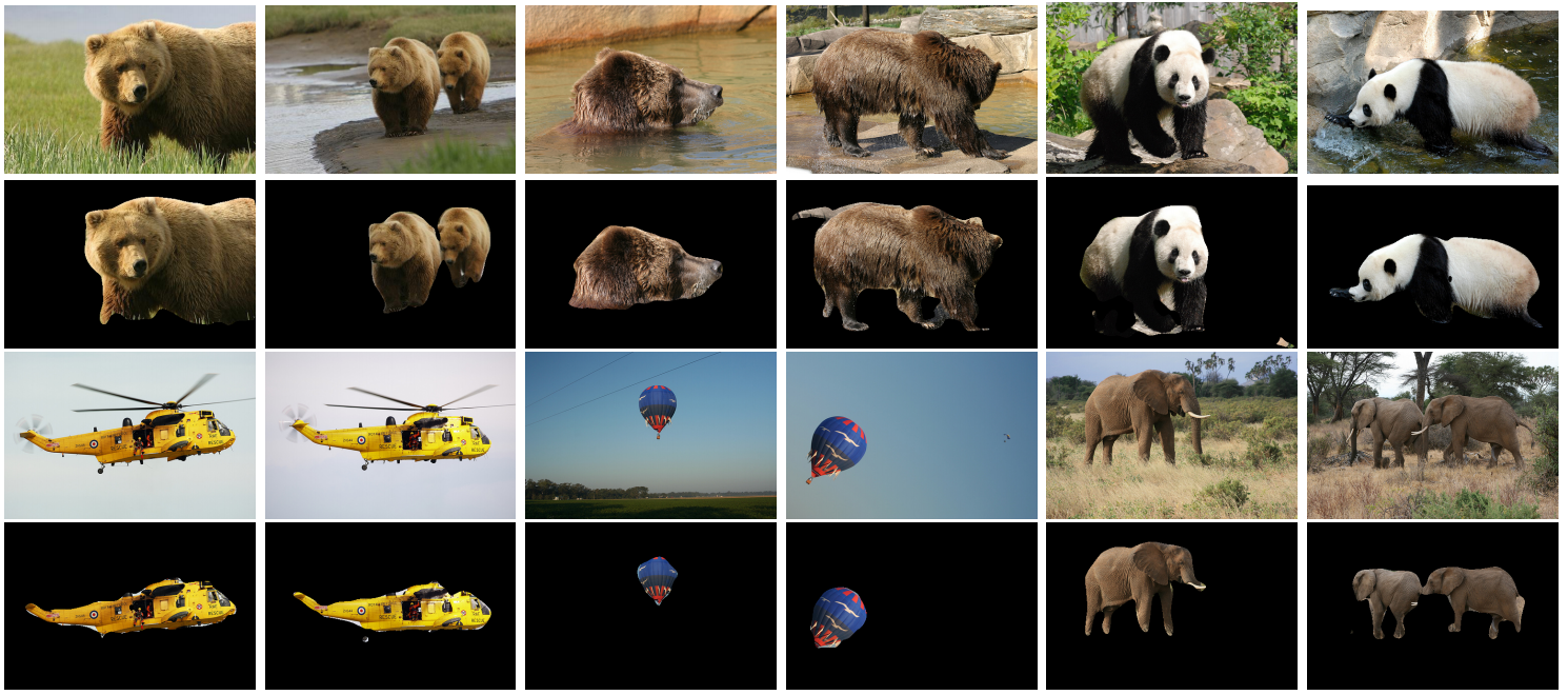
Figure 7: Our qualitative results on iCoseg dataset (unseen classes). Some results of our object co-segmentation method, with input image pairs in the odd rows and the corresponding object co-segmentation results in the even rows. For this dataset, the object classes were not known during training of our method (i.e. unseen).

Table 4: Quantitative results on the iCoseg dataset (unseen classes). Quantitative comparison of our DOCS approach with four state-of-the-art co-segmentation methods on some object classes of the iCoseg dataset, in terms of Jaccard. For this dataset, these object classes were not known during training of our method (i.e. unseen).

iCoseg	[31]	[16]	[11]	[17]	Ours
bear2	65.3	70.1	72.0	67.5	88.7
brownbear	73.6	66.2	92.0	72.5	91.5
cheetah	69.7	75.4	67.0	78.0	71.5
elephant	68.8	73.5	67.0	79.9	85.1
helicopter	80.3	76.6	82.0	80.0	73.1
hotballoon	65.7	76.3	88.0	80.2	91.1
panda1	75.9	80.6	70.0	72.2	87.5
panda2	62.5	71.8	55.0	61.4	84.7
average	70.2	73.8	78.2	74.0	84.2

4.3.5 iCoseg

To show that our method can generalize on unseen classes, i.e. classes which are not part of the training data, we need to evaluate our method on unseen classes. Batra et al. [2] introduced the iCoseg dataset for the interactive co-segmentation task. In contrast to the MSRC and Internet datasets, there are multiple object classes in the iCoseg dataset which do not appear in PASCAL VOC dataset. Therefore, it is possible to use the iCoseg dataset to evaluate the generalization of our method on unseen object classes. We choose eight groups of images from the iCoseg dataset as our unseen object classes, which are bear2, brown_bear, cheetah, elephant, helicopter, hotballoon, panda1 and panda2. There are two reasons for this choice: firstly, these object classes are not included in the PASCAL VOC dataset. Secondly, in order to focus on objects, in contrast to stuff, we ignore groups like pyramid, stonehenge and taj-mahal. We compare our method with four state-of-the-art approaches [16, 31, 11, 17] on unseen objects of the iCoseg dataset. Table 4 shows the comparison results of each unseen object groups in terms of Jaccard. The results show that for 5 out of 8 object groups our method performs best, and it is also superior on average. Note that the results of [16, 31, 11, 17] are taken from Table X in [17]. Fig. 7 shows some qualitative results of our method. It can be seen that our object co-segmentation method can detect and segment the common objects of these unseen classes accurately.

Furthermore to show the effect of number of PASCAL classes on the performance of our approach on unseen classes, we train our network on partial randomly picked PASCAL classes, i.e. $\{5,10,15\}$, and evaluate it on the iCoseg unseen classes. As it is shown in Table 5, our approach can generalize to unseen classes even when it is trained with only 10 classes from PASCAL.

Table 5: Analyzing the effect of number of training classes on unseen classes.

iCoseg	P(5)	P(10)	P(15)	P(20)
average	75.5	83.9	83.7	84.2

4.4 Ablation Study

To show the impact of the mutual correlation layer in our network architecture, we design a baseline network DOCS-Concat without using mutual correlation layers. In detail, we removed the correlation layer and we concatenate $f_{A}$ and $f_{B}$ (instead of $C_{AB}$) for image $I_{A}$ and concatenate $f_{B}$ and $f_{A}$ (instead of $C_{BA}$) for image $I_{B}$. In Table 6, we compare the performance of different network designs on multiple datasets. As shown, the mutual correlation layer in DOCS-Corr improved the performance significantly.

Table 6: Impact of mutual correlation layer.

	DOCS-Concat		DOCS-Corr
	Precision	Jaccard	Precision	Jaccard
Pascal VOC	92.6	49.9	94.2	64.5
MSRC	92.6	72.0	95.4	82.9
Internet	91.8	62.7	93.5	72.6
iCoseg(unseen)	93.6	78.9	95.1	84.2

5 Conclusions

In this work, we presented a new and efficient CNN-based method for solving the problem of object class co-segmentation, which consists of jointly detecting and segmenting objects belonging to a common semantic class from a pair of images. Based on a simple encoder-decoder architecture, combined with the mutual correlation layer for matching semantic features, we achieve state-of-the-art performance on various datasets, and demonstrate good generalization performance on segmenting objects of new semantic classes, unseen during training. To train our model, we compile a large object co-segmentation dataset consisting of image pairs from PASCAL dataset with shared objects masks.

Acknowledgements This work is funded by the DFG grant “COVMAP: Intelligente Karten mittels gemeinsamer GPS- und Videodatenanalyse” (RO 4804/2-1).

References

- [1] Badrinarayanan, V., Kendall, A., Cipolla, R.: Segnet: A deep convolutional encoder-decoder architecture for scene segmentation. TPAMI (2017)
- [2] Batra, D., Kowdle, A., Parikh, D., Luo, J., Chen, T.: icoseg: Interactive co-segmentation with intelligent scribble guidance. In: CVPR (2010)
- [3] Boykov, Y.Y., Jolly, M.P.: Interactive graph cuts for optimal boundary & region segmentation of objects in nd images. In: ICCV (2001)
- [4] Carreira, J., Sminchisescu, C.: Constrained parametric min-cuts for automatic object segmentation. In: CVPR (2010)
- [5] Chen, L.C., Papandreou, G., Kokkinos, I., Murphy, K., Yuille, A.L.: Semantic image segmentation with deep convolutional nets and fully connected crfs. In: ICLR (2015)
- [6] Chen, X., Shrivastava, A., Gupta, A.: Enriching visual knowledge bases via object discovery and segmentation. In: CVPR (2014)
- [7] Collins, M.D., Xu, J., Grady, L., Singh, V.: Random walks based multi-image segmentation: Quasiconvexity results and gpu-based solutions. In: CVPR (2012)
- [8] Deng, J., Dong, W., Socher, R., Li, L.J., Li, K., Fei-Fei, L.: Imagenet: A large-scale hierarchical image database. In: CVPR (2009)
- [9] Dong, X., Shen, J., Shao, L., Yang, M.H.: Interactive cosegmentation using global and local energy optimization. IEEE Transactions on Image Processing (2015)
- [10] Dosovitskiy, A., Fischer, P., Ilg, E., Hausser, P., Hazirbas, C., Golkov, V., van der Smagt, P., Cremers, D., Brox, T.: Flownet: Learning optical flow with convolutional networks. In: ICCV (2015)
- [11] Faktor, A., Irani, M.: Co-segmentation by composition. In: ICCV (2013)
- [12] Fu, H., Xu, D., Lin, S., Liu, J.: Object-based rgbd image co-segmentation with mutex constraint. In: CVPR (2015)
- [13] Hariharan, B., Arbelaez, P., Bourdev, L., Maji, S., Malik, J.: Semantic contours from inverse detectors. In: ICCV (2011)
- [14] Hochbaum, D.S., Singh, V.: An efficient algorithm for co-segmentation. In: ICCV (2009)
- [15] Jain, S.D., Xiong, B., Grauman, K.: Pixel objectness. arXiv:1701.05349 (2017)
- [16] Jerripothula, K.R., Cai, J., Meng, F., Yuan, J.: Automatic image co-segmentation using geometric mean saliency. In: ICIP (2014)
- [17] Jerripothula, K.R., Cai, J., Yuan, J.: Image co-segmentation via saliency co-fusion. IEEE Transactions on Multimedia (2016)
- [18] Jia, Y., Shelhamer, E., Donahue, J., Karayev, S., Long, J., Girshick, R., Guadarrama, S., Darrell, T.: Caffe: Convolutional architecture for fast feature embedding. In: ACM Multimedia (2014)
- [19] Joulin, A., Bach, F., Ponce, J.: Discriminative clustering for image co-segmentation. In: CVPR (2010)
- [20] Kingma, D., Ba, J.: Adam: A method for stochastic optimization. In: ICLR (2015)
- [21] Kowdle, A., Batra, D., Chen, W.C., Chen, T.: imodel: Interactive co-segmentation for object of interest 3d modeling. In: ECCV workshop (2010)
- [22] Lee, C., Jang, W.D., Sim, J.Y., Kim, C.S.: Multiple random walkers and their application to image cosegmentation. In: CVPR (2015)
- [23] Li, G., Yu, Y.: Deep contrast learning for salient object detection. In: CVPR (2016)
- [24] Lin, G., Milan, A., Shen, C., Reid, I.: Refinenet: Multi-path refinement networks for high-resolution semantic segmentation. In: CVPR (2017)
- [25] Long, J., Shelhamer, E., Darrell, T.: Fully convolutional networks for semantic segmentation. In: CVPR (2015)
- [26] Mukherjee, L., Singh, V., Dyer, C.R.: Half-integrality based algorithms for cosegmentation of images. In: CVPR (2009)
- [27] Noh, H., Hong, S., Han, B.: Learning deconvolution network for semantic segmentation. In: ICCV (2015)
- [28] Quan, R., Han, J., Zhang, D., Nie, F.: Object co-segmentation via graph optimized-flexible manifold ranking. In: CVPR (2016)
- [29] Ronneberger, O., Fischer, P., Brox, T.: U-net: Convolutional networks for biomedical image segmentation. In: MICCAI (2015)
- [30] Rother, C., Minka, T., Blake, A., Kolmogorov, V.: Cosegmentation of image pairs by histogram matching-incorporating a global constraint into mrfs. In: CVPR (2006)
- [31] Rubinstein, M., Joulin, A., Kopf, J., Liu, C.: Unsupervised joint object discovery and segmentation in internet images. In: CVPR (2013)
- [32] Rubio, J.C., Serrat, J., López, A., Paragios, N.: Unsupervised co-segmentation through region matching. In: CVPR (2012)
- [33] Shen, T., Lin, G., Liu, L., Shen, C., Reid, I.: Weakly supervised semantic segmentation based on co-segmentation. In: BMVC (2017)
- [34] Shotton, J., Winn, J., Rother, C., Criminisi, A.: Textonboost: Joint appearance, shape and context modeling for multi-class object recognition and segmentation. In: ECCV (2006)
- [35] Simonyan, K., Zisserman, A.: Very deep convolutional networks for large-scale image recognition. In: ICLR (2015)
- [36] Taniai, T., Sinha, S.N., Sato, Y.: Joint recovery of dense correspondence and cosegmentation in two images. In: CVPR (2016)
- [37] Uijlings, J.R., Van De Sande, K.E., Gevers, T., Smeulders, A.W.: Selective search for object recognition. IJCV (2013)
- [38] Vicente, S., Kolmogorov, V., Rother, C.: Cosegmentation revisited: Models and optimization. In: ECCV (2010)
- [39] Vicente, S., Rother, C., Kolmogorov, V.: Object cosegmentation. In: CVPR (2011)
- [40] Wang, F., Huang, Q., Guibas, L.J.: Image co-segmentation via consistent functional maps. In: ICCV (2013)
- [41] Wang, L., Wang, L., Lu, H., Zhang, P., Ruan, X.: Saliency detection with recurrent fully convolutional networks. In: ECCV (2016)
- [42] Xu, N., Price, B., Cohen, S., Yang, J., Huang, T.: Deep grabcut for object selection. In: BMVC (2017)
- [43] Xu, N., Price, B., Cohen, S., Yang, J., Huang, T.S.: Deep interactive object selection. In: CVPR (2016)
- [44] Yu, F., Koltun, V.: Multi-scale context aggregation by dilated convolutions. In: ICLR (2016)
- [45] Yuan, Z., Lu, T., Wu, Y.: Deep-dense conditional random fields for object co-segmentation. In: IJCAI (2017)
- [46] Zhao, H., Shi, J., Qi, X., Wang, X., Jia, J.: Pyramid scene parsing network. In: CVPR (2017)
- [47] Zheng, S., Jayasumana, S., Romera-Paredes, B., Vineet, V., Su, Z., Du, D., Huang, C., Torr, P.H.S.: Conditional random fields as recurrent neural networks. In: ICCV (2015)