Recipe for creating an arbitrary number of Floquet chiral edge states

Abstract

Floquet states of periodically driven systems could exhibit rich topological properties. Many of them are absent in their static counterparts. One such example is the chiral edge states in anomalous Floquet topological insulators, whose description requires a new topological invariant and a novel type of bulk-edge correspondence. In this work, we propose a prototypical quenched lattice model, whose two Floquet bands could exchange their Chern numbers periodically and alternatively via touching at quasienergies $0$ and $\pi$ under the change of a single system parameter. This process in principle allows the generation of as many Floquet chiral edge states as possible in a highly controllable manner. The quantized transmission of these edge states are extracted from the Floquet scattering matrix of the system. The flexibility in controlling the number of topological edge channels provided by our scheme could serve as a starting point for the engineering of robust Floquet transport devices.

I Introduction

Floquet states of matter emerge from systems that are modulated periodically in time ColdAtomFTP ; ColdAtomFTP2 ; PhotonFTP0 ; PhotonFTP1 ; PhotonFTP2 ; PhononFTP ; PhononFTP2 . They possess intriguing transport and topological properties DKRGong ; OkaPRB2009 ; LindnerNP2011 ; DahlhausPRB2011 ; KitagawaPRB2011 ; DerekPRL2012 ; HailongPRE2013 ; TongPRB2013 ; LeonPRL2013 ; CayssolRRL2013 ; ThakurathiRRB2013 ; DerekPRB2014 ; GrushinPRL2014 ; Wang2014 ; ZhouEPJB2014 ; TitumPRL2015 ; XiongPRB2016 ; DLossPRLPRB ; KR4 , many of which are characterized by new types of topological invariants, classification schemes and bulk-edge correspondence that goes beyond any time-independent descriptions KitagawaPRB2010 ; JiangPRL2011 ; KunduPRL2013 ; Bomantara2016 ; ZhaoErH2014 ; ReichlPRA2014 ; LeonPRB2014 ; AnomalousESPRX ; FulgaPRB2016 ; YapPRB2017 ; YapMajorana2017 ; ZhouPRB2016 ; AsbothSTF ; NathanNJP2015 ; ClassificationFTP1 ; ClassificationFTP2 .

One example is the anomalous chiral edge states in Floquet topological insulators AnomalousESPRX . These states could traverse the Floquet gap at $\pi$-quasienergy, connecting the top of the highest and the bottom of the lowest bulk bands in the Floquet quasienergy Brillouin zone. They are characterized by a topological winding number defined at a given quasienergy within the gap, which is obtained by integrating both quasimomenta over the system’s Brillouin zone and time over a driving period. With these anomalous edge states, the difference of winding numbers in the gaps above and below a Floquet band gives its Chern number, but the summation of Chern numbers below a Floquet gap cannot tell the number of chiral edge states traversing it from bottom to top. This leads to the identification of a new bulk-edge relation unique to Floquet systems AnomalousESPRX . The anomalous chiral edge states have also been used to achieve quantized non-adiabatic pumping in both clean and disordered samples AnomalousESPRX ; ZhouPRB2016 .

To date, anomalous Floquet chiral edge states have been observed in photonic PhotonFTP2 and acoustic PhononFTP2 systems. However, the experimentally realized models support only a single pair of chiral edge states in each gap, limiting its potential in the study of possible Floquet phases with many chiral edge states and large winding numbers. Floquet topological phases with many chiral edge states could not only admit rich topological structures DerekPRL2012 ; ZhouEPJB2014 ; DerekPRB2014 ; XiongPRB2016 , but also be useful in realizing Floquet transport devices with a large number of topologically protected channels along the edge YapPRB2017 ; YapMajorana2017 . In this work, we propose a simple scheme to generate any given number of chiral edge states in a Floquet system, and demonstrate our scheme in a prototypical quenched lattice model. The two-terminal transport of the model is also studied using the Floquet scattering matrix approach.

II Recipe for creating many chiral edge states

In this section, we introduce our Floquet engineering scheme, which in principle allows the generation of arbitrarily many chiral edge states in a well-controlled manner. An illustration of the process is shown in Fig. 1. For simplicity, we consider a two-band insulator with band Chern numbers $\pm 1$, and assume that under the increase of a system parameter, the two bands exchange their Chern numbers every time when they touch with each other and re-separate.

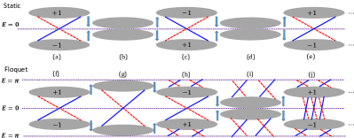
Figure 1: (color online) The scheme of generating many chiral edge states by periodically exchanging Floquet band Chern numbers, alternatively via band touchings at $0$ and $\pi$ quasienergies under the change of a system parameter (from left to right in each case). For demonstration purpose, a two-band Floquet system is presented, whereas the scheme is also applicable to multiple-band systems. In both cases, shaded regions represent bulk bands, and blue solid (red dashed) lines denote states localized around the left (right) edge of the lattice. Panels (a-e) represent the process in a static system: after two permutations of Chern numbers via band touchings, the system goes back to its initial topological phase and no new chiral edge states appear. Panels (f-j) illustrate the process in a Floquet system: after two permutations of band Chern numbers, alternatively at $\pi$ and $0$ quasienergies via band touchings, the system reaches a new topological phase with the same Chern number as before but possessing more chiral edge states traversing both Floquet gaps around $0$ and $\pi$ quasienergies.

It is instructive to compare the situations in a static and a Floquet system. In a static system, the two bands (shaded areas in Fig. 1) can only touch by closing the gap around energy $E=0$, as shown in Fig. 1(b). Due to the bulk-edge correspondence, the two chiral edge bands denoted by blue solid and red dashed lines in Fig. 1(a) will exchange their chiralities after the gap reopens around $E=0$ as shown in Fig. 1(c), whereas the net number of chiral edge states in the gap does not change during the transition. After a second topological phase transition, in which the two bands exchange their Chern numbers again [Fig. 1(d)], the system will go back to its initial topological phase with the same number of chiral edge states [Fig. 1(e)], and the story ends here.

The situation in a Floquet system, however, can be much richer. Due to the periodicity of Floquet quasienergy $E$, a two-band Floquet insulator has two gaps at $0$- and $\pi$-quasienergies. Therefore, the two Floquet bands can exchange their Chern numbers by touching at either quasienergy $0$ or $\pi$. Now if the increase of a system parameter could result in the closure of Floquet gaps at quasienergies $0$ and $\pi$ periodically and alternatively, more and more chiral edges should emerge in both gaps in order to compensate for the exchange of Floquet band Chern numbers during each topological phase transitions.

One example of such a process is sketched in Fig. 1(f-j) (with the increase of a system parameter from left to right panels). At the starting point [Fig. 1(f)], we have a Floquet insulator with bulk Chern numbers $\pm 1$ and two chiral edge bands crossing the Floquet gap at quasienergy $0$. With the increase of a system parameter, the two bulk bands gradually shift upward and downward, respectively, until exchanging their Chern numbers upon touching at quasienergy $\pi$ [Fig. 1(g)]. But since the number of chiral edge states at quasienergy $0$ cannot change during this process, two extra pairs of anomalous chiral edge bands crossing the $\pi$-quasienergy gap must appear after the transition. The resulting band structure is shown in Fig. 1(h), where we have one pair (two pairs) of normal (anomalous) chiral edge bands in the $0$-($\pi$-) quasienergy gap. With further increasing of the system parameter, the two bands “kiss” again and exchange their Chern numbers at quasienergy $0$ [Fig. 1(i)]. This time, the number of anomalous chiral edge states at quasienergy $\pi$ cannot change, and therefore the number of chiral edge bands crossing quasienergy $0$ must increase by $2$ after the transition. The resulting Floquet band structure is shown in Fig. 1(j). Though sharing the same Chern numbers with the initial topological phase [Fig. 1(f)], the final system possesses two more pairs of chiral edge bands in both $0$- and $\pi$-quasienergy gaps, and therefore should be characterized by larger topological winding numbers AnomalousESPRX . It is not hard to image that if this process could continue periodically with the increase of the system parameter, we would in principle reach a topological phase with arbitrarily large winding numbers, and therefore obtaining as many chiral edge states as possible in both Floquet gaps.

The question is how complicated a system should be to realize such an intriguing process. In the following section, we will introduce a periodically quenched two-dimensional ($2$d) lattice model with only nearest neighbor hoppings. It will be shown that this simple model realizes exactly the sequence of topological phase transitions described in this section, which is accompanied by a monotonic increasing of the number of Floquet chiral edge states under the increase of just a single hopping parameter of the lattice.

III Prototypical model: a periodically quenched lattice

Our model contains noninteracting particles in a $2$d square lattice, with $2$ degrees of freedom (sublattice or spin) in each unit cell. The nearest neighbor (NN) hopping amplitude and onsite potential of the lattice are periodically modulated in time. In each driving period, the system is subjected to a sequence of three quenches, as sketched in Fig. 2. The dynamics of the system following each quench is described by the Schrodinger equation $i\frac{d}{dt}|\psi(t)\rangle=\hat{{\cal H}}|\psi(t)\rangle$, with the Hamiltonian

$$\hat{{\cal H}}=\hat{{\cal H}}_{1}=\frac{3J_{1}}{2i}\sum_{n_{x},n_{y}}(|n_{x},n_{y}\rangle\langle n_{x}+1,n_{y}|-{\rm h.c.})\otimes\sigma_{x}$$ (1)

for $t\in\left[\ell,\ell+\frac{1}{3}\right)$,

$$\hat{{\cal H}}=\hat{{\cal H}}_{2}=\frac{3J_{2}}{2i}\sum_{n_{x},n_{y}}(|n_{x},n_{y}\rangle\langle n_{x},n_{y}+1|-{\rm h.c.})\otimes\sigma_{y}$$ (2)

for $t\in\left[\ell+\frac{1}{3},\ell+\frac{2}{3}\right)$, and

$$\hat{{\cal H}}=\hat{{\cal H}}_{3}= \frac{3J_{3}}{2}\sum_{n_{x},n_{y}}(M|n_{x},n_{y}\rangle\langle n_{x},n_{y}|$$ (3)

$$+ |n_{x},n_{y}\rangle\langle n_{x}+1,n_{y}|+|n_{x},n_{y}\rangle\langle n_{x},n_{y}+1|+{\rm h.c.})\otimes\sigma_{z}$$

for $t\in\left[\ell+\frac{2}{3},\ell+1\right)$, where $n_{x},n_{y},\ell$ are integers and $\sigma_{x,y,z}$ are Pauli matrices. In this manuscript we set the Planck constant, driving period, and lattice constant all equal to $1$.

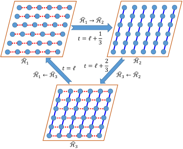
Figure 2: (color online) A sketch of the quenched lattice model in the $\ell$’s driving period. The same sequence of quenches is applied to the lattice for every driving period $\ell\in\mathbb{Z}$. Each shaded dot represents a unit cell with two internal degrees of freedom (sublattice or spin). At $t=\ell$, the system Hamiltonian is quenched to $\hat{{\cal H}}_{1}$, for which there are only NN hoppings (red dashed lines) along $x$ (horizontal) direction of the lattice. At $t=\ell+\frac{1}{3}$, the system Hamiltonian is switched to $\hat{{\cal H}}_{2}$, for which there are only NN hoppings (blue solid lines) along $y$ (vertical) direction of the lattice. At $t=\ell+\frac{2}{3}$, the system’s Hamiltonian is quenched to $\hat{{\cal H}}_{3}$, for which NN hoppings along both $x$ and $y$ directions of the lattice are switched on, and an energy bias between two internal degrees of freedom is applied within each unit cell.

In the first one third of a driving period, the system is described by the Hamiltonian $\hat{{\cal H}}_{1}$, where there are only NN hoppings along $x$-direction of the lattice with a hopping amplitude $\frac{3J_{1}}{2}$. In the second one third of a driving period, the system Hamiltonian is switched to $\hat{{\cal H}}_{2}$, where there are only NN hoppings along $y$-direction of the lattice with a hopping amplitude $\frac{3J_{2}}{2}$. Finally, in the last one third of a driving period, the system Hamiltonian is quenched to $\hat{{\cal H}}_{3}$, where there are NN hoppings along both $x$ and $y$ directions with equal hopping amplitudes $\frac{3J_{3}}{2}$, together with an onsite potential $\frac{3J_{3}M}{2}$. Putting together, the Floquet operator generating the evolution of the system over a complete driving period is given by $\hat{U}=e^{-i\frac{1}{3}\hat{{\cal H}}_{3}}e^{-i\frac{1}{3}\hat{{\cal H}}_{2}}e^{-i\frac{1}{3}\hat{{\cal H}}_{1}}$. To simplify the notation, we introduce an “effective” Hamiltonian for each step of quenched evolutions as $\hat{H}_{i}=\frac{1}{3}\hat{{\cal H}}_{i}$ ($i=1,2,3$). Then the system we are going to study is described by the Floquet operator

$$\hat{U}=e^{-i\hat{H}_{3}}e^{-i\hat{H}_{2}}e^{-i\hat{H}_{1}}.$$ (4)

Since only NN couplings in the lattice are required in each step of the quench, our model should be in principle realizable in photonic setups like those reported in Ref. PhotonFTP2 . In the following section, we will study the bulk Floquet quasienergy spectrum and Chern numbers of $\hat{U}$ at different hopping parameters $J_{1}$ or $J_{2}$. We will further demonstrate that by increasing the value of $J_{1}$ or $J_{2}$, a sequence of topological phase transitions can be induced, in which the two Floquet bands of $\hat{U}$ exchange their Chern numbers alternatively upon touching at quasienergies $0$ and $\pi$, realizing the scheme we described in Sec. II.

IV Bulk spectrum and Chern number

In this section, we study the bulk Floquet spectrum and Chern numbers of our periodically quenched lattice model. For a lattice with $N_{x}\times N_{y}$ unit cells and under periodic boundary conditions (PBC) along both $x$ and $y$ directions, we can perform a Fourier transform $|k_{x},k_{y}\rangle=\frac{1}{\sqrt{N_{x}N_{y}}}\sum_{n_{x}=1}^{N_{x}}\sum_{n_{y}=1}^{N_{y}}e^{i(k_{x}n_{x}+k_{y}n_{y})}|n_{x},n_{y}\rangle$ to find the Floquet operator as $\hat{U}=\sum_{k_{x},k_{y}}|k_{x},k_{y}\rangle U(k_{x},k_{y})\langle k_{x},k_{y}|$, where $k_{x,y}\in[0,2\pi)$ are two quasimomenta. The Bloch-Floquet operator $U(k_{x},k_{y})$ has the form

$$U(k_{x},k_{y})=e^{-iH_{3}(k_{x},k_{y})}e^{-iH_{2}(k_{y})}e^{-iH_{1}(k_{x})},$$ (5)

with Bloch Hamiltonians

$$H_{1}(k_{x})= \,J_{1}\sin(k_{x})\sigma_{x}\equiv{\cal K}_{1}\sigma_{x},$$ (6)

$$H_{2}(k_{y})= \,J_{2}\sin(k_{y})\sigma_{y}\equiv{\cal K}_{2}\sigma_{y},$$ (7)

$$H_{3}(k_{x},k_{y})= \,J_{3}[M+\cos(k_{x})+\cos(k_{y})]\sigma_{z}\equiv{\cal K}_{3}\sigma_{z}.$$ (8)

Note in passing that in the static limit, $H_{1}(k_{x})+H_{2}(k_{y})+H_{3}(k_{x},k_{y})$ describes the paradigmatic Qi-Wu-Zhang (QWZ) model of Chern insulators QWZ . The QWZ model possesses two topologically nontrivial phases in the range of $M\in(-2,2)$, separated by a phase transition at $M=0$. In each of these topological nontrivial phases, there is only a single pair of chiral edge states traversing the band gap. As will be shown, our simple quench protocol endowed the QWZ model with much richer topological phase structures that are unique to Floquet systems.

To see this, let us first check the Floquet spectrum of $U(k_{x},k_{y})$, which is obtained by solving the eigenvalue equation $U(k_{x},k_{y})|\psi\rangle=e^{-iE(k_{x},k_{y})}|\psi\rangle$. It is directly seen that the quasienergies (eigenphases) of $U(k_{x},k_{y})$ group into two Floquet bands with dispersions

$$E_{\pm}(k_{x},k_{y})= \pm|\arccos[\cos({\cal K}_{3})\cos({\cal K}_{2})\cos({\cal K}_{1})$$

$$+ \sin({\cal K}_{3})\sin({\cal K}_{2})\sin({\cal K}_{1})]|.$$ (9)

In general, there are two spectrum gaps at quasienergies $0$ and $\pi$. We characterize them by the gap functions:

$$\Delta_{0}= \min_{\{k_{x},k_{y}\}}2|E_{\pm}(k_{x},k_{y})|,$$ (10)

$$\Delta_{\pi}= \min_{\{k_{x},k_{y}\}}2[\pi-|E_{\pm}(k_{x},k_{y})|].$$ (11)

So the spectrum gap closes at quasienergy $0$ ($\pi$) if $\Delta_{0}=0$ ($\Delta_{\pi}=0$). In Fig. 3(a), we plot $\Delta_{0}$ (blue dashed line) and $\Delta_{\pi}$ (red solid line) versus $J_{2}$ at fixed values of $J_{1}=0.5\pi$, $J_{3}=0.2\pi$ and $M=1$. We observe that the bulk quasienergy dispersions $E_{\pm}(k_{x},k_{y})$ become gapless every time when $J_{2}$ hits an integer multiple of $\pi$. Furthermore, the following pattern of gap closing conditions are identified:

$$J_{2}=\begin{cases}2n\pi,&\Delta_{0}=0\\ (2n+1)\pi,&\Delta_{\pi}=0\end{cases}\qquad n=0,1,2,....$$ (12)

That is, the spectrum gap closes alternatively at quasienergies $0$ and $\pi$ with the increase of $J_{2}$. Similar behaviors of $\Delta_{0}$ and $\Delta_{\pi}$ versus $J_{1}$ are also found at fixed values of the other parameters. Also we note that the maximal size of spectrum gaps at both quasienergies $0$ and $\pi$ is maintained under the increase of either $J_{1}$ or $J_{2}$.

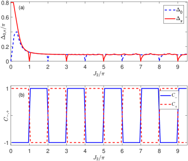
Figure 3: (color online) Floquet spectrum gaps and Chern numbers versus the hopping amplitude $J_{2}$ at fixed values of $(J_{1},J_{3},M)=(0.5\pi,0.2\pi,1)$. Panel (a): gaps at quasienergies $0$ (blue dashed line) and $\pi$ (red solid line) as defined in Eqs. (10) and (11), respectively. Panel (b): Chern numbers $C_{-}$ (blue solid line) and $C_{+}$ (red dashed line) of the lower and higher Floquet bands $E_{-}$ and $E_{+}$, respectively.

As discussed in Sec. II, in order for such a gap evolution process to generate large winding numbers in both the $0$- and $\pi$-quasienergy gaps, the two Floquet bands need to exchange their Chern numbers every time when they touch with each other. To check this, we compute the Floquet band Chern numbers $C_{\pm}$ of $U(k_{x},k_{y})$ versus $J_{2}$ at fixed values of $J_{1}=0.5\pi$, $J_{3}=0.2\pi$ and $M=1$. The Chern number of the Floquet band below (above) quasienergy $0$ is denoted by the blue solid (red dashed) line in Fig. 3(b). We see that the two bands indeed exchange their Chern numbers every time when $J_{2}$ passes through an integer $(n)$ multiple of $\pi$, where the gap closes at ($0$-) $\pi$-quasienergy if $n$ is even (odd). Furthermore, this process happens periodically under the increasing of $J_{2}$. A similar process is also observed under the increasing of $J_{1}$ with other system parameters fixed. Putting together, the quenched lattice model described by Floquet operator (4) indeed exemplifies the scheme of generating large gap winding numbers and chiral edge states as we proposed in Sec. II. In the following section, we will illustrate this point more explicitly by investigating the spectrum of $\hat{U}$ under open boundary conditions and discussing its bulk-edge correspondence.

V Chiral edge states

According to the bulk-edge correspondence of $2$d Floquet insulators AnomalousESPRX , the Chern number $C_{\alpha}$ of a bulk Floquet band $\alpha$ can be expressed as

$$C_{\alpha}=W_{E}[\hat{U}]-W_{E^{\prime}}[\hat{U}],$$ (13)

where $W_{E}$ ($W_{E^{\prime}}$) is the winding number of the system’s Floquet operator $\hat{U}$ at quasienergy $E$ ($E^{\prime}$) in the quasienergy gap above (below) the band $\alpha$. Furthermore, under PBC along one dimension of the $2$d lattice and OBC along the other, the number of chiral edge states localized around one edge of the lattice $n_{{\rm edge}}(E)$ with a quasienergy $E$ in the gap is related to the winding number as AnomalousESPRX

$$n_{{\rm edge}}(E)=|W_{E}[\hat{U}]|.$$ (14)

Since a two-band Floquet insulator has two gaps at quasienergies $0$ and $\pi$, the bulk-edge relations (13, 14) make it possible for the system to have small bulk Chern numbers $C_{\pm}$ but large winding numbers $(W_{0},W_{\pi})$, and therefore many chiral edge states traversing both of the quasienergy gaps.

The model we introduced in Sec. III belongs exactly to this situation. To be explicit, we compute the Floquet spectrum of $\hat{U}$ under a mixed boundary condition (MBC), for which we denote the case with OBC/PBC along $x$-direction and PBC/OBC along $y$-direction of the lattice as MBCX/MBCY. The Floquet operator under MBCX is denoted by $\hat{U}(k_{y})=e^{-i\hat{H}_{3}(k_{y})}e^{-i\hat{H}_{2}(k_{y})}e^{-i\hat{H}_{1}}$, where

$$H_{1}= \,\frac{J_{1}}{2i}\sum_{n_{x}=1}^{N_{x}-1}(|n_{x}\rangle\langle n_{x}+1|-{\rm h.c.})\otimes\sigma_{x},$$ (15)

$$H_{2}(k_{y})= \,J_{2}\sin(k_{y})\sum_{n_{x}=1}^{N_{x}}|n_{x}\rangle\langle n_{x}|\otimes\sigma_{y},$$ (16)

$$H_{3}(k_{y})= \,J_{3}[M+\cos(k_{y})]\sum_{n_{x}=1}^{N_{x}}|n_{x}\rangle\langle n_{x}|\otimes\sigma_{z}$$

$$+ \,\frac{J_{3}}{2}\sum_{n_{x}=1}^{N_{x}-1}(|n_{x}\rangle\langle n_{x}+1|+{\rm h.c.})\otimes\sigma_{z}.$$ (17)

Similarly, the Floquet operator under MBCY is denoted by $\hat{U}(k_{x})=e^{-i\hat{H}_{3}(k_{x})}e^{-i\hat{H}_{2}}e^{-i\hat{H}_{1}(k_{x})}$, with

$$H_{1}(k_{x})= \,J_{1}\sin(k_{x})\sum_{n_{y}=1}^{N_{y}}|n_{y}\rangle\langle n_{y}|\otimes\sigma_{x},$$ (18)

$$H_{2}= \,\frac{J_{2}}{2i}\sum_{n_{y}=1}^{N_{y}-1}(|n_{y}\rangle\langle n_{y}+1|-{\rm h.c.})\otimes\sigma_{y},$$ (19)

$$H_{3}(k_{x})= \,J_{3}[M+\cos(k_{x})]\sum_{n_{y}=1}^{N_{y}}|n_{y}\rangle\langle n_{y}|\otimes\sigma_{z}$$

$$+ \,\frac{J_{3}}{2}\sum_{n_{y}=1}^{N_{y}-1}(|n_{y}\rangle\langle n_{y}+1|+{\rm h.c.})\otimes\sigma_{z}.$$ (20)

The quasienergy dispersions of $\hat{U}(k_{y})$ and $\hat{U}(k_{x})$ at several different values of $J_{2}$ are shown in Figs. 4 and 5, with the number of unit cells $N_{x}=200$ and $N_{y}=200$ for the two cases, respectively. In all the panels, gray regions represent bulk Floquet bands and blue solid (red dashed) lines denote chiral edge states localized around the left (right) boundary of the lattice. The Chern numbers $C_{\pm}$ of bulk Floquet bands and winding numbers $W_{0,\pi}$ of chiral edge states at quasienergies $0$ and $\pi$ are also denoted in the figure. The other system parameters are set at $(J_{1},J_{3},M)=(0.5\pi,0.2\pi,1)$ for all the calculations.

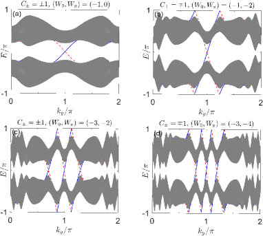
Figure 4: (color online) The Floquet spectrum of $\hat{U}(k_{y})$ under OBC and PBC along $x$ and $y$ directions of the lattice, respectively. Gray regions represent bulk bands. Blue solid (red dashed) lines refer to edge states localized at the left (right) edge of the lattice. The lattice has $N_{x}=200$ unit cells along $x$ direction. The hopping amplitude $J_{2}$ take values as (a) $J_{2}=0.5\pi$, (b) $J_{2}=1.5\pi$, (c) $J_{2}=2.5\pi$ and (d) $J_{2}=3.5\pi$. Other system parameters are set at $(J_{1},J_{3},M)=(0.5\pi,0.2\pi,1)$. $C_{-}$ ($C_{+}$) is the Chern numbers of the lower (upper) Floquet band and $W_{0}$ ($W_{\pi}$) is the edge state winding number at quasienergy $0$ ($\pi$).

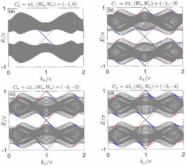
Figure 5: (color online) The Floquet spectrum of $\hat{U}(k_{x})$ under OBC and PBC along $y$ and $x$ directions of the lattice, respectively. Gray regions represent bulk bands. Blue solid (red dashed) lines refer to edge states localized at the left (right) edge of the lattice. The lattice has $N_{y}=200$ unit cells along $y$ direction. The hopping amplitude $J_{2}$ take values as (a) $J_{2}=0.5\pi$, (b) $J_{2}=1.5\pi$, (c) $J_{2}=2.5\pi$ and (d) $J_{2}=3.5\pi$. Other system parameters are set at $(J_{1},J_{3},M)=(0.5\pi,0.2\pi,1)$. $C_{-}$ ($C_{+}$) is the Chern numbers of the lower (upper) Floquet band and $W_{0}$ ($W_{\pi}$) is the edge state winding number at quasienergy $0$ ($\pi$).

In both Figs. 4 and 5, we see that two more pairs of chiral edge states emerge every time when the value of $J_{2}$ increases by $\pi$. If the gap closes at quasienergy $0$ ($\pi$) during this process, these new edge states will appear in the gap centered at quasienergy $0$ ($\pi$) after the transition. Furthermore, for a given $J_{2}$, the number of chiral edge states in each gap is the same for both $\hat{U}(k_{y})$ and $\hat{U}(k_{x})$, indicating that these edge states are insensitive to the configuration of boundary conditions. More generally, under the chosen set of parameters $(J_{1},J_{3},M)=(0.5\pi,0.2\pi,1)$, we can infer the following pattern of edge state winding numbers $W_{0,\pi}$ at quasienergies $0$ and $\pi$:

$$W_{0}= -2n-1\quad{\rm for}\quad 2n\pi<J_{2}<(2n+2)\pi,$$ (21)

$$W_{\pi}= -2n\qquad\,\,\,{\rm for}\quad(2n-1)\pi<J_{2}<(2n+1)\pi,$$ (22)

where $n\in\mathbb{N}$ takes all possible nature numbers. Therefore, by tuning the value of hopping amplitude $J_{2}$, one can obtain in principle arbitrarily large winding numbers for both Floquet gaps centered around quasienergies $0$ and $\pi$. Then according to Eq. (14), arbitrarily many chiral edge states could appear in the gaps around quasienergies $0$ and $\pi$. An example of the spectrum with many chiral edge states is shown in Appendix A. By varying $J_{1}$ with other system parameters fixed, we observe a similar pattern for the winding numbers and edge states, with more details presented in Appendix B. Two other examples are discussed in Appendix C.

Note in passing that in Fig. 5, all the eigenstates at quasienergy $0$ or $\pi$ in each panel have the same quasimomentum $k_{x}=0$ and also almost the same group velocity $\partial_{k_{x}}E$. Then for a large enough sample in a large winding number phase, there will be a significant “synchronous” and “parallel” topological current flowing along its edge. Such a current might be more robust to perturbations and dephasing introduced by the environment, and therefore has the potential of realizing robust quantum information transfer.

In both static HighCN1 ; HighCN2 ; HighCN3 ; HighCN4 ; HighCN5 ; HighCN6 ; HighCN7 and Floquet DerekPRL2012 ; DerekPRB2014 ; ZhouEPJB2014 ; XiongPRB2016 ; YapPRB2017 $2$d topological insulators, efforts have been made to engineer bulk bands with large ($>1$) Chern numbers. An important aim is to find more chiral edge states, and therefore realizing more quantized and topologically protected transport channels along the sample edge YapPRB2017 ; YapMajorana2017 . However, many of the existing approaches require either more then $2$ bulk bands, or longer range hoppings plus a careful engineering of the local symmetry of the Brillouin zone. The scheme and quenched lattice model introduced in this manuscript go around most of these complications, and at the same time allow the generation of any requested number of chiral edge states in a well controlled manner. Our results could then serve as a starting point for both the theoretical exploration of rich Floquet topological phases in the regime of large winding numbers, and the practical design of Floquet devices with many quantized edge transport channels.

In the next section, we will demonstrate the transport of chiral edge states in our system by investigating their two-terminal conductance. The results show that both the normal and anomalous chiral edge states give quantized conductance, which are equal to their corresponding winding numbers.

VI Two-terminal conductance

In this section, we study the two-terminal transport of chiral edge states in our quenched lattice model using the approach of Floquet scattering matrix Scattering1 ; Scattering2 ; Scattering3 ; Scattering4 ; Scattering5 . The $2$d lattice is chosen to have a patch geometry with OBC along both $x$ and $y$ directions. The unit cell coordinates $n_{x}$ and $n_{y}$ take values in $1,2,...,N_{x}$ and $1,2,...,N_{y}$, respectively. Two absorbing leads are coupled to the quenched lattice at its left ($n_{x}=1$) and right ($n_{x}=N_{x}$) ends. These leads are assumed to act stroboscopically at the start and end of each Floquet driving period. In the lattice representation, their effects are described by the following projector onto leads Scattering4 ; Scattering5 :

$$P=\begin{bmatrix}\mathbb{I}_{N_{y}}&\mathbb{O}_{N_{y}\times(N_{x}-1)N_{y}}\\ \mathbb{O}_{N_{y}\times(N_{x}-1)N_{y}}&\mathbb{I}_{N_{y}}\end{bmatrix}\otimes\sigma_{0},$$ (23)

where $\mathbb{I}$ ($\mathbb{O}$) represents identity (zero) matrix and $\sigma_{0}$ is a $2\times 2$ identity corresponding to the internal degrees of freedom. Then for an incoming state with quasienergy $E$ from the left lead to the quenched lattice, we have a fancied scattering problem described by a quasienergy-dependent scattering matrix Scattering4 ; Scattering5 :

$$S(E)\equiv \begin{bmatrix}r(E)&t(E)\\ t^{\prime}(E)&r^{\prime}(E)\end{bmatrix}$$ (24)

$$= P\left[1-e^{iE}\hat{U}\left(1-P^{T}P\right)\right]^{-1}e^{iE}\hat{U}P^{T},$$ (25)

where the Floquet operator $\hat{U}$ is given by Eq. (4). Here the transmission amplitude $t(E)$ is a $2N_{y}$ by $2N_{y}$ matrix, from which the conductance of the quenched lattice (i.e., transmission from left to right leads) is obtained as $G(E)={\rm Tr}[t^{\dagger}(E)t(E)]$.

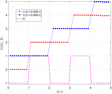
Figure 6: (color online) Two-terminal conductance $G(E)$ and Bott index $B_{-}$ of $\hat{U}$ versus the hopping amplitude $J_{2}$. Other system parameters are fixed at $(J_{1},J_{3},M)=(0.5\pi,0.2\pi,1)$ and the lattice size is $N_{x}=N_{y}=70$. Red triangles (blue dots) represent the transmission of an incoming state whose quasienergy $E$ is inside the Floquet spectrum gap centered around $E=\pi$ ($E=0$). The Bott index $B_{-}$ versus $J_{2}$ (magenta dashed line) follows the pattern of the lower band’s Chern number as shown in Fig. 1.

In Fig. 6. we present the calculation of $G(E)$ versus the hopping amplitude $J_{2}$ at fixed incoming quasienergies $E\approx 0$ (blue dots) and $E\approx\pi$ (red triangles). Referring to the Chern number pattern and Floquet spectrum presented in Figs. 3 and 4, we clearly see that $G(E)=n_{{\rm edge}}(E)$ for all values of $J_{2}$ studied here. This further verifies that the chiral edge states found in our system indeed give quantized conductances equaling to their winding numbers. For completeness, we also calculated the Bott index TitumPRL2015 ; Bott1 ; Bott2 ; Bott3 ; Bott4 ; Bott5 ; Bott6 of the lower Floquet band $B_{-}$ in our system (see Appendix D for the definition). For a filled Floquet band, the Bott index is equal to the Chern number, but it is also well-defined in a torus or patch geometry in position representation. Our results show that the change of $B_{-}$ versus $J_{2}$ (dashed line in Fig. 6) follows exactly the Chern number pattern of the lower band, but is unable to capture the winding number and the number of chiral edge states traversing a Floquet gap in our model. This suggests that the winding number introduced in Ref. AnomalousESPRX might be the most appropriate invariant to describe topological phases and phase transitions related to chiral edge states in $2$d Floquet insulators.

Note in passing that in a realistic two-terminal transport setting, an incoming state is prepared at certain energy instead of quasienergy. In this situation, the quantized edge state conductance is only recovered after applying a “Floquet sum rule” KunduPRL2013 , as also explored in Refs. YapPRB2017 ; YapMajorana2017 .

VII Summary

In this manuscript, we proposed a simple Floquet engineering recipe to generate many topological chiral edge states in a controlled manner. The essence of our approach is to let the Floquet bands of the system exchange their Chern numbers periodically and alternatively upon touching at $0$- and $\pi$-quasienergies. A prototypical quenched lattice model is introduced to demonstrate our idea. The quantized edge state conductance of the model in several different topological phases were obtained from the Floquet scattering matrix of the system. Our results reveal an intriguing mechanism in the engineering of Floquet transport devices.

In a realistic system, disorder could have important impacts on its topology and transport properties Disorder1 ; Disorder2 . The quenched lattice model proposed in this manuscript could be a promising platform to explore these effects. On the one hand, the phases with many topological chiral edge states in our system could be more robust to disorder effects, and potentially also more efficient in the realization of Floquet edge state pumps. On the other hand, topological phases with many chiral edge states are characterized by large winding numbers at both $0$- and $\pi$-quasienergy gaps. Exploring possible topological phase transitions induced by disorder in these large winding number phases is also an interesting topic for future study.

Appendix A Floquet spectrum of $\hat{U}$ with many chiral edge states: an example

In this appendix, we give an example of the Floquet spectrum of $\hat{U}$ defined in Eq. (4) of the main text with many chiral edge states traversing both the gaps around $0$ and $\pi$ quasienergies. The spectrum is shown in Fig. A.1, where $9$/$10$ pairs of chiral edge states are found in the spectrum gap centered around quasienergy $0/\pi$. For presentation purpose, only the range of spectrum in which edge states appear is shown.

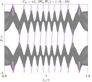
Figure A.1: (color online) The Floquet spectrum of $\hat{U}(k_{y})$ under OBC and PBC along $x$ and $y$ directions of the lattice, respectively. Shaded regions represent bulk bands. Blue crosses (red dots) refer to edge states localized at the left (right) edge of the lattice. The lattice has $N_{x}=300$ unit cells along $x$ direction. The hopping amplitude $J_{2}=9.5\pi$. Other system parameters are set at $(J_{1},J_{3},M)=(0.5\pi,0.2\pi,1)$. $C_{-}$ ($C_{+}$) is the Chern numbers of the lower (upper) Floquet band and $W_{0}$ ($W_{\pi}$) is the edge state winding number at quasienergy $0$ ($\pi$).

Appendix B Floquet spectrum of $\hat{U}$ at different values of $J_{1}$

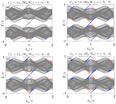
Figure B.1: (color online) The Floquet spectrum of $\hat{U}(k_{y})$ under OBC and PBC along $x$ and $y$ directions of the lattice, respectively. Gray regions represent bulk bands. Blue solid (red dashed) lines refer to edge states localized at the left (right) edge of the lattice. The lattice has $N_{x}=200$ unit cells along $x$ direction. The hopping amplitude $J_{1}$ take values as (a) $J_{1}=1.5\pi$, (b) $J_{1}=2.5\pi$, (c) $J_{1}=3.5\pi$ and (d) $J_{1}=4.5\pi$. Other system parameters are set at $(J_{2},J_{3},M)=(0.5\pi,0.2\pi,1)$. $C_{-}$ ($C_{+}$) is the Chern numbers of the lower (upper) Floquet band and $W_{0}$ ($W_{\pi}$) is the edge state winding number at quasienergy $0$ ($\pi$).

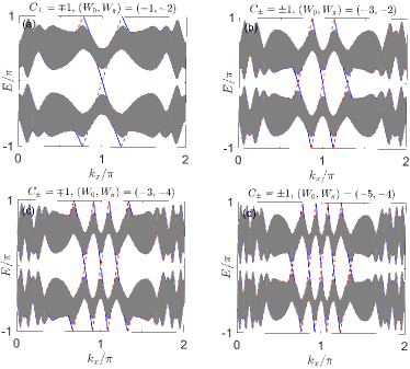
Figure B.2: (color online) The Floquet spectrum of $\hat{U}(k_{x})$ under OBC and PBC along $y$ and $x$ directions of the lattice, respectively. Gray regions represent bulk bands. Blue solid (red dashed) lines refer to edge states localized at the left (right) edge of the lattice. The lattice has $N_{y}=200$ unit cells along $y$ direction. The hopping amplitude $J_{1}$ take values as (a) $J_{1}=1.5\pi$, (b) $J_{1}=2.5\pi$, (c) $J_{1}=3.5\pi$ and (d) $J_{1}=4.5\pi$. Other system parameters are set at $(J_{2},J_{3},M)=(0.5\pi,0.2\pi,1)$. $C_{-}$ ($C_{+}$) is the Chern numbers of the lower (upper) Floquet band and $W_{0}$ ($W_{\pi}$) is the edge state winding number at quasienergy $0$ ($\pi$).

In this appendix, we present several more examples of the Floquet spectrum of $\hat{U}$ versus the hopping amplitude $J_{1}$, with the other system parameters fixed. Results under MBCX and MBCY are both studied. We see from Figs. B.1 and B.2 that the bulk and edge states configurations are similar to the cases obtained at different values of $J_{2}$ in the main text. This further demonstrate the generality of our Floquet engineering scheme in the generation of topological phases with large winding numbers and many chiral edge states.

Appendix C More examples on the Floquet spectrum

In this appendix, we present two more examples of the quasienergy spectrum of $\hat{U}(k_{y})$ at different hopping amplitudes $J_{1}=J_{2}$, with other system parameters fixed at $(J_{3},M)=(0.3\pi,1)$. Numerical results are shown in Figs. C.1 and C.2. Similar to the situation in which only one hopping amplitude ($J_{1}$ or $J_{2}$) is varied, increasing $J_{1}$ together with $J_{2}$ could also induce Chern number exchanges of the two Floquet bands and therefore the growth of the number of chiral edge states in both quasienergy gaps. Furthermore, Floquet bands with Chern numbers larger then $1$ appear in certain parameter windows. However, our numerical calculations suggest that the size of quasienergy gaps will shrink under the joint growth of $J_{1}$ and $J_{2}$, accompanied by a more complicated gap closing pattern compared with the one shown in Fig. 3(a) of the main text. These make it harder to resolve chiral edge states at larger values of $J_{1}=J_{2}$. From another perspective, the complicated topological phase pattern encountered in this situation may call for a statistical analysis of the distribution of winding numbers $(W_{0},W_{\pi})$ in a wide range of $J_{1}=J_{2}$, as considered recently in a one-dimensional system Seradjeh2017 .

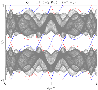
Figure C.1: (color online) The Floquet spectrum of $\hat{U}(k_{y})$ under OBC and PBC along $x$ and $y$ directions of the lattice, respectively. Gray regions represent bulk bands. Blue solid (red dashed) lines refer to edge states localized at the left (right) edge of the lattice. The lattice has $N_{x}=300$ unit cells along $x$ direction. The hopping amplitudes $J_{1}=J_{2}=1.4\pi$. Other system parameters are set at $(J_{3},M)=(0.3\pi,1)$. $C_{-}$ ($C_{+}$) is the Chern numbers of the lower (upper) Floquet band and $W_{0}$ ($W_{\pi}$) is the edge state winding number at quasienergy $0$ ($\pi$).

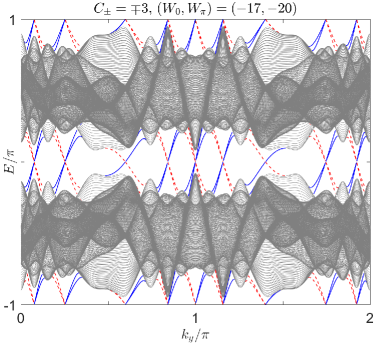
Figure C.2: (color online) The Floquet spectrum of $\hat{U}(k_{y})$ under OBC and PBC along $x$ and $y$ directions of the lattice, respectively. Gray regions represent bulk bands. Blue solid (red dashed) lines refer to edge states localized at the left (right) edge of the lattice. The lattice has $N_{y}=300$ unit cells along $x$ direction. The hopping amplitudes $J_{1}=J_{2}=2.1\pi$. Other system parameters are set at $(J_{3},M)=(0.3\pi,1)$. $C_{-}$ ($C_{+}$) is the Chern numbers of the lower (upper) Floquet band and $W_{0}$ ($W_{\pi}$) is the edge state winding number at quasienergy $0$ ($\pi$).

Appendix D Calculation of the Bott index

In this appendix, we explain a bit more on the calculation of the Bott index of our quenched lattice model. Taking a torus geometry of size $N_{x}\times N_{y}$ for the lattice (i.e., PBC along both $x$ and $y$ directions), we will have two bulk Floquet bands. We denote $P_{-}$ and $P_{+}$ as projectors to the lower and higher band in the first quasienergy Brillouin zone, respectively. In the spectrum representation, these projectors are given by:

$$P_{-}= \sum_{E\in(-\pi,0)}E|E\rangle\langle E|=V\begin{bmatrix}\mathbb{I}_{N_{1}N_{2}}&0\\ 0&0\end{bmatrix}V^{\dagger},$$ (D.1)

$$P_{+}= \sum_{E\in(0,+\pi)}E|E\rangle\langle E|=V\begin{bmatrix}0&0\\ 0&\mathbb{I}_{N_{1}N_{2}}\end{bmatrix}V^{\dagger},$$ (D.2)

where $V$ is the unitary transformation which diagonalizes the Floquet operator $\hat{U}$, i.e., $\hat{U}=Ve^{-i\sum_{E}E|E\rangle\langle E|}V^{\dagger}$.

To evaluate the Bott index, we introduce the “exponential (unitary) position operators” as Bott6 :

$$\hat{U}_{X}= \,e^{i\frac{2\pi}{N_{x}}\sum_{n_{x}=1}^{N_{x}}n_{x}|n_{x}\rangle\langle n_{x}|\otimes\mathbb{I}_{N_{y}}\otimes\sigma_{0}},$$ (D.3)

$$\hat{U}_{Y}= \,e^{i\frac{2\pi}{N_{y}}\mathbb{I}_{N_{x}}\otimes\sum_{n_{y}=1}^{N_{y}}n_{y}|n_{y}\rangle\langle n_{y}|\otimes\sigma_{0}}.$$ (D.4)

Then the projections of these operators to the lower Floquet band $U_{X-}$ and $U_{Y-}$ are given by

$$P_{-}\hat{U}_{\alpha}P_{-}=V\begin{bmatrix}U_{\alpha-}&0\\ 0&0\end{bmatrix}V^{\dagger},\qquad\alpha=X,Y.$$ (D.5)

Finally, the Bott index of the lower Floquet band $B_{-}$ reads

$$B_{-}=\frac{1}{2\pi}{\rm Im}\left\{{\rm Tr}\left[\ln\left(U_{X-}U_{Y-}U_{X-}^{\dagger}U_{Y-}^{\dagger}\right)\right]\right\}.$$ (D.6)

The numerical values of $B_{-}$ for our quenched lattice model are presented in Fig. 6 of the main text. For a clean sample, it has been shown that the Bott index of a filled band is equivalent to its Chern number Bott2 ; Bott5 . However, since the Bott index is defined on a discrete lattice in position space, it is also well-defined for a disordered system. Therefore the Bott index could be useful to describe topological phase transitions induced by disorder in both static and Floquet systems.

References

- (1) G. Jotzu, M. Messer, R. Desbuquois, M. Lebrat, T. Uehlinger, D. Greif, and T. Esslinger, Nature 515, 237 (2014); M. Aidelsburger, M. Lohse, C. Schweizer, M. Atala, J. T. Barreiro, S. Nascimbne, N. R. Cooper, I. Bloch and N. Goldman, Nat. Phys. 11, 162 (2015).
- (2) N. Fläschner, B. S. Rem, M. Tarnowski, Vogel, D.-S. Lühmann, K. Sengstock, and C. Weitenberg, Science 352, 1091 (2016).
- (3) T. Kitagawa, M. A. Broome, A. Fedrizzi, M. S. Rudner, E. Berg, I. Kassal, A. Aspuru-Guzik, E. Demler and A. G. White, Nat. Commun. 3, 882 (2012).
- (4) M. C. Rechtsman, J. M. Zeuner, Y. Plotnik, Y. Lumer, D. Podolsky, F. Dreisow, S. Nolte, M. Segev, and A. Szameit, Nature 496, 196 (2013); W. Hu, J. C. Pillay, K. Wu, M. Pasek, P. P. Shum, and Y. D. Chong, Phys. Rev. X 5, 011012 (2015).
- (5) L. J. Maczewsky, J. M. Zeuner, S. Nolte, and A. Szameit, Nat. Commun. 8, 13756 (2017); S. Mukherjee, A. Spracklen, M. Valiente, E. Andersson, P. Ohberg, N. Goldman, and R. R. Thomson, Nat. Commun. 8, 13918 (2017).
- (6) M. Xiao, G. Ma, Z. Yang, P. Sheng, Z. Q. Zhang, and C. T. Chan, Nat. Phys. 11, 240 (2015); R. Ssstrunk and S. D. Huber, Science 349, 47 (2015); R. Fleury, A. B. Khanikaev and A. Al, Nat. Commun. 7, 11744 (2016); R. Ssstrunk, P. Zimmermann, and S. D. Huber, New J. Phys. 19, 015013 (2017).
- (7) Y. Peng, C. Qin, D. Zhao, Y. Shen, X. Xu, M. Bao, H. Jia, and X. Zhu, Nat. Commun. 7, 13368 (2016).
- (8) J. Wang and J. B. Gong, Phys. Rev. A 77, 031405 (2008); J. Wang, A. S. Mouritzen, and J. Gong, J. Mod. Optics 56, 722 (2009).
- (9) T. Oka and H. Aoki, Phys. Rev. B 79, 081406 (2009).
- (10) N. H. Lindner, G. Refael, and V. Galitski, Nat. Phys. 7, 490 (2011).
- (11) J. P. Dahlhaus, J. M. Edge, J. Tworzydlo, and C. W. J. Beenakker, Phys. Rev. B 84, 115133 (2011).
- (12) T. Kitagawa, T. Oka, A. Brataas, L. Fu, and E. Demler, Phys. Rev. B 84, 235108 (2011).
- (13) D. Y. H. Ho and J. Gong, Phys. Rev. Lett. 109, 010601 (2012).
- (14) H. Wang, D. Y. H. Ho, W. Lawton, J. Wang, and J. Gong, Phys. Rev. E 88, 052920 (2013).
- (15) Q.-J. Tong, J.-H. An, J. Gong, H.-G. Luo, and C. H. Oh, Phys. Rev. B 87, 201109 (2013).
- (16) . Gmez-Len and G. Platero, Phys. Rev. Lett. 110, 200403 (2013).
- (17) J. Cayssol, B. Dra, F. Simon, and R. Moessner, Phys. Status Solidi Rapid Res. Lett. 7, 101 (2013).
- (18) M. Thakurathi, A. A. Patel, D. Sen and A. Dutta, Phys. Rev. B 88, 155133 (2013).
- (19) D. Y. H. Ho and J. Gong, Phys. Rev. B 90, 195419 (2014).
- (20) A. G. Grushin, . Gmez-Len, and T. Neupert, Phys. Rev. Lett. 112, 156801 (2014).
- (21) R. Wang, B. Wang, R. Shen, L. Sheng, and D. Y. Xing, Europhys. Lett. 105, 17004 (2014).
- (22) L. Zhou, H. Wang, D. Y. H. Ho, and J. Gong, Eur. Phys. J. B 87, 204 (2014).
- (23) P. Titum, N. H. Lindner, M. C. Rechtsman, and G. Refael, Phys. Rev. Lett. 114, 056801 (2015).
- (24) T.-S. Xiong, J. Gong, and J.-H. An, Phys. Rev. B 93, 184306 (2016).
- (25) J. Klinovaja, P. Stano, and D. Loss, Phys. Rev. Lett. 116, 176401 (2016); M. Thakurathi, D. Loss, and J. Klinovaja, Phys. Rev. B 95, 155407 (2017).
- (26) Y. Chen and C. Tian, Phys. Rev. Lett. 113, 216802 (2014); C. Tian, Y. Chen, and J. Wang, Phys. Rev. B 93, 075403 (2016).
- (27) T. Kitagawa, E. Berg, M. Rudner, and E. Demler, Phys. Rev. B 82, 235114 (2010).
- (28) L. Jiang, T. Kitagawa, J. Alicea, A. R. Akhmerov, D. Pekker, G. Refael, J. I. Cirac, E. Demler, M. D. Lukin, and P. Zoller, Phys. Rev. Lett. 106, 220402 (2011).
- (29) A. Kundu and B. Seradjeh, Phys. Rev. Lett. 111, 136402 (2013).
- (30) R. W. Bomantara, G. N. Raghava, L. Zhou, and J. Gong, Phys. Rev. E 93, 022209 (2016); R. W. Bomantara and J. Gong, Phys. Rev. B 94, 235447 (2016).
- (31) M. Lababidi, I. I. Satija, and E. Zhao, Phys. Rev. Lett. 112, 026805 (2014); Z. Zhou, I. I. Satija, and E. Zhao, Phys. Rev. B 90, 205108 (2014).
- (32) M. D. Reichl and E. J. Mueller, Phys. Rev. A 89, 063628 (2014).
- (33) . Gmez-Len, P. Delplace, and G. Platero, Phys. Rev. B 89, 205408 (2014).
- (34) M. S. Rudner, N. H. Lindner, E. Berg, and M. Levin, Phys. Rev. X 3, 031005 (2013); P. Titum, E. Berg, M. S. Rudner, G. Refael, and N. H. Lindner, Phys. Rev. X 6, 021013 (2016).
- (35) I. C. Fulga and M. Maksymenko, Phys. Rev. B 93, 075405 (2016).
- (36) H. H. Yap, L. Zhou, J. Wang, and J. Gong, Phys. Rev. B 96, 165443 (2017).
- (37) H. H. Yap, L. Zhou, C. H. Lee, J. Gong, arXiv:1711.09540 (2017).
- (38) L. Zhou, C. Chen, and J. Gong, Phys. Rev. B 94, 075443 (2016).
- (39) J. K. Asbth, Phys. Rev. B 86, 195414 (2012). J. K. Asbth, and H. Obuse, Phys. Rev. B 88, 121406 (2013).
- (40) F. Nathan and M. S. Rudner, New J. Phys. 17, 125014 (2015).
- (41) R. Roy and F. Harper, Phys. Rev. B 94, 125105 (2016); R. Roy and F. Harper, Phys. Rev. B 96, 155118 (2017).
- (42) S. Yao, Z. Yan, and Z. Wang, Phys. Rev. B 96, 195303 (2017).
- (43) X. Qi, Y. Wu, S. Zhang, Phys. Rev. B 74, 085308 (2006).
- (44) S. A. Skirlo, L. Lu, and M. Soljačić, Phys. Rev. Lett. 113, 113904 (2014); S. A. Skirlo, L. Lu, Y. Igarashi, Q. Yan, J. Joannopoulos, and M. Soljačić, Phys. Rev. Lett. 115, 253901 (2015).
- (45) G. Miert, C. M. Smith, and V. Juričić, Phys. Rev. B 90, 081406(R) (2014).
- (46) J. Röntynen and T. Ojanen, Phys. Rev. Lett. 114, 236803 (2015).
- (47) T. Chen, Z. Xiao, D. Chiou, and G. Guo, Phy. Rev. B 84, 165453 (2011).
- (48) H. Jiang, Z. H. Qiao, W. Liu, and Q. Niu, Phys. Rev. B 85, 045445 (2012).
- (49) J. Wang, B. Lian, H. Zhang, Y. Xu, and S. Zhang, Phys. Rev. Lett. 111, 136801 (2013).
- (50) C. Fang, M. J. Gilbert, and B. A. Bernevig, Phys. Rev. Lett. 112, 046801 (2014).
- (51) P. M. Perez-Piskunow, L. E. F. Foa Torres, and G. Usaj, Phys. Rev. A 91, 043625 (2015).
- (52) Y. V. Fyodorov and H. J. Sommers, JETP Lett. 72, 422 (2000).
- (53) A. Ossipov, T. Kottos, and T. Geisel, Phys. Rev. E 65, 055209 (2002).
- (54) J. P. Dahlhaus, J. M. Edge, J. Tworzydlo, and C. W. J. Beenakker, Phys. Rev. B 84, 115133 (2011).
- (55) A. Tajic, Ph.D. thesis, Leiden University, 2005.
- (56) I. C. Fulga and M. Maksymenko, Phys. Rev. B 93, 075405 (2016).
- (57) R. Ducatez and F. Huveneers, Annales Henri Poincaré 18, 2415 (2017).
- (58) T. A. Loring and M. B. Hastings, EPL 92, 67004 (2011).
- (59) L. D’Alessio and M. Rigol, Nat. Commun. 6, 8336 (2015).
- (60) P. Titum, N. H. Lindner, and G. Refael, Phys. Rev. B 96, 054207 (2017).
- (61) D. Toniolo, arXiv:1708.05912 (2017).
- (62) O. Shtanko, R. Movassagh, arXiv:1803.08519 (2018).
- (63) E. Prodan, A Computational Non-Commutative Geometry Program for Disordered Topological Insulators (Springer, Switzerland, 2017).
- (64) S. Shen, Topological Insulators, Second Edition (Springer, Singapore, 2017).
- (65) M. Rodriguez-Vega and B. Seradjeh, arXiv:1706.05303 (2017).