Signatures of chaos and thermalization
in the dynamics of many-body quantum systems

Abstract

We extend the results of two of our papers [Phys. Rev. A 94, 041603R (2016) and Phys. Rev. B 97, 060303R (2018)] that touch upon the intimately connected topics of quantum chaos and thermalization. In the first, we argued that when the initial state of isolated lattice many-body quantum systems is chaotic, the power-law decay of the survival probability is caused by the bounds in the spectrum, and thus anticipates thermalization. In the current work, we provide stronger numerical support for the onset of these algebraic behaviors. In the second paper, we demonstrated that the correlation hole, which is a direct signature of quantum chaos revealed by the evolution of the survival probability at times beyond the power-law decay, appears also for other observables. In the present work, we investigate the correlation hole in the chaotic regime and in the vicinity of a many-body localized phase for the spin density imbalance, which is an observable studied experimentally.

I Introduction

The description of the dynamics of many-body quantum systems perturbed far from equilibrium involves several obstacles. Analytical studies are mostly restricted to integrable models, while the systems are often nonintegrable. Approximations, such as perturbation theory, can capture the behavior of limited time intervals, but different behaviors emerge at different time scales. Furthermore, the dynamics depends on the model, initial state, and observable investigated, which hinders attempts of generalizations.

A useful approach, advocated in Ref. Torres-Herrera et al. (2018), is to study the evolution under full random matrices (FRM), since they allow for the derivation of analytical expressions for any observable at any time. The results can then be used to guide the analysis of realistic chaotic models. FRM from Gaussian orthogonal ensembles (GOEs) are symmetric matrices filled with real random numbers. They were employed by Wigner in the 50’s to describe statistically the spectra of heavy nuclei Wigner (1951, 1958). They are unphysical, because they imply the simultaneous interactions of all particles, but they provide relevant information about the level statistics of real systems Mehta (1991); Guhr et al. (1998); Stöckmann (2006). We have transferred this approach to the study of dynamics. Combining the fact that the eigenstates of FRM are random vectors and that several studies about the correlations among the eigenvalues already exist, one can study the dynamics analytically. Based on the results obtained with FRM, we can then anticipate and justify the behaviors of realistic many-body quantum systems that show GOE level statistics.

The eigenvalues of FRM are correlated; they are prohibited from crossing. Level repulsion is a main signature of quantum chaos. One-body quantum systems that show level repulsion and have a rigid spectrum are known to be chaotic in the classical limit Stöckmann (2006). This has been shown numerically and through semiclassical treatments. As often done, we extend this notion to many-body quantum systems and refer to them as chaotic if they show level repulsion. We note, however, that the relationship between level statistics and classical chaos for many-body quantum systems has not yet been demonstrated.

In several of our studies of the nonequilibrium dynamics of many-body quantum systems Zangara et al. (2013); Torres-Herrera and Santos (2014a, b, c); Torres-Herrera et al. (2015, 2014); Torres-Herrera and Santos (2014d); Torres-Herrera and Santos (2015); Torres-Herrera et al. (2016a, b); Távora et al. (2016, 2017); Torres-Herrera and Santos (2017a, b); del Campo et al. ; Torres-Herrera et al. (2018); Santos and Torres-Herrera (2017), we focused on a simple observable, namely the survival probability, which is the probability of finding the system still in its initial state later in time. In hands of a good understanding of the evolution of this quantity, we can then proceed with the analysis of particular observables Torres-Herrera et al. (2014, 2018).

The survival probability for GOE-FRM and, equivalently, for chaotic many-body quantum systems shows the following generic behaviors Torres-Herrera et al. (2018). At short times, the decay is quadratic and universal. Next, the evolution depends on the shape and bounds of the energy distribution of the initial state Torres-Herrera and Santos (2014a, b); Torres-Herrera et al. (2014); Torres-Herrera and Santos (2014d). In systems perturbed far from equilibrium, where this energy distribution is broad and dense, the decay can initially be very fast, but it subsequently slows down and becomes power law, due to the presence of the unavoidable bounds in the spectrum, which causes the partial reconstruction of the initial state Távora et al. (2016, 2017); Khalfin (1958); Ersak (1969); Fleming (1973); Knight (1977); Fonda et al. (1978); Sluis and Gislason (1991); Urbanowski (2009); del Campo (2011, 2016); Muga et al. (2009). Following the algebraic decay, one finds the correlation hole, which is a dip below the saturation of the dynamics Torres-Herrera and Santos (2017b); del Campo et al. ; Torres-Herrera et al. (2018); Santos and Torres-Herrera (2017) caused by short- and long-correlations between the eigenvalues of chaotic models Leviandier et al. (1986); Guhr and Weidenmüller (1990); Wilkie and Brumer (1991); Alhassid and Levine (1992); Gorin and Seligman (2002). The saturation to a finite value larger than zero is the last step of the evolution and happens because the systems investigated are finite Zangara et al. (2013).

One needs highly delocalized initial states, large system sizes, and preferably chaotic models to observe the power-law decay of the survival probability induced by the energy bounds. This is because the dynamics needs to detect the energy bounds before detecting the discreteness of the spectrum. Initial states that are so delocalized that most overlaps with the energy eigenbasis are close to random numbers satisfy this criterion. These are chaotic states and they guarantee the onset of thermalization Rigol and Srednicki (2012); Torres-Herrera and Santos (2013); Borgonovi et al. (2016).

The power-law behavior of the survival probability caused by the bounds of the spectrum is evident in FRM of relatively small dimensions, but for realistic models, our numerical results in Távora et al. (2016, 2017) were not as convincing. We remedy this situation here by showing results for large system sizes averaged over delocalized initial states and disorder realizations. We consider a one-dimensional (1D) spin-1/2 model with onsite disorder. Averages over initial states and disorder realizations smoothen the curves and reveal the expected algebraic decay.

In Ref. Torres-Herrera et al. (2018), using GOE-FRM, we obtained an expression for the entire evolution of the survival probability and also for the spin density imbalance, which is an observable measured experimentally Schreiber et al. (2015); Bordia et al. (2017). The results revealed the presence of the correlation hole for both quantities, indicating that the hole is not exclusive to the survival probability. The correlation hole is an unambiguous signature of quantum chaos and since chaos guarantees that isolated many-body quantum systems reach thermal equilibrium Borgonovi et al. (2016); D’Alessio et al. (2016), the presence of the correlation hole also assures thermalization. In the present work, we consider the disordered 1D spin model mentioned above and analyze the correlation hole for the spin density imbalance. We show how the depth of the hole depends on the strength of the disorder and how it vanishes with the approach to a localized phase.

II Disordered spin-1/2 model

The Hamiltonian of the isolated disordered 1D spin-1/2 model that we study is

$$H=H_{0}+V,$$ (1)

where

$$H_{0}=\sum_{k=1}^{L}h_{k}S_{k}^{z}\hskip 11.38092pt{\rm and}\hskip 11.38092ptV=J\sum_{k=1}^{L}\left(S_{k}^{x}S_{k+1}^{x}+S_{k}^{y}S_{k+1}^{y}+S_{k}^{z}S_{k+1}^{z}\right).$$ (2)

The chain has $L$ sites and periodic boundary conditions. $S_{k}^{x,y,z}$ are the spin operators on site $k$, $J$ is the coupling parameter, which we set to 1, and the Zeeman splittings $h_{k}$ are random numbers from a uniform distribution with support $[-h,h]$, $h$ being the disorder strength. Hamiltonian $H$ conserves the total spin in the $z$-direction, ${\cal S}^{z}=\sum_{k}S_{k}^{z}$. We focus on the largest subspace, ${\cal S}^{z}=0$, which has dimension ${\cal D}=L!/(L/2)!^{2}$. We list below important features of the disordered spin model, which will be used in the paper.

(i) It represents a many-body quantum system with two-body interactions only, which implies that the density of states is Gaussian Brody et al. (1981); Kota (2001). This is in contrast with the density of states of FRM, which has a semicircular shape Mehta (1991); Guhr et al. (1998); Stöckmann (2006).

(ii) When the disorder strength $h$ is of the order of the coupling parameter, $h\sim 1$, the eigenvalues of $H$ show strong level repulsion Santos (2004); Santos et al. (2004); Dukesz et al. (2009). The distribution $P(s)$ of the spacings $s$ between neighboring levels follows the one for GOE-FRM Guhr et al. (1998), $P_{GOE}(s)=\frac{\pi}{2}s\exp\left(-\frac{\pi}{4}s^{2}\right)$. For the system sizes available to exact diagonalization, the best agreement with $P_{GOE}(s)$ happens for $h\sim 0.5$ Torres-Herrera and Santos (2017a).

(iii) As $h$ increases above the coupling parameter, the system moves away from the chaotic region and approaches a localized phase in space Santos et al. (2004); Basko et al. (2006); Oganesyan and Huse (2007); Dukesz et al. (2009); Torres-Herrera and Santos (2015); Torres-Herrera and Santos (2017a), despite the presence of interactions. In this limit, the eigenvalues are no longer correlated and $P(s)$ no longer agrees with $P_{GOE}(s)$.

III Quench Dynamics and Observables

We prepare the system in the initial state $|\Psi(0)\rangle\equiv|n_{0}\rangle$, where $|n_{0}\rangle$ is one of the eigenstates $|n\rangle$ of the initial Hamiltonian $H_{0}$ [Eq. (2)]. These states are site-basis vectors, where on each site there is either a spin pointing up in the $z$-direction or pointing down. The system is then perturbed far from equilibrium and let to evolve under the new total Hamiltonian $H$ [Eq. (1)]. The evolved state is given by

$$|\Psi(t)\rangle=e^{-iHt}|\Psi(0)\rangle=\sum_{\alpha}C_{n_{0}}^{\alpha}e^{-iE_{\alpha}t}|\alpha\rangle,$$

where $C^{\alpha}_{n_{0}}=\langle\alpha|\Psi(0)\rangle$ and $H|\alpha\rangle=E_{\alpha}|\alpha\rangle$.

The two observables that we study are (i) the survival probability and (ii) the spin density imbalance.

(i) The survival probability corresponds to

$$W_{n_{0}}(t)=\left|\langle\Psi(0)|\Psi(t)\rangle\right|^{2}=\left|\sum_{\alpha}\left|C_{n_{0}}^{\alpha}\right|^{2}e^{-iE_{\alpha}t}\right|^{2}.$$ (3)

For very short times, by expanding the exponential, one sees that

$$W_{n_{0}}(t)\approx 1-\sigma_{n_{0}}^{2}t^{2},$$ (4)

where

$$\sigma_{n_{0}}^{2}=\sum_{\alpha}|C^{\alpha}_{n_{0}}|^{2}(E_{\alpha}-E_{n_{0}})^{2}$$ (5)

is the energy variance of the initial state and

$$E_{n_{0}}=\langle\Psi(0)|H|\Psi(0)\rangle=\sum_{\alpha}|C^{\alpha}_{n_{0}}|^{2}E_{\alpha}$$ (6)

is its energy. The quadratic decay in Eq. (4) is universal and holds when $t\ll\sigma_{n_{0}}^{-1}$.

Equation (3) can also be written as

$$W_{n_{0}}(t)=\left|\int_{E_{low}}^{E_{up}}dE\,e^{-iEt}\rho_{n_{0}}(E)\right|^{2},$$ (7)

where $E_{low}$ and $E_{up}$ are the lower and upper bounds of the energy spectrum and

$$\rho_{n_{0}}(E)\equiv\sum_{\alpha}|C^{\alpha}_{n_{0}}|^{2}\delta(E-E_{\alpha})$$ (8)

is the local density of states (LDOS), that is the energy distribution weighted by the components $|C^{\alpha}_{n_{0}}|^{2}$ of the initial state. Therefore, $W_{n_{0}}(t)$ is the absolute square of the Fourier transform of the LDOS and $\sigma_{n_{0}}$ is the width of the LDOS.

(ii) The spin density imbalance Luitz et al. (2016); Lee et al. (2017),

$$I(t)=\frac{4}{L}\sum_{k=1}^{L}S^{z}_{k}(0)\langle\Psi(0)|S^{z}_{k}(t)|\Psi(0)\rangle,$$ (9)

is the sum of the correlation in time of the magnetization in the $z$-direction of each site $k$. It is equivalent to the density imbalance measured in experiments with cold atoms Schreiber et al. (2015); Bordia et al. (2017).

IV Power-law decay

Starting the dynamics with an eigenstate of $H_{0}$ [Eq. (2)] and letting it evolve according to $H$ [Eq. (1)] implies that a very strong perturbation is applied to the system. It is equivalent to suddenly changing the coupling parameter $J$ from 0 to 1. In the limit of very strong perturbation, the LDOS has a shape similar to the density of states Torres-Herrera et al. (2014), which in our case, as mentioned in Sec. II, is Gaussian. If the energy of the initial state is close to the middle of the spectrum, $E_{n_{0}}\sim 0$, the Gaussian LDOS is nearly symmetric, while the proximity of $E_{n_{0}}$ to the borders of the spectrum gives rise to skewed distributions Torres-Herrera and Santos (2014d).

The Fourier transform of a Gaussian LDOS leads to the Gaussian decay of the survival probability, $W_{n_{0}}(t)=\exp(-\sigma_{n_{0}}^{2}t^{2})$, as confirmed by our previous works Torres-Herrera and Santos (2014a, b, c); Torres-Herrera et al. (2014); Torres-Herrera and Santos (2014d). However, due to the energy bounds $E_{low}$ and $E_{up}$, the decay is not entirely Gaussian, but given by Távora et al. (2016, 2017)

$$W_{n_{0}}(t) =\left|\frac{1}{{\cal N}\sqrt{2\pi\sigma_{n_{0}}^{2}}}\int_{E_{low}}^{E_{up}}dE\,e^{-iEt}e^{-(E-E_{n_{0}})^{2}/2\sigma_{n_{0}}^{2}}\right|^{2}$$

$$=\frac{e^{-\sigma_{n_{0}}^{2}t^{2}}}{4{\cal N}^{2}}\left|\left[{\rm erf}\left(\frac{E_{n_{0}}-E_{low}+i\sigma_{n_{0}}^{2}t}{\sqrt{2\sigma_{n_{0}}^{2}}}\right)-{\rm erf}\left(\frac{E_{n_{0}}-E_{up}+i\sigma_{n_{0}}^{2}t}{\sqrt{2\sigma_{n_{0}}^{2}}}\right)\right]\right|^{2},$$ (10)

where

$${\cal N}=\frac{1}{2}\left[{\rm erf}\left(\frac{E_{n_{0}}-E_{low}}{\sqrt{2\sigma_{n_{0}}^{2}}}\right)-{\rm erf}\left(\frac{E_{n_{0}}-E_{up}}{\sqrt{2\sigma_{n_{0}}^{2}}}\right)\right]$$ (11)

is a normalization constant and erf is the error function. In the limit $t\gg\sigma_{n_{0}}^{-1}$, after averaging out the oscillations, we get

$$W_{n_{0}}(t\gg\sigma_{n_{0}}^{-1})\simeq\frac{1}{2\pi{\cal N}^{2}\sigma_{n_{0}}^{2}t^{2}}\left[e^{-(E_{up}-E_{n_{0}})^{2}/\sigma_{n_{0}}^{2}}+e^{-(E_{low}-E_{n_{0}})^{2}/\sigma_{n_{0}}^{2}}\right],$$ (12)

which indicates that a power-law decay $\propto t^{-2}$ should follow the Gaussian behavior.

In general, the power-law exponent $\gamma$ of $W_{n_{0}}\propto t^{-\gamma}$ depends on how the LDOS approaches the energy bounds. Asymptotic studies Erdélyi (1956); Urbanowski (2009) have shown that

$$\gamma=2(\xi+1)\hskip 8.5359pt{\rm for}\hskip 8.5359pt\rho_{n_{0}}(E)=(E-E_{low})^{\xi}\eta(E),$$ (13)

where $\lim_{E\rightarrow E_{low}}\eta(E)>0$ (or equivalent for $E_{up}$ if $E_{n_{0}}$ is closer to the upper bound). In the case of Gaussian or Lorentzian tails, where $\xi\sim 0$, we have that $\gamma=2$ (see Appendix of Távora et al. (2017)).

The results in Eq. (10) and Eq. (13) actually presuppose a continuous spectrum, which is not at all our case. The envelope of our LDOS has a Gaussian shape, but the distribution is obtained from a discrete spectrum. Yet, for enough large ${\cal D}$ and for initial states that are highly delocalized, it takes a long time for the dynamics to resolve the discreteness of the spectrum. Until then, the evolution is equivalent to what we would find in the continuum.

Highly delocalized initial states appear in the limit of very strong perturbations and for energies $E_{n_{0}}$ close to the middle of the spectrum. They show up when $H$ (or at least $H_{0}$) is chaotic. Such chaotic initial states guarantee the onset of thermalization Rigol and Srednicki (2012); Torres-Herrera and Santos (2013); Borgonovi et al. (2016). This led us to claim in Refs. Távora et al. (2016, 2017) that in isolated lattice many-body quantum systems with two-body interactions, the emergence of power-law decays given by $W_{n_{0}}(t)\propto t^{-2}$ indicate that the initial state will eventually reach thermal equilibrium.

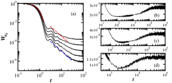
Figure 1: Survival probability for the disordered spin-1/2 model. In (a), the system is in the chaotic regime, $h=0.5$, and the curves from top to bottom are for $L=16,18,20,22,24$. For $L$ from $16$ to $22$ the average is over $9$ different initial states and over $120$ different disorder realizations. For $L=24$ the average is over $1$ initial state and over $120$ disorder realizations. The top dashed line represents $W_{n_{0}}(t)\propto t^{-2}$. The bottom dashed line is a fitting for the curve with $L=24$ for $t\in[3,30]$, which gives $W_{n_{0}}(t)\simeq 0.001t^{-2}$. The circles are for $W_{n_{0}}(t)=\exp(-\sigma_{n_{0}}^{2}t^{2})$ for $L=16$. On the right panels, we show $W_{n_{0}}(t)$ for $L=16$ at long times, where the correlation hole emerges. The disorder strengths are $h=0.5$ (b), $h=1$ (c), and $h=1.5$ (c); averages over $1287$ initial states and $77$ disorder realizations. All initial states have $E_{n_{0}}\sim 0$.

In Fig. 1 (a), we show $W_{n_{0}}(t)$ for $H$ in the chaotic limit ($h=0.5$). System sizes from $L=16$ to $L=24$ are considered. For $L>16$, our computers do not have memory to performing exact diagonalization. To handle such large $L$’s, we use the software package EXPOKIT Sidje (1998); Exp . Since exact diagonalization of $H$ is not available, to guarantee the selection of initial states with $E_{n_{0}}\sim 0$ and avoid the borders of the spectrum, we choose initial states with energy $\langle\Psi(0)|H_{0}|\Psi(0)\rangle\sim 0$. The curves are smoothened by averages over disorder realizations and different initial states.

In Fig. 1 (a), the initial decay of $W_{n_{0}}(t)$ is indeed Gaussian, as anticipated. It is not only the universal quadratic behavior for $t\ll\sigma_{n_{0}}^{-1}$ presented in Eq. (4), but a true Gaussian decay that holds for times up to $t\sim\sigma_{n_{0}}^{-1}$.

The algebraic decay of $W_{n_{0}}(t)$ dominates after a time $t_{P}$ obtained from the crossing point between the fast Gaussian decay and the slower power-law behavior Távora et al. (2017), $e^{-\sigma_{n_{0}}^{2}t_{P}^{2}}\sim W_{n_{0}}(t_{P}\gg\sigma_{0}^{-1})$. As seen in Fig. 1 (a), after the Gaussian behavior, $W_{n_{0}}(t)$ decays as $t^{-2}$. Notice that the interval of the power-law decay holds for longer as $L$ increases. This picture is analogous to what one finds for GOE-FRM and implies that equilibration should take longer to happen as the system size increases.

To compare the results above with those for the GOE, we assume that $H_{0}$ is the diagonal of the FRM and $H$ is the total random matrix. In this case the shape of the envelope of the LDOS is semicircle Torres-Herrera and Santos (2014a); Santos and Torres-Herrera , such as the density of states of FRM. The Fourier transform of the semicircle leads to $W_{n_{0}}(t)={\cal{J}}_{1}^{2}(2\sigma_{n_{0}}t)/\sigma_{n_{0}}^{2}t^{2}$, where ${\cal J}_{1}$ is the Bessel function of the first kind. The Bessel function gives rise to oscillations that decay as $t^{-3}$ (see e.g. Fig. 1 (a) of Ref. Torres-Herrera et al. (2018)). The power-law exponent $\gamma=3$ can be justified with Eq. (13), using the fact that $\rho_{n_{0}}(E)$ for FRM approaches the energy bounds as $E^{1/2}$, that is $\xi=1/2$. Similarly to the disordered spin model, the time interval of the power-law decay of the oscillations under FRM increases with ${\cal D}$, while for very small dimensions, the power-law decay is not observed (see e.g. Fig. 1 (b) of Ref. del Campo et al. ). The results for FRM serve as a reference for the analysis of the dynamics of the realistic chaotic spin model. Even if the numerical results for real systems are limited by the accessible system sizes, the claims of the $t^{-2}$ behavior are supported by the theory and by the analogous results obtained with FRM.

V Correlation hole for the survival probability

Realistic systems are finite, so $W_{n_{0}}(t)$ does not decay to zero. In the absence of too many degeneracies, it saturates to the infinite time average

$$\overline{W}_{n_{0}}=\sum_{\alpha}\left|C_{n_{0}}^{\alpha}\right|^{4}.$$ (14)

$\overline{W}_{n_{0}}$ measures the level of delocalization of the initial state in the energy eigenbasis. In chaotic initial states, $\overline{W}_{n_{0}}\propto{\cal D}^{-1}$.

Between the power-law decay and the saturation of the dynamics, one more feature emerges in systems with level repulsion. It corresponds to a dip below the saturation value known as correlation hole. This dip appears only in systems with correlated eigenvalues, being nonexistent in integrable models. It takes a long time to show up, since the dynamics needs to resolve the discreteness of the spectrum.

In Ref. Torres-Herrera et al. (2018), we obtained an expression for the entire evolution of the survival probability evolving under GOE-FRM, which includes the correlation hole. Details can be found in Santos and Torres-Herrera (2017) and Alhassid and Levine (1992); Mehta (1991). The basic idea is to write the survival probability in terms of an integral as

$$W_{n_{0}}(t)=\int G(E)e^{-iEt}dE+\overline{W}_{n_{0}},$$ (15)

where

$$G(E)=\sum_{\alpha_{1}\neq\alpha_{2}}|C^{\alpha_{1}}_{n_{0}}|^{2}|C^{\alpha_{2}}_{n_{0}}|^{2}\delta(E-E_{\alpha_{1}}+E_{\alpha_{2}})$$ (16)

and $\overline{W}_{n_{0}}$ is given by Eq. (14). The eigenvalues and eigenstates of FRM are statistically independent. In fact, the eigenstates of FRM are random vectors. This is why one can easily get analytical results using FRM. The spectral autocorrelation function $G(E)$ can then be separated into $\langle\sum_{\alpha_{1}\neq\alpha_{2}}|C^{\alpha_{1}}_{n_{0}}|^{2}|C^{\alpha_{2}}_{n_{0}}|^{2}\rangle_{\text{FRM}}=1-\langle\overline{W}_{n_{0}}\rangle_{\rm{FRM}}$ and $\langle\delta(E-E_{\alpha_{1}}+E_{\alpha_{2}})\rangle_{\text{FRM}}$, where $\langle.\rangle_{\rm{FRM}}$ represents the average over ensembles of random matrices.

The term $\langle\delta(E-E_{\alpha_{1}}+E_{\alpha_{2}})\rangle_{\text{FRM}}$ splits into two. One is the Fourier transform of the envelope of the density of states, which leads to a term involving a Bessel function, as described above. The other term detects the discreteness of the spectrum and the correlations between the eigenvalues. It leads to the two-level form factor

$$b_{2}(\overline{t})=[1-2\overline{t}+\overline{t}\ln(1+2\overline{t})]\Theta(1-\overline{t})+\{-1+\overline{t}\ln[(2\overline{t}+1)/(2\overline{t}-1)]\}\Theta(\overline{t}-1),$$ (17)

where $\Theta$ is the Heaviside step function. Thus, the entire expression for the survival probability is Torres-Herrera et al. (2018)

$$\langle W_{n_{0}}(t)\rangle_{\rm{FRM}}=\frac{1-\langle\overline{W}_{n_{0}}\rangle_{\rm{FRM}}}{{\cal D}-1}\left[4{\cal D}\frac{{\cal J}_{1}^{2}({\cal E}t)}{({\cal E}t)^{2}}-b_{2}\left(\frac{{\cal E}t}{4{\cal D}}\right)\right]+\langle\overline{W}_{n_{0}}\rangle_{\rm{FRM}},$$ (18)

where $\pm{\cal E}$ are the energy bounds of the spectrum. The $b_{2}$ function dominates the dynamics at long times, during the time interval where the correlation hole appears. This function is directly related with the level number variance Mehta (1991); Guhr et al. (1998); Stöckmann (2006), which detects long-range correlations between the eigenvalues and is another useful quantity to diagnose quantum chaos. This explains why the hole emerges only in systems with correlated eigenvalues.

As shown in Torres-Herrera et al. (2018), the $b_{2}$ function in Eq. (17) describes not only the correlation hole for FRM, but also for the chaotic disordered model with $h=0.5$. At such long times, the dynamics depends only on the level of correlations between the eigenvalues and no longer on details about the model and initial state.

On the right panels of Fig. 1, we show the correlation hole for different values of the disorder strength: $h=0.5$ (b), $h=1$ (c), and $h=1.5$ (d). The hole fades away as the disorder increases and the system leaves the chaotic region. The hole also gets postponed to later times. The dependence of the time for the correlation hole on the disorder strength and system size, in connection with the notion of Thouless energy, is the subject of a forthcoming paper.

VI Correlation hole for the spin density imbalance

In Ref. Torres-Herrera et al. (2018), we also obtained an expression for the entire evolution of the spin density imbalance evolving under FRM, which made evident that the correlation hole is not exclusive to the survival probability. The basic steps for the derivation go as follows. For a generic observable $O$, its dynamics is given by

$$O(t)=\int K(E)e^{-iEt}dE+\overline{O},$$ (19)

where

$$K(E)=\sum_{\alpha_{1}\neq\alpha_{2}}C^{\alpha_{1}}_{n_{0}}C^{\alpha_{2}}_{n_{0}}O_{\alpha_{1}\alpha_{2}}\delta(E-E_{\alpha_{1}}+E_{\alpha_{2}}),$$ (20)

$O_{\alpha_{1}\alpha_{2}}=\langle\alpha_{1}|O|\alpha_{2}\rangle$, and

$$\overline{O}=\sum_{\alpha}|C^{\alpha}_{n_{0}}|^{2}O_{\alpha\alpha}$$ (21)

is the infinite time average. In the FRM model, since the eigenvalues and eigenstates are statistically independent, $K(E)$ splits into

$$\left\langle\sum_{\alpha_{1}\neq\alpha_{2}}C^{\alpha_{1}}_{n_{0}}C^{\alpha_{2}}_{n_{0}}O_{\alpha_{1}\alpha_{2}}\right\rangle_{\text{FRM}} =\left\langle\sum_{\alpha_{1},\alpha_{2}}C^{\alpha_{1}}_{n_{0}}C^{\alpha_{2}}_{n_{0}}O_{\alpha_{1}\alpha_{2}}\right\rangle_{\text{FRM}}-\left\langle\sum_{\alpha}|C^{\alpha}_{n_{0}}|^{2}O_{\alpha\alpha}\right\rangle_{\text{FRM}}$$

$$=O(0)-\langle\overline{O}\rangle_{\text{FRM}}$$

and $\langle\delta(E-E_{\alpha_{1}}+E_{\alpha_{2}})\rangle_{\text{FRM}}$. According to the derivation of Eq. (18) we find that

$$\langle I(t)\rangle_{\text{FRM}} =\left[I(0)-\langle\overline{I}\rangle_{\text{FRM}}\right]\left[\frac{\langle W_{n_{0}}(t)\rangle_{\rm{FRM}}-\langle\overline{W}_{n_{0}}\rangle_{\rm{FRM}}}{1-\langle\overline{W}_{n_{0}}\rangle_{\rm{FRM}}}\right]+\langle\overline{I}\rangle_{\text{FRM}}$$ (22)

$$=\frac{I(0)-\langle\overline{I}\rangle_{\text{FRM}}}{{\cal D}-1}\left[4{\cal D}\cfrac{{\cal J}_{1}^{2}(\varepsilon t)}{(\varepsilon t)^{2}}-b_{2}\left(\cfrac{\varepsilon t}{4{\cal D}}\right)\right]+\langle\overline{I}\rangle_{\text{FRM}}.$$ (23)

From Eq. (22), it is clear that the evolution of the spin density imbalance is controlled by $\langle W_{n_{0}}(t)\rangle_{\rm{FRM}}$. The $t^{-3}$ decay of the oscillations and the onset of the correlation hole, seen for the survival probability, are observed also for $\langle I(t)\rangle_{\text{FRM}}$ (see the bottom curve of the Fig. 2 of Ref. Torres-Herrera et al. (2018)).

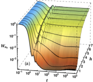
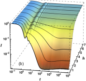
Figure 2: Survival probability and spin density imbalance for the disordered spin-1/2 model for different disorder strengths. From bottom to top: $h=0.5,1.0,1.5,2.0,2.5,3.5,4.5,5.5,6.25,7.0$. Average over $1\,287$ initial states with energy close to zero and $77$ disorder realizations.

A similar relationship between $I(t)$ and $W_{n_{0}}(t)$ is expected also for the disordered spin-1/2 model. As discussed in Torres-Herrera et al. (2014), for an observable $O$ that commutes with $H_{0}$, we have

$$O(t)=O(0)W_{n_{0}}(t)+\sum_{n\neq n_{0}}O_{nn}\left|\sum_{\alpha}C_{n}^{\alpha}C_{n_{0}}^{\alpha}e^{-iE_{\alpha}t}\right|^{2}.$$ (24)

The first term controls the short-time dynamics Torres-Herrera et al. (2014), but at long times, the dynamics depends also on the second term. An expression for $W_{n_{0}}(t)$ for realistic chaotic systems is available in Torres-Herrera et al. (2018), but further studies are required for obtaining good approximations for the second term.

The similarity between the behavior of $W_{n_{0}}(t)$ and $I(t)$ is confirmed in Fig. 2. For both quantities the initial decay is Gaussian, the oscillations appear at approximately the same time intervals, the correlation hole for $h=0.5$ is well described Torres-Herrera et al. (2018) by the $b_{2}$ function from Eq. (17), and the hole fades away as the disorder strength increases.

VII Dependence on disorder strength

In the real system, the results for the power-law decay and the correlation hole for both the survival probability and the spin density imbalance depend on the value of the disorder strength.

VII.1 Power-law decay versus disorder strength

In $W_{n_{0}}(t)$, the source of the power-law decay of the oscillations depends on the disorder strength. When the system is strongly chaotic and the LDOS is ergodically filled, such as when $h\sim 0.5$, the power-law decay is caused by the bounds in the spectrum. As the disorder strength increases above $0.5$ and the system approaches spatial localization, the LDOS ceases to be ergodically filled. As shown in Ref. Torres-Herrera and Santos (2015), for $h>1$, the power-law decay of $W_{n_{0}}(t)$ is no longer caused by the energy bounds, but by correlations between the eigenstates, which become fractal. In this scenario, the power-law exponents become smaller than 1. The transition region between the two different power-law behaviors is suggested by the bifurcation seen in Fig. 2 (a): after the Gaussian decay, the first dip for $h>1$ bifurcates into oscillations for $h<1$. These oscillations must be caused by energy bounds. In contrast, the oscillations seen for $h>1$ must be related with the onset of fractal eigenstates. By comparing Fig. 2 (a) and Fig. 2 (b), one sees that the same features hold also for the spin density imbalance.

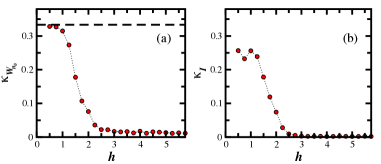
Figure 3: Depth $\kappa$ of the correlation hole for the survival probability (a) and spin density imbalance (b) versus the disorder strength for $h\geq 0.5$. The dashed line indicates the maximum $\left(\kappa_{W_{n_{0}}}\right)_{\text{FRM}}=1/3$ obtained for the survival probability evolving under FRM. $L=16$, averages over $1\,287$ initial states and $77$ disorder realizations

VII.2 Correlation hole versus disorder strength

The lowest point of the correlation hole happens at similar times for the survival probability and spin density imbalance. Equivalently to what we did for the survival probability in Ref. Torres-Herrera and Santos (2017b), we use here the depth of the correlation hole for the density imbalance to indicate the transition from the chaotic region to the many-body localized phase. We compute

$$\kappa=\frac{\langle\overline{O}\rangle-\langle O_{min}\rangle}{\langle\overline{O}\rangle},$$ (25)

where $\langle O_{min}\rangle$ is the minimum value of $\langle O(t)\rangle$. In Fig. 3 (a), $O=W_{n_{0}}$ and in Fig. 3 (b), $O=I$.

The maximum values of $\kappa_{W_{n_{0}}}$ and $\kappa_{I}$ happen for FRM. To obtain the infinite time average for GOE-FRM, we use the fact that the coefficients $C_{n_{0}}^{\alpha}$ are random numbers from a Gaussian distribution and satisfy the normalization condition $\sum_{\alpha}|C_{n_{0}}^{\alpha}|^{2}=1$. This implies that

$$\sum_{\alpha}|C_{n_{0}}^{\alpha}|^{4}=\frac{3}{{\cal{D}}+2}\quad\Rightarrow\quad\langle\overline{W}_{n_{0}}\rangle_{\rm{FRM}}=\frac{3}{{\cal D}+2}$$ (26)

and

$$\sum_{\alpha}|C_{n_{0}}^{\alpha}|^{2}|C_{n}^{\alpha}|^{2}=\frac{1}{{\cal{D}}+2}\quad\Rightarrow\quad\langle\overline{I}\rangle_{\rm{FRM}}=\frac{2}{{\cal D}+2}\,.$$ (27)

Using Eq. (21), the result above is explained as follows:

$$\langle\overline{I}\rangle_{\rm{FRM}}=\sum_{\alpha}|C_{n_{0}}^{\alpha}|^{2}I_{\alpha\alpha}=\sum_{n}I_{nn}\left(\sum_{\alpha}|C_{n_{0}}^{\alpha}|^{2}|C_{n}^{\alpha}|^{2}\right),$$ (28)

where

$$I_{nn}=\frac{4}{L}\sum_{k}\langle n_{0}|S_{k}^{z}|n_{0}\rangle\langle n|S_{k}^{z}|n\rangle.$$

Among all $I_{nn}$, ${\cal D}/2$ of them equal $+1$ and ${\cal D}/2$ of them equal $-1$. Thus, they all cancel in the sum in Eq. (28), except for two, because the value of $\sum_{\alpha}|C_{n_{0}}^{\alpha}|^{2}|C_{n}^{\alpha}|^{2}$ for $n=n_{0}$ is not the same as for $n\neq n_{0}$. Since $I_{n_{0}n_{0}}=I(0)=+1$, these two remaining terms give

$$\langle\overline{I}\rangle_{\rm{FRM}}=I(0)\sum_{\alpha}|C_{n_{0}}^{\alpha}|^{4}-I(0)\sum_{\alpha}|C_{n_{0}}^{\alpha}|^{2}|C_{n}^{\alpha}|^{2}=\frac{3}{{\cal D}+2}-\frac{1}{{\cal D}+2}=\frac{2}{{\cal D}+2}.$$ (29)

In addition to the infinite time averages, we also know that the minimum value of $W_{n_{0}}(t)$ is $2/{\cal D}$ Alhassid and Levine (1992) and for the density imbalance, we found numerically that $\langle I_{min}\rangle_{\rm{FRM}}=1/{\cal D}$. As a result

$$\left(\kappa_{W_{n_{0}}}\right)_{\rm{FRM}}=\frac{1}{3}\hskip 8.5359pt\rm{and}\hskip 8.5359pt\left(\kappa_{I}\right)_{\rm{FRM}}=\frac{1}{2}.$$ (30)

The equation above implies that for FRM the correlation hole is deeper for the density imbalance than for the survival probability. However, this is not what we observe for real systems [cf. Fig. 3 (a) and Fig. 3 (b)]. This suggests that for real systems, the role of the second term in Eq. (24) must be strong and cancellations as those in the derivation of Eq. (29) must be less likely.

It is clear from Fig. 3 that the correlation hole detects the transition from chaos to spatial localization. The advantage of having this result also for the density imbalance is that this observable can be studied experimentally.

VIII Conclusions

Using large system sizes and averages over initial states and disorder realizations, we confirmed the power-law decay $\propto t^{-2}$ for the survival probability of isolated lattice many-body quantum systems that have two-body interactions and are perturbed far from equilibrium. This decay is caused by the presence of bounds in the spectrum. It appears for highly delocalized (chaotic) initial states, which allow for the dynamics to detect the energy bounds before noticing the discreteness of the spectrum.

After the power-law decay, the survival probability of chaotic systems develops a hole before saturating. This correlation hole emerges also in observables, such as the spin density imbalance. We showed how the depth of the correlation hole for this experimental observable fades away as the investigated system leaves the chaotic regime and approaches a localized phase.

As evident from our results, the nonequilibrium dynamics of finite many-body quantum systems shows different behaviors and different time scales. Equilibration of chaotic systems happens only after the power-law decay and the correlation hole.

This paper also mentions some open questions that are part of our current studies. One is the derivation of expressions to describe the evolution of experimental observables under chaotic realistic Hamiltonians. The other is the link between the correlation hole and notions of Thouless energy in disordered systems with interactions.