Frequency-control of protein translocation across an oscillating nanopore.

Abstract

The translocation of a Lipid Binding Protein (LBP) is studied using a phenomenological coarse-grained computational model that simplifies both chain and pore geometry. We investigated via molecular dynamics the interplay between transport and unfolding in the presence of a nanopore whose section oscillates periodically in time with a frequency $\omega$, a motion often referred to as radial breathing mode (RBM). We found that the LPB when mechanically pulled into the vibrating nanopore exhibits a translocation dynamics that in some frequency range is accelerated and shows a frequency locking to the pore dynamics. The main effect of pore vibrations is the suppression of stalling events of the translocation dynamics, hence, a proper frequency tuning allows both regularization and control of the overall transport process. Finally, the interpretation of the simulation results is easily achieved by resorting to a first passage theory of elementary driven-diffusion processes.

I Introduction

Various biological and technological reasons require to study the translocation of macromolecules across nanopores under conditions that vary cyclically in time. Among them, we can mention, the recurrences imposed by metabolic cycles on the processes governing the transport of biopolymers across cellular compartments Schatz and Dobberstein (1996). A typical example can be found in the action of certain proteases (ClpXP) that, upon transforming the energy of ATP hydrolysis into mechanical force, unfolds and translocates polypeptides into the associated nanopores where they are eventually degraded. The translocation occurs in cycles composed of a dwell phase, during which the polypeptide is at rest, and a burst phase, in which the polypeptide is pulled Maillard et al. (2011). Nanopores in thin and flexible membranes, like graphene layers, are not rigid and their thermal fluctuations may have a non-negligible impact on the translocation dynamics of long molecules Menais et al. (2016). According to normal mode (NMA) and to principal component (PCA) analysis, it is customary to decompose fluctuations of the membrane either in normal or principal modes to reveal the most important movements. Then, in a mechanical view of the system, the role of each mode can be studied separately and the analysis is restricted to those modes with largest contributions to the atomic mean square displacement (MSD). In a nutshell, the procedure amounts to applying a periodic deformation (a mode) to the pore contour. On the experimental and technological side, time modulation of translocation processes can arise from spontaneous or induced variations in laboratory conditions. For instance, the employ of alternating electrical sources finds applications in pulsed voltage driven experiments Fologea et al. (2005); Harrell et al. (2006); Hulea et al. (2005) or pulsed-field gel electrophoresis Shi et al. (1995). Other laboratory experiments Fanzio et al. (2012); Huh et al. (2007) proved that deformation of nanopores by an applied stress allows the control of DNA translocation speed. Upon this basis, a sequence of compressions and releases of nanopores is expected to yield a cyclical behaviour on macromolecule transport. This technique is a promising method for controlling translocation process by means of a periodic modulation of mechanical stress and constitutes a viable alternative to the methods based on tuning: electrolyte salt concentration, viscosity or electrical voltages. Apart from the obvious biological and technological interest, the theoretical interpretation of translocation experiments in time-modulated environments is particularly challenging as it involves different approaches of Statistical Physics, ranging from, biopolymer modelling, to transport theory, to methods of stochastic processes. Several computational and theoretical studies that addressed the effects of a modulated driving on translocation have mainly focused on simple unstructured polymers. In this context, some authors considered periodic pulling fields Ikonen et al. (2012); Pizzolato et al. (2013); Fiasconaro et al. (2015), others, instead, constant field and placed the modulation on the environment: nanochannels Cohen et al. (2011); Mondal and Muthukumar (2016); Zhang et al. (2012) or solvent Cohen et al. (2012). Recently, the effects of concomitant time variations of field and channel have been theoretically analyzed in Ref.Sarabadani et al. (2015). The most relevant contribution emerging from these studies is the discovery of a noise induced phenomenology in polymer translocation akin to stochastic resonance (SR) Benzi et al. (1981) and resonant activation (RA) Doering and Gadoua (1992); Bier and Astumian (1993), according to which the average translocation time as a function of the frequency of the external forcing presents a non-monotonic behaviour characterised by a sequence of minima and peaks Pizzolato et al. (2010); Ikonen et al. (2012); Cohen et al. (2011). At it remarked by several authors, the RA can be observed in environments that undergo either oscillatory or random fluctuations. Inspired by these works, we set out to study the generic effect of a pure radial vibration of a cylindrical nanopore on the translocation properties of protein-like structures, by implementing a simple coarse-grained model that correctly describes secondary motives and compactness of the protein to be imported. In the following, we borrow the acronym RBM (radial breathing mode) from the carbon-nanotube literature Maultzsch et al. (2005) for indicating the radial periodic expansion-contraction of the pore. We focus on a molecule belonging to Lipid Binding Protein (LBP) family that share a simple barrel-like fold. Such proteins can reversibly and non-covalently associate with lipids, favouring the solubility of lipids in water and facilitating their transport between tissues. Regardless of its function, the LBP has been selected for its barrel topology that results in a clear sequential breaking of secondary motives under mechanical pulling by the C-terminus. Moreover, the barrel constitutes a symmetric and compact core which can easily give rise to stalled translocation dynamics when imported in a narrow pore. In this paper only steric-like interactions between the pore and the protein are taken into account; a RBM determines a modulation of the steric hindrance to protein passage that virtually resemble a cycle of ”open-closed” pore states. Our primary purpose is understanding how a RBM modifies the RA mechanism when simple polymers are replaced by polypeptide chains with a well-defined compact geometrical structure. Indeed, the natural tendency of proteins to fold into globular compact states is expected to interfere with both entrance and translocation in nano-confined geometries leading to an irregular transport behaviour. The greater complexity with respect to linear polymers is ascribable to the following main reasons: a) transport of proteins in narrow pores requires partial or full chain denaturation, as a consequence, unfolding and transport are often coupled. In the literature, this coupling is generally referred to as co-translocational unfolding Tian and Andricioaei (2005); Rodriguez-Larrea and Bayley (2013); Bonome et al. (2015); Di Marino et al. (2015); Cressiot et al. (2014); b) the geometrical properties of protein chains is known to influence the translocation kinetics. Indeed, some structural elements or blocks, either for robustness or compactness, contribute to stall the process in dynamical intermediates, one is thus allowed to coin the term structure-dependent translocation; c) multiple-strand translocation occurs when a passing protein allocates simultaneously multiple strands inside the channel, in contrast to the single-file mode where the passage occurs strand by strand. The multiple-strand passage represents one of the main factors slowing down the translocation. In this respect, it is natural to wonder how the scenario described in a), b) and c) modifies under pore RBM oscillations. In particular, three issues can be specifically addressed by our simplified mechanical model. The first concerns the general response of the LPB translocation dynamics to the pore mechanical action, to what extent the translocation and pore dynamics are resonant. Another issue refers to how certain pore vibrations might affect the presence and the impact of possible translocation intermediate states on the dynamics Tian and Andricioaei (2005); Bacci et al. (2012, 2013); Bonome et al. (2015). Finally, we wonder if the RBM of the channel is able to trigger or accelerate the translocation dynamics in analogy with the results of Ref. Szymczak (2016) on knotted proteins. We will start by analysing the LBP translocation across a static pore which has to be considered as the reference case. Simulations show that the translocation dynamics is characterised by a major stall event occurring when a last residue of secondary structure involving, strands S1 (segment 46-52), S2 (segment 56-63) and S3 (segment 67-72) reaches the pore entrance. A stall is the trapping of molecule conformations into on-pathway intermediate states that are considered long-lived when compared to the whole translocation duration. Furthermore, the persistence of this block inside the pore leads also to translocation events that are not single-file. Then, we study how the LBP translocation gets modified when the pore undergoes RBM with frequency $\omega$. Three regimes are observed. At low frequency, long stalls are not suppressed but their duration is reduced, overall, the translocation process remains slower than that of the static case.
At intermediate frequency, stalling events are significantly suppressed with a consequent speeding up of translocation with respect to the static pore.
Finally, in the high frequency regime, we find a further improvement in translocation efficiency accompanied by a modulation of the LPB dynamics with the pore vibration; a clear indication that pore oscillations couple to LPB transport dynamics. Beyond this range, the protein dynamics is no longer able to lock to the forcing applied by the pore. Even in the absence of an obvious locking between pore and protein dynamics, we observe, above a certain frequency threshold, a translocation speeding up with respect to the static pore, basically due to the mechanism of stalling suppression. The paper is organised as follows: sec.II we briefly summarise the computational model used to simulate LBP translocations in a narrow pore. In sec.III we illustrate and discuss the results in the case of a static pore and we extend the analysis to the fluctuating pore.

II Computational model

We implemented a coarse-grained representation of both protein and pore, where the pore is simplified to a confining channel with soft walls and the LBP chain, whose atomic coordinates are downloaded from the Protein Data Bank (pdbid: 2MM3 Horváth et al. (2016)), is reduced to a sequence of point-like beads which spatially coincide with the C_α carbons of the protein backbone. Despite this great simplification, the protein-like nature of the LBP structure is preserved when modelling the intrachain interactions via a Gō-type force field proposed by Clementi et al. Clementi et al. (2000) that takes into account in a realistic manner the secondary-structure content (helices and beta-sheets) of a protein chain. This characteristic is crucial in the present study model, as we are interested in quantifying how the tendency of the macromolecule to maintain its globular native conformation reflects on the translocation dynamics. In their approach, the force field acting on the $N$ beads is defined by four potential-energy terms:

$$\Phi_{G\bar{o}} = \sum_{i=1}^{N-1}V_{p}(r_{i,i+1})+\sum_{i=1}^{N-2}V_{\theta}(\theta_{i})+\sum_{i=1}^{N-3}V_{\varphi}(\varphi_{i})$$

$$+ \sum_{i,j\geq i+3}V_{nb}(r_{ij})$$

The peptide term, $V_{p}$, that enforces chain connectivity, is a stiff harmonic potential allowing only small oscillations of the bond lengths around their equilibrium values

$$V_{p}(r_{i,i+1})=\frac{k_{p}}{2}(r_{i,i+1}-R_{i,i+1})^{2}$$

where $r_{i,i+1}$ and $R_{i,i+1}$ are the distances between beads $i$ and $j$ in the current and native conformation, respectively. The spring constant is $k_{p}=10^{3}\,\epsilon/d_{p}^{2}$, with $\epsilon$ setting the energy scale and $d_{p}=3.8\AA$ is the average distance between two consecutive residues. Likewise the bending potential $V_{\theta}$ allows only small fluctuations of the bending angles $\theta_{i}$ around their native values $\Theta_{i}$

$$V_{\theta}(\theta_{i})=\frac{k_{\theta}}{2}(\theta_{i}-\Theta_{i})^{2}$$

where $k_{\theta}=20\,\epsilon\,$rad^-2. The native secondary structure is primarily enforced by the dihedral potential $V_{\phi}$. Each dihedral angle, identified by four consecutive beads, contributes to the potential with the terms

$$V_{\phi}(\phi_{i})=k_{\varphi}^{(1)}[1-\cos(\varphi_{i}-\Phi_{i})]+k_{\varphi}^{(3)}[1-\cos 3(\varphi_{i}-\Phi_{i})]$$

where $\Phi_{i}$ denotes the value of the $i$-th angle in the native structure, $k_{\varphi}^{(1)}=\epsilon$ and $k_{\varphi}^{(3)}=0.5\epsilon$. Finally, the long-range potential $V_{nb}$ which favors the formation of the correct native tertiary structure by promoting attractive interactions is the two-body function,

$$V_{nb}(r_{ij})=\epsilon\begin{cases}5\left(\dfrac{R_{ij}}{r_{ij}}\right)^{12}-6\left(\dfrac{R_{ij}}{r_{ij}}\right)^{10}&R_{ij}\leq R_{c}\\[10.0pt] \dfrac{10}{3}\;\left(\dfrac{\sigma}{r_{ij}}\right)^{12}&R_{ij}>R_{c}\;.\end{cases}$$

Therefore, the interaction between aminoacids $i-j$ is attractive when their distance in the native structure, $R_{ij}$, is below a certain cutoff, $R_{c}=7.0\AA$ in this work, otherwise the aminoacids repel each other via a soft-core interaction with $\sigma=5\AA$. It means that the system gains energy as much as a pair of beads involved in a native contact is close to its native configuration. A unique parameter $\epsilon$ sets the energy scale of the force field the other parameters introduced above are the typical ones used in similar Gō-type approaches, see e.g. Clementi et al. (2000); Hoang and Cieplak (2000); Cecconi et al. (2006) A Langevin thermostated dynamics evolves the position ${\mathbf{r}}_{i}$ of the $i=1,\ldots,N$ aminoacids

$$M_{aa}\ddot{\mathbf{r}}_{i}=-\gamma\dot{\mathbf{r}}_{i}-\nabla_{r_{i}}\,(\Phi_{G\bar{o}}+V_{pore})+{\mathbf{F}_{N}}+\mathbf{Z}_{i}\,.$$ (1)

Where $M_{aa}$ denotes the average aminoacid mass of the protein chain, $\mathbf{Z}_{i}$ is a random force with zero average and correlation $\langle Z_{i,\mu}(0)Z_{i,\nu}(t)\rangle=2\gamma k_{B}T\delta_{\mu,\nu}\delta(t)$, with $\mu,\nu=x,y,z$ and $k_{B}$ being the Boltzmann’s constant. $V_{pore}$ indicates the channel potential defined below and ${\mathbf{F}_{N}}$ is the constant pulling force, acting only on C-terminus (last bead), that drives the chain into the nanopore. The simulation implements dimensionless quantities, such that energy is expressed in units $\epsilon$, masses in units $M_{aa}$, and length in units $\sigma$. Consequently, temperature, time and force are measured in units: $\epsilon/k_{B}$ and $t_{u}=\sigma\sqrt{M_{aa}/\epsilon}$, $f_{u}=\epsilon/\sigma$ respectively. The dynamics (1) is integrated via a stochastic leap-frog algorithm (Burrage et al. (2007) p.251), with a time step $\Delta t=0.0025\,t_{u}$ and $\gamma=0.25/t_{u}$, at a temperature $T=0.3\,\epsilon/k_{B}$. To convert the code units into physical ones, we simulated the thermal denaturation of the LBP structure with a set of equilibrium MD runs at increasing temperature. The data, combined and analysed via the multiple histogram method Ferrenberg and Swendsen (1989), yielded a folding temperature $T_{f}=0.72$ which corresponds to an experimental denaturation temperature of $348^{o}$K Arighi et al. (2003). The matching between simulated and experimental temperature sets the energy scale to the value $\epsilon\simeq 1.0\,$Kcal/mol. In addition, since the total molecular mass of the $127$ aminoacids of LPB is $14.26\,$KDa, we obtain the average mass $M_{aa}\simeq 1.86\times 10^{-25}\,$Kg, hence, the unit time scale turns to be $t_{u}\simeq 2.6\,$ps and force $f_{u}=13.73\,$pN. We model the nanopore through which the protein is transported into as a confining cylindrical region centered along the $x$-axis (translocation direction) with length $L$ and time dependent radius $R_{p}(t)$, Fig.1. The confinement is obtained via a potential of cylindrical symmetry simulating a hole in a soft wall

$$V_{p}(\mathbf{r},t)=\epsilon\begin{cases}(\rho^{2}-1)^{\alpha}&\mbox{if\leavevmode\nobreak\ }\rho>1\\ 0&\mbox{if\leavevmode\nobreak\ }\rho\leq 1\end{cases}$$ (2)

where $\rho=(y^{2}+z^{2})/R^{2}_{p}(t)$. The parameter $\alpha$ controls the stiffness of the confinement. We are interested in the case where $R_{p}(t)=R_{0}[1+\delta\sin(\omega t)]$ oscillates around the static value $R_{p}$, with a sinusoidal law of frequency $\omega$, amplitude $\delta$.

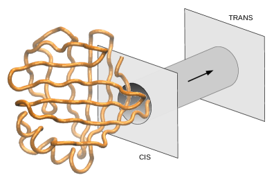
Figure 1: Cartoon of the setup employed in our molecular dynamic simulations. The LPB backbone chain extracted from the file 2MM3.pdb Horváth et al. (2016) is prepared at the channel entrance, vertical walls represent the membrane whose impenetrability is guaranteed by the repulsive force $\{F_{w}(x),0,0\}$ normal to the walls. The arrow indicates the pulling direction from CIS to TRANS side.

A repulsive force, $F_{w}(x)$, orthogonal to planes $x=0$, $x=L$ and vanishing for $y^{2}+z^{2}<R_{p}^{2}$, mimics the presence of the impenetrable membrane where the pore is inserted in

$$F_{w}(x)=\begin{cases}-\dfrac{e^{\lambda x}}{x+c}&x\leq 0\\ 0&0<x<L\\ \dfrac{e^{-\lambda(x-L)}}{x-L+c}&x\geq L\end{cases}$$

with $c=10^{-4}\AA$ being a regularisation cutoff to avoid overflow near the walls. In this work, we choose $\alpha=3$ and amplitude $\delta=0.3$. The pore length $L=100\AA$ and radius $R_{0}=10\AA$ are taken from $\alpha$HL structural data Song et al. (1996). Since $R_{0}$ is smaller than the gyration radius of the folded LBP structure, full translocations imply partial or complete unfolding. For facilitating the entrance of the chain into the nanopore, an inert linker of five extra beads was added to the N-terminus of the LPB, this linker extends the free tail protruding from the globule that has to be pulled. The importing mechanism that drives the protein into the pore is simplified to a constant pulling force $(F,0,0)$ acting only on the N-terminus bead ($\mathbf{r}_{N}$) in such a way that the pulled terminus is constrained to slide along the pore axis for all time, i.e., $y_{N}(t)=z_{N}(t)=0$.

III Results

We import the LBP from left to right inside the pore, and simulations are run until the whole chain lies outside the channel, on the cis-side. The initial conformation of each translocation run is obtained by equilibrating the chain at code temperature $T=0.3$ ($T\simeq 150^{o}$K) and $F=0$, while the pulling terminus is kept at the position ${x_{N}=-1,y_{N}=0,z_{N}=0}$, near the entrance of the static pore ($\omega=\delta=0$). Once the translocation run is completed, a new run is restarted from a different thermalised initial condition, the procedure is repeated until a robust statistics of translocation events is collected. Even for a coarse-grained description of the protein dynamics, the conformation space is still very high-dimensional to allow a concise representation of the translocation. It is thus convenient to “project” the system trajectories onto an effective (or collective) coordinate that is a function of the aminoacid positions. A suitable choice suggested by Polson et al. Polson and McCaffrey (2013) is the collective variable

$$Q=\frac{1}{N}\sum_{i=1}^{N}g(x_{i})\,$$ (3)

defined by the piecewise function

$$g(x)=\begin{cases}0&\mbox{if\leavevmode\nobreak\ }x<0\\ x/L&\mbox{if\leavevmode\nobreak\ }0\leq x<L\\ 1&\mbox{if\leavevmode\nobreak\ }x\geq 1\end{cases}$$

The value $Q=0$ corresponds to the whole protein on the cis-side, while $Q=1$ to a successful translocation. Along with $Q$, we also monitor the number of LBP residues that during the translocation lie on the cis-side of the pore:

$$N_{cis}(t)=N-\sum_{i=1}^{N}\Theta(x_{i})\,,$$ (4)

$\Theta(s)$ being the unitary step function. This quantity, during a translocation event, starts from the maximal value $N_{cis}=N$ and decreases to zero. Even if $N_{cis}$ is not a good progress coordinate, as the state $N_{cis}=0$ does not entail yet completed translocation events, it allows locating the position of the stalling points along the chain because stalls manifest as plateaus in the $N_{cis}$ time course. An important physical quantity of translocation processes is the passage time, i.e. the time the molecule takes to cross the pore. If we assume that the LBP is prepared at $t=0$ on the pore entrance (CIS-side), the first-passage time is the first time at which the molecule lies outside the pore exit (TRANS-side), and it can be easily defined in terms of $Q$:

$$t_{\mathrm{FP}}=\min_{0<t\leq T_{w}}\{t\;|\;Q(t)=1\}$$

where $T_{w}$ is the observation time window. As the statistics of $t_{\mathrm{FP}}$ can be easily measured in experiments, it is important to predict the dependence of $t_{\mathrm{FP}}$ on the system parameters such as the: chain length, type of driving force, pore fluctuations etc. A reference theoretical framework for the statistical analysis of $t_{\mathrm{FP}}$ assumes $Q$ to be a random process governed by a driven Brownian motion Lubensky and Nelson (1999); Berezhkovskii and Gopich (2003); Muthukumar (2011); Ammenti et al. (2009)

$$\dot{Q}=\mu_{0}F+\sqrt{2D_{0}}\;\xi(t)$$ (5)

where $\mu_{0}F$ accounts for average drift determined by the pulling mechanism and $\sqrt{2D_{0}}\;\xi(t)$ embodies both thermal and environment fluctuations. A successful translocation event requires that a trajectory of $Q(t)$ is released at $Q(0)=0$ (cis) and terminated when $Q(t)=1$, (trans). The statistics of $t_{\mathrm{FP}}$ associated with Eq.(5) is well known since the works by Schrödinger and Smoluchovski Schrödinger (1915); Smoluchowski (1915); Redner (2001) and it is characterized by the Inverse Gaussian distribution Chhikara (1988). However for practical purposes explained below, it is more convenient to employ the cumulative distribution function (CDF) of the Inverse Gaussian, that reads

$$F_{IG}(t)=\dfrac{1}{2}\bigg{\{}\phi\left(\dfrac{L-\mu_{0}Ft}{2\sqrt{D_{0}t}}\right)+\mbox{e}^{\mu_{0}FL/D_{0}}\phi\left(\dfrac{L+\mu_{0}Ft}{2\sqrt{D_{0}t}}\right)\bigg{\}}$$

where $\phi(u)=\mbox{Erfc}(u)$ is the complementary error function Arfken et al. (2011).

III.1 Static pore

We begin our analysis from the case of a static pore, $\delta=\omega=0$, when the translocation dynamics of the LPB presents the interesting feature of a stalled event, for which the translocation progress is not uniform in time, but gets jammed when certain chain segments approach the pore entrance. These stalling points are associated with specific LBP conformations that are particularly difficult to be unravelled. To some extent, they behave as “temporary knots” of the chain Szymczak (2016, 2014); Huang and Makarov (2008) contributing to a remarkable transport slowdown. Stalling events that are particularly persistent are to be considered intermediates of translocation, as they are statistically robust to imprint an unmistakable multistep signature on observables in experiments Talaga and Li (2009); Rodriguez-Larrea and Bayley (2013); Maillard et al. (2011); Sen et al. (2013); Nivala et al. (2013) and simulations Tian and Andricioaei (2005); Bacci et al. (2012, 2013); Bonome et al. (2015)

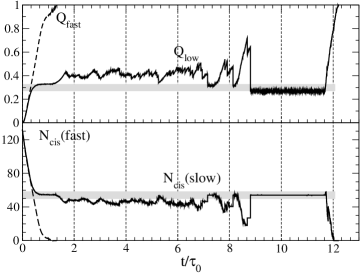
Figure 2: Time course of $\langle N_{cis}(t)\rangle_{S,F}$ and $\langle Q(t)\rangle_{S,F}$ where subscripts denote that the averages are restricted to the ensemble of fast and slow translocations for a total of $M=3600$ independent runs. Slow translocations are characterised by intermediates (stalls) that contribute with a noisy plateau to the mean time behaviour (gray bands). In the lower panel, the value $\langle N_{cis}(t)\rangle_{S}\simeq 54$ indicates a stalling point of the LPB due to a persistence of the intra-chain interactions that stabilise the block of strands S1 (4–12), S2 (46–53) and S3 (46–53), see Fig. 4.

We run $M=3600$ successful LPB translocations, each with a duration $t_{m}$, leading to a mean translocation time $\tau_{0}=\sum_{m=1}^{M}t_{m}/M=8279.2\,t_{u}=21525.9\,$ps. In the following, the time will be rescaled with $\tau_{0}$. In such simulations, the signature of a stalled dynamics turns to be evident by looking at the time behaviour of the two averages $\langle Q(t)\rangle$ and $\langle N_{cis}(t)\rangle$ taken over an ensemble Fig.2. Both indicators show early variations which are then followed by long stationary phases before reaching their absorbing state ($N_{cis}=0,Q=1$). To analyse separately the short and long time behaviours, it is convenient to split $\langle Q(t)\rangle$ and $\langle N_{cis}(t)\rangle$ in fast and slow components. We define slow translocations those which are completed in a time $t>T_{cut}=1.08\times 10^{4}t_{u}$. While the fast components (dashed lines) saturate soon to the expected values in a monotonic way, the slow components follow the fast ones for a while, then deviate toward a flat stationary noisy behaviour corresponding to the stalled state with $N_{cis}\simeq 54$. We compute the fraction of time the LPB chain spends in a state with a given $N_{cis}$, this quantity is defined by the histogram

$$H(N_{cis})=\dfrac{1}{T_{M}}\sum_{m=1}^{M}\int_{0}^{t_{m}}\!dt\;\delta[N_{cis}-N_{cis}(t)]$$

where the sum runs over the $M$ translocations and $T_{M}=\sum_{m=1}^{M}t_{m}=M\tau_{0}$. Likewise, we split $H(N_{cis})$ into fast and slow components, Fig.3. The histogram of fast events is practically flat indicating that each chain conformation is uniformly visited. On the contrary, the slow component presents a narrow and pronounced peak emerging from the background in $N_{cis}=54$, confirming that the LBP chain spends a relevant amount of time in the state with the bead $54$ at the pore entrance.

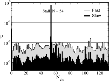
Figure 3: Visiting frequency (histogram) of states $N_{cis}$ during each translocation run. The occurrence frequency is split into “fast” and “slow” components as it is computed over fast and slow translocation sets.

With reference to the LBP native structure topology, Fig. 4, one can deduce that stalling at site $54$ lies just after the end of S3 (segment 46–53), suggesting that S3 along with two other strands, S1 (segment 4–12) and S2 (segment 36–43) form a block that is structurally robust, likely involving also the participations of the two helices A2 (13–22), A2 (25–35). The persistence of such a block causes the jamming of the protein moreover, it often squeezes into the pore and translocates as a single unit. In other translocation runs, instead, the block breaks down allowing a true single-file passage of the molecule.

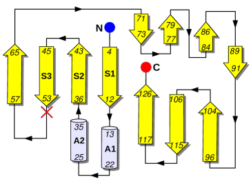
Figure 4: Topology of the LBP native structure, arrows and cylinders represent strands and helices, respectively. The red cross marks the stalling site, 54, located just after the end of strand S3 (46–53), that with strands S1 (4–12), S2 (36–43) forms the core of a stable block, weakly involving helices A2 (13–22), A2 (25–35). The protein is pulled from the C-terminus (Red dot).

To complete the characterization of the LPB translocation dynamics, we analyzed the statistics of translocation time by computing the empirical CDF over a sample of $M$ successful translocations occurred at times $\{t_{1},\ldots,t_{M}\}$,

$$F_{M}(t)=\dfrac{1}{M}\sum_{k=1}^{M}\theta(t-t_{k})\;,$$

where $\theta(s)$ denotes the unitary step function. The advantage of the CDF over the histogram lies in its independence of binning, so it is not affected by the chosen discretization. Fig.5 displays the comparison between the expected and the empirical CDF for LPB translocations.

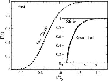
Figure 5: Empirical CDF, $F_{M}(t)$, of translocation times associated to fast events (dots) compared with $F_{IG}(t)$ (dashed line). Parameters $D_{0}=1.56\times 10^{-6}$ and $\mu_{0}=6.9\times 10^{-5}$ are obtained by the Maximum Likelihood values of the Inverse Gaussian, Eqs.(6). Inset: Empirical CDF of the translocation times of slow events characterized by stalls. Points are the simulation data and dashed line is the CDF of an exponential distribution with $\lambda=7.3\times 10^{-5}$ and $T_{cut}\simeq 1.08\times 10^{4}$.

The values of parameters $D_{0}$ and $\mu_{0}$ have been obtained from the maximum likelihood estimation (MLE),

$$\mu_{0}=\dfrac{1}{F\langle t\rangle}\quad,\quad D_{0}=\frac{1}{2}\bigg{(}\left\langle\dfrac{1}{t}\right\rangle-\dfrac{1}{\langle t\rangle}\bigg{)}$$ (6)

where angular brackets stand for the arithmetic average over $M$ independent realizations $\langle x\rangle=(x_{1}+x_{2}\cdots+x_{M})/M$. The inset of Fig.5 shows the empirical CDF of slow translocations that is consistent with the CDF = $1-\exp[-\lambda(t-T_{cut})]$ of an exponential probabilistic law. In conclusion, the comparison of the CDFs indicates fast translocations contribute to the Inverse Gaussian bulk of the time distribution, whereas, few slow translocations are responsible for the slow exponential decay of the long-time tail. In the next section, we study how the above transport scenario characterised by stalling points is modified when the pore section undergoes periodic fluctuations.

III.2 Oscillating pore

We repeated the translocation runs at different frequencies $\omega$ of the radius modulation to assess how the pore dynamics affects both the LBP mechanical denaturation and the subsequent transport. In particular, it is interesting to analyse the robustness of RA scenario Pizzolato et al. (2010); Park and Sung (1998); Ikonen et al. (2012); Cohen et al. (2011) when translocation dynamics is affected by the presence of extreme events like stalls. We begin by plotting in Fig.6 the dependence of the mean translocation time $\tau$ on the frequency of pore vibration. Data are rescaled with the static mean translocation time, $\tau_{0}=21525.9\,$ps, i.e. $\tau/\tau_{0}$ vs. $\omega\tau_{0}$. The horizontal lines mark the translocation time for the static pore with radius: $R_{max}=13\AA$, $R_{0}=10\AA$, for a comparison. We observe different translocation regimes (labelled A,B,C) resulting in a non monotonic behaviour of translocation time versus the forcing frequency, in analogy with translocation of structureless polymers Pizzolato et al. (2013); Ikonen et al. (2012); Cohen et al. (2011). In region A ($\omega\tau_{0}<10^{-2}$), the average translocation time is close to, but larger than, the static value, $\tau(\omega)>\tau_{0}$, indicating a moderate slowing down of translocations with respect to the still pore.

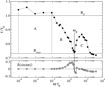
Figure 6: Upper panel: Dependence of the mean translocation time $\tau$ on the frequency at a force $F=2.0\,f_{u}=27.46\,$pN. Rescaling with $\tau_{0}$ makes data dimensionless. Three translocations regimes can be identified corresponding to regions A, B, C in the $\omega$-range. A part from region A, the RBM of the pore generally reduces the translocation time and the transport across the nanopore is speeded up by oscillations. Lower panel shows the behaviour of Eq.(10) as a function of the rescaled $\omega$. The first value at which $\langle\sin(\omega\tau)\rangle=0$, marked by the thick vertical line, identifies the resonant frequency $\omega_{R}$ at which $\tau(\omega)$ attains its minimum.

In the intermediate regime ($10^{-2}<\omega\tau<\omega_{R}\tau_{0}$), region B, $\tau(\omega)<\tau_{0}$ and it decreases with $\omega$. In this range, vibrations speed up the transport dynamics with respect to the static case moreover, the acceleration improves by increasing $\omega$ till reaches an optimal value at $\omega_{R}\tau_{0}$. Finally, in regime C, $\tau(\omega)$ attains a maximum which yet lies below $\tau_{0}$, whereby translocations result to be still improved by the RBM dynamics. To verify that the plot of Fig.6 is consistent with RA Doering and Gadoua (1992), we studied the two-state dynamics defined by the Langevin equation

$$\dot{Q}=\mu_{0}F-\mu_{0}\dfrac{\partial V}{\partial Q}+\sqrt{2D_{0}}\xi(t)\,,$$ (7)

obtained by adding to Eq.(5) a force term derived from the time dependent potential

$$V(Q,t)=\dfrac{V_{0}\,f(\omega t)}{4}\;Q^{2}(Q-1)^{2}$$ (8)

which represents a “caricature” of a translocation free-energy landscape where, presumably, a barrier separates two minima: $Q=0$ (cis) and $Q=1$ (trans). The amplitude $V_{0}$ is multiplied by

$$f(\omega t)=1+h\sin(\omega t+\phi)$$ (9)

to account for barrier oscillations $V_{b}(t)=V_{0}\,f(\omega t)/64$. The phase $\phi$ is an extra parameter necessary to fit the model to the pore RBM: opening translates into barrier lowering, while, pore shrinking corresponds to increasing the barrier. We integrated numerically Eq.(7) via a second order stochastic Runge-Kutta algorithm Honeycutt (1992) and computed the average first-arrival time to the state $Q=1$ from $Q(0)=0$, over a set of $10^{4}$ trajectories. Fig.7 shows the mean first-arrival time as a function of $\omega$. The qualitative similarity between plots in Fig.7 and Fig.6 suggests that RA is verified and that translocation of the LPB across a vibrating channel can be idealised as a transition to an absorbing state over an oscillating barrier.

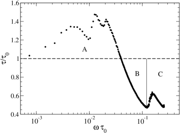
Figure 7: Two-state model with a fluctuating barrier. First arrival time of trajectories started at $Q=0$ and absorbed at $Q=1$, obtained by a numerical integration of Eq.(7) with parameters $D_{0}=1$, $F=0.001$, $V_{0}=8\times 64$, $h=0.3$, and $\phi=0$. Plot and frequency regions A,B,C are consistent with Fig.6.

Both plots in agreement with RA exhibit a minimum of $\tau(\omega)$ at a certain “resonant” or “optimal” frequency $\omega_{R}$, separating regions A and B, at which the fastest translocations are expected to be observed. A simple physical argument suggests that LPB translocations are greatly favoured as long as they are completed in a time interval $\Delta t$ such that the pore stays “open”: $R_{0}[1+\delta\sin(\omega\Delta t)]>R_{0}$, corresponding to the inequality, $0<\omega\Delta t<\pi$. Therefore, the optimal frequency $\omega_{R}$ at which translocations are faster is bounded in the range, $\omega_{0}/2<\omega_{R}<\pi/\tau(R_{max})$, where $\tau(R_{max})$ denotes the mean translocation for a static pore at maximal radius $R_{max}=R_{0}(1+\delta)$, indicated by the lowest horizontal line in Fig.6. To verify this conclusion, in the lower panel of the same figure, we report the average

$$\delta\langle\sin(\omega t)\rangle=\frac{1}{M}\sum_{i=1}^{M}\frac{R(t_{i})-R_{0}}{R_{0}}\;,$$ (10)

over $M$ translocation times $t_{i}$, estimating the typical radius oscillation at the end of translocations at each $\omega$. It is apparent that by following the bold vertical line, that the first zero of $\langle\sin(\omega t)\rangle$ coincides with the resonant frequency $\omega_{R}$ at which $\tau(\omega)$ attains its minimum. This confirms that at the resonant condition, $\omega_{R}\tau\simeq\pi$, luckiest translocations occurs in the half-cycle of the RBM, in which the pore offers minimal hindrance to the transport. It is instructive to gain further insight into the physics of RA by adapting to our case the phenomenological approach to stochastic resonance by McNamara and Wiesenfeld McNamara and Wiesenfeld (1989). It amounts to writing a rate equation for the activated kinetics of model (7) with the help of the well-known Kramers formula Kramers (1940)

$$k=\dfrac{\Omega_{0}\Omega_{b}}{2\pi\gamma}\exp\{-\beta V_{b}\}\;.$$

Where $\gamma$ is the solvent viscosity, $\Omega_{0},\Omega_{b}$, the angular frequencies (curvatures) at the bottom and at the top of the barrier of the tilted potential, $W(Q,t)=V(Q,t)-FQ$. As it is shown in Appendix A, Kramers theory gives, for a weak external field $F$, the rate expression

$$k(\omega t)\simeq ae^{-\epsilon\sin(\omega t+\phi)}[1+c\sin(\omega t+\phi)];\qquad(\epsilon=\beta V_{0}h/64)$$ (11)

to the first order in $F/V_{0}$. The constant $c$ and the factor $a$ are defined in the appendix. Eq.(11) represents the lowest term of a Kramers escape-rate modulated by a unimodal potential vibration, high order terms in the expansion contribute with higher harmonics. This analytical approach remains physically meaningful as long as barrier oscillations are not too fast (adiabatic regime) with respect to the relaxation dynamics in the well: the adiabatic regime requires $\omega\ll\Omega_{0}$, a condition certainly verified by the case in Fig.7. The rate-theory in appendix A shows that Eq.(11) leads to the analytical expression

$$\tau(\omega)=\dfrac{{\displaystyle\int_{0}^{2\pi}}\!\!dx\;\exp\{-Y(x)/\omega\}}{\omega\big{[}1-\exp(\,-2\pi\;k_{\mathrm{eff}}/\omega\,)\big{]}}$$ (12)

for the average translocation time, with

$$Y(x)=\int_{0}^{x}\!\!du\;k(u)\;.$$

being the integral of the rate (11) and

$$k_{\mathrm{eff}}=\dfrac{1}{T}\int_{0}^{T}\!\!dt\;k(\omega t)=\dfrac{Y(2\pi)}{2\pi}$$ (13)

being the average rate over a period of vibration. The resonant frequency $\omega_{R}$ is the minimum of $\tau(\omega)$. As discussed in Appendix A, this minimum is close to the value $\omega_{*}\pi\;k_{\mathrm{eff}}$ at which the argument of the exponential at denominator in Eq.(12) equals $1/2$. At low frequency, the escape from the barrier is basically determined by the frozen value of $k(0)$ (barrier height) that is selected by the initial condition of the dynamics. Whereas at high frequency, the escape is determined by the average rate (barrier) $k_{\mathrm{eff}}$. The resonant minimum basically separates these two regimes. In summary, the basic condition for emergence of RA is an escape process modulated by a time periodic rate. It is reasonable to assume that a similar situation occurs in the LBP translocation. Now it interesting to investigate the effect of the channel fluctuations on the persistence of the stalling events. This can be achieved by measuring how much the trajectories of $N_{cis}$ experiences the influence of the pore frequency. Fig.8 reports the time course of the average $N_{cis}$ over $3600$ runs, for different values of $\omega$. We recall that $N_{cis}$ is particularly useful for identifying the stalled dynamics. From main panel of Fig.8, we observe that in the frequency range C (as defined in Fig.6), pore vibrations transfer to the translocation dynamics, indeed $\langle N_{cis}(t)\rangle$ develops an oscillating decay to zero with the pore frequency. The locking between pore and protein pulled-dynamics is expected, because if the pore is maximally closed, the protein dynamics is hindered and temporary stalled. In that condition, $N_{cis}$ statistically assumes the same value, leading to equally spaced peaks in the plots. However, the decay without oscillations shown by the red-dashed curve, obtained at a frequency just below the region C, proves that such a frequency locking is restricted to the frequency region C. The oscillation of the thick-black curve, corresponding to a frequency just above region C, is almost imperceptible because the protein dynamics is becoming not responding to such fast pore oscillations. However, it should be remarked that the absence of an evident frequency locking does not imply a translocation dynamics which is not sensitive to the forcing applied by the pore. Indeed, the plots of $\langle N_{cis}(t)\rangle$ in the inset of Fig.8 show that the duration of the stalls soon reduces as the pore vibrates even at low frequency, and by increasing $\omega$ the duration is further decreased till vanishing above a certain frequency threshold. We stress that time shortening of stalls does not necessarily imply an average speeding up of translocations, in particular, region A of Fig.6 is just characterised by translocations with $\tau(\omega)>\tau_{0}$ notwithstanding the stall depression. If stalls are regarded as extreme events, their reduction is crucial in order to regularise the translocation dynamics according to the principle that suppression of extreme events generally makes a process more predictable and controllable Cavalcante et al. (2013). The data suggest that a specific cycle of expansions and compressions of the channel may either control or even facilitate the translocation of proteins across it. The result can be summarised by the statement: “tuned RBM of a nanopore catalyses pulled translocation of globular proteins”. As shown in Refs.Szymczak (2016); Tian and Andricioaei (2005), an analogous catalytic effect can be achieved by setting the modulation on the pulling force that unfolds and translocates polypeptide chains and proteins.

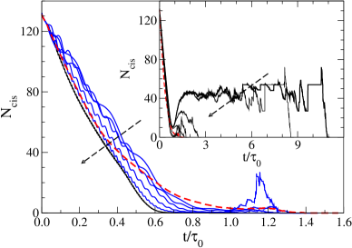
Figure 8: Main panel: modulated evolutions of $\langle N_{cis}(t)\rangle$ with the pore frequency as a consequence of the transmission of pore oscillations to translocation dynamics. This oscillating decay of $\langle N_{cis}(t)\rangle$ is well distinguishable only in the frequency range coincident with region C of Fig.6. The modulation is soon lost for frequencies just below region C, see the steady decay of the red-dashed curve, and it becomes imperceptible at frequencies just above region C, see black-thick curve. Inset shows the stall suppression in translocations at pulling $F=27.46\,$pN ($F=2.0$ code units) when increasing the oscillation frequency of the pore section, dashed arrows indicate the increase of $\omega$. It is apparent how the plateau length of $\langle N_{cis}\rangle$ reduces when $\omega$ increases, till vanishing when $\omega\to\omega_{0}$.

In the region C (Fig.6), we observe that PdF of translocation time develops a multi-peaked structure reflecting the pore cycles, see Fig.9. The minima and maxima of the PdF correspond to a maximally open and closed state of the pore respectively. Outside the region C this PdF modulation either vanishes or becomes undetectable.

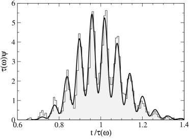
Figure 9: Comparison of the PdF of the translocation time for $\omega\sim 20\omega_{0}$ to the corresponding analytical PdF (16) with parameters $\mu_{0}=7.33\times 10^{-5}$, $D_{0}\sim 1.012\times 10^{-6}$, $h=0.60$ and $\phi=-10$.

Again a simple approach that can explain the multi-peaked structure of the translocation time PdF is bases on a First Passage Theory (FPTh) for a biased diffusion of $Q$ described by the Smoluchowski equation

$$\frac{\partial P}{\partial t}=-\mu_{0}F\frac{\partial P}{\partial Q}+D_{0}f(\omega t)\frac{\partial^{2}P}{\partial Q^{2}}$$ (14)

where $f(\omega t)$ is defined in Eq.(9), $\mu_{0}$ and $D_{0}$ denote static mobility and diffusivity respectively. In Eq.(14) instead of taking a periodic pulling force, as done in other contexts Ikonen et al. (2012); Fiasconaro et al. (2015), we preferred to consider a systematic drift $\mu_{0}F$, while shifting the modulation to the diffusion coefficient $D_{0}f(\omega t)$. This approach is more consistent with the coarse-grained molecular model implemented in our simulations and described in sect.II, where the sinusoidal oscillation of the pore applies cyclic transversal compressions on the passing chain leading to a kind of “freezing” on the transversal degrees of freedom. This has been roughly taken into account by a noise with an oscillating variance. The solution to Eq.(14) is specified by initial $P(Q,0)=\delta(Q)$ and boundary conditions,

$$J(0,t) = \mu_{0}FP(0,t)-D_{0}f(\omega t)\dfrac{\partial P}{\partial_{Q}}\bigg{|}_{0}=0$$

$$P(1,t) = 0\,;$$

the first equation is a no-flux condition which guarantees that $Q(t)$ cannot be less than zero, by definition. The second prescribes that trajectories are absorbed as soon as $Q(t)=1$. The fundamental quantity in the FPTh is the survival probability of $Q(t)$

$$S(t)=\int_{0}^{1}\!\!dQP(Q,t)$$

where $P(Q,t)$ is the solution of Eq.(14) satisfying both boundary and initial conditions. $S(t)$ is the probability that at time $t$ the process $Q(t)$ is not yet absorbed by the boundary $Q=1$, accordingly, $1-S(t)$ is the probability that $Q(t)$ exits $[0,1]$. Hence, the exit time distribution is $\psi(t)=d(1-S(t))/dt$, that is

$$\psi(t)=-\dfrac{dS}{dt}=-\int_{0}^{1}\!\!dQ\dfrac{\partial P(Q,t)}{\partial t}$$

Using Eq.(14), we obtain that $\psi(t)$ is related to probability flux evaluated at the boundary, $Q=1$,

$$\psi(t)=J(1,t)=D_{0}f(\omega t)\dfrac{\partial P}{\partial Q}\bigg{|}_{Q=1}$$ (15)

therefore, the final result reads

$$\psi(t)=\frac{1+h\cos(\omega t+\phi)}{\sqrt{4D_{0}\Delta^{3}(t)}}\exp\bigg{\{}-\frac{(1-\mu_{0}Ft)^{2}}{4D_{0}\Delta(t)}\bigg{\}}\;.$$ (16)

where $\Delta(t)=t-(h/\omega)[\cos(\omega t+\phi)-\cos(\phi)]$ is obtained by integrating $f(\omega t)$ over time, (see Eq.(27)). The derivation of this theoretical distribution is outlined in Appendix B by using the method of images to fulfil the boundary conditions. However, it is important to warn that formula (16) constitutes only a reasonable approximation of the true solution, indeed as it discussed by Molini et al. Molini et al. (2011) and in Appendix B, the image method to work, when applied to Smoluchowski equations with time dependent coefficients, requires a rigorous proportionality between drift and diffusion; a condition which is not verified in Eq.(14). In addition, we assumed the further simplification of strong enough drift that soon pushes the trajectories away from the $Q=0$-boundary, so that the no-flux condition is automatically implemented. Despite the approximation, formula (16) can be considered a good fitting model, that, upon tuning the parameters $\mu_{0},D_{0},h,\phi$, is able to reproduce and explain quite naturally the essential features of the simulated PdF, including the peculiar peaked structure as shown in Fig.9, where the function (16) fits well the histogram of LBP translocation times.

IV Conclusions

We investigated the translocation process of a protein in the family of Lipid Binding Proteins across a nanopore via a coarse-grained molecular dynamic simulations that simplify both pore and chain. In our phenomenological model, the protein is described as a chain of beads interacting via a Gō-like force field which is known to guarantee the correct formation of the secondary structure by rewarding those interactions that stabilise the geometry of the native state. The presence of a constant driving force mimics the average effect of the biological importing mechanism into a nanopore (cylinder) whose cross section varies periodically in time simulating the effect of a radial breathing mode (RBM) induced by a cyclically varying environment. Our study differs from previous ones Pizzolato et al. (2013); Ikonen et al. (2012); Fiasconaro et al. (2015); Cohen et al. (2011); Mondal and Muthukumar (2016); Zhang et al. (2012); Cohen et al. (2012) that focused on bead-spring polymers, for it investigates the translocation of a protein-like chain. The translocation of proteins is known to strongly deviates from that of polymers as their compactness presents much more resistance to the passage through narrow paths. This important feature, generally known as “structure-dependent translocation”, makes the transport of proteins in nanopores a complex phenomenon still difficult to be both modelled and predicted. The Lipid Binding Protein (LBP) does not make an exception. Indeed, our MD simulations of its pulled translocation into a static pore, performed by the coarse-grained model, exhibit the typical intermittency of a process that is dominated by few extreme stalled events. More specifically, the chain gets temporarily stuck in metastable conformations that are hardly unravelled and depend on the LBP’s arrangement in its own native state. We repeated the same simulations with a pore undergoing a radial vibration (radial breathing mode (RBM)) to study the dependence of the average translocation time $\tau$ on the RBM frequency $\omega$. The comparison with the static case proved that the RBM reduces the duration of stalling events until it makes them disappear above a certain frequency threshold. It is interesting to note that there exists a low frequency range, where the translocation process is slowed down by the RBM of the pore, despite a reduction of the stalling periods. The suppression of stalling duration, even if does not always bring to an accelerated transport, is crucial to “regularise” the process by suppressing extreme events. In other regimes, a frequency locking occurs between the RBM and translocation dynamics; the translocation observable develops oscillations with the pore frequency and the distributions of translocation time show a succession of peaks strictly reflecting such a locking.

V Acknowledgements

The authors warmly thank A. Cavagna, R. Larciprete, M. Chinappi and L. Pilozzi for very useful discussions and their valuable suggestions.

Appendix A Rate equation

In this appendix we derive the escape rate (12) by applying the Kramers’ theory to the tilted bistable potential (8)

$$W(Q,t)=\frac{A(t)}{4}Q^{2}(Q-1)^{2}-FQ\;.$$ (17)

According to Kramers Kramers (1940), the rate at which a Brownian dynamics leaves the left well of $W(Q,t)$ upon crossing the barrier reads

$$k=\dfrac{\sqrt{W^{\prime\prime}(Q_{0})\;|W^{\prime\prime}(Q_{b})|}}{2\pi\gamma}\exp\{-\beta V_{b}\}.$$

where $\beta=(k_{B}T)^{-1}$, $\gamma$ is the solvent viscosity, $W^{\prime\prime}(Q_{0})$ and $W^{\prime\prime}(Q_{b})$ are the second derivatives of the potential (17) evaluated at the bottom of the well $Q_{0}$ and at the top of the barrier $Q_{b}$, respectively. Even in this simple framework, the rate formula becomes quite involved for a full analytical approach. The expression simplifies considerably in the limit of a weak field by retaining terms to the first order in $F/A$. The weak field shifts the well and barrier from the unperturbed positions $Q_{0}=0,Q_{b}=1/2$ to $Q_{0}\simeq 2(F/A)$, $Q_{b}\simeq 1/2-4(F/A)$, moreover it decreases the barrier height from $V_{b}=A/64\to A/64-0.5(F/A)$. A further expansion of $k$ in $F/A$ yields the result

$$k(\omega t)\sim a\dfrac{1+c\sin(\omega t+\phi)}{\tau_{0}}e^{-\epsilon\sin(\omega t+\phi)}$$ (18)

with constants $c=h/(1-6F/V_{0})$, $\epsilon=\beta V_{0}h/64$, and

$$\tau_{0}=\dfrac{4\pi\;\gamma\;\sqrt{2}}{V_{0}-6F}\;e^{\beta(V_{0}/64-F/2)}$$

being the static escape time in the Kramers approximation. As a consequence of barrier oscillations, the rate $k(\omega t)$ turns to be a periodic functions with period $T=2\pi/\omega$. The factor $a=\tau_{0}^{-1}\exp[\epsilon\sin(\phi)]/[1+c\sin(\phi)]$ ensures that the limit $\omega\to 0$ recovers the static value $k(0)=1/\tau_{0}$. The kinetics of barrier crossing in the oscillating potential (8) can be described by the rate equation

$$\dfrac{dS}{dt}=-k(\omega t)S\,,$$ (19)

for the probability $S(t)$ that at time $t$ the process still occupies $Q_{0}$ well, $S(t)$ is also called the survival probability of $Q_{0}$-state. In the formulation of our problem, Eq.(19) contains only the loss contribution, as the molecule is removed after each successful translocation and re-injected from the CIS-side (impossibility of back-transitions). Integration of Eq.(19), with initial condition $S(0)=1$, leads to the solution

$$S(t)=\exp\bigg{\{}-\int_{0}^{t}\!du\;k(\omega u)\bigg{\}}\,,$$

which describes a decay to zero as translocation proceeds. The quantity $1-S(t)$ is the probability that a molecule has crossed the boundary at time $t$ and it is removed, so the distribution of exit times is given by $\psi(t)=-S^{\prime}(t)$, accordingly the mean exit (translocation) time is soon obtained from $\psi(t)$ and reads,

$$\tau(\omega)=\int_{0}^{\infty}\!\!dt\;S(t)=\int_{0}^{\infty}\!\dfrac{dt}{\omega}\;\exp\bigg{\{}-\int_{0}^{t}\!\dfrac{du}{\omega}\;k(u)\bigg{\}}\,,$$

after an integration by part and a change of variables. To take advantage of the periodicity of $k(u)$, the integral can be split in a series of integrals over the periods, corresponding to intervals $[2\pi n,2\pi n+2\pi]$,

$$\tau(\omega)=\dfrac{1}{\omega}\sum_{n=0}^{\infty}\;\int_{0}^{2\pi}\!\!d\xi\;\exp\bigg{\{}-\dfrac{1}{\omega}\int_{0}^{2\pi n+\xi}\!\!du\;k(u)\bigg{\}}$$

where we applied the change of variable $t=2\pi n+\xi$. Thanks to periodicity, we can refold the integration onto the cell $[0,2\pi]$ and the argument of the exponential is recast as

$$n\int_{0}^{2\pi}\!\!du\;k(u)+\int_{0}^{\xi}\!\!du\;k(u)$$

with a final result

$$\tau(\omega)=\dfrac{1}{\omega}\sum_{n=0}^{\infty}e^{-nY(2\pi)/\omega}\int_{0}^{2\pi}\!\!dt\;\exp\bigg{\{}-\dfrac{1}{\omega}\int_{0}^{t}\!\!du\;k(u)\bigg{\}}.$$

According to the formula of a geometric-series sum, it becomes

$$\tau(\omega)=\dfrac{{\displaystyle\int_{0}^{2\pi}}\!\!dx\;\exp\{-Y(x)/\omega\}}{\omega\big{(}1-\exp[-Y(2\pi)/\omega\,]\big{)}}$$ (20)

where the function $Y(x)$ is the integral of the rate (18)

$$Y(x)=\int_{0}^{x}\!\!d\xi\;k(\xi)\;,$$

and $Y(2\pi)=2\pi a[I_{0}(\epsilon)-hI_{1}(\epsilon)]$; $I_{0}(x),I_{1}(x)$ being the modified Bessel function of the First Kind for $n=0$ and $1$ respectively Arfken et al. (2005). Expression (20) has the advantage to make the $\omega$-dependence of $\tau$ explicit providing the very final expression of the average translocation time ready to be used in numeric computations and qualitative analysis. A first observation stems from the two limiting behaviours: $\omega\to 0$ (quasistatic barrier) yields $\tau(0)=\tau_{0}$, while, for $\omega$ large (fast oscillations), we have $\tau(\infty)=Y(2\pi)=2\pi k_{\mathrm{eff}}^{-1}$, where

$$k_{\mathrm{eff}}=\dfrac{e^{\epsilon\sin(\phi)}}{\tau_{0}\;[1+h\sin(\phi)]}[I_{0}(\epsilon)-hI_{1}(\epsilon)]$$ (21)

corresponds to the average of the rate (18) over one oscillation period $T$, therefore we can re-write

$$\tau(\omega)=\dfrac{\omega^{-1}}{1-\exp[-2\pi\;k_{\mathrm{eff}}/\omega]}\int_{0}^{2\pi}\!\!dx\;\exp\bigg{\{}-\dfrac{Y(x)}{\omega}\bigg{\}}$$ (22)

which is exactly Eq.(12) of Sec.III.2. The function $\tau(\omega)$ develops a minimum for a “resonant” frequency $\omega_{R}$ (see Fig.10) that can be computed by solving numerically the equation $\partial_{\omega}\tau=0$, full dots in Fig.10. However, to arrive at an analytical expression useful for qualitative analysis, we can observe that $\omega_{R}$ is close to the crossover point $\omega_{*}$ determined by the condition $2\pi\;k_{\mathrm{eff}}/\omega_{*}\simeq 1/2$ for the exponential at denominator of Eq.(22).

$$\omega_{*}=\omega_{0}\dfrac{e^{\epsilon\sin(\phi)}}{2[1+c\sin(\phi)]}[I_{0}(\epsilon)-hI_{1}(\epsilon)]\;.$$ (23)

This value can be considered a rough yet reasonable estimate of $\omega_{R}$, as it shown in Fig.10, open circles.

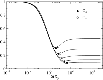
Figure 10: Plot of $\tau(\omega)$ from Eq.(22), computed for the same parameters of Fig.(7), giving $\epsilon=2.4$, at 5 values of the phase: $\phi=2.57+n\times 0.2$, $n=1,\ldots,5$. The curves clearly show the resonant minimum as expected from a RA process. Full circles mark the true minima, open circles represent the corresponding values of $\omega_{*}$, Eq.(23), which can be considered a rough estimate of the resonant frequency.

Appendix B Toy model

This appendix shows the derivation of formula (16) for the translocation time PDF. The collective coordinate $Q$ is supposed to follow the driven-diffusion dynamics Lubensky and Nelson (1999); Berezhkovskii and Gopich (2003); Muthukumar (2011); Ammenti et al. (2009)

$$\dot{Q}=\mu_{0}F+\sqrt{2D_{0}}\;\eta(t)$$ (24)

$\eta$ indicates a Gaussian noise, with $\langle\eta(t)\rangle=0$ and autocorrelation $\langle\eta(t)\eta(s)\rangle=f(\omega t)\,\delta(t-s)$ according to Eq.(9), and $\mu_{0},D_{0}$ are the mobility and diffusivity of $Q$ when $f(\omega t)=1$, respectively. The solution to the stochastic differential Eq.(24) with initial condition $Q(0)=0$ is

$$Q(t)=\mu_{0}Ft+\sqrt{2D_{0}}\int_{0}^{t}\!\!ds\;\eta(s)$$ (25)

it defines a Gaussian process with average and spreading

$$\langle Q(t)\rangle=\mu_{0}Ft$$ (26)

$$\langle\,[Q(t)-\langle Q(t)\rangle]^{2}\,\rangle=2D_{0}\Delta(t)$$

where thanks to the $\delta$-correlation property of the noise, we have

$$\Delta(t)=\int_{0}^{t}\!\!ds\;f(\omega s).$$ (27)

From the solution (25), it is easy to derive the coefficients

$$\lim_{h\to 0}\;\dfrac{\langle Q(t+h)-Q(t)\rangle}{h}=\mu_{0}F$$ (28)

$$\lim_{h\to 0}\;\dfrac{\langle\,[Q(t+h)-Q(t)]^{2}\,\rangle}{2h}=D_{0}f(\omega t)$$

of the corresponding Smoluchowski equation

$$\frac{\partial P}{\partial t}=-\mu_{0}F\frac{\partial P}{\partial Q}+D_{0}f(\omega t)\frac{\partial^{2}P}{\partial Q^{2}}\,,$$ (29)

which admits the fundamental solution

$$G(Q,t)=\frac{1}{\sqrt{4\pi D_{0}\Delta(t)}}\exp\bigg{\{}-\frac{(Q-\mu_{0}Ft)^{2}}{4D_{0}\Delta(t)}\bigg{\}}$$

satisfying the initial conditions $G(Q,0)=\delta(Q)$. $G(Q,t)$ is easily obtained via the change of variables $\xi=Q-\mu_{0}Ft$ and $\tau=\Delta(t)$ that transforms Eq.(29) into an equation with constant diffusivity, no drift but same initial condition. As discussed in sec.III.2, the PdF of translocation times can be derived from the First Passage Theory (FPTh) of the process $Q(t)$ by assuming an initial condition $P(Q,0)=\delta(Q)$, a no-flux boundary at $Q=0$, $J(0,t)=[\mu_{0}FP-D_{0}f(\omega t)\partial_{Q}P]_{0}=0$ and an absorbing boundary at $Q=1$, $P(1,t)=0$. The exact solution to this problem is not available as it is not separable, in addition, the boundaries introduce further complications. However, a meaningful approximation can still be obtained by assuming that the drift is strong enough to induce a swift displacement of the process from the $0$-boundary, hence, the effect of the impenetrable barrier at $Q=0$ becomes negligible and, in a first approximation, it can be shifted to $Q=-\infty$. The other boundary instead is fulfilled trying to “extend” the method of images to the case of time-dependent diffusion coefficients as shown in Ref.Molini et al. (2011). Accordingly, we attempt the solution

$$P(Q,t)\simeq G(Q,t)-wG(Q-2,t)$$ (30)

originated from the new initial condition $P(Q,0)=\delta(Q)+w\delta(Q-2)$, where the extra term represents an auxiliary symmetric source (the image) with respect the boundary $Q=1$. The coefficient $w$ is to be determined by imposing the boundary condition $P(1,t)=0$ and leading to $w=G(1,t)/G(-1,t)=\exp\{\mu_{0}Ft/[D_{0}\Delta(t)]\}$. In Eq.(30) we did not use the “=” to stress that it is only a “pseudo”-solution, this can be verified immediately by plugging it back to Eq.(29). When the approximate solution $P(Q,t)$ is plugged into Eq.(15) and in the following ones we obtain the final analytical form (16) for the translocation time PdF. Since the theoretical distribution (16) is not exact for the model (24), it is important to test its accuracy against the true PdF of exit times that can be computed by a direct numerical integration of Eq.(24). Fig.11 shows the reasonable match of $\psi(t)$ with the histogram of first exit times from the boundary $Q=1$, obtained by a numerical integration of Eq.(24). The different curves show that the accuracy is improved by choosing an optimal value of $h$.

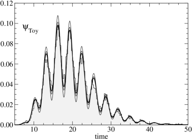
Figure 11: Test of toy model: comparison of the translocation time PdF Shaded region is the histogram of the First Exit Time form the boundary $Q=1$ with the corresponding theoretical PdF (16) from the simple driven-diffusion model of parameters: $\mu_{0}=1,D_{0}=1,F=0.05$, $h=0.60$ and $\phi=0$. The different lines represent plots of (16) at different values of $h$ showing that this parameter can be adjusted to obtain an optimal match of the approximated theory and simulations data.

References

- Schatz and Dobberstein (1996) G. Schatz and B. Dobberstein, Science, 1996, 271, 1519–1526.
- Maillard et al. (2011) R. Maillard, G. Chistol, M. Sen, M. Righini, J. Tan, C. M. Kaiser, C. Hodges, A. Martin and C. Bustamante, Cell, 2011, 145, 459–469.
- Menais et al. (2016) T. Menais, S. Mossa and A. Buhot, Sci. Rep, 2016, 6, 38558.
- Fologea et al. (2005) D. Fologea, J. Uplinger, B. Thomas, D. S. McNabb and J. Li, Nano Lett., 2005, 5, 1734–1737.
- Harrell et al. (2006) C. C. Harrell, Y. Choi, L. P. Horne, L. A. Baker, Z. S. Siwy and C. R. Martin, Langmuir, 2006, 22, 10837–10843.
- Hulea et al. (2005) I. Hulea, A. Pronin and H. Brom, Appl. Phys. Lett., 2005, 86, 252107.
- Shi et al. (1995) X. Shi, R. W. Hammond and M. D. Morris, Anal. Chem., 1995, 67, 3219–3222.
- Fanzio et al. (2012) P. Fanzio, C. Manneschi, E. Angeli, V. Mussi, G. Firpo, L. Ceseracciu, L. Repetto and U. Valbusa, Sci. Rep., 2012, 2, 791.
- Huh et al. (2007) D. Huh, K. Mills, X. Zhu, M. A. Burns, M. D. Thouless and S. Takayama, Nat. Mat., 2007, 6, 424–428.
- Ikonen et al. (2012) T. Ikonen, J. Shin, W. Sung and T. Ala-Nissila, J. Chem. Phys., 2012, 136, 205104.
- Pizzolato et al. (2013) N. Pizzolato, A. Fiasconaro, D. P. Adorno and B. Spagnolo, J. Chem. Phys., 2013, 054902.
- Fiasconaro et al. (2015) A. Fiasconaro, J. J. Mazo and F. Falo, Phys. Rev. E, 2015, 91, 022113.
- Cohen et al. (2011) J. A. Cohen, A. Chaudhuri and R. Golestanian, Phys. Rev. Lett., 2011, 107, 238102.
- Mondal and Muthukumar (2016) D. Mondal and M. Muthukumar, J. Chem. Phys., 2016, 144, 144901.
- Zhang et al. (2012) Z. Zhang, H. Chen and Z. Hou, J. Chem. Phys., 2012, 137, 044904.
- Cohen et al. (2012) J. Cohen, A. Chaudhuri and R. Golestanian, J. Chem. Phys., 2012, 137, 204911.
- Sarabadani et al. (2015) J. Sarabadani, T. Ikonen and T. Ala-Nissila, J. Chem. Phys., 2015, 143, 074905.
- Benzi et al. (1981) R. Benzi, A. Sutera and A. Vulpiani, J. Phys. A: Math. Gen., 1981, 14, L453.
- Doering and Gadoua (1992) C. R. Doering and J. C. Gadoua, Phys. Rev. Lett., 1992, 69, 2318–2321.
- Bier and Astumian (1993) M. Bier and R. D. Astumian, Phys. Rev. Lett., 1993, 71, 1649–1652.
- Pizzolato et al. (2010) N. Pizzolato, A. Fiasconaro, D. P. Adorno and B. Spagnolo, Phys. Biol., 2010, 7, 034001.
- Maultzsch et al. (2005) J. Maultzsch, H. Telg, S. Reich and C. Thomsen, Phys. Rev. B, 2005, 72, 205438.
- Tian and Andricioaei (2005) P. Tian and I. Andricioaei, J. Mol. Biol., 2005, 350, 1017–1034.
- Rodriguez-Larrea and Bayley (2013) D. Rodriguez-Larrea and H. Bayley, Nat. Nanotech., 2013, 8, 288–295.
- Bonome et al. (2015) E. L. Bonome, R. Lepore, D. Raimondo, F. Cecconi, A. Tramontano and M. Chinappi, J. Phys. Chem. B, 2015, 119, 5815–5823.
- Di Marino et al. (2015) D. Di Marino, E. L. Bonome, A. Tramontano and M. Chinappi, J. Phys. Chem. Lett., 2015, 6, 2963–2968.
- Cressiot et al. (2014) B. Cressiot, A. Oukhaled, L. Bacri and J. Pelta, BioNanoScience, 2014, 4, 111–118.
- Bacci et al. (2012) M. Bacci, M. Chinappi, C. M. Casciola and F. Cecconi, J. Phys. Chem. B, 2012, 116, 4255–4262.
- Bacci et al. (2013) M. Bacci, M. Chinappi, C. M. Casciola and F. Cecconi, Phys. Rev. E, 2013, 88, 022712.
- Szymczak (2016) P. Szymczak, Sci. Rep., 2016, 6, 21702.
- Horváth et al. (2016) G. Horváth, A. Bencsura, A. Simon, G. P. Tochtrop, G. T. DeKoster, D. F. Covey, D. P. Cistola and O. Toke, FEBS, 2016, 283, 541–555.
- Clementi et al. (2000) C. Clementi, H. Nymeyer and J. Onuchic, J. Mol. Biol., 2000, 298, 937–953.
- Hoang and Cieplak (2000) T. X. Hoang and M. Cieplak, J. Chem. Phys., 2000, 112, 6851–6862.
- Cecconi et al. (2006) F. Cecconi, C. Guardiani and R. Livi, Biophys. J., 2006, 91, 694–704.
- Burrage et al. (2007) K. Burrage, I. Lenane and G. Lythe, SIAM J. Sci. Comput., 2007, 29, 245–264.
- Ferrenberg and Swendsen (1989) A. M. Ferrenberg and R. H. Swendsen, Phys. Rev. Lett., 1989, 63, 1195–1198.
- Arighi et al. (2003) C. N. Arighi, J. P. F. C. Rossi and J. M. Delfino, Biochemistry, 2003, 42, 7539–7551.
- Song et al. (1996) L. Song, M. R. Hobaugh, C. Shustak, S. Cheley, H. Bayley and J. E. Gouaux, Science, 1996, 274, 1859–1865.
- Polson and McCaffrey (2013) J. M. Polson and A. C. McCaffrey, J. Chem. Phys., 2013, 138, 174902.
- Lubensky and Nelson (1999) D. K. Lubensky and D. R. Nelson, Biophys. J., 1999, 77, 1824–1838.
- Berezhkovskii and Gopich (2003) A. M. Berezhkovskii and I. V. Gopich, Biophys. J., 2003, 84, 787–793.
- Muthukumar (2011) M. Muthukumar, Polymer translocation, CRC Press, 2011.
- Ammenti et al. (2009) A. Ammenti, F. Cecconi, U. Marini Bettolo Marconi and A. Vulpiani, J. Phys. Chem. B, 2009, 113, 10348.
- Schrödinger (1915) E. Schrödinger, Phys. Z., 1915, 16, 289–295.
- Smoluchowski (1915) M. v. Smoluchowski, Phys. Z., 1915, 16, 318–321.
- Redner (2001) S. Redner, A guide to first-passage processes, Cambridge University Press, Cambridge UK, 2001.
- Chhikara (1988) R. Chhikara, The Inverse Gaussian Distribution: Theory: Methodology, and Applications, CRC Press, 1988, vol. 95.
- Arfken et al. (2011) G. Arfken, H. Weber and F. Harris, Mathematical methods for physicists: a comprehensive guide, Academic press, 2011.
- Szymczak (2014) P. Szymczak, EPJ, Special Topics, 2014, 223, 1805–1812.
- Huang and Makarov (2008) L. Huang and D. E. Makarov, J. Chem. Phys., 2008, 129, 121107.
- Talaga and Li (2009) D. S. Talaga and J. Li, JACS, 2009, 131, 9287–9297.
- Maillard et al. (2011) R. A. Maillard, G. Chistol, M. Sen, M. Righini, J. Tan, C. M. Kaiser, C. Hodges, A. Martin and C. Bustamante, Cell, 2011, 145, 459–469.
- Sen et al. (2013) M. Sen, R. A. Maillard, K. Nyquist, P. Rodriguez-Aliaga, S. Presse, A. Martin and C. Bustamante, Cell, 2013, 155, 636–646.
- Nivala et al. (2013) J. Nivala, D. B. Marks and M. Akeson, Nat. Biotech., 2013, 31, 247–250.
- Park and Sung (1998) P. J. Park and W. Sung, Int. J. Bifurcation Chaos, 1998, 08, 927–931.
- Honeycutt (1992) R. L. Honeycutt, Phys. Rev. A, 1992, 45, 600.
- McNamara and Wiesenfeld (1989) B. McNamara and K. Wiesenfeld, Phys. Rev. A, 1989, 39, 4854.
- Kramers (1940) H. A. Kramers, Physica, 1940, 7, 284–304.
- Cavalcante et al. (2013) H. L. d. S. Cavalcante, M. Oriá, D. Sornette, E. Ott and D. J. Gauthier, Phys. Rev. Lett., 2013, 111, 198701.
- Molini et al. (2011) A. Molini, P. Talkner, G. G. Katul and A. Porporato, Physica A, 2011, 390, 1841–1852.
- Arfken et al. (2005) G. B. Arfken, H. J. Weber and F. Harris, Mathematical Methods For Physicists 6th ed., New York: Academic, 2005.