Non-Analytic Crossover Behavior of SU($\mathcal{N}_{c}$) Fermi Liquid

Abstract

We consider the thermodynamic potential of a dilute Fermi gas with a contact interaction, at both finite temperature $T$ and non-zero effective magnetic fields $\mathbf{H}$, and derive the equation of state analytically using second order perturbation theory. Special attention is paid to the non-analytic dependence of $\Omega$ on temperature $T$ and (effective) magnetic field $\mathbf{H}$, which exhibits a crossover behavior as the ratio of the two is continuously varied. This non-analyticity is due to the particle-hole pair excitation being always gapless and long-ranged. The non-analytic crossover found in this paper can therefore be understood as an analog of the Ginzberg-Landau critical scaling, albeit only at the sub-leading order. We extend our results to an $\mathcal{N}_{c}$- component Fermi gas with an $\mathrm{SU}(\mathcal{N}_{c})$-symmetric interaction, and point out possible enhancement of the crossover behavior by a large $\mathcal{N}_{c}$.

I Introduction

The Fermi liquid (FL) paradigm is an important cornerstone of our understanding of nature. It was originally conceived as a phenomenological theory for liquid Helium-3, but turned out to be generally a good description for most physical systems with Fermionic degrees of freedom at low enough temprature. There has long been a consensus Doniach and Engelsberg (1966); Amit et al. (1968a); Mota et al. (1969); Pethick and Carneiro (1973); Carneiro and Pethick (1975, 1977); Belitz et al. (1997); Chitov and Millis (2001); Misawa (2001); Chubukov and Maslov (2003); Betouras et al. (2005); Chubukov et al. (2005, 2006); Maslov and Chubukov (2009) that the thermodynamic behavior of an FL must be non-analytic, in contrast to the Ginzburg-Landau (GL) theory which assumes that the free energy takes an analytic form away from a phase transition. Historically, the specific heat of normal ${}^{3}\text{He}$ was the earliest experimentally studied example Abel et al. (1966); Greywall (1983), where the observed trend cannot be fitted to an analytic function. Theoretical efforts Doniach and Engelsberg (1966); Amit et al. (1968a); Pethick and Carneiro (1973); Carneiro and Pethick (1975); Chubukov and Maslov (2003); Chubukov et al. (2006) indicate, to leading order, a $T^{3}\ln T$ correction on top of the linear $T$ dependence from the leading-order FL behavior. This non-analytic correction is a generic feature of any FL, in the sense that it is entirely captured by considering the interaction and scattering between Landau quasi-particles on the Fermi surface. This term has also been studied in the context of heavy fermion metals Coffey and Pethick (1986); Van Der Meulen et al. (1990). In ordinary metal, however, it was concluded Coffey and Pethick (1988) that the effect will be too small to be experimentally observed.

In the context of an electron liquid, a magnetic field causes Zeeman split between the two spin components. It was later realized that the magnetic response of an electron liquid is also non-analytic beyond the leading orderBelitz et al. (1997); Chubukov and Maslov (2003); Betouras et al. (2005); Maslov and Chubukov (2009), with the underlying physics closely related to the temperature case. Theories indicate a $H^{2}\ln H$ correction to the constant Pauli susceptibility. In two space dimensions, similar considerations lead to the prediction of a $T^{2}$ correction to specific heat and a $|H|$ correction to spin susceptibility Belitz et al. (1997); Chitov and Millis (2001); Chubukov and Maslov (2003); Betouras et al. (2005); Maslov and Chubukov (2009).

This non-analytic magnetic response has a much more dramatic consequence: it can change the order of the itinerant Ferromagnetic quantum critical point Vojta et al. (1997); Belitz et al. (1999); Maslov and Chubukov (2009) from second order, as dictated by the GL paradigm, to weakly first order Pfleiderer et al. (1997).

The particle-hole pair excitation around the Fermi surface has been identified as the cause of this non-analytic behavior Doniach and Engelsberg (1966); Amit et al. (1968b); Pethick and Carneiro (1973); Chubukov et al. (2006). Such a pair is always gapless in the normal phase. The infrared singularity of the pair’s Green’s function, while not strong enough to cause a full-fledged divergence, results in the non-analyticity.

Yet it remains difficult to draw a more precise conclusion beyond the statement that theories and experiments agree qualitatively. Theoretically, even within the Fermi liquid picture, the calculations were usually performed by considering only a subset of all possible interaction processes Doniach and Engelsberg (1966); Amit et al. (1968b); Pethick and Carneiro (1973); Chubukov and Maslov (2003), where the omitted processes solely gives rise to analytic terms. One then obtains the non-analytic term, but on top of an unknown background of analytic contributions. Experimentally, even for the well-studied case of ${}^{3}\text{He}$ specific heat, the uncertainty in interacting parameters is large enough Dy and Pethick (1969); Baym and Pethick (1991) to prevent a more meaningful comparison (see, for example, the discussion of Pethick and Carneiro (1973); Chubukov et al. (2006).) To the best of out knowledge, the $H^{2}\ln H$ behavior of spin susceptibility has not been observed. However there are experimental evidences of its two-dimensional counterpart: ref Zhang et al. (2009) pointed out that the normal state of iron pnictide exhibits a spin susceptibility that increases linearly with temperature Wang et al. (2009); Klingeler et al. (2010). This is consistent with the linear non-analyticity in two dimensions when temperature is dominant, as discussed in Korshunov et al. (2009).

In this paper, we theoretically study the non-analytic effects in the context of a dilute Fermi gas in three space dimensions (3D), in second order perturbation theory. This choice of theoretical model is made with possible cold atom experiments in mind.

Experimentally, cold quantum gas has several advantages over other realizations of FL. First of all, the interaction between particles is well approximated by contact interaction, and is highly tunable through the Feshbach resonance technique (Inouye et al. (1998), and see Chin et al. (2010) for a review). One may realize the weakly-interacting dilute limit, amenable to a perturbative treatment. Secondly, through the use of a non-homogeneous trap and the local density approximation, one has direct access to the equation of state of the gas Cheng and Yip (2007); Navon et al. (2010); Ku et al. (2012); Van Houcke et al. (2012); Desbuquois et al. (2014). Finally, one is not confined to two-component spin-$\frac{1}{2}$ Fermions: isotopes such as ${}^{173}\text{Yb}$ and ${}^{87}\text{Sr}$ have large pseudo-spins Fukuhara et al. (2007); Cazalilla et al. (2009); DeSalvo et al. (2010); Cazalilla and Rey (2014), which enhance the effects of interaction, and potentially make the non-analytic part more visible experimentally.

At the center of our attention is the thermodynamic potential $\Omega$ of the gas. Extending from our previous paper Cheng and Yip (2017) (referred to as the prequel hereafter), we shall study the behavior of $\Omega$ using perturbation theory to second order, focusing on the interplay of temperature and magnetic field. In particular, we investigated the crossover between the zero-magnetic field limit and the zero-temperature limit. We obtain an equation of state for the gas, quantifying both the analytic and the non-analytic contributions to $\Omega$, thereby facilitating a direct comparison with future experiments.

Since the particle-hole pair excitation is always gapless, it is legitimate to ask if the resultant physics shares any similarities with the usual GL critical phenomeology. We will see that the crossover behavior is strongly reminiscent of a quantum critical point, albeit only at the sub-leading order. One may claim that a non-magnetic Fermi liquid is, in a sense, always “critical”, regardless of the interaction strength. A similar idea was explored by Belitz, Kirkpatrick and Vojta Belitz and Vojta (2005).

II Thermodynamic Potential

II.1 Model Hamiltonian

The $\mathcal{N}_{c}$-component fermion gas is modeled with anticommuting quantum fields $\psi_{a}$, where the index $a$ runs from 1 to $\mathcal{N}_{c}$. The generalized Zeeman shifts in an $\mathrm{SU}(\mathcal{N}_{c})$-invariant theory is given by a traceless Hermitian matrix $\mathbf{H}$, but without loss of generality it may be put into a diagonal form with an appropriate $\mathrm{SU}(\mathcal{N}_{c})$ transformation. We therefore write the free Hamiltonian as the following:

$$H_{0}=\sum_{a=1}^{\mathcal{N}_{c}}\int\!\mathrm{d}^{3}x\,\psi^{{\dagger}}_{a}\left(-\frac{\nabla^{2}}{2m}-\mu_{0}-H_{a}\right)\psi_{a}.$$ (1)

Here $H_{a}$ is an eigenvalue of $\mathbf{H}$. The traceless condition of $\mathbf{H}$ translates to $\sum_{a}H_{a}=0$. It is sometimes also convenient to consider the species-dependent effective chemical potential:

$$\mu_{a}\equiv\mu_{0}+H_{a}.$$ (2)

We also define the associated momentum scale $k_{\mu}=\sqrt{2m\mu_{0}}$ and the analogy of Fermi velocity $v_{\mu}=k_{\mu}/m$. To the order of approximation adopted in this paper, these are interchangeable with the actual Fermi momentum and velocity $k_{F}$ and $v_{F}$.

In this paper, we shall treat $\mu_{0}$ and $\mathbf{H}$, rather than the fermion number density, as the “tuning knobs” of the system. Experimentally, the (position-dependent) chemical potential of a trapped quantum gas within the local density approximation is readily available. So we do not see this as a difficulty.

We employ a zero-ranged interaction:

$$H_{I}=\frac{4\pi a}{m}\;\sum_{a,b=1}^{\mathcal{N}_{c}}\int\!\mathrm{d}^{3}x\,\psi^{{\dagger}}_{a}(x)\psi^{{\dagger}}_{b}(x)\psi_{b}(x)\psi_{a}(x).$$ (3)

The quantity $a$ is the scattering length of the zero-ranged two-body potential. We shall perform our calculation in the dilute limit, where $(a\,k_{F})$ is a small expansion parameter. We work in the units $\hbar=k_{B}=1$.

Two-particle scattering amplitudes of this model diverges in the Cooper channel. This is the usual pathology of a $\delta$-function potential, and can be absorbed by renormalization. In the following, we shall implicitly assume that all such divergences are removed. Related to this diverging behavior is a pairing instability in the Cooper channel at an exponentially small transition temperature. This instability shall be ignored in all subsequent discussions.

Staring from this point, we will consider the case $\mathcal{N}_{c}=2$, as the crossover advertised in the beginning is essentially an effect between two spin components. The generalization to a generic $\mathcal{N}_{c}>2$ will be discussed later in the paper.

For the $\mathcal{N}_{c}=2$ case, we denote the two spins $\uparrow$ and $\downarrow$, with the convention $H_{\uparrow}=H/2$ and $H_{\downarrow}=-H/2$. Without loss of generality one can always assume $H\geq 0$.

II.2 The Origin of Non-Analyticity

For an in-depth discussion of the result quoted in this subsection, we refer our readers to the work of Chubukov, Maslov and Millis Chubukov et al. (2006), and the references there in.

For the $\mathcal{N}_{c}=2$ case, the specific heat and spin susceptibility have been shown to receive logarithmic corrections, and the particle-hole pair excitation is solely responsible for non-analytic behavior of $\Omega$. As shown in figure 1(a), we denote the spins of the particle and hole in such a pair as $a$ and $b$ respectively, which may or may not be the same. We denote the Green’s function for such pair excitation $\Pi_{ab}$.

The thermodynamic potential $\Omega$ can be computed by summing over vacuum Feynman diagrams. The pair excitation modes contribute to $\Omega$ via two classes of diagrams: the ring diagrams where each bubble consists of the same spin, and the ladder diagrams where the particle and hole legs have different spins. Figures 1(b) and 1(c) are examples with three particle-hole pairs.

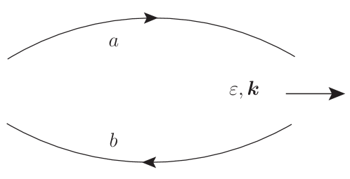
(a) Particle-hole pair

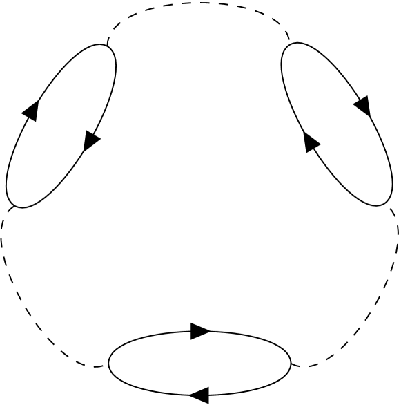
(b) Ring diagram

(c) Ladder diagram

Figure 1: Figure (a) represents the particle-hole bubble $\Pi_{ab}(\varepsilon,\bm{k})$. Note that the spins $a$ and $b$ can be different. (b) and (c) are examples of ring and ladder diagrams respectively, each showing three particle-hole pairs joined together.

These pair fluctuation are bosonic and remain soft down to zero momentum. The long-ranged correlation of these bosonic modes is not strong enough to cause full-fledged infrared divergence in the present case, but results in weaker logarithmic corrections only at higher orders. This is the origin of the non-analyticity. For a review of this “soft mode” paradigm, and in particular how it affects the critical behavior, see Belitz and Vojta (2005) and the references therein.

These soft modes must be cut off by some relevant infrared scale. Temperature is an obvious candidate. In the presence of $(H_{a}-H_{b})\neq 0$, it can be seen that the energy of pair excitation $\Pi_{ab}$ is shifted by $(H_{a}-H_{b})$; therefore the magnetic field can also serve as the cutoff. One expects the larger of the two scales to dominate, and this hints at possible crossover behavior when the ratio $T/H$ is varied continuously between the two extremes Betouras et al. (2005). However, each particle-hole pair in the ring diagram is of the same spin, and is insensitive to the magnetic field. The crossover behavior is thus exhibited only in the ladder-type non-analyticity.

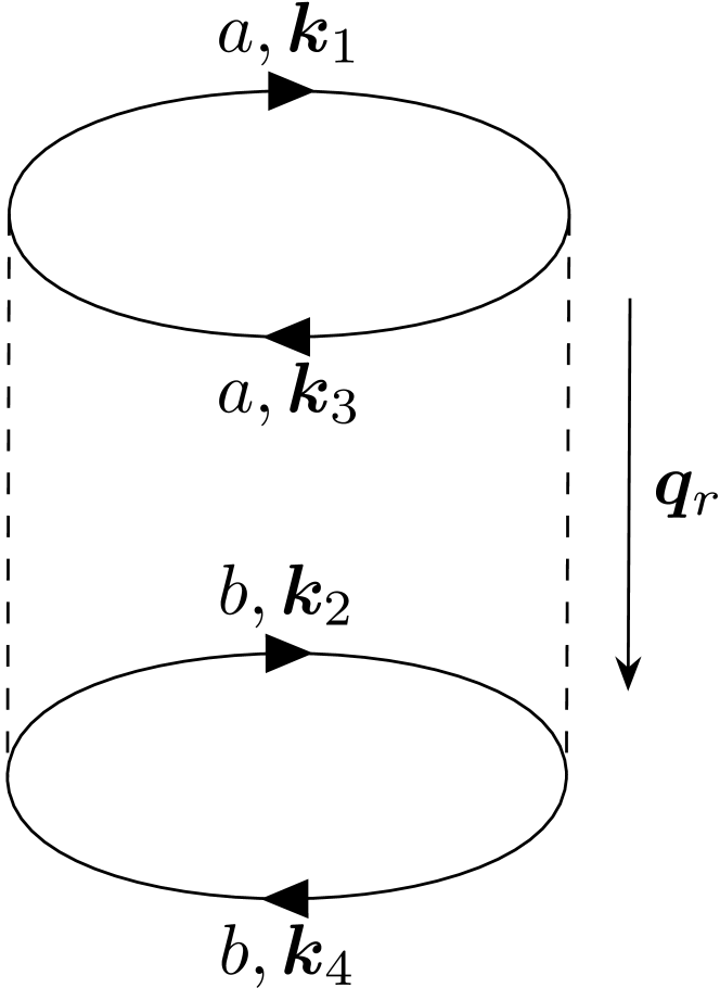
(a) Ring diagram

(b) Ladder diagram

Figure 2: The ring and ladder forms of the same second-order vacuum Feynman diagram. The small-momentum limits of the forms corresponds to the limit where $\bm{q}_{r}=\bm{k}_{1}-\bm{k}_{3}$ or $\bm{q}_{l}=\bm{k}_{1}-\bm{k}_{4}$ vanishes, respectively. This term is labeled as $\Omega_{2a}$.

In this paper we work to second order in perturbation theory. The ring and ladder diagram at second order is actually one and the same, as shown in figure 2. However, the two small-momentum limits refer to distinct regions of the momentum integral.

At second order, the ring diagram is known to yield further non-analytic terms in the region $q_{r}\approx 2k_{F}$ Chubukov et al. (2006). Historically this has been linked to the dynamic Kohn anomaly Amit et al. (1968a); Pethick and Carneiro (1973); Chubukov et al. (2006). However, this non-analytic contribution only comes from the limit where $\bm{q}_{1}$ and $\bm{q}_{2}$ are anti-parallel Amit et al. (1968a), and can be identified with the small-$q_{l}$ limit of the ladder diagram Chubukov et al. (2006); Maslov and Chubukov (2009). Conversely, the ladder diagram also contributes to the non-analyticity around $q_{l}\approx 2k_{F}$, and this translates to the small-$q_{r}$ limit of the ring diagram.

We argue that, rather than the traditional “zero-and-$2k_{F}$” picture, it is more natural to look at the non-analyticity as coming solely from the zero-momentum limit of particle-hole pairs, but then consider all possible spin combinations.

II.3 Possible Form of $\Omega$

The thermodynamic potential is $\Omega=-T\ln Z$. In the thermodynamic limit, it is more convenient to consider the intensive quantity $\Omega/V$, where $V$ is the volume of space.

The usual GL paradigm dictates that $\Omega$ be an analytic function of $T$ and $H$. Coupled with the symmetry of the problem, one expects that $\Omega$ can be expanded as a polynomial of $T^{2}$ and $H^{2}$ only. But the known $T^{3}\ln T$ specific heat and $H^{2}\ln H$ spin susceptibility implies that the GL picture is no good already at fourth order.

Define the dimensionless quantities $t=T/\mu_{0}$ and $h=H/\mu_{0}$. On dimensional ground, and with the knowledge that the Sommerfeld expansion cannot generate odd powers of $T$, one writes down schematically the possible form of $\Omega$, omitting all coefficients:

$$\frac{\Omega}{V}\sim v_{\mu}k_{\mu}^{4}\left\{1+\left(t^{2}+h^{2}\right)+F_{4}(t,h)+\dots\right\}.$$ (4)

Here the (generalized) fourth order term $F_{4}$ is defined to be the sum of all terms that scale as $(\text{energy})^{4}$, up to possible logarithmic dependence. We know that $F_{4}$ must be non-analytic at $T=H=0$. Its behavior near the origin of the $(T,H)$-plane will depend on the direction of approach. In particular, if one attempts a double expansion of $F_{4}$ in $t$ and $h$, the result will depend on the order in which the expansions are carried out.

II.4 What Is Fermi Liquid and What Is Not?

First verified by Pethick and CarneiroPethick and Carneiro (1973), an oft-repeated observation is that the leading logarithmic correction is a “universal” feature of any FL. This raises the question: in the expression (4), what can be considered “universal”?

We try to address this question in the context of a dilute Fermi gas. FL is then a low-energy effective theory of the model, with only degrees of freedom near the Fermi surface. One can take a linearized quasiparticle dispersion and an approximated constant density of state around the Fermi surface as the working definition of this effective theory. All the higher-energy modes are integrated out, renormalizing the parameters of this effective theory.

Furthermore, FL is only accurate when all external scales in the problem, such as $T$ and $H_{a}$, are dwarfed by the Fermi sea. In other words, $\mu_{0}$ and $k_{F}$ should be considered essentially infinite when compared with other scales. This means that, at high enough order, terms in (4) will eventually be deemed infinitesimal and outside the scope of FL.

For the non-interacting gas, one can calculate $\Omega$ exactly. It can be shown that the leading correction to the free gas (second order in $t$ and $h$) in (4) depends only on Fermi velocity and density of state at Fermi surface . So one can conclude that these are within the FL picture, while fourth and higher order terms are beyond FL. In contrast, the non-analytic terms at fourth order do come from the Fermi surface only, as mentioned above.

To go beyond dilute limit and perturbation theory, one can replace Fermi velocity, density of state, and scattering amplitudes of quasiparticles with their fully renormalized values, as suggested in refs Chubukov et al. (2006); Maslov and Chubukov (2009). By construction, this simple replacement yields FL results (second and third order terms, and the fourth order logarithmic correction) that remain valid in the strongly-interacting regime. This however will not apply to terms outside the scope of FL, and we lose all ability to calculate them in the strongly interacting regime.

III Sommerfeld Expansion of $\Omega$ for Fermi Gas

In this section, we take a break from the FL picture, and attempt to evaluate the thermodynamic potential of a weakly interacting Fermi gas. This will confirm some assertions made in section II.2, and also give us some hints on the possible form of $F_{4}$.

(a) $\Omega_{1}$

(b) $\Omega_{2b}$

Figure 3: The Hartree-Fock diagrams contributing to the thermodynamic potential $\Omega$ to second order.

We wish to calculate the thermodynamic potential of the gas. To second order of perturbation theory, there are three Feynman diagrams to be included. Following the notation of the prequel Cheng and Yip (2017), we label these three terms as $\Omega_{1}$, $\Omega_{2a}$ and $\Omega_{2b}$, respectively. Depicted in Figure 3, $\Omega_{1}$ and $\Omega_{2b}$ are part of the Hartree-Fock approximation and are analytic in $T$ and $H$. On the other hand, $\Omega_{2a}$ as shown in Figure 2 is both a ring and a ladder diagram, and is solely responsible to non-analyticity of $\Omega$ at this level of approximation.

In this section, we will first attempt an expansion in $T$, writing $\Omega=\alpha_{0}(H)+\alpha_{2}(H)\,t^{2}+\dots$ at finite $H$. Analytic closed form solutions of these $H$-dependent coefficients can be obtained, but we found that it is much more elucidating to further expand each coefficient in series of $H$. Please see appendix A for more detail.

To maintain consistency with the prequel, we define the dimensionless lowercase $\omega$’s via

$$\begin{split}\frac{\Omega}{V}=\frac{k_{\mu}^{3}}{6\pi^{2}}\frac{k_{\mu}^{2}}{2m}\sum_{a=1}^{\mathcal{N}_{c}}\Bigg{[}\omega_{0}^{(a)}+(k_{\mu}a)\sum_{b\neq a}\omega_{1}^{(ab)}\\ +(k_{\mu}a)^{2}\left(\sum_{b\neq a}\omega_{2a}^{(ab)}+\sum_{b\neq a}\sum_{c\neq a}\omega_{2b}^{(abc)}\right)+\dots\Bigg{]}.\end{split}$$ (5)

where each $\omega_{x}$ originates from the respective $\Omega_{x}$ with the same label. We have temporarily restored $\mathcal{N}_{c}$ in the above expression. For $\mathcal{N}_{c}=2$, the sum over spin is quite trivial and we define the spin-symmetrized version:

$$w_{0}= \;\frac{1}{2}\left(\omega_{0}^{(\uparrow)}+\omega_{0}^{(\downarrow)}\right);$$ (6a)

$$w_{1}= \;\frac{1}{2}\left(\omega_{1}^{(\uparrow\downarrow)}+\omega_{1}^{(\downarrow\uparrow)}\right);$$ (6b)

$$w_{2a}= \;\frac{1}{2}\left(\omega_{2a}^{(\uparrow\downarrow)}+\omega_{2a}^{(\downarrow\uparrow)}\right);$$ (6c)

$$w_{2b}= \;\frac{1}{2}\left(\omega_{2b}^{(\uparrow\downarrow\uparrow)}+\omega_{2b}^{(\downarrow\uparrow\downarrow)}\right).$$ (6d)

III.1 Free Gas and Hartree-Fock Contributions

Let $\epsilon(k)$ denotes the kinetic energy of free gas, $n_{a}(x)$ the Fermi function for fermions with spin $a$, and $N_{a}^{0}$ the non-interacting number density for these fermions:

$$\epsilon(k)\equiv \;\frac{k^{2}}{2m};$$ (7a)

$$n_{a}(k)\equiv \;\left(e^{\beta(\epsilon(k)-\mu_{a})}+1\right)^{-1};$$ (7b)

$$N_{a}^{0}\equiv \int\!\!\frac{\mathrm{d}^{3}k}{(2\pi)^{3}}\,n_{a}\!(k).$$ (7c)

The thermodynamic potential of a free gas is given by

$$\frac{\Omega_{0}}{V}=T\sum_{a=\uparrow,\downarrow}\int\!\!\frac{\mathrm{d}^{3}k}{(2\pi)^{3}}\,\ln\!\left(1-n_{a}\!\left(k\right)\right).$$ (8)

Likewise, the two Hartree-Fock terms $\Omega_{1}$ and $\Omega_{2b}$ are:

$$\frac{\Omega_{1}}{V}= \left(\frac{4\pi a}{m}\right)N_{\uparrow}^{0}N_{\downarrow}^{0};$$ (9)

$$\frac{\Omega_{2b}}{V}= \left(\frac{4\pi a}{m}\right)^{\!2}\frac{1}{2}\left[\left(\frac{\partial N_{\uparrow}^{0}}{\partial\mu_{0}}\right)N_{\downarrow}^{0}N_{\downarrow}^{0}+\left(\frac{\partial N_{\downarrow}^{0}}{\partial\mu_{0}}\right)N_{\uparrow}^{0}N_{\uparrow}^{0}\right].$$ (10)

From here one can identify the associated dimensionless $\omega_{0}$, $\omega_{1}$ and $\omega_{2b}$. Up to fourth order in $t$ and $h$, they are

$$w_{0}=\; -\frac{2}{5}-\frac{\pi^{2}}{4}t^{2}-\frac{1}{16}h^{2}+\frac{7\pi^{4}}{960}t^{4}+\frac{1}{1024}h^{4}+\frac{\pi^{2}}{128}t^{2}h^{2};$$ (11a)

$$w_{1}=\; \frac{2}{3\pi}+\frac{\pi}{6}t^{2}-\frac{1}{4\pi}h^{2}+\frac{\pi^{3}}{40}t^{4}+\frac{1}{64\pi}h^{4}+\frac{\pi}{16}t^{2}h^{2};$$ (11b)

$$w_{2b}=\; -\frac{4}{3\pi^{2}}-\frac{5}{18}t^{2}-\frac{11}{24\pi^{2}}h^{2}-\frac{17\pi^{2}}{1440}t^{4}+\frac{47}{512\pi^{2}}h^{4}+\frac{35}{192}t^{2}h^{2}.$$ (11c)

III.2 The Two-Bubble Diagram $\Omega_{2a}$

The term $\Omega_{2a}$ (Figure 2) is unique among all vacuum diagrams: depending on how the diagram is arranged, the scattering process involved can be seen as taking place in any one of the three channels: scattering of a particle-hole pair of the same spin, scattering of a particle-hole pair of different spins, and scattering of a particle-particle pair. The first two corresponds to the “ring” and “ladder” classifications, respectively. The particle-particle Cooper channel is linearly divergent in the UV, and we implicitly subtract off the diverging part. In the remainder of this section, we will consider the diagram exclusively in the ring configuration. Setting $\mathcal{N}_{c}=2$, the Feynman diagram in Figure 2(a) yields:

$$\frac{\Omega_{2a}}{V}=-\left(\frac{4\pi a}{m}\right)^{\!2}\!\!\int\prod_{i=1}^{3}\frac{\mathrm{d}^{3}\bm{k}_{i}}{(2\pi)^{3}}\frac{n_{\uparrow}(k_{1})n_{\downarrow}(k_{2})\left[n_{\uparrow}(k_{3})+n_{\downarrow}(k_{4})\right]}{\frac{1}{2m}\left[k_{1}^{2}+k_{2}^{2}-k_{3}^{2}-k_{4}^{2}\right]},$$ (12)

where $\bm{k}_{1}+\bm{k}_{2}-\bm{k}_{3}-\bm{k}_{4}=0$ by momentum conservation.

From here one identifies the quantity $w_{2a}$ as defined in (6):

$$w_{2a}(t,h)=\frac{6\pi^{2}m}{k_{\mu}^{7}a^{2}}\frac{\Omega_{2a}(T,H)}{V}.$$ (13)

In the prequel, this term was examined numerically at $H=0$. It has the form:

$$w_{2a}(t,0)=B+C_{1}\,t^{2}+D_{1}\,t^{4}\ln t+E_{1}\,t^{4}+\dots$$ (14)

On the other hand, at zero temperature the integral (12) can be done analytically Kanno (1970), yielding

$$w_{2a}(0,h)=B+C_{2}\,h^{2}+D_{2}\,h^{4}\ln|h|+E_{2}\,h^{4}+\dots$$ (15)

Next, we attempt the double expansion, first in $t$ and then in $h$. The result is of the form:

$$w_{2a}(t,h)=B+C_{1}\,t^{2}+C_{2}\,h^{2}+f_{4}(t,h)+(\text{sixth order}),$$ (16)

where the fourth order term $f_{4}$ is

$$\begin{split}f_{4}(t,h)=&\;\frac{1}{2}D_{1}\,t^{4}\left(\ln|h|+\ln\Delta\right)+D_{2}\,h^{4}\ln|h|\\ &+F_{1}\,t^{4}+E_{2}\,h^{4}+F_{3}\,t^{2}h^{2}\\ &+t^{4}\left[\xi\!\left(t,\Delta\right)+\sum_{i=1}^{\infty}F_{4,i}\left(\frac{t}{h}\right)^{2i}\right].\end{split}$$ (17)

Here $\Delta$ is an infinitesimal infrared cutoff imposed on the momentum transfer $\bm{q}_{r}=\bm{k}_{1}-\bm{k}_{3}$ to regularize the results. (See the appendix A for the complication of a momentum cutoff.)

Apart from the infinitely many $F_{4,i}$, all coefficients appearing in (14), (15) and (17) are given in table 1.

$B$	$\displaystyle\frac{4(11-2\ln 2)}{35\pi^{2}}$
$C_{1}$	$\displaystyle-\ln 2+\frac{1}{2}$
$C_{2}$	$\displaystyle-\frac{(1+2\ln 2)}{8\pi^{2}}$
$D_{1}$	$\displaystyle-\frac{\pi^{2}}{10}$
$D_{2}$	$\displaystyle\frac{1}{32\pi^{2}}$
$E_{1}$	$1.62$
$E_{2}$	$\displaystyle\frac{29-102\ln 2}{1536\pi^{2}}$
$F_{1}$	$\displaystyle\frac{6597-704\ln 2}{38400\pi^{2}}$
$F_{3}$	$\displaystyle\frac{19-6\ln 2}{64}$
$\kappa$	$1.70$

Table 1: The coefficients for of $w_{2a}$. The value of $E_{1}$ comes from the numerical fit in the prequel Cheng and Yip (2017). The value of $\kappa$ is determined by equation (29).

Instead of a non-analytic $t^{4}\ln t$ term, we found $t^{4}\left(\ln h+\ln\Delta\right)$. Going to higher orders in $T$, we found increasingly singular terms with powers of $h$ and $\Delta$ in the denominator, combining to an overall fourth order. We are naturally unable to carry this calculation to infinite order in $T$, but it is not difficult to infer, using dimensional analysis and symmetry argument, that the $h$ part forms an infinite series of $(t/h)^{2n}$.

In (17), we denote the $\Delta$ counterpart of these higher singular terms as $\xi(t,\Delta)$. We made no attempt to infer a general form of $\xi$. But it is clear that the original integral (12) is finite. One therefore concludes that all infrared divergent terms must resum into a finite quantity; that is,

$$\frac{1}{2}D_{1}\ln\Delta+\xi(t,\Delta)=\frac{1}{2}D_{1}\ln t+\kappa,$$ (18)

where $\kappa$ is a constant yet unknown. It will be determined later by matching with the numerical result (14).

Note that when one sets $t$ to zero, $f_{4}(0,h)$ as given in (17) reduces to $D_{2}h^{4}\ln h+E_{2}h^{4}$, in exact agreement with (15).

By imposing an upper cutoff in $|\bm{q}_{r}|$ that is smaller than the Fermi momentum, we also verified that the $t^{4}\ln h$ term has contribution only from $2\sqrt{2m\mu_{\downarrow}}<|q_{r}|<2\sqrt{2m\mu_{\uparrow}}$. That is, it comes from the region where $|q_{r}|\approx 2k_{F}$, confirming the earlier claim in the literature Chubukov et al. (2006); Maslov and Chubukov (2009).

The absence of a logarithmic term with the $t^{2}h^{2}$ prefactor in (17) is notable. The accepted wisdom Carneiro and Pethick (1977) is such that the spin susceptibility does not scale as $T^{2}\ln T$, which is in line with our result here. Granted, in the present form (17) is only appropriate when $t/h\ll 1$, while spin susceptibility is defined near zero magnetic field. But the coefficients to the logarithmic terms are robust: resummation of the series $(t/h)^{2i}$ cannot generate a separate $t^{2}h^{2}$ logarithmic term. If it is absent for $t/h\ll 1$, it must remain so for all values of the ratio.

IV Resumming the Singular Terms: Fermi Liquid Picture

The original loop integral (12) is finite when $h$ is set to zero. Yet the expression (17) is not even well-defined in the same limit.

To obtain a well-defined expression for $f_{4}$ in this limit, in principle one only needs to swap the order of $h$- and $t$-expansion. Unfortunately, we cannot analytically evaluate the resultant integrals. Instead, we will identify the $2k_{F}$ non-analyticity of (12) with the infrared non-analyticity of the ladder diagram (figure 2(b)), and evaluate the latter exactly within the FL picture.

IV.1 The equivalence between Ladder and $2k_{F}$ Non-analyticity

Historically, the study of non-analyticity of FL was framed in terms of the quasiparticle self-energy. Amit, Kane and Wagner Amit et al. (1968a) were the first to observe that interaction with a particle-hole pair at either zero or $2k_{F}$ momentum results in the leading logarithmic correction to the self-energy. In a lengthy paper, Chubokov and Maslov Chubukov and Maslov (2003) established that the non-analytic contribution from the scattering of a particle-hole pair at $2k_{F}$ is exactly equivalent to that of a particle-particle pair at zero momentum. Noting that the proper self-energy is obtained by differentiating vacuum 2PI Feynman diagrams, the above result essentially constitutes a proof that, for our $\Omega_{2a}$ term (see figure 2), the $|q_{l}|=0$ non-analyticity is equivalent to that of $|q_{r}|\rightarrow 2k_{\mu}$. Nevertheless we will offer a standalone argument here, applied specifically to $\Omega_{2a}$.

Non-analyticity of $\Omega_{2a}$ must come from where the integrand in (12) is singular at $T=H=0$. One notes that the denominator of the integrand is proportional to $(\bm{q}_{l}\cdot\bm{q}_{r})$. It may then appear that there are three separate cases: $\bm{q}_{l}=0$, $\bm{q}_{r}=0$, and $\bm{q}_{l}\perp\bm{q}_{r}$. However, one can find a suitable change of variables such that the integration measure transforms as

$$\mathrm{d}^{3}\bm{k}_{1}\,\mathrm{d}^{3}\bm{k}_{2}\,\mathrm{d}^{3}\bm{k}_{3}\rightarrow\mathrm{d}^{3}\bm{q}_{r}\,\mathrm{d}^{3}\bm{q}_{l}\,\mathrm{d}^{3}\!\bm{X},$$ (19)

where $\bm{X}$ is some way to represent the remaining three degrees of freedom. It is clear that the vanishing integration measure renders the limits $\bm{q}_{l}\rightarrow 0$ and $\bm{q}_{r}\rightarrow 0$ regular by themselves. The only actual singularity is where $\bm{q}_{l}$ and $\bm{q}_{r}$ are orthogonal to each other.

We have shown at the end of section III.2 that the non-analytic terms come from either $|\bm{q}_{r}|\rightarrow 0$ or $|\bm{q}_{r}|\rightarrow 2k_{\mu}$, and let us concentrate on the $2k_{\mu}$ condition. The region of the momentum integration that contributes to the non-analyticity must then satisfy both the $2k_{\mu}$ and the orthogonality conditions.

Let us now analyze the part of (12) that is proportional to $n_{\uparrow}(k_{1})\,n_{\downarrow}(k_{2})\,n_{\uparrow}(k_{3})$. At zero temperature and magnetic field, these Fermi functions all become the step function, restricting $\bm{k}_{1}$, $\bm{k}_{2}$ and $\bm{k}_{3}$ to within the Fermi sphere. The $2k_{\mu}$ condition forces $\bm{k}_{1}$ and $\bm{k}_{3}$ to sit exactly on the Fermi surface, and be polar opposite to one another. Note that by momentum conservation $\bm{q}_{l}=\bm{k}_{3}-\bm{k}_{2}$. The orthogonality condition then forces $\bm{q}_{l}$ to vanish. See Fig 4 for illustration.

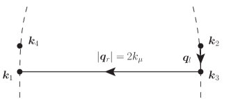
Figure 4: The configuration around which the $2k_{\mu}$ non-analyticity of $\Omega_{2a}$ comes from. The dashed lines represent the Fermi sphere. The requirements are $|\bm{q}_{r}|\rightarrow 2k_{\mu}$, $\bm{q}_{l}\perp\bm{q}_{r}$, and that $\bm{k}_{1},\ldots\bm{k}_{3}$ lie within the Fermi sphere. Consequently $\bm{q}_{l}$ must vanish, and all four momenta $\bm{k}_{1},\ldots\bm{k}_{4}$ must be exactly on the Fermi surface.

For the other part of (12) where $n_{\uparrow}(k_{3})$ is replaced by $n_{\downarrow}(k_{4})$, one can identify $\bm{q}_{r}=\bm{k}_{2}-\bm{k}_{4}$ and $\bm{q}_{l}=\bm{k}_{1}-\bm{k}_{4}$, and the same argument goes through.

One can reverse the argument to show that the $\bm{q}_{l}\rightarrow 2k_{\mu}$ non-analyticity is always paired with the limit $\bm{q}_{r}\rightarrow 0$. It is thus concluded that non-analyticity of $\Omega_{2a}$ comes from the limiting regions of momentum integration where one of $\bm{q}_{r}$ and $\bm{q}_{l}$ vanishes, and the other approaches $2k_{\mu}$.

This can be thought of as a duality between the ring and ladder diagrams (see Fig. 2): the $2k_{\mu}$ non-analyticity in the ring form is exactly the zero-momentum non-analyticity in the ladder form, and vice versa.

Finally we note that, in either limit, $\bm{k}_{4}$ is forced to sit on the Fermi surface too by momentum conservation. Therefore, to capture the non-analyticity of $\Omega_{2a}$, it suffices to consider the small-momentum limit of both ring and ladder diagrams in Fig 2, with all four fermion legs restricted to be near the Fermi surface.

IV.2 Ladder Diagram and Fermi Liquid Approximation

Consider the ladder Feynman diagram (Fig 2(b)), which gives the term $\Omega_{2a}^{ab}$ before summing over spins. The Feynman diagram can be understood as the trace of the square of particle-hole Green’s function $\Pi_{ab}(i\nu,q)$, where $\nu$ is the Bosonic Matsubara frequency. This reduces to equation (12) if the full non-interacting form of $\Pi_{\uparrow\!\downarrow}$ is used.

However, our present goal is to compute all non-analytic terms not coming from $|q_{r}|\rightarrow 0$, and the preceding discussion made clear that one only needs to look at a limit: $|\bm{q}_{l}|\rightarrow 0$, with $\bm{k}_{1},\ldots\bm{k}_{4}$ all near the Fermi surface. One can then employ the asymptotic form of $\Pi_{\uparrow\!\downarrow}$ for small $q$, denoted $\pi_{\uparrow\!\downarrow}$:

$$\pi_{\uparrow\!\downarrow}(\varepsilon,q)=\frac{k_{\mu}^{2}}{(2\pi)^{2}v_{\mu}}\left\{2+\frac{\varepsilon}{v_{\mu}\,q}\ln\left[\frac{\left(\frac{\varepsilon+H}{v_{\mu}\,q}\right)-1}{\left(\frac{\varepsilon+H}{v_{\mu}\,q}\right)+1}\right]\right\}.$$ (20)

Corrections to this approximated form come in as positive powers of $(H/v_{\mu}\,k_{\mu})^{2}$, $(T/v_{\mu}\,k_{\mu})^{2}$, or $(q/k_{\mu})^{2}$. Since $k_{\mu}$ is to be viewed as an ultraviolet scale of the FL effective theory, these corrections are to be regarded as vanishingly small in the present approximation. It is also not difficult to see that these beyond-FL corrections only yield overall sixth order terms and higher if they are included in the following calculation.

We define a modified $\tilde{w}_{2a}$ based on $w_{2a}$, with the full particle-hole bubble $\Pi_{\uparrow\!\downarrow}$ replaced by $\pi_{\uparrow\!\downarrow}$:

$$\tilde{w}_{2a}(t,h)=-\left(\frac{24\pi^{4}}{k_{\mu}^{7}m}\right)\,T\sum_{\nu}\int^{\Lambda}\!\!\frac{\mathrm{d}^{3}q}{(2\pi)^{3}}\;\left(\pi_{\uparrow\!\downarrow}(i\nu,q)^{2}+\pi_{\downarrow\!\uparrow}(i\nu,q)^{2}\right).$$ (21)

This quantity contains the contribution to $w_{2a}$ coming from the $q_{l}\rightarrow 0$ region of the momentum integral. Due to the small-$q$ approximation, a large-momentum cutoff $\Lambda$ is necessary to render the expression finite. We assume the hierarchy of scales: $v_{\mu}k_{\mu}\gg v_{\mu}\Lambda\gg T,H$.

With a convergence factor $e^{i\omega o^{+}}$ appended, the Matsubara frequency sum in (21) can be carried out using standard contour integration tricks. The sum is transformed into an integral over energy $\varepsilon$, weighted by the usual Bose function $n_{B}(\varepsilon)=(e^{\beta\varepsilon}-1)^{-1}$, around the branch cut of $\pi_{ab}(\varepsilon,q)^{2}$ on the real axis. The energy integral only picks up the discontinuity of the integrand across the branch cut, which is precisely the imaginary part. The integration in $\bm{q}$ can also be carried out.

The end result contains a number of analytic terms: $T^{4}$, $H^{4}$, $T^{2}H^{2}$, $\Lambda^{2}T^{2}$, $\Lambda^{2}H^{2}$, and $\Lambda^{4}$. The cutoff $\Lambda$ appears here because the omitted large-$q$ processes can nonetheless have small energy, and contribute equally well at order $T^{2}$ and $H^{2}$. The cutoff dependence signals the incompleteness of our treatment. This nevertheless poses no problem, as we only want to capture the non-analytic terms with this approach. The non-analytic part of (21) reads:

$$\begin{split}\tilde{w}_{2a}(t,h)=-\frac{3m^{4}}{\pi^{2}k_{\mu}^{8}}\left\{\,2\!\int_{0}^{\infty}\!\!\mathrm{d}\varepsilon\;n_{B}(\varepsilon)\,\varepsilon^{2}(\varepsilon+H)\ln\left|\frac{\varepsilon+H}{v_{\mu}\Lambda}\right|+\int_{0}^{v_{F}\Lambda-H}\!\!\mathrm{d}\varepsilon\;\varepsilon^{2}(\varepsilon+H)\ln\left|\frac{\varepsilon+H}{v_{\mu}\Lambda}\right|\right\}\\ +(H\rightarrow-H)+(\text{analytic}).\end{split}$$ (22)

The second term above can be integrated to yield $h^{4}\ln|H/v_{\mu}\Lambda|$ plus analytic terms. In addition, one can split $\ln|(\varepsilon+H)/v_{\mu}\Lambda|=\ln|\varepsilon/v_{\mu}\Lambda|+\ln|(\varepsilon+H)/\varepsilon|$ in the integrand and notes that

$$\frac{1}{2}\,D_{1}t^{4}\ln\left(\frac{T}{v_{\mu}\Lambda}\right)=-\frac{6m^{4}}{\pi^{2}k_{\mu}^{8}}\int_{0}^{\infty}\!\!\mathrm{d}\varepsilon\;n_{B}(\varepsilon)\,\varepsilon^{3}\ln\left|\frac{\varepsilon}{v_{\mu}\Lambda}\right|+(\text{analytic}).$$ (23)

This relation can be used to write $\tilde{w}_{2a}$ in the following form:

$$\tilde{w}_{2a}(t,h)=\chi(t,h)+\frac{1}{2}D_{1}\,t^{4}\ln t+D_{2}\,h^{4}\ln h+(\text{analytic}),$$ (24)

where the crossover function $\chi(t,h)$ is defined as

$$\chi(t,h)=-\frac{6m^{4}}{\pi^{2}k_{\mu}^{8}}\int_{0}^{\infty}\!\!\mathrm{d}\varepsilon\;n_{B}(\varepsilon)\,\varepsilon^{2}\left[(\varepsilon+H)\ln\left|\frac{\varepsilon+H}{\varepsilon}\right|+(\varepsilon-H)\ln\left|\frac{\varepsilon-H}{\varepsilon}\right|\right].$$ (25)

The expression (24) and (25) capture all the ladder-type non-analytic terms, which we were unable to obtain to infinite order using the Sommerfeld expansion approach in (17). Indeed, both $t^{4}\ln t$ and $h^{4}\ln|h|$ are recovered with correct coefficients.

In order to make comparison with (16) and (17), one needs to evaluate $\chi(t,h)$ in the limit where the ratio $\alpha=t/h\ll 1$. This is accomplished by expanding out the logarithm in (25), assuming $\varepsilon/H$ is always small. The expansion is justified because the Bose function $n_{B}(\varepsilon)$ allows only contribution from the range $\varepsilon<T$. The result is:

$$\begin{split}\chi(t,h)=&\;\frac{1}{2}D_{1}\,t^{4}\ln\left(\frac{h}{t}\right)\\ &+t^{4}\left[\frac{\pi^{4}(5-6\gamma_{E})+540\,\zeta^{\prime}(4)}{120\pi^{2}}+\mathcal{O}\!\left(\alpha^{2}\right)\right].\end{split}$$ (26)

One immediately notes that the $\ln|h/t|$ term correctly converts the $\ln t$ in (24) into $\ln|h|$ in the limit $\alpha\rightarrow 0$ where $h$ dominates over $t$.

Finally one can compare (24) and (26) with (16) and (17), and identify the $\mathcal{O}\!\left(\alpha^{2}\right)$ terms in (26) with the infinite series in (17). This yields:

$$\begin{split}\sum_{i=1}^{\infty}F_{4,i}\alpha^{2i}=&\;\frac{\chi(t,h)}{t^{4}}+\frac{1}{2}D_{1}\ln\left(\alpha\right)\\ &-\left(\frac{\pi^{4}(5-6\gamma_{E})+540\,\zeta^{\prime}(4)}{120\pi^{2}}\right).\end{split}$$ (27)

As an extra check, we computed the coefficient $F_{4,1}$ both using Sommerfeld expansion and from the crossover function $\chi(t,h)$. Both approaches give identical answer $F_{4,1}=\pi^{4}/63$.

IV.3 $\Omega_{2a}$ Near The $T$-axis

The infinite series in (17) has been resummed using (27). It is natural to ask if one can now find a well-defined expression for $w(t,h)$ when the ratio $\alpha$ is large.

As it turns out, it is quite tricky to expand $\chi(t,h)$ around a small $1/\alpha$. We relegate the detail to the appendix, and note the result here:

$$\begin{split}\chi(t,h)=&\,D_{2}\,h^{4}\ln\!\left(\frac{t}{h}\right)-\frac{1}{16}t^{2}h^{2}\\ &+h^{4}\left[\frac{12(\ln 2\pi-\gamma_{E})+7}{384\pi^{2}}+\mathcal{O}\!\left(\!\frac{1}{\alpha^{2}}\!\right)\right].\end{split}$$ (28)

Equations (27) and (28) can be substituted into (17) to give an expression of $f_{4}(t,h)$ well-defined in the limit of large $\alpha$. In particular, we are finally in a position to determine the constant $\kappa$ appearing in (18). Matching the coefficient of $t^{4}$ terms, one obtains:

$$E_{1}=F_{1}-\left(\frac{\pi^{4}(5-6\gamma_{E})+540\,\zeta^{\prime}(4)}{120\pi^{2}}\right)+\kappa,$$ (29)

which yields $\kappa=1.51$.

With this final piece of puzzle found, one has the complete non-analytic equation of state of a dilute Fermi gas up to overall fourth order in $t$ and $h$. The fourth order term $f_{4}(t,h)$ as defined in (16) is non-analytic, and its series expansion takes different forms depending on the size of $\alpha=t/h$.

When $\alpha\lesssim 1$, one has

$$\begin{split}f_{4}(t,h)=&\;\frac{D_{1}}{2}\,t^{4}(\ln h+\ln t)+D_{2}\,h^{4}\ln h\\ &+(F_{1}+\kappa)t^{4}+E_{2}h^{4}+F_{3}t^{2}h^{2}\\ &+t^{4}\sum_{i=1}^{\infty}\left(F_{4,i}\,\alpha^{2i}\right).\end{split}$$ (30)

The coefficients $F_{4,i}$ for arbitrary $i$ can be computed using (27). Or even better, one can just numerically evaluate $\chi(t,h)$ to resum the series.

One can obtain the corresponding expansion for $\alpha\gtrsim 1$ using (28). The result is

$$\begin{split}f_{4}(t,h)=&\;D_{1}\,t^{4}\ln t+D_{2}\,h^{4}\ln t\\ &+E_{1}t^{4}+G_{2}h^{4}+G_{3}t^{2}h^{2}\\ &+h^{4}\sum_{i=1}^{\infty}\left(G_{4,i}\,\alpha^{-2i}\right),\end{split}$$ (31)

with $G_{2}=E_{2}+\frac{12(\ln 2\pi-\gamma_{E})+7}{384\pi^{2}}$ and $G_{3}=F_{3}-\frac{1}{16}$. The infinite series in (31) sums to:

$$\begin{split}\sum_{i=1}^{\infty}G_{4,i}\,\alpha^{-2i}=&\;\frac{\chi(t,h)}{h^{4}}-D_{2}\,\ln\!\left(\alpha\right)+\frac{1}{16}\alpha^{2}\\ &-\left[\frac{12(\ln 2\pi-\gamma_{E})+7}{384\pi^{2}}\right].\end{split}$$ (32)

V The Crossover Behavior

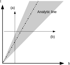
Figure 5: This is a sketch of the crossover behavior of the ladder-type non-analyticity. The shaded crossover region separates the two near-axis areas, where one scale dominates the other. The analytic line in the crossover region is where the two sets of non-analyticity precisely cancel each other out. The two paths (a) and (b) will be considered in subsequent discussion.

As discussed in section II.2, the ladder-type non-analyticity (figure 2(b)) can be cut off in the infrared by either $T$ or $H$. The competition between the two scales results in a non-trivial crossover. We sketch the behavior in figure 5.

Consider the expression (16) for $w$. The non-analytic $f_{4}$ term admits two different expansions (30) and (31), good for the regions near the $t$- and $h$-axis in figure 5, respectively. When the ratio $\alpha=t/h$ is neither larger nor small, the higher order terms are important in both expansions, and this corresponds to the shaded crossover region. Fortunately, the series can be resum exactly using (27) and (32).

V.1 Path (a): Raising $t$ with a fixed $h$

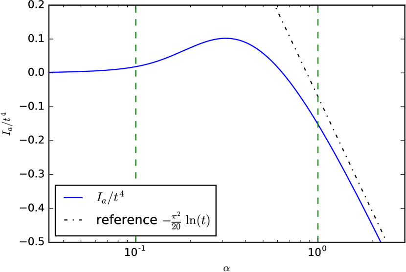
(a)

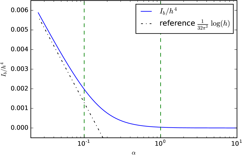
(b)

Figure 6: The plots of the ladder-type non-analytic parts (a) $I_{a}/t^{4}$ and (b) $I_{b}/h^{4}$ against $\ln\alpha$. (a) is up to a vertical offset of $\ln h$, while (b) is up to a vertical offset of $\ln t$. The green dashed lines indicate the crossover regions on each plot, corresponding to the shaded area in FIG 5. Each curve approaches zero on one side of the crossover region, indicating the asymptotic $t^{4}\ln h$ and $h^{4}\ln t$ behaviors of $I_{a}$ and $I_{b}$, respectively. On the opposite sides of the crossover region, $I_{a}$ and $I_{b}$ respectively become $t^{4}\ln t$ and $h^{4}\ln h$, as indicated by the asymptotically linear behavior.

This is perhaps the scenario most relevant to the experiment. As the effective magnetic field is controlled via the number densities of individual spin components, moving along path (a) in figure 5 corresponds to fixing the composition of the gas and tuning the temperature.

In region near the $h$-axis, (30) is the appropriate expression to use. To identify the ladder-type non-analyticity, from the thermodynamic potential one subtracts off all the analytic terms, and half of the total $t^{4}\ln t$ term associated with the ring-type non-analyticity. The result reads:

$$I_{a}(t,h)=\frac{D_{1}}{2}\,t^{4}\ln|h|+t^{4}\,\sum_{i=0}^{\infty}F_{4,i}\,\alpha^{2i}.$$ (33)

We have taken the liberty to subtract off $D_{2}h^{4}\ln h$, which is a constant along the path. When $\alpha$ is small, $I_{a}$ approaches $\frac{D_{1}}{2}t^{4}\ln h$. When $\alpha$ grows large, however, using (27) and (28), one deduces $I_{a}\sim t^{4}(\frac{D_{1}}{2}\ln t+\mathcal{O}\!\left(\alpha^{-2}\right))$.

For intermediate value of $\alpha$, the crossover can be followed by numerically integrate $\chi(t,h)$. We plot $(I_{a}/t^{4})$ against $\ln\alpha$ in figure 6(a). The crossover region can be identified from the plot as $0.1<\alpha<1$, where the behavior of the function $I_{a}$ substantially deviates from either asymptotic forms.

The result of this section also answers a dangling question from the prequel: the fate of the $t^{4}\ln t$ behavior in an $\mathrm{SU}(\mathcal{N}_{c})$ Fermi gas when the $\mathrm{SU}(\mathcal{N}_{c})$ symmetry is broken by unequal number densities of spin components. The ring contribution to the $t^{4}\ln t$ term is wholly unaffected, while the ladder contribution remains robust as long as the ratio $\alpha$ is of order unity or bigger.

V.2 Path (b): Raising $h$ with a fixed $t$

For completeness, we consider this complementary scenario. The appropriate expansion for $f_{4}$ is (31) near the $t$-axis. After subtracting off the analytic terms and the $t^{4}\ln t$ term for being constant along the path, one obtains the ladder-type non-analyticity

$$I_{b}(t,h)=D_{2}\,h^{4}\ln t+h^{4}\,\sum_{i=0}^{\infty}G_{4,i}\,\alpha^{-2i}.$$ (34)

Using (28) and (32), one sees that $I_{b}\sim h^{4}(D_{2}\ln h+\mathcal{O}\!\left(\alpha^{2}\right))$ as $\alpha$ gets large. A similar crossover plot of $(I_{b}/h^{4})$ against $\ln\alpha$ is presented in figure 6(b). The crossover region $0.1<\alpha<1$ can be consistently identified from the plot.

V.3 The analytic line

This is the most striking feature on figure 5, though perhaps also the hardest to access experimentally. Consider the case where one takes both $t$ and $h$ to zero at fixed $\alpha$. Let us define the “Euclidean” distance $l$ on the $(t,h)$-plane:

$$\begin{split}l^{2}\equiv&\;t^{2}+h^{2}\\ =&\;h^{2}\;(1+\alpha^{2})=t^{2}(1+\frac{1}{\alpha^{2}}).\end{split}$$ (35)

It can be shown that $\chi$ as given in (25) is of the form $l^{4}\tilde{\chi}(\alpha)$, where the function $\tilde{\chi}$ is independent of $l$. Thus the ladder-type non-analyticity can be cast into the following function:

$$\begin{split}I(t,h)=&\;\chi(t,h)+\frac{D_{1}}{2}t^{4}\ln t+D_{2}\,h^{4}\ln|h|\\ =&\;\left[\frac{D_{1}\alpha^{4}+D_{2}}{(1+\alpha^{2})^{2}}\right]l^{4}\ln l+\mathcal{O}\!\left(l^{4}\right).\end{split}$$ (36)

The $l^{4}\ln l$ term vanishes at the special ratio

$$\alpha_{c}=\pm\sqrt[4]{\left|\frac{D_{2}}{D_{1}}\right|}=\pm\sqrt[4]{\frac{8}{5}}\pi.$$ (37)

If one approaches $t=h=0$ along this direction, the thermodynamic potential appears as an entirely analytic function of the distance $l$ and, by extension, of $t$ or $h$. The two sets of non-analytic behaviors “cancel” each other out.

V.4 Away from the dilute limit

The preceding discussion assumes the diluteness condition. As we have argued that the logarithmic correction is well within the FL theory, the diluteness condition should not be essential for the non-analytic crossover. We will show that, by replacing the interaction vertices in perturbation theory with the full quasiparticle scattering amplitudes, one can write down the non-analytic terms in a form that remains valid beyond the dilute limit.

Figure 7: The Feynman diagram corresponding to the new $\Omega_{2c}$ term. It is arranged in the unconventional crescent shape to better expose the particle-hole pair structure.

In this section we instead consider a microscopic interaction potential that couples through particle density (or, conventionally for an electronic system, charge):

$$H_{I}=\sum_{a,b}\sum_{\bm{p},\bm{k},\bm{q}}\frac{U(|q|)}{2}\psi^{{\dagger}}_{a}\left(\bm{p}-\frac{\bm{q}}{2}\right)\psi^{{\dagger}}_{b}\left(\bm{k}+\frac{\bm{q}}{2}\right)\psi_{b}\left(\bm{k}-\frac{\bm{q}}{2}\right)\psi_{a}\left(\bm{p}+\frac{\bm{q}}{2}\right).$$ (38)

This alternative model directly allows for same-spin scattering. Thus all scattering channels in the full FL phenomenology are already present at first order in perturbation theory, and one may directly extrapolate from there. Because of the added possibility of same-spin scattering, $\Omega_{2a}$ gains extra contribution, and another vacuum diagram $\Omega_{2c}$ contributes to the non-analyticity at second order, as shown in Fig 7.

Assuming that $U(|q|)$ is analytic and positive everywhere, the non-analyticity of $\Omega_{2a}$ still comes from the same zero/$2k_{F}$-momentum-transfer limits, and likewise for the new $\Omega_{2c}$. One is then allowed to make the approximation $U(|q_{l,r}|)\approx U(0)$ or $U(2k_{\mu})$ where appropriate, and write

$$\frac{\Omega_{2a}+\Omega_{2c}}{V}=\left(\frac{k_{\mu}^{7}m}{96\pi^{4}}\right)\left\{\left[2\,U(0)^{2}-2\,U(0)U(2k_{\mu})+U(2k_{\mu})^{2}\right]\tilde{w}_{2a}(t,0)+U(2k_{\mu})^{2}\tilde{w}_{2a}(t,h)\right\}+(\text{analytic}).$$ (39)

The non-analytic part of $\tilde{w}_{2a}$ is to be identified from equation (24).

The so-called fixed point vertices $\Gamma_{s}$ and $\Gamma_{c}$ were introduced in Chubukov et al. (2006). They represent the exact scattering amplitudes of two quasiparticles, where the subscript $s$ and $c$ stands for charge and spin channel, respectively. Here we are only interested in the limits where $\bm{k}_{1}$ and $\bm{k}_{3}$ are either equal or on opposite sides of the Fermi surface. To the lowest order in perturbation theory, the limiting values for the scattering amplitudes are

$$\begin{split}\Gamma_{c}=&\;\frac{mk_{\mu}}{\pi^{2}}\left[U(0)-\frac{1}{2}\,U(2k_{\mu})\right];\\ \Gamma_{s}=&\;-\frac{mk_{\mu}}{\pi^{2}}\frac{1}{2}\,U(2k_{\mu}).\end{split}$$ (40)

One may now identify $U(0)$ and $U(2k_{\mu})$ in (39) with appropriate combinations of $\Gamma_{c}$ and $\Gamma_{s}$. Higher order terms in the perturbation theory will only serve to renormalize the values of $k_{\mu}$, $m$, $\Gamma_{c}$ and $\Gamma_{s}$. One then obtains an expression that remains valid outside the dilute regime:

$$(\text{non-analyticity})=\frac{k_{F}^{5}}{96m^{*}}\left\{\left(\Gamma_{s}^{2}+\Gamma_{c}^{2}\right)\frac{D_{1}}{2}t^{4}\ln t+2\Gamma_{s}^{2}\left(\frac{D_{1}}{2}t^{4}\ln t+D_{2}h^{4}\ln h+\chi(t,h)\right)\right\}.$$ (41)

As advertised, (41) only depends on parameters in FL theory, and should be valid where the FL picture holds. One notes that the crossover is controlled solely by the spin channel, as is intuitively expected.

We mention in passing that, under the zero/$2k_{F}$ “duality” that map ladder and ring diagrams into each other, the new crescent diagram $\Omega_{2c}$ is self-dual.

It should be noted that, beyond the dilute regime, one loses the ability to calculate the analytic terms at fourth order, which we have shown to mix with the non-analytic terms during the crossover. (See equations (27) and (32).) Therefore one no longer has a consistent approximation to the equation of state.

Furthermore, while equation (41) certainly remains valid, it captures only the process with two dynamical particle-hole pairs. As was shown in reference Chubukov et al. (2006), a three-pair process also contributes to the non-analyticity. We were justified to ignore the term in the dilute regime, but we acknowledge that the three-pair term is significant in general when the diluteness condition does not hold.

VI Generalization to SU($\mathcal{N}_{c}$)

When $\mathcal{N}_{c}>2$, the additional complexity leads to a rich and exotic phase diagram. However, the meanfield treatment in the existing literature Cazalilla et al. (2009); Cazalilla and Rey (2014) by construction yields an analytic expression for the free energy. The non-analytic effect discussed in the preceding section will qualitatively affect the phase transition Belitz et al. (1999); Belitz and Vojta (2005); Maslov and Chubukov (2009).

In this section we give the equation of state including the non-analytic effect, in the non-magnetic phase, generalized to $\mathcal{N}_{c}>2$. We also propose an experimental scenario that offers the advertised large-$\mathcal{N}_{c}$ enhancement of the non-analytic term.

VI.1 Equation of State

$i$	$x=0$	$1$	$2a$	$2b$
0	$\displaystyle-\frac{2}{5}$	$\displaystyle\frac{2}{3\pi}$	$\displaystyle\frac{4}{35\pi^{2}}(11-2\ln 2)$	$\displaystyle-\frac{4}{3\pi^{2}}$
1	$\displaystyle-\frac{\pi^{2}}{4}$	$\displaystyle\frac{\pi}{6}$	$\displaystyle\frac{1}{2}(1-2\ln 2)$	$\displaystyle-\frac{5}{18}$
2	$\displaystyle-\frac{3}{4\mathcal{N}_{c}}$	$\displaystyle\frac{1}{2\pi}\frac{\mathcal{N}_{c}-4}{\mathcal{N}_{c}(\mathcal{N}_{c}-1)}$	$\displaystyle\frac{1}{2\pi^{2}}\frac{(5\mathcal{N}_{c}-11)+(-\frac{3}{2}\mathcal{N}_{c}+1)\ln 2}{\mathcal{N}_{c}(\mathcal{N}_{c}-1)}$	$\displaystyle-\frac{1}{6\pi^{2}}\frac{5\mathcal{N}_{c}^{2}-22\mathcal{N}_{c}+35}{\mathcal{N}_{c}(\mathcal{N}_{c}-1)^{2}}$
3	$\displaystyle-\frac{1}{8\mathcal{N}_{c}}$	$\displaystyle-\frac{1}{12\pi}\frac{\mathcal{N}_{c}+8}{\mathcal{N}_{c}(\mathcal{N}_{c}-1)}$	$\displaystyle\frac{1}{2\pi^{2}}\frac{(\mathcal{N}_{c}-\frac{11}{2})+(-\frac{7}{8}\mathcal{N}_{c}+\frac{3}{2})\ln 2}{\mathcal{N}_{c}(\mathcal{N}_{c}-1)}$	$\displaystyle\frac{1}{12\pi^{2}}\frac{\mathcal{N}_{c}^{2}-2\mathcal{N}_{c}-35}{\mathcal{N}_{c}(\mathcal{N}_{c}-1)^{2}}$
4	$\displaystyle\frac{7\pi^{4}}{960}$	$\displaystyle\frac{\pi^{3}}{40}$	$0$	$\displaystyle-\frac{17\pi^{2}}{1440}$
5	$\displaystyle\frac{1}{64\mathcal{N}_{c}}$	$\displaystyle\frac{1}{32\pi}\frac{1}{\mathcal{N}_{c}-1}$	$\displaystyle\frac{1}{256\pi^{2}}\frac{(5\mathcal{N}_{c}-88)+(-13\mathcal{N}_{c}+8)\ln 2}{\mathcal{N}_{c}(\mathcal{N}_{c}-1)}$	$\displaystyle-\frac{1}{96\pi^{2}}\frac{\mathcal{N}_{c}^{2}-6\mathcal{N}_{c}+35}{\mathcal{N}_{c}(\mathcal{N}_{c}-1)^{2}}$
6	$0$	$\displaystyle\frac{3}{32\pi}\frac{1}{\mathcal{N}_{c}(\mathcal{N}_{c}-1)}$	$\displaystyle\frac{1}{256\pi^{2}}\frac{39+9\ln 2}{\mathcal{N}_{c}(\mathcal{N}_{c}-1)}$	$\displaystyle-\frac{1}{16\pi^{2}}\frac{\mathcal{N}_{c}-16)}{\mathcal{N}_{c}(\mathcal{N}_{c}-1)^{2}}$
7	$\displaystyle-\frac{\pi^{2}}{32}\frac{1}{\mathcal{N}_{c}}$	$\displaystyle\frac{\pi}{8}\frac{1}{\mathcal{N}_{c}-1}$	$\displaystyle\frac{3}{32}\frac{(\mathcal{N}_{c}-2)(1-\ln 2)}{\mathcal{N}_{c}(\mathcal{N}_{c}-1)}$	$\displaystyle-\frac{1}{48}\frac{3\mathcal{N}_{c}^{2}-26\mathcal{N}_{c}+5}{\mathcal{N}_{c}(\mathcal{N}_{c}-1)^{2}}$

Table 2: Numerical values of coefficients $a_{i}^{(x)}$ appearing in equations (44)

and (49).

It will be convenient to consider the dimensionless magnetic fields $h_{a}=H_{a}/\mu_{0}$. The thermodynamic potential must be $\mathrm{SU}(\mathcal{N}_{c})$-symmetric overall. The analytic part can be conveniently expressed in terms of these $\mathrm{SU}(\mathcal{N}_{c})$ invariants:

$$S_{n}\equiv\sum_{a=1}^{\mathcal{N}_{c}}(h_{a})^{n};\quad n=2,\dots,\mathcal{N}_{c}.$$ (42)

Any $n\geq\mathcal{N}_{c}$ term is a linear combinations of $S_{2},\dots,S_{\mathcal{N}_{c}}$. The first term $S_{1}$ vanishes by the traceless condition. These quantities serve as “monomials” in a generalized power series expansion.

Generally speaking, $\mathbf{H}\rightarrow-\mathbf{H}$ is no longer a symmetry of the model. Thus, starting from $S_{3}$, odd terms are allowed in the expansion of the thermodynamic potential. In the treatment of Cazalilla et al. (2009); Cazalilla and Rey (2014), the same physics manifests itself as odd powers of magnetization in the Ginzburg-Landau expansion of free energy.

Up to second order in perturbation theory, the generic expression for thermodynamic potential (5) is valid for arbitrary $\mathcal{N}_{c}$. For $\Omega_{0}$, $\Omega_{1}$ and $\Omega_{2b}$, the spin sum can still be carried out straightforwardly, and the results can be expressed in terms of $S_{n}$. In analogy of (6), we define:

$$\omega_{0}= \;\frac{1}{\mathcal{N}_{c}}\sum_{a=1}^{\mathcal{N}_{c}}\omega_{0}^{(a)};$$ (43a)

$$\omega_{1}= \;\frac{1}{\mathcal{N}_{c}(\mathcal{N}_{c}-1)}\sum_{a=1}^{\mathcal{N}_{c}}\sum_{b\neq a}\omega_{1}^{(ab)};$$ (43b)

$$\omega_{2a}= \;\frac{1}{\mathcal{N}_{c}(\mathcal{N}_{c}-1)}\sum_{a=1}^{\mathcal{N}_{c}}\sum_{b\neq a}\omega_{2a}^{(ab)};$$ (43c)

$$\omega_{2b}= \;\frac{1}{\mathcal{N}_{c}(\mathcal{N}_{c}-1)^{2}}\sum_{a=1}^{\mathcal{N}_{c}}\sum_{b\neq a}\sum_{c\neq a}\omega_{2b}^{(abc)}.$$ (43d)

Let $x$ denotes $0$, $1$ or $2b$. Up to the fourth overall order in $t$ and $h$, these quantities have the general form

$$\begin{split}\omega_{x}=&\;a_{0}^{(x)}+a_{1}^{(x)}t^{2}+a_{2}^{(x)}S_{2}+a_{3}^{(x)}S_{3}+a_{4}^{(x)}t^{4}\\ &+a_{5}^{(x)}S_{4}+a_{6}^{(x)}(S_{2})^{2}+a_{7}^{(x)}t^{2}S_{2}+\dots\end{split}$$ (44)

The coefficients $\{a_{i}^{(x)}\}$ are summarized in table 2.

For $\omega_{2a}$, it is easier to first withhold the spin sum, and consider instead $\omega_{2a}^{(ab)}$ with definite spins $a$ and $b$. To this end, one defines the “centered” chemical potential

$$\mu_{ab}=\mu_{0}+\frac{1}{2}\left(H_{a}+H_{b}\right),$$ (45)

as well as related quantities $k_{ab}$, $v_{ab}$ and $t_{ab}$, where one replaces all occurrences $\mu_{0}$ with $\mu_{ab}$ in the original definitions. Also one defines $h_{ab}=(H_{a}-H_{b})/\mu_{ab}$.

Since the dimensionless $\omega_{2a}^{(ab)}$ is symmetric under the exchange of $a$ and $b$ (obvious from the Feynman diagrams in Fig 2), one may rewrite it with explicit spin symmetrization:

$$\omega_{2a}^{(ab)}=\frac{12\pi^{2}m}{k_{\mu}^{7}a^{2}}\frac{\left(\Omega_{2a}^{(ab)}+\Omega_{2a}^{(ba)}\right)}{2V}.$$ (46)

This nearly coincides with the $\mathcal{N}_{c}=2$ spin-symmetrized $w_{2a}$. However, to adopt the $\mathcal{N}_{c}=2$ result, one must replace $\mu_{0}$ with $\mu_{ab}$, with all the scales and dimensionless parameters modified accordingly. The upshot is

$$\omega_{2a}^{(ab)}(t,h)=\left(\frac{k_{ab}}{k_{\mu}}\right)^{\!-7}w_{2a}\left(t_{ab},h_{ab}\right).$$ (47)

One may now carry out the spin average over all pairs $a,b$ in (46). While the non-analytic terms cannot be expressed with the $\mathrm{SU}(\mathcal{N}_{c})$ invariants $S_{n}$ in a simple way, the analytic part can still be summed.

The non-analytic part is not affected by the shift from $k_{\mu}$ to $k_{ab}$ at leading order:

$$\left(\frac{k_{ab}}{k_{\mu}}\right)^{\!7}\!f_{4}(t_{ab},h_{ab})=f_{4}(t,h_{a}-h_{b})+(\text{sixth order}).$$ (48)

In analogy to (44), the spin-symmetric $\omega_{2a}$ can be written as

$$\begin{split}\omega_{2a}=&\;a_{0}^{(2a)}+a_{1}^{(2a)}t^{2}+a_{2}^{(2a)}S_{2}+a_{3}^{(2a)}S_{3}\\ &+a_{5}^{(2a)}S_{4}+a_{6}^{(2a)}(S_{2})^{2}+a_{7}^{(2a)}t^{2}S_{2}\\ &+\frac{1}{\mathcal{N}_{c}(\mathcal{N}_{c}-1)}\sum_{a}\sum_{b\neq a}f_{4}(t,h_{a}-h_{b})+\dots\end{split}$$ (49)

The coefficients are also given in Table 2. Note that the $t^{4}$ term is identically zero in the above expansion.

VI.2 Experimental Scenario: $\mathcal{N}_{c}\rightarrow\frac{\mathcal{N}_{c}}{2}+\frac{\mathcal{N}_{c}}{2}$

We consider the experimental setup that forbids transitions among $\mathrm{SU}(\mathcal{N}_{c})$ spin states. But the $\mathrm{SU}(\mathcal{N}_{c})$ symmetry is still broken by the unequal densities of spin components, which is equivalent to a non-zero generalized magnetic field in our model.

To observe the non-analytic crossover, a magnetic field is obviously needed. Yet we hope for an enhancement of the non-analytic effect, which receives “extra copies” of the same contribution due to the unbroken part of the symmetry. The simplest scenario works best to fulfill the requirements: we shall consider $\mathcal{N}_{c}$ even, and the $\mathrm{SU}(\mathcal{N}_{c})$ being broken neatly into $\mathrm{SU}(\frac{\mathcal{N}_{c}}{2})\times\mathrm{SU}(\frac{\mathcal{N}_{c}}{2})$. This corresponds to the effective magnetic fields:

$$H_{a}=\begin{cases}H/2,&\quad a\leq\frac{\mathcal{N}_{c}}{2};\\ -H/2,&\quad a>\frac{\mathcal{N}_{c}}{2}.\end{cases}$$ (50)

This particular scenario closely resembles the spin-$\frac{1}{2}$ electron gas, and offers the largest enhancement of the non-analytic terms.

Let $h=H/\mu_{0}$, similar to the $\mathcal{N}_{c}=2$ case. In this particular scenario, the $\mathrm{SU}(\mathcal{N}_{c})$-invariants $S_{n}$ defined in (42) becomes

$$S_{n}=\begin{cases}\mathcal{N}_{c}\left(\frac{h}{2}\right)^{n}&\quad\text{$n$ even};\\ 0,&\quad\text{$n$ odd}.\end{cases}$$ (51)

The odd power terms vanish identically due to the restored $H\rightarrow-H$ symmetry.

One can substitute (51) into (44) and (49) to recover the equation of state. The full expression is very long and we shall not print it here, but we draw attention to the non-analytic part of $\Omega_{2a}$:

$$\begin{split}\sum_{a}\sum_{b\neq a}&\;f_{4}(t,h_{a}-h_{b})\\ =&\;\frac{\mathcal{N}_{c}(\mathcal{N}_{c}-2)}{2}f_{4}(t,0)+\frac{\mathcal{N}_{c}^{2}}{2}f_{4}(t,h)\end{split}$$ (52)

Both terms are proportional to $\mathcal{N}_{c}^{2}$, compared with the linear scaling of the non-interacting part. This is the potential large-$\mathcal{N}_{c}$ enhancement that we hope can make the experimental detection of the non-analytic behaviors less difficult.

VI.3 Hartree-Fock Resummation

The above argument for the large-$\mathcal{N}_{c}$ enhancement is flawed, however. From table 2 one can see that both $\omega_{1}$ and $\omega_{2b}$ scale as $\mathcal{O}\!\left(1\right)$ when $\mathcal{N}_{c}$ is large. After spin sum, $\Omega_{1}$ also scales as $\mathcal{O}\!\left(\mathcal{N}_{c}^{2}\right)$, while $\Omega_{2b}$ is of order $\mathcal{O}\!\left(\mathcal{N}_{c}^{3}\right)$!

Since we have been advocating the large-$\mathcal{N}_{c}$ enhancement, one may question if this doesn’t actually make $\Omega_{2a}$ less visible in an experiment. In fact, at each order of perturbation theory, the diagrams that form parts of the Hatree-Fock approximation are always proportional to the highest possible power of $\mathcal{N}_{c}$. As an alternative, we propose that the Hartree-Fock terms may be resummed using a scheme inspired by the familiar Luttinger-Ward (LW) functional Luttinger and Ward (1960).

The lowest-order skeleton diagram for the LW scheme coincides with the diagram for $\Omega_{1}$ (figure 3(a)). If one chooses to include only this diagram, the LW scheme produces only a spin-dependent constant shift $\sigma_{a}$ on top of the chemical potential $\mu_{a}$. We shall denote the resultant (approximated) thermodynamic potential as $\Omega_{HF}$:

$$\begin{split}\frac{\Omega_{HF}}{V}=\left(\frac{mT}{2\pi}\right)^{\frac{3}{2}}\sum_{a}\bigg{[}T\,\mathrm{Li}_{\frac{5}{2}}\!\left(-e^{\beta(\mu_{0}+H_{a}-\sigma_{a})}\right)\\ +\frac{1}{2}\sigma_{a}\,\mathrm{Li}_{\frac{3}{2}}\!\left(-e^{\beta(\mu_{0}+H_{a}-\sigma_{a})}\right)\bigg{]},\end{split}$$ (53)

where $\mathrm{Li}_{s}$ is the polylogarithm.

The usual stationary condition for the Luttinger-Ward functional yields a self-consistent condition of the energy shifts:

$$\sigma_{a}=-\frac{4\pi a}{m}\left(\frac{mT}{2\pi}\right)^{\frac{3}{2}}\sum_{b\neq a}\mathrm{Li}_{\frac{3}{2}}\!\left(-e^{\beta(\mu_{0}+H_{b}-\sigma_{b})}\right).$$ (54)

The above approximation exactly resums the Hartree-Fock self-energy to all orders in perturbation theory; thus the subscript “HF”. One can add to $\Omega_{HF}$ any beyond-HF vacuum diagram to further refine the approximation. In particular, we wish to write

$$\Omega\approx\Omega_{HF}+\Omega_{2a}+\mathcal{O}\!\left((k_{\mu}a)^{3}\right).$$ (55)

We keep the perturbative power counting for beyond-Hartree-Fock corrections, despite that the resummation leading to $\Omega_{HF}$ is already non-perturbative.

Experimentally, one may already solve (54) using the measured values of $T$, $\mu_{0}$ and $H_{a}$. And then one can calculate $\Omega_{HF}$ from (53), and subtract it off the measured value of $\Omega$ to expose $\Omega_{2a}$. However, we propose a further approximation scheme that simplifies the analysis.

First, one notes that $N_{a}$, the physical number density of spin $a$, satisfies the following relation:

$$N_{a}=-\left(\frac{mT}{2\pi}\right)^{\frac{3}{2}}\mathrm{Li}_{\frac{3}{2}}\!\left(-e^{\beta(\mu_{0}+H_{b}-\sigma_{b})}\right)+\mathcal{O}\!\left((k_{\mu}a)^{2}\right).$$ (56)

Comparing this equation with (54), and fropping the correction terms on the right hand side of (56), one may make the approximations:

$$\sigma_{a}\approx\frac{4\pi a}{m}\sum_{b\neq a}N_{b}.$$ (57)

And then $\Omega_{HF}$ itself can be approximated as:

$$\frac{\Omega_{\text{HF}}}{V}\approx\sum_{a=1}^{\mathcal{N}_{c}}\left[\,\left(\frac{mT}{2\pi}\right)^{\!\frac{3}{2}}T\,\mathrm{Li}_{\frac{5}{2}}\!\left(-e^{\beta(\mu_{0}+H_{a}-\sigma_{a})}\right)-\frac{\sigma_{a}N_{a}}{2}\right].$$ (58)

This approximation does away with the transcendental equation (54). Crucially, the error introduced to $\Omega_{HF}$ is only of order $\mathcal{O}\!\left((k_{\mu}a)^{3}\right)$. Therefore (55) remains valid, and can be used to identify $\Omega_{2a}$ experimentally.

For the present scenario (50), the number density of each spin component must satisfy

$$N_{a}=\begin{cases}N_{0}+\frac{\Delta N}{2}&a\leq\frac{\mathcal{N}_{c}}{2},\\ N_{0}-\frac{\Delta N}{2}&\text{otherwise.}\end{cases}$$ (59)

Then the self-energy shift (57) becomes

$$\sigma_{a}\approx\begin{cases}\frac{4\pi a}{m}\left[\left(\mathcal{N}_{c}-1\right)N_{0}-\frac{\Delta N}{2}\right]\equiv\sigma_{\uparrow}&a\leq\frac{\mathcal{N}_{c}}{2},\\ \frac{4\pi a}{m}\left[\left(\mathcal{N}_{c}-1\right)N_{0}+\frac{\Delta N}{2}\right]\equiv\sigma_{\downarrow}&\text{otherwise.}\end{cases}$$ (60)

And $\Omega_{HF}$ is

$$\frac{\Omega_{HF}}{V}\approx\frac{\mathcal{N}_{c}}{2}\left\{\left(\frac{m}{2\pi}\right)^{\!\frac{3}{2}}T^{\frac{5}{2}}\left[\mathrm{Li}_{\frac{5}{2}}\left(-e^{\beta(\mu_{0}+\frac{H}{2}-\sigma_{\uparrow})}\right)+\mathrm{Li}_{\frac{5}{2}}\left(-e^{\beta(\mu_{0}-\frac{H}{2}-\sigma_{\downarrow})}\right)\right]-\frac{4\pi a}{m}\left[(\mathcal{N}_{c}-1)N_{0}^{2}-\frac{\Delta N^{2}}{4}\right]\right\}.$$ (61)

One notes that the dangerous $\mathcal{N}_{c}^{3}$ terms are effectively resummed into the polylogarithms.

After resumming Hartree-Fock diagrams to all order with the above procedure, $\Omega_{2a}$ is precisely the next leading correction. Using equations (46) and (49), up to fourth overall order,

$$\begin{split}\frac{\Omega_{2a}}{V}\approx&\;\frac{k_{\mu}^{7}a^{2}}{12m\pi^{2}}\Bigg{\{}\mathcal{N}_{c}(\mathcal{N}_{c}-1)\left[a_{0}^{(2a)}+a_{1}^{(2a)}t^{2}+a_{2}^{2a}\frac{\mathcal{N}_{c}}{4}h^{2}+\left(a_{5}^{(2a)}\frac{\mathcal{N}_{c}}{16}+a_{6}^{(2a)}\frac{\mathcal{N}_{c}^{2}}{16}\right)h^{4}+a_{7}^{(2a)}\frac{\mathcal{N}_{c}}{4}t^{2}h^{2}\right]\\ &+\mathcal{N}_{c}\left(\frac{\mathcal{N}_{c}}{2}-1\right)f_{4}(t,0)+\frac{\mathcal{N}_{c}^{2}}{2}f_{4}(t,h)\Bigg{\}}.\end{split}$$ (62)

The sum of $\Omega_{HF}$ and $\Omega_{2a}$ gives the desired approximation to the thermodynamic potential.

The $\Omega_{2a}$ term is of the order $\mathcal{O}\!\left(\mathcal{N}_{c}^{2}\right)$. For $\mathcal{N}_{c}>2$, this brings its size closer to the dominating free-gas contribution, which only scales as $\mathcal{O}\!\left(\mathcal{N}_{c}\right)$. This is the advertised large-$\mathcal{N}_{c}$ enhancement, and we hope that this will make the quantitative measurement of the non-analyticity less difficult.

VII Discussion and Conclusion

We have presented the equation of state for a SU($\mathcal{N}_{c}$) Fermi gas, that can in principle be tested in a cold atom experiment setup. We found that the thermodynamic potential $\Omega$ depends non-analytically on temperature $T$ and effective magnetic field $\mathbf{H}$, and displays a crossover behavior as the ratio of $T$ and $\mathbf{H}$ is continuously varied. There is a potential enhancement of this non-analytic behavior if $\mathcal{N}_{c}>2$.

The familiar Ginzburg-Landau (GL) paradigm asserts that, away from a phase transition, the thermodynamic behavior of a physical system should be analytic. This is in direct contrast with our result, where the equation of state is non-analytic for any non-zero strength of interaction. Yet the qualitative behavior seen in figure 5, even though only at a higher order, is very much reminiscent of what is seen near a typical GL critical point.

This result should come as hardly a surprise. Recall that much of the GL critical phenomenology rests on one single assertion: a diverging correlation length. The particle-hole pair excitation in our present problem exactly fills the role of infinite-ranged correlation, and this is independent from interaction strength. In this sense, a FL in the normal phase is always “critical” in the sub-leading order.

In order to compute the equation of state, we employed a two-step approach in this paper. Analytic terms up to fourth order in $t$ and $h$ were obtained from considering scattering processes with arbitrary momentum transfer in the dilute Fermi gas, and the non-analytic terms at fourth overall order were then found by considering only small-momentum scattering processes, with the appropriate asymptotic form for the particle-hole pair Green’s function being used instead of the exact form.

One is able to do this because, from the Fermi gas picture, it can be seen that these “small-momentum-transfer, on-Fermi-surface” processes are precisely those contributing to the non-analyticity. The two steps are thus complimentary, and between them provide the full answer to the calculation. This also serves as yet another confirmation of the oft-cited observation: “the leading non-analytic correction is universal to all FL” Pethick and Carneiro (1973).

Our analysis is limited to second order perturbation theory. On one hand, cold atom gas experiments have achieved the dilute regime where this approximation is justified; on the other hand, this approximation allows one to analytically obtain a consistent approximation to the equation of state. So we do not find the limitation too restrictive.

As pointed out by Chubukov and collaborators Chubukov et al. (2006); Maslov and Chubukov (2009), one could carry out the same calculation, but with the fully renormalized quasi-particle dispersion and scattering amplitudes in the Fermi liquid theory. The resultant expression remains valid beyond the dilute regime, as long as the Fermi liquid picture is applicable. However, away from the dilute regime, one can no longer justify the exclusion of other processes.

Experimental confirmation of this non-analytic behavior will be challenging, to say the least. But we hope to see a closure of this old but interesting problem.

Appendix A Sommerfeld Expansion

The original Sommerfeld expansion concerns with integration of a function $f(\varepsilon)$ of energy $\varepsilon$, weighted by the Fermi function $n_{F}(\varepsilon)=\frac{1}{e^{\beta\varepsilon}+1}$. One expands the function $f(\varepsilon)$ as a power series of $\varepsilon$, and reduces the original integral into the sum of moments of the Fermi function.

In the present work our integration variable is the single-particle momentum $\bm{k}$, rather than the energy. Assuming $f(k)$ depends only on the magnitude $k=|\bm{k}|$, we adopt the original procedure into the following:

$$\begin{split}\int\!\mathrm{d}^{3}\bm{k}\,&\left[n_{a}(k)\;-\Theta\!\left(\!\mu_{a}-\frac{k^{2}}{2m}\right)\!\right]f(|k|)\\ &=\sum_{n=0}^{\infty}\tau_{2n+2}\int\!\mathrm{d}^{3}\bm{k}\;\delta\left(\!k-\sqrt{2m\mu_{a}}\right)\\ &\quad\times\frac{1}{k^{2}}\left[\left(\frac{m}{k}\frac{\partial}{\partial k}\right)^{2n+1}kf(k)\right],\end{split}$$ (63)

where $n_{a}$ is given in (7), $\Theta$ is the Heaviside step function, and the coefficient $\tau_{n}$ is defined to be

$$\tau_{n}=\frac{2m}{(n-1)!}\int_{0}^{\infty}\!\mathrm{d}\varepsilon\,n_{F}(\varepsilon)\,\varepsilon^{n-a}.$$ (64)

Generally, the procedure outlined above does not commute with a momentum cutoff. Any cutoff must be implemented formally as a weighting function multiplied to the original integrand, and the partial derivatives in (63) should act on the cutoff function equally. We implemented a sharp cutoff using a Heaviside step function to analyze the origin in the momentum space of non-analyticity in $\Omega_{2a}$.

Appendix B Crossover Function $\chi$ at Small $h$

The small-$h$ expansion of $\chi$, given in (28), is quite tricky to derive. Unlike its small-$t$ counterpart, the region where $\varepsilon<H_{ab}$ is not suppressed in the integral. A straight series expansion in $h$ is therefore doomed with infrared divergences.

As the expression (25) is manifestly even in $h$, one can take $h>0$. At fixed $t$, we define

$$c(\lambda)\equiv\frac{1}{t^{4}}\tilde{\chi}(t,h).$$ (65)

where $\lambda=h/t$. By construction $c(0)$ vanishes. And by being an even function, its first derivative at zero $c^{\prime}(0)$ also vanishes. Our strategy will be to evaluate the second derivative $c^{\prime\prime}(\lambda)$, and then integrate it twice to get back to $c$.

First, the $\varepsilon$-integral in (25) must be reinterpreted as

$$\int_{0}^{\infty}\mathrm{d}\varepsilon\rightarrow\left(\int_{0}^{H^{-}}\mathrm{d}\varepsilon+\int_{H^{+}}^{\infty}\mathrm{d}\varepsilon\right).$$ (66)

This does not affect $c(h)$ itself in any way, but allows one to interchange the order of $\varepsilon$-integration and $h$-differentiation. Also a convergence factor $x^{-2\epsilon}$ with $\epsilon\rightarrow 0^{+}$ is needed: even though the end result is itself finite, we will break the integral into multiple (diverging) parts, and the convergence factor consistently regularizes these fictitious divergences. One may then write:

$$c^{\prime\prime}(\lambda)=-\frac{3}{8\pi^{2}}\int_{0}^{\infty}\!\mathrm{d}x\;\left(\frac{2x^{1-2\epsilon}}{e^{x}-1}+\frac{2\lambda^{2}}{e^{x}-1}\frac{x^{1-2\epsilon}}{x^{2}-\lambda^{2}}\right).$$ (67)

The first term in the above integral can be straightforwardly integrated, yielding $-1/8$.

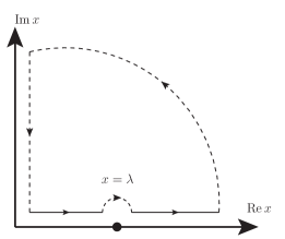
Figure 8: The contour for (67). The entire loop integrate to zero, while the solid part is the desired path.

For the second piece, one needs to take $x$ to the complex plane, and the path of integration is as shown in figure 8. One may complete the contour into a close loop as shown, which integrates to zero identically. The arc at infinity vanishes due to the Bose function. The required $c^{\prime\prime}$ is therefore the sum of the small semicircle around $x=\lambda$ and the line integral along the imaginary-$x$ axis.

The other necessary trick is to rewrite the Bose function as

$$\frac{1}{e^{x}-1}=-\frac{1}{2}+\frac{1}{x}+\sum_{k=1}^{\infty}\frac{2x}{x^{2}+(2\pi k)^{2}}.$$ (68)

and carry out the integration term by term.

The small semicircle around the $x=\lambda$ pole is easily evaluated using the residue theorem. With the aforementioned convergence factor $x^{-2\epsilon}$, the integral along the imaginary-$x$ axis and the sum over $k$ can be performed using standard $\epsilon$-expansion and $\zeta$-function regularization techniques, respectively. Individually the pieces in (68) yields $1/\epsilon$ poles, which cancel among themselves. After taking $\epsilon\rightarrow 0$, the end result is

$$\begin{split}c^{\prime\prime}(\lambda)=&\;-\frac{3}{8\pi^{2}}\Bigg{[}\frac{\pi^{2}}{3}\,+\lambda^{2}\ln|\lambda|+\lambda^{2}(\gamma_{E}-\ln 2\pi)\\ &+\lambda^{2}\sum_{n=1}^{\infty}(-1)^{n}\zeta(2n+1)\left(\frac{\lambda}{2\pi}\right)^{\!2n}\Bigg{]}.\end{split}$$ (69)

Integrating this result twice with respect to $lambda$, and imposing the condition $c(0)=c^{\prime}(0)=0$, one recovers (28) as desired.

References

- Doniach and Engelsberg (1966) S. Doniach and S. Engelsberg, Physical Review Letters 17, 750 (1966).
- Amit et al. (1968a) D. J. Amit, J. W. Kane, and H. Wagner, Physical Review 175, 326 (1968a).
- Mota et al. (1969) A. C. Mota, R. P. Platzeck, R. Rapp, and J. C. Wheatley, Physical Review 177, 266 (1969).
- Pethick and Carneiro (1973) C. J. Pethick and G. M. Carneiro, Physical Review A 7, 304 (1973).
- Carneiro and Pethick (1975) G. M. Carneiro and C. J. Pethick, Physical Review B 11, 1106 (1975).
- Carneiro and Pethick (1977) G. M. Carneiro and C. J. Pethick, Physical Review B 16, 1933 (1977).
- Belitz et al. (1997) D. Belitz, T. R. Kirkpatrick, and T. Vojta, Physical Review B 55, 9452 (1997), arXiv:9611099 [cond-mat] .
- Chitov and Millis (2001) G. Y. Chitov and A. J. Millis, Physical Review B 64, 054414 (2001), arXiv:0103155v1 [arXiv:cond-mat] .
- Misawa (2001) S. Misawa, Physica B: Condensed Matter 294-295, 10 (2001).
- Chubukov and Maslov (2003) A. V. Chubukov and D. L. Maslov, Physical Review B 68, 155113 (2003), arXiv:0305022 [cond-mat] .
- Betouras et al. (2005) J. Betouras, D. Efremov, and A. Chubukov, Physical Review B 72, 115112 (2005), arXiv:0506083 [cond-mat] .
- Chubukov et al. (2005) A. V. Chubukov, D. L. Maslov, S. Gangadharaiah, and L. I. Glazman, Physical Review Letters 95, 026402 (2005), arXiv:0502542 [cond-mat] .
- Chubukov et al. (2006) A. V. Chubukov, D. L. Maslov, and A. J. Millis, Physical Review B 73, 045128 (2006).
- Maslov and Chubukov (2009) D. L. Maslov and A. V. Chubukov, Physical Review B 79, 075112 (2009).
- Abel et al. (1966) W. R. Abel, A. C. Anderson, W. C. Black, and J. C. Wheatley, Physical Review 147, 111 (1966).
- Greywall (1983) D. S. Greywall, Physical Review B 27, 2747 (1983).
- Coffey and Pethick (1986) D. Coffey and C. J. Pethick, Physical Review B 33, 7508 (1986).
- Van Der Meulen et al. (1990) H. P. Van Der Meulen, Z. Tarnawski, A. De Visser, J. J. Franse, J. A. Perenboom, D. Althof, and H. Van Kempen, Physical Review B 41, 9352 (1990).
- Coffey and Pethick (1988) D. Coffey and C. J. Pethick, Physical Review B 37, 442 (1988).
- Vojta et al. (1997) T. Vojta, D. Belitz, R. Narayanan, and T. Kirkpatrick, Zeitschrift für Physik B Condensed Matter 103, 451 (1997).
- Belitz et al. (1999) D. Belitz, T. R. Kirkpatrick, and T. Vojta, Physical Review Letters 82, 4707 (1999), arXiv:9812420 [cond-mat] .
- Pfleiderer et al. (1997) C. Pfleiderer, G. J. McMullan, S. R. Julian, and G. G. Lonzarich, Physical Review B 55, 8330 (1997).
- Amit et al. (1968b) D. J. Amit, J. W. Kane, and H. Wagner, Physical Review 175, 313 (1968b).
- Dy and Pethick (1969) K. S. Dy and C. J. Pethick, Physical Review 185, 373 (1969).
- Baym and Pethick (1991) G. Baym and C. J. Pethick, Landau Fermi-Liquid Theory: Concepts and Applications (Wiley-VCH, 1991) p. 216.
- Zhang et al. (2009) G. M. Zhang, Y. H. Su, Z. Y. Lu, Z. Y. Weng, D. H. Lee, and T. Xiang, EPL (Europhysics Letters) 86, 37006 (2009), arXiv:0809.3874 .
- Wang et al. (2009) X. F. Wang, T. Wu, G. Wu, H. Chen, Y. L. Xie, J. J. Ying, Y. J. Yan, R. H. Liu, and X. H. Chen, Physical Review Letters 102, 100 (2009), arXiv:0806.2452 .
- Klingeler et al. (2010) R. Klingeler, N. Leps, I. Hellmann, A. Popa, U. Stockert, C. Hess, V. Kataev, H.-J. Grafe, F. Hammerath, G. Lang, S. Wurmehl, G. Behr, L. Harnagea, S. Singh, and B. Büchner, Physical Review B 81, 024506 (2010), arXiv:0808.0708 .
- Korshunov et al. (2009) M. M. Korshunov, I. Eremin, D. V. Efremov, D. L. Maslov, and A. V. Chubukov, Physical Review Letters 102, 1 (2009), arXiv:0901.0238 .
- Inouye et al. (1998) S. Inouye, M. R. Andrews, J. Stenger, H.-J. Miesner, D. M. Stamper-Kurn, and W. Ketterle, Nature 392, 151 (1998).
- Chin et al. (2010) C. Chin, R. Grimm, P. Julienne, and E. Tiesinga, Reviews of Modern Physics 82, 1225 (2010), arXiv:0812.1496 .
- Cheng and Yip (2007) C.-H. Cheng and S.-K. Yip, Physical Review B 75, 014526 (2007), arXiv:0611578 [cond-mat] .
- Navon et al. (2010) N. Navon, S. Nascimbene, F. Chevy, and C. Salomon, Science 328, 729 (2010), arXiv:1004.1465 .
- Ku et al. (2012) M. J. H. Ku, A. T. Sommer, L. W. Cheuk, and M. W. Zwierlein, Science 335, 563 (2012), arXiv:1110.3309 .
- Van Houcke et al. (2012) K. Van Houcke, F. Werner, E. Kozik, N. Prokof’ev, B. Svistunov, M. J. H. Ku, A. T. Sommer, L. W. Cheuk, A. Schirotzek, and M. W. Zwierlein, Nature Physics 8, 366 (2012), arXiv:arXiv:1110.3747v2 .
- Desbuquois et al. (2014) R. Desbuquois, T. Yefsah, L. Chomaz, C. Weitenberg, L. Corman, S. Nascimbène, and J. Dalibard, Physical Review Letters 113, 020404 (2014), arXiv:1403.4030 .
- Fukuhara et al. (2007) T. Fukuhara, Y. Takasu, M. Kumakura, and Y. Takahashi, Physical Review Letters 98, 030401 (2007), arXiv:0607228 [arXiv:cond-mat] .
- Cazalilla et al. (2009) M. A. Cazalilla, A. F. Ho, and M. Ueda, New Journal of Physics 11, 103033 (2009), arXiv:0905.4948 .
- DeSalvo et al. (2010) B. J. DeSalvo, M. Yan, P. G. Mickelson, Y. N. Martinez de Escobar, and T. C. Killian, Physical Review Letters 105, 030402 (2010), arXiv:1005.0668 .
- Cazalilla and Rey (2014) M. A. Cazalilla and A. M. Rey, Reports on Progress in Physics 77, 124401 (2014), arXiv:arXiv:1403.2792v1 .
- Cheng and Yip (2017) C.-H. Cheng and S.-K. Yip, Physical Review A 95, 033619 (2017), arXiv:1612.07886 .
- Belitz and Vojta (2005) D. Belitz and T. Vojta, Reviews of Modern Physics 77, 579 (2005).
- Note (1) For the general case of , third order terms in magnetic field is possible; see section VI. But it is also determined exclusively by FL parameters.
- Kanno (1970) S. Kanno, Progress of Theoretical Physics 44, 813 (1970).
- Luttinger and Ward (1960) J. M. Luttinger and J. C. Ward, Physical Review 118, 1417 (1960).