Distributed Approximate Newton Algorithms and Weight Design for Constrained Optimization

Abstract

Motivated by economic dispatch and linearly-constrained resource allocation problems, this paper proposes a class of novel distributed approx-Newton algorithms that approximate the standard Newton optimization method. We first develop the notion of an optimal edge weighting for the communication graph over which agents implement the second-order algorithm, and propose a convex approximation for the nonconvex weight design problem. We next build on the optimal weight design to develop a discrete distributed approx-Newton algorithm which converges linearly to the optimal solution for economic dispatch problems with unknown cost functions and relaxed local box constraints. For the full box-constrained problem, we develop a continuous distributed approx-Newton algorithm which is inspired by first-order saddle-point methods and rigorously prove its convergence to the primal and dual optimizers. A main property of each of these distributed algorithms is that they only require agents to exchange constant-size communication messages, which lends itself to scalable implementations. Simulations demonstrate that the distributed approx-Newton algorithms with our weight design have superior convergence properties compared to existing weighting strategies for first-order saddle-point and gradient descent methods.

1 Introduction

Motivation. Networked systems endowed with distributed, multi-agent intelligence are becoming pervasive in modern infrastructure systems such as power, traffic, and large-scale distribution networks. However, these advancements lead to new challenges in the coordination of the multiple agents operating the network, which are mindful of the network dynamics, and subject to partial information and communication constraints. To this end, distributed convex optimization is a rapidly emerging field which seeks to develop useful algorithms to manage network resources in a scalable manner. Motivated by the rapid emergence of distributed energy resources, a problem that has recently gained large attention is that of economic dispatch. In this problem, a total net load constraint must be satisfied by a set of generators which each have an associated cost of producing electricity. However, the existing distributed techniques to solve this problem are often limited by rate of convergence. Motivated by this, here we investigate the design of topology weighting strategies that build on the Newton method and lead to improved convergence rates.
Literature Review. The Newton method for minimizing a real-valued multivariate objective function is well characterized for centralized contexts in [3]. Another centralized method for solving general constrained convex problems by seeking the saddle-point of the associated Lagrangian is developed in [7]. This method, which implements a saddle-point dynamics is attractive because its convergence properties can be established. Other first-order or primal-dual based methods for approaching distributed optimization include [14, 8, 4, 10]. However, these methods typically do not incorporate second-order information of the cost function, which compromises convergence speeds. The notion of computing an approximate Newton direction in distributed contexts has gained popularity recently, such as [15] and [23, 24]. In the former work, the authors propose a method which uses the Taylor series expansion for inverting matrices. However, it assumes that each agent keeps an estimate of the entire decision variable, which does not scale well in problems where this variable dimension is equal to the number of agents in the network. Additionally, the optimization is unconstrained, which helps to keep the problem decoupled but is narrower in scope. The latter works pose a separable optimization with an equality constraint characterized by the incidence matrix. The proposed method may be not directly applied to networks with constraints that involve the information of all agents. The papers [12, 26, 5] incorporate multi-timescaled dynamics together with a dynamic consensus step to speed up the convergence of the agreement subroutine. These works only consider uniform edge weights, while sophisticated design of the weighting may improve the convergence. In [25], the Laplacian weight design problem for separable resource allocation is approached from a distributed gradient descent perspective. Solution post-scaling is also presented, which can be found similarly in [16] and [19] for improving the convergence of the Taylor series expression for matrix inverses. In [20], the authors consider edge weight design to minimize the spectrum of Laplacian matrices. However, in the Newton descent framework, the weight design problem formulates as a nonconvex bilinear problem, which is challenging to solve. Overall, the current weight-design techniques that are computable in polynomial time are only mindful of first-order algorithm dynamics. A second-order approach has its challenges, which manifest themselves in a bilinear design problem and more demanding communication requirements, but using second-order information is more heedful of the problem geometry and leads to faster convergence speeds.

Statement of Contributions. In this paper, we propose a novel framework to design a weighted Laplacian matrix that is used in the solution to a multi-agent optimization problem via sparse approximated Newton algorithms. Motivated by economic dispatch, we start by formulating a separable resource allocation problem subject to a global linear constraint and local box constraints, and then derive an equivalent form without the global constraint by means of a Laplacian matrix, which is well suited for a distributed framework. We use this to motivate weighting design of the elements of the Laplacian matrix and formulate this problem as a bilinear optimization. We develop a convex approximation of this problem whose solution can be computed offline in polynomial time. A bound on the best-case solution of the original bilinear problem is also given.

We aim to bridge the gap between classic Newton and distributed approx-Newton methods. To do this, we first relax the box constraints and develop a class of constant step-size discrete-time algorithms. The Newton step associated with the unconstrained optimization problem do not inherit the same sparsity as the distributed communication network. To address this issue, we consider approximations based on a Taylor series expansion, where the first few terms inherit certain level of sparsity as prescribed by the Laplacian matrix. We analyze the approximate algorithms and show their convergence for any truncation of the series expansion.

We next study the original problem with local box constraints, which has never been considered in the framework of a distributed Newton method, and present a novel continuous-time distributed approx-Newton algorithm. The convergence of this algorithm to the optimizer is rigorously studied and we give an interpretation of the convergence in the Lyapunov function sense. Furthermore, through a formal statement of the proposed distributed approx-Newton algorithm (or DANA), we find several interesting insights on second-order distributed methods. We compare the results of our design and algorithm to a generic weighting design of distributed gradient descent (DGD) implementations in simulation. Our weighting design shows superior convergence to DGD.

Organization. The rest of the paper is organized as follows. Section 2 introduces the notations and fundamentals used in this paper. We formulate the optimal resource allocation problem in Section 3. Section 4 proposes the optimal graph weighting design for a second order method and develops a convex approximation to compute a satisfactory solution. In Section 5, we propose a distributed algorithm that approximates the Newton step in solving the optimization. Section 7 demonstrates the effectiveness of the proposed algorithm. We conclude the paper in Section 8.

2 Preliminaries

This section compiles notation and presents a few results that will be used in the sequel.

2.1 Notation

Let $\mathbb{R}$ and $\mathbb{R}_{+}$ denote the set of real and positive real numbers, respectively, and let ${\mathbb{N}}$ denote the set of natural numbers. For a vector ${x\in\mathbb{R}^{n}}$, we denote by $x_{i}$ the $i^{\textup{th}}$ entry of $x$. For a matrix ${A\in\mathbb{R}^{n\times m}}$, we write $A_{i}$ as the $i^{\textup{th}}$ row of $A$ and $A_{ij}$ as the element in the $i^{\textup{th}}$ row and $j^{\textup{th}}$ column of $A$. Discrete time-indexed variables are written as $x^{k}$, where $k$ denotes the current time step. The transpose of a vector or matrix is denoted by $x^{\top}$ and $A^{\top}$, respectively. We use the shorthand notations ${\mathbf{1}_{n}=[1,\dots,1]^{\top}\in\mathbb{R}^{n}}$, ${\boldsymbol{0}_{n}=[0,\dots,0]^{\top}\in\mathbb{R}^{n}}$, and $I_{n}$ to denote the ${n\times n}$ identity matrix. The standard inner product of two vectors $x,y\in\mathbb{R}^{n}$ is written $\langle x,y\rangle$, and $x\perp y$ indicates $\langle x,y\rangle=0$. For a real-valued function ${f:\mathbb{R}^{n}\rightarrow\mathbb{R}}$, the gradient vector of $f$ with respect to $x$ is denoted by ${\nabla_{x}f(x)}$ and the Hessian matrix with respect to $x$ by ${\nabla_{xx}f(x)}$. The positive (semi) definiteness and negative (semi) definiteness of a matrix ${A\in\mathbb{R}^{n\times n}}$ is indicated by ${A\succ 0}$ and ${A\prec 0}$ (resp. ${A\succeq 0}$ and ${A\preceq 0}$). The same symbols are used to indicate componentwise inequalities on vectors of equal sizes. The set of eigenvalues of a symmetric matrix ${A\in\mathbb{R}^{n\times n}}$ is ordered as $\mu_{1}(A)\leq\dots\leq\mu_{n}(A)$ with associated eigenvectors $v_{1},\dots,v_{n}\in\mathbb{R}^{n}$. An orthogonal matrix ${T\in\mathbb{R}^{n\times n}}$ has the property ${T^{\top}T=TT^{\top}=I_{n}}$ and ${T^{\top}=T^{-1}}$. For a finite set $\mathcal{S}$, $|\mathcal{S}|$ is the cardinality of the set. The uniform distribution on the interval $[a,b]$ is indicated by $\mathcal{U}[a,b]$. We define the projection

$$\left[u\right]^{+}_{v}:=\begin{cases}u,&v>0,\\ \text{max}\{0,u\},&v\leq 0.\end{cases}$$

2.2 Graph Theory

A network of agents is represented by a graph $\operatorname{\mathcal{G}}=(\operatorname{\mathcal{N}},\mathcal{E})$, assumed undirected, with a node set $\operatorname{\mathcal{N}}=\{1,\dots,n\}$ and edge set $\mathcal{E}\subseteq\operatorname{\mathcal{N}}\times\operatorname{\mathcal{N}}$. The edge set $\mathcal{E}$ has elements $(i,j)\in\mathcal{E}$ for $j\in\operatorname{\mathcal{N}}_{i}$, where $\operatorname{\mathcal{N}}_{i}\subset\operatorname{\mathcal{N}}$ is the set of neighbors of agent $i\in\operatorname{\mathcal{N}}$. The union of neighbors to each agent $j\in\operatorname{\mathcal{N}}_{i}$ are the 2-hop neighbors of agent $i$, and denoted by $\operatorname{\mathcal{N}}_{i}^{2}$. More generally, $\operatorname{\mathcal{N}}_{i}^{p}$, or set of $p$-hop neighbors of $i$, is the union of neighbors of agents in $\operatorname{\mathcal{N}}_{i}^{p-1}$. We consider weighted edges for the sake of defining the graph Laplacian; the role of edge weightings and the associated design problem in this paper is described in Section 4. The graph $\operatorname{\mathcal{G}}$ then has a weighted Laplacian ${L\in\mathbb{R}^{n\times n}}$ defined as

$$L_{ij}=\begin{cases}-w_{ij},&j\in\operatorname{\mathcal{N}}_{i},j\neq i,\\ w_{ii},&j=i,\\ 0,&\text{otherwise},\end{cases}$$

with weights $w_{ij}=w_{ji}>0,\forall j\neq i$, and total incident weight $w_{ii}$ on $i\in\operatorname{\mathcal{N}}$, ${w_{ii}=\sum_{j\in\operatorname{\mathcal{N}}_{i}}w_{ij}}$. Evidently, $L$ has an eigenvector ${v_{1}=\boldsymbol{1}_{n}}$ with an associated eigenvalue ${\mu_{1}=0}$, and ${L=L^{\top}\succeq 0}$. The graph is connected i.f.f. $0$ is a simple eigenvalue, i.e. $0=\mu_{1}<\mu_{2}\leq\dots\leq\mu_{n}$.

The Laplacian $L$ can be written via its incidence matrix ${E\in\{-1,0,1\}^{|\mathcal{E}|\times n}}$ and a diagonal matrix ${X\in\mathbb{R}_{+}^{|\mathcal{E}|\times|\mathcal{E}|}}$ whose entries are weights $w_{ij}$. Each row of $E$ is associated with an edge $(i,j)$ whose $i^{\textup{th}}$ element is $1$, $j^{\textup{th}}$ element is $-1$, and all other elements zero. Then, $L=E^{\top}XE$.

2.3 Schur Complement

The following lemma will be used in the sequel.

Lemma 1.

[27](Matrix Definiteness via Schur Complement). Consider a symmetric matrix $M$ of the form

$$M=\begin{bmatrix}A&B\\ B^{\top}&C\end{bmatrix}.$$

If $C$ is invertible, then the following properties hold:
(1) $M\succ 0$ if and only if $C\succ 0$ and $A-BC^{-1}B^{\top}\succ 0$.
(2) If $C\succ 0$, then $M\succeq 0$ if and only if $A-BC^{-1}B^{\top}\succeq 0$.

2.4 Taylor Series Expansion for Matrix Inverses

A full-rank matrix $A\in\mathbb{R}^{n\times n}$ has a matrix inverse, $A^{-1}$, which is characterized by the relation $AA^{-1}=I_{n}$. In principle, it is not straightforward to compute this inverse via a distributed algorithm. However, if the eigenvalues of $A$ satisfy $|1-\mu_{i}(A)|<1,\forall\,i\in\mathcal{N}$, then we can employ the Taylor expansion to compute its inverse [21]:

$$A^{-1}=\sum_{p=0}^{\infty}(I_{n}-A)^{p}.$$

To quickly see this holds, substitute $B=I_{n}-A$, multiply both sides by $I_{n}-B$ and reason with $\lim_{p\rightarrow\infty}$. Note that, if the sparsity structure of $A$ represents a network topology, then traditional matrix inversion techniques such as Gauss-Jordan elimination still necessitate all-to-all communication. However, agents can communicate and compute locally to obtain each term in the previous expansion. If $A$ is normal, it can be seen via the diagonalization of $I_{n}-A$ that the terms of the sum become small as $p$ increases due to the assumption on the eigenvalues of $A$ [9]. The convergence of these terms is exponential and limited by the slowest converging mode, i.e. $\max{|1-\mu_{i}(A)|}$.

We can compute an approximation of $A^{-1}$ in finite steps by computing and summing the terms up to the $q^{\textup{th}}$ power. We refer to this approximation as a q-approximation of $A^{-1}$.

3 Problem Statement

Motivated by the economic dispatch problem, in this section we pose the separable resource allocation problem that we aim to solve distributively. We reformulate it as an unconstrained optimization problem whose decision variable is in the span of the graph Laplacian, and motivate the characterization of a second-order Newton-inspired method.

Consider a group of agents $\operatorname{\mathcal{N}}$, indexed by $i\in\operatorname{\mathcal{N}}$, and a communication topology given by $\operatorname{\mathcal{G}}$. Each agent is associated with a local convex cost function $f_{i}:\mathbb{R}\rightarrow\mathbb{R}$. These agents can be thought of as generators in an electricity market, where each function argument $x_{i}\in\mathbb{R}$, $i\in\operatorname{\mathcal{N}}$ represents the power that agent $i$ produces at a cost characterized by $f_{i}$. The economic dispatch problem aims to satisfy a global load-balancing constraint $\sum_{i=1}^{n}x_{i}=d$ for minimal global cost $f:\mathbb{R}^{n}\rightarrow\mathbb{R}$, where $d$ is the total demand. In addition, each agent is subject to a local linear box constraint on its decision variable given by the interval $[\underline{x}_{i},\overline{x}_{i}]$. Then, the economic dispatch optimization problem is stated as:

$${\mathcal{P}}1:\ \underset{x}{\text{min}} f(x)=\sum_{i=1}^{n}f_{i}(x_{i})$$ (1a)

subject to $$\sum_{i=1}^{n}x_{i}=d,$$ (1b)

$$\underline{x}_{i}\leq x_{i}\leq\overline{x}_{i},\quad i=\{1,\dots,n\}.$$ (1c)

Distributed optimization algorithms based on a gradient descent approach to solve ${\mathcal{P}}1$ are available [28]. However, by only taking into account first-order information of the cost functions, these methods tend to be inherently slow. As for a Newton (second-order) method, the constraints make the computation of the descent direction non-distributed. To see this, consider only (1a)–(1b). Recall the unconstrainted Newton step defined as $x_{\textup{nt}}:=-\nabla_{xx}f(x)^{-1}\nabla_{x}f(x)$, see e.g. [3]. In this context, the equality constraint can be eliminated by imposing ${x_{n}=d-\sum_{i=1}^{n-1}x_{i}}$. Then, (1a) becomes ${f(x)=\sum_{i=1}^{n-1}f_{i}(x_{i})+f_{n}(d-\sum_{i=1}^{n-1}x_{i})}$. In general, the resulting Hessian $\nabla_{xx}f(x)$ is fully populated and its inverse requires all-to-all communication among agents in order to compute the second-order descent direction. If we additionally consider (1c), interior point methods are often employed, such as introducing a log-barrier function to the cost in (1a)[3]. The value of the log-barrier parameter is updated online to converge to a feasible solution, which exacerbates the non-distributed nature of this approach. This motivates the design of distributed Newton-like methods which are cognizant of (1b)–(1c).

We eliminate (1b) by introducing a network topology as encoded by a Laplacian matrix $L$ associated with $\operatorname{\mathcal{G}}$ and an initial condition $x^{0}\in\mathbb{R}^{n}$ with some assumptions.

Assumption 1.

(Undirected and Connected Graph). The weighted graph characterized by $L$ is undirected and connected, i.e. $L=L^{\top}$ and $0$ is a simple eigenvalue of $L$.

Assumption 2.

(Feasible Initial Condition). The initial state $x^{0}$ satisfies (1b), i.e.

$$\sum_{i=1}^{n}x_{i}^{0}=d.$$

If the problem context does not lend itself well to satisfying Assumption 2, there is a distributed algorithmic solution to rectify this via dynamic consensus that can be found in [6] which could be modified for a Newton-like method. Given these assumptions, ${\mathcal{P}}1$ is equivalent to:

$${\mathcal{P}}2:\ \underset{z}{\text{min}} f(x^{0}+Lz)=\sum_{i=1}^{n}f_{i}(x^{0}_{i}+L_{i}z)$$ (2a)

subject to $$\underline{x}-x^{0}-Lz\preceq\boldsymbol{0}_{n},$$ (2b)

$$x^{0}+Lz-\overline{x}\preceq\boldsymbol{0}_{n}.$$ (2c)

Using the property that $\boldsymbol{1}_{n}$ is an eigenvector of $L$ associated with the eigenvalue $0$, we have that $\boldsymbol{1}_{n}^{\top}(x^{0}+Lz)=d$. Newton descent for centralized solvers is given in [3]; in our distributed framework, the row space of the Laplacian is a useful property to address (1b).

Remark 1.

(Relaxing Assumption 2). The assumption on the initial condition can render the formulation vulnerable to implementation errors and cannot easily accommodate packet drops in a distributed algorithm. A potential workaround for this is outlined here. Consider, instead of (1b) in ${\mathcal{P}}1$, the $n$ linear constraints:

$$x+Lz=\overline{d},$$ (3)

where $\overline{d}\in\mathbb{R}^{n},\boldsymbol{1}_{n}^{\top}\overline{d}=d$ and (1b) can be recovered by multiplying (3) from the left by $\boldsymbol{1}_{n}$. (As an aside, it may be desirable to impose sparsity on $\overline{d}$ so that only some agents need access to global problem data). Both $x\in\mathbb{R}^{n}$ and $z\in\mathbb{R}^{n}$ become decision variables, and agent $i$ can verify the $i^{\textup{th}}$ component of (3) with one-hop neighbor information. Further, a distributed saddle-point algorithm can be obtained by assigning a dual variable to (3) and proceeding as in [7].

We provide a simulation justification for this approach in Section 7.4, although the analysis of robustness to perturbations and packet drops is ongoing and outside the scope of this paper. For now we strictly impose Assumption 2.

We aim to leverage the freedom given by the elements of $L$ in order to compute an approximate Newton direction to ${\mathcal{P}}2$. To this end, we adopt the following assumption.

Assumption 3.

(Cost Functions). The local costs $f_{i}$ are twice continuously differentiable and strongly convex with bounded second-derivatives given by

$$0<\delta_{i}\leq\dfrac{\partial^{2}f_{i}}{\partial x_{i}^{2}}\leq\Delta_{i},$$

for every $i\in\operatorname{\mathcal{N}}$ with given $\delta_{i},\Delta_{i}\in\mathbb{R}_{+}$.

This assumption is common in other distributed Newton or Newton-like methods, e.g. [15, 12] and in classical convex optimization [3, 17]. Assumption 3 is necessary to attain convergence in our computation of the Newton step/direction and to construct the notion of an optimal edge weighting $L$. We adopt the shorthands $H(x):=\nabla_{xx}f(x)$, $H_{\delta}:=\operatorname{diag}(\delta)$, and $H_{\Delta}:=\operatorname{diag}(\Delta)$ as the diagonal matrices with elements given by $\partial^{2}f_{i}(x_{i})/\partial x_{i}^{2}$, $\delta_{i}$, and $\Delta_{i}$, respectively.

Next, for the purpose of developing a distributed Newton-like method, we must slightly rethink the idea of inverting a Hessian matrix. By application of the chain rule, we have that $\nabla_{zz}f(x^{0}+Lz)=LH(x^{0}+Lz)L$. Clearly, $\nabla_{zz}f$ is non-invertible due to the smallest eigenvalue of $L$ fixed at zero, a manifestation of the equality constraint in the original problem ${\mathcal{P}}1$. We instead focus on the $n-1$ nonfixed eigenvalues of $\nabla_{zz}f$ to employ the Taylor expansion outlined in Section 2.4. To this end, we project $LH(x^{0}+Lz)L$ to the $\mathbb{R}^{(n-1)\times(n-1)}$ space with a coordinate transformation; the justification for this and relation to the traditional Newton method are made explicitly clear in Section 5. We seek a matrix $T\in\mathbb{R}^{n\times n}$ satisfying $T^{\top}T=I_{n}-\boldsymbol{1}_{n}\boldsymbol{1}_{n}^{\top}/n$ [9]; the particular matrix $T$ we employ is given as

$$T=\begin{bmatrix}n-1+\sqrt{n}&-1&\cdots&-1&\dfrac{1}{\sqrt{n}}\\ -1&\ddots&\cdots&\vdots&\\ \vdots&&\ddots&-1&\vdots\\ -1&\cdots&-1&n-1+\sqrt{n}&\\ -1-\sqrt{n}&\cdots&\cdots&-1-\sqrt{n}&\dfrac{1}{\sqrt{n}}\end{bmatrix}\operatorname{diag}(\begin{bmatrix}\rho\\ 1\end{bmatrix}),$$

where $\rho=\sqrt{n(n+1+2\sqrt{n})}^{-1}\boldsymbol{1}_{n-1}$. This choice of $T$ has the effect of projecting the null-space of the Hessian onto the $n^{\textup{th}}$ row and $n^{\textup{th}}$ column, which is demonstrated by defining $M(x):=JT^{\top}LH(x)LTJ^{\top}\in\mathbb{R}^{(n-1)\times(n-1)}$, where $J=\begin{bmatrix}I_{n-1}&\boldsymbol{0}_{n-1}\end{bmatrix}$. The matrix $M(x)$ shares its $n-1$ eigenvalues with the $n-1$ nonzero eigenvalues of $LH(x)L$ at each $x$, and $M(x)^{-1}$ is well defined, which provides us with a concrete notion of an inverse Hessian. We now adopt the following assumption.

Assumption 4.

(Convergent Eigenvalues). For any $x$, the eigenvalues of $I_{n-1}-M(x)$, corresponding to the $n-1$ smallest eigenvalues of $I_{n}-LH(x)L$, are contained in the unit ball, i.e. $\exists\ \varepsilon<1$ such that

$$-\varepsilon I_{n-1}\preceq I_{n-1}-M(x)\preceq\varepsilon I_{n-1}.$$

Technically speaking, we are only concerned with arguments of $M$ belonging to the $n-1$ dimensional hyperplane $\{x^{0}+Lz\;|\;z\in\mathbb{R}^{n}\}$, although we consider all $x\in\mathbb{R}^{n}$ for simplicity. In the following section, we address Assumption 4 (Convergent Eigenvalues) by minimizing $\varepsilon$ via weight design of the Laplacian. By doing this, we aim to obtain a good approximation of $M^{-1}$ from the Taylor expansion with small $q$, which lends itself well to the convergence of the distributed algorithms in Sections 5 and 6.

4 Weight Design of the Laplacian

In this section, we pose the nonconvex weight design problem on the elements of $L$, which formulates as a bilinear optimization to be solved by a central authority. To make this problem tractable, we develop a convex approximation and demonstrate that the solution is guaranteed to satisfy Assumption 4. Next, we provide a lower bound on the solution to the nonconvex problem. This gives a measure of performance for evaluating our approximation.

4.1 Formulation and Convex Approximation

Our approach hearkens to the intuition on the rate of convergence of the $q$-approximation of $M(x)^{-1}$. We design a weighting scheme for a communication topology characterized by $L$ which lends itself to a scalable, fast approximation of a Newton-like direction. To this end, we minimize $\underset{i,x}{\max}|1-\mu_{i}(M(x))|$:

$${\mathcal{P}}3:\quad \underset{\varepsilon,L}{\text{min}} \varepsilon$$ (4a)

s.t. $$-\varepsilon I_{n-1}\preceq I_{n-1}-M(x)\preceq\varepsilon I_{n-1},\forall x,$$ (4b)

$$L\boldsymbol{1}_{n}=\boldsymbol{0}_{n},\ L\succeq 0,\ L=L^{\top},$$ (4c)

$$L_{ij}\leq 0,j\in\operatorname{\mathcal{N}}_{i},\ L_{ij}=0,\,j\notin\operatorname{\mathcal{N}}_{i}.$$ (4d)

Naturally, ${\mathcal{P}}3$ must be solved offline by a central authority because it requires complete information about the local Hessians embedded in $M(x)$, in addition to being a semidefinite program for which distributed solvers are not mature. Even for a centralized solver ${\mathcal{P}}3$ is hard for a few reasons, the first being that (4b) is a function over all possible $x\in\mathbb{R}^{n}$. To reconcile with this, we invoke Assumption 3 on the cost functions and write $M_{\delta}=JT^{\top}LH_{\delta}LTJ^{\top}$ and $M_{\Delta}=JT^{\top}LH_{\Delta}LTJ^{\top}$. Then, (4b) is equivalent to

$$-(\varepsilon_{-}+1)I_{n-1}+M_{\delta} \preceq 0,$$ (5a)

$$(1-\varepsilon_{+})I_{n-1}-M_{\Delta} \preceq 0,$$ (5b)

$$\varepsilon_{-}=\varepsilon_{+},$$ (5c)

where the purpose of introducing $\varepsilon_{-}$ and $\varepsilon_{+}$ will become clear in the discussion that follows.

The other difficult element of ${\mathcal{P}}3$ is the nonconvexity stemming from (5a)–(5b) being bilinear in $L$. There are path-following techniques available to solve bilinear problems of this form [11], but simulation results do not produce satisfactory solutions for problems of the form ${\mathcal{P}}3$. Instead, we aim to develop a convex approximation of ${\mathcal{P}}3$ which exploits its structure. Consider (5a) and (5b) separately by relaxing (5c). In fact, (5a) may be rewritten in a convex manner. To do this, write $L$ as a weighted product of its incidence matrix, $L=E^{\top}XE$. Applying Lemma 1 makes the constraint become

$$\begin{bmatrix}(\varepsilon_{-}+1)I_{n-1}&JT^{\top}E^{\top}XE\\ E^{\top}XETJ^{\top}&H_{\delta}^{-1}\end{bmatrix}\succeq 0.$$ (6)

As for (5b), consider the approximation $LH_{\Delta}L\approx\left(\dfrac{\sqrt{H_{\Delta}}L+L\sqrt{H_{\Delta}}}{2}\right)^{2}$. This approximation can be thought of as a rough completion of squares, which lends itself well to our approach of convexifying (5b). One should not expect the approximation to be reliably “better” or “worse” than the BMI; rather, it is only intended to reflect the original constraint more than a simple linearization. To this end, substitute this in $M_{\Delta}$ to get

$$\dfrac{1}{4}JT^{\top}(\sqrt{H_{\Delta}}L+L\sqrt{H_{\Delta}})^{2}TJ^{\top}\succeq(1-\varepsilon_{+})I_{n-1}$$

$$\dfrac{1}{2}JT^{\top}(\sqrt{H_{\Delta}}L+L\sqrt{H_{\Delta}})TJ^{\top}\succeq\sqrt{(1-\varepsilon_{+})}I_{n-1}$$

$$\dfrac{1}{2}JT^{\top}(\sqrt{H_{\Delta}}L+L\sqrt{H_{\Delta}})TJ^{\top}\succeq$$

$$\hskip 99.58464pt(1-\dfrac{\varepsilon_{+}}{2}+\dfrac{\varepsilon_{+}^{2}}{8}+O(\varepsilon_{+}^{3}))I_{n-1},$$

where the second line uses the property that $TJ^{\top}JT^{\top}=I_{n}-\boldsymbol{1}_{n}\boldsymbol{1}_{n}^{\top}/n$ is idempotent and that

$$\left(\dfrac{1}{2}JT^{\top}(\sqrt{H_{\Delta}}L+L\sqrt{H_{\Delta}})TJ^{\top}\right)^{2} \succeq(1-\varepsilon_{+})I_{n-1}$$

$$\qquad\qquad\succeq 0$$

$$\Leftrightarrow\dfrac{1}{2}JT^{\top}(\sqrt{H_{\Delta}}L+L\sqrt{H_{\Delta}})TJ^{\top} \succeq\sqrt{1-\varepsilon_{+}}I_{n-1}\succeq 0,$$

see [22]. The third line expresses the right-hand side as a Taylor expansion about $\varepsilon_{+}=0$. Neglecting the higher order terms $O(\varepsilon_{+}^{3})$ and applying Lemma 1 gives

$$\begin{bmatrix}\bullet&\dfrac{1}{\sqrt{8}}\varepsilon_{+}I_{n-1}\\ \dfrac{1}{\sqrt{8}}\varepsilon_{+}I_{n-1}&I_{n-1}\end{bmatrix}\succeq 0,$$ (7)

with ${\bullet=\dfrac{1}{2}JT^{\top}(\sqrt{H_{\Delta}}L+L\sqrt{H_{\Delta}})TJ^{\top}}-{(1-\dfrac{1}{2}\varepsilon_{+})I_{n-1}}$.

Returning to ${\mathcal{P}}3$, note that the latter three constraints are satisfied by $L=E^{\top}XE$. Then, the approximate reformulation of ${\mathcal{P}}3$ can be written as

$${\mathcal{P}}4: \underset{\varepsilon_{-},\varepsilon_{+},X}{\text{min}} \max(\varepsilon_{-},\varepsilon_{+})$$

s.t. $$\varepsilon_{-}\geq 0,\varepsilon_{+}\geq 0,$$

$$X\succeq 0,\eqref{ineq:convex_constraint},\eqref{ineq:nonconvex_constraint}.$$

This is a convex problem in $X$ and solvable in polynomial time. To improve the solution, we perform some post-scaling. Take $L^{\star}_{0}=E^{\top}X_{0}^{\star}E$, where $X_{0}^{\star}$ is the solution to ${\mathcal{P}}4$, and let $M_{\Delta 0}^{\star}=JT^{\top}L^{\star}_{0}H_{\Delta}L^{\star}_{0}TJ^{\top},M_{\delta 0}^{\star}=JT^{\top}L^{\star}_{0}H_{\delta}L^{\star}_{0}TJ^{\top}$. Then, consider

$$\beta=\sqrt{\dfrac{2}{\mu_{1}(M_{\delta 0}^{\star})+\ \mu_{n-1}(M_{\Delta 0}^{\star})}},$$

and take $L^{\star}=\beta L^{\star}_{0}$. This shifts the eigenvalues of $M^{\star}_{0}(x)$ to $M^{\star}(x)$ (defined similarly via $L^{\star}$) such that $1-\mu_{1}(M_{\delta}^{\star})=-(1-\mu_{n-1}(M_{\Delta}^{\star}))$, which shrinks $\underset{i,x}{\max}(|1-\mu_{i}(M^{\star}(x))|)$. We refer to this metric as $\varepsilon_{L^{\star}}:=\underset{i,x}{\max}(|1-\mu_{i}(M^{\star}(x))|)$, and it can be verified that this post-scaling satisfies Assumption 4 with regard to $\varepsilon_{L^{\star}}$. To see this, first consider scaling $L$ by an arbitrarily small constant, which places the eigenvalues of $I_{n-1}-M(x)$ very close to $1$ and satisfies Assumption 4. Then, consider gradually increasing this constant until the lower bound on the minimum eigenvalue and upper bound on the maximum eigenvalue of $I_{n-1}-M(x)$ are equal in magnitude. This is precisely the scaling produced by $\beta$. Then, the solution to ${\mathcal{P}}4$ followed by a post scaling by $\beta$ given by $L^{\star}$ is an approximation of the solution to the nonconvex problem ${\mathcal{P}}3$ with the sparsity structure preserved.

Remark 2.

(Unknown Local Hessian Bounds). It may be the case that a central entity tasked with computing some $L^{\star}$ does not have access to the local bounds $\delta_{i},\Delta_{i},\forall i$. In this case, globally known bounds $\delta\leq\delta_{i},\Delta_{i}\leq\Delta,\forall i$ can be substituted in place of the local values in the formulation of ${\mathcal{P}}4$. It can be verified that this will result in a more conservative formulation, and that the resulting $L^{\star}$ will still satisfy Assumption 4 at the expense of possibly larger $\varepsilon$.

4.2 A Bound on Performance

We are motivated to find a “best-case scenario” for our solution given the structural constraints of the network. Instead of solving ${\mathcal{P}}3$ for $L$, we solve it for some $A$ where $A_{ij}=0$ for $j\notin\operatorname{\mathcal{N}}_{i}^{2}$, i.e. the two-hop neighbor structure of the network and sparsity structure of $LH(x)L$. Define $M_{A}:=JT^{\top}ATJ^{\top}$. This problem is:

$${\mathcal{P}}5: \underset{\varepsilon,A}{\text{min}} \varepsilon$$

s.t. $$-\varepsilon I_{n-1}\preceq I_{n-1}-M_{A}\preceq\varepsilon I_{n-1},$$

$$A\boldsymbol{1}_{n}=\boldsymbol{0}_{n},\ A\succeq 0,$$

$$A_{ij}=0,j\notin\operatorname{\mathcal{N}}^{2}_{i}.$$

This problem is convex in $A$ and produces a solution $\varepsilon_{A}$, which serves as a lower bound for the solution to ${\mathcal{P}}3$. It should not be expected that this lower bound is tight or achievable by “reverse engineering” an $L^{\star}$ with the desired sparsity from the solution $A^{\star}$ to ${\mathcal{P}}5$, rather, $\varepsilon_{L^{\star}}-\varepsilon_{A}$ gives just a rough indication of how close $\varepsilon_{L^{\star}}$ is to the conservative lower bound of ${\mathcal{P}}3$.

5 Discrete Time Algorithm for Relaxed Economic Dispatch

In this section, we focus on a relaxed version of ${\mathcal{P}}2$ to develop a direct relation between traditional discrete-time Newton descent and our distributed, approximate method. First, we state the relaxed problem and define the approximate Newton step. We then state the discrete distributed approx-Newton algorithm and provide a rigorous study of its convergence properties.

5.1 Characterization of the Approximate Newton Step

Even the traditional centralized Newton method is not well-suited to solve ${\mathcal{P}}1$ due to the box constraints (1c). For this reason, for now we focus on the relaxed problem

$${\mathcal{P}}6:\ \underset{x}{\text{min}} f(x)=\sum_{i=1}^{n}f_{i}(x_{i}),$$ (8a)

subject to $$\sum_{i=1}^{n}x_{i}=d.$$ (8b)

The equivalent unconstrained problem in $z$ is

$${\mathcal{P}}7:\ \underset{z}{\text{min}}\quad g(z):=f(x^{0}+Lz)=\sum_{i=1}^{n}f_{i}(x^{0}_{i}+L_{i}z).$$ (9)

Remark 3.

(Nonuniqueness of Solution). Given a $z^{\star}$ which solves ${\mathcal{P}}7$, the set of solutions can be characterized by $\{z^{\star\prime}\;|\;z^{\star\prime}=z^{\star}+\gamma\boldsymbol{1}_{n}\,\ \gamma\in\mathbb{R}\}$. The fact that $z^{\star\prime}$ is a solution is due to $\operatorname{null}{(L)}=\operatorname{span}{(\boldsymbol{1}_{n})}$, and the fact that this characterizes the entire set of solutions is due to $\operatorname{null}{(\nabla_{zz}g(z))}=\operatorname{span}{(\boldsymbol{1}_{n})}$.

To solve ${\mathcal{P}}6,$ we aim to implement a descent method in $x$ via the dynamics

$$x^{+}=x+\alpha L\tilde{z}_{\textup{nt}},$$ (10)

where $\tilde{z}_{\textup{nt}}$ is the approximate Newton step that we seek to compute distributively, and $\alpha>0$ is a fixed step size.

It is true that ${\mathcal{P}}7$ is unconstrained with respect to $z$, although we have already alluded to the fact that the Hessian matrix $\nabla_{zz}g(z)=LH(x+Lz)L$ is rank-deficient stemming from (8b). We now reconcile this by deriving a well defined Newton step in a reduced variable $\hat{z}\in\mathbb{R}^{n-1}$. Consider a change of coordinates by the orthogonal matrix $T$ defined in Section 3 and write $z=TJ^{\top}\hat{z}$. Taking the gradient and Hessian of $g(z)$ with respect to $\hat{z}$ gives

$$\nabla_{\hat{z}}g(z) =JT^{\top}\nabla_{z}g(z)=JT^{\top}L\nabla_{x}f(x+LTJ^{\top}\hat{z})$$

$$\nabla_{\hat{z}\hat{z}}g(z) =JT^{\top}LH(x+LTJ^{\top}\hat{z})LTJ^{\top}$$

$$=M(x+LTJ^{\top}\hat{z}).$$

Notice that the zero eigenvalue of $\nabla_{zz}g(z)$ is eliminated by this projection and the other eigenvalues are preserved. Evaluating at $x+LTJ^{\top}\hat{z}\big{|}_{\hat{z}=0}$, the Newton step in $\hat{z}$ is now well defined as $\hat{z}_{\textup{nt}}:=-\nabla_{\hat{z}\hat{z}}g(0)^{-1}\nabla_{\hat{z}}g(0)=-M(x)^{-1}JT^{\top}L\nabla_{x}f(x)$.

Consider now a $q$-approximation of $M(x)^{-1}$ given by $\sum_{p=0}^{q}(I_{n-1}-M(x))^{p}$ and return to the original coordinates to obtain the approximate Newton direction $L\tilde{z}_{nt}$:

$$L\tilde{z}_{nt}=-LTJ^{\top}\sum_{p=0}^{q}(I_{n-1}-M(x))^{p}JT^{\top}L\nabla_{x}f(x).$$

With the property that $LTJ^{\top}JT^{\top}L=L^{2}$, rewrite $L\tilde{z}_{\textup{nt}}$:

$$L\tilde{z}_{\textup{nt}}=-L\sum_{p=0}^{q}(I_{n}-LH(x)L)^{p}L\nabla_{x}f(x).$$ (11)

It can be seen via eigendecomposition of $I_{n}-LHL$, which is normal, and application of Assumption 4 that the terms $L(I_{n}-LHL)^{p}$ become small with $p\rightarrow\infty$ at a rate dictated by $\varepsilon$. Note that there is a nonconverging mode of the sum corresponding to the eigenspace spanned by $\boldsymbol{1}_{n}$, but this is mapped to zero by left multiplication by $L$. This expression can be computed distributively: each multiplication by $L$ encodes a communication with the neighbor set of each agent, and we utilize recursion to perform the computation efficiently, which is formally described in Algorithm 1.

5.2 The distributed approx-Newton Algorithm

We now have the tools to introduce the
discrete distributed approx-Newton algorithm, or DANA-D.

Algorithm 1 $\textsc{DANA-D}_{i}$

1:$L_{ij}$ for $j\in\{i\}\cup\operatorname{\mathcal{N}}_{i}$ and communication with nodes $j\in\operatorname{\mathcal{N}}_{i}\cup\operatorname{\mathcal{N}}_{i}^{2}$

2:procedure Newton_i($x_{i}^{0},L_{i},f_{i},q$)

3:     Initialize $x_{i}\leftarrow x_{i}^{0}$

4:     loop

5:         Compute $\dfrac{\partial f_{i}}{\partial x_{i}}$, $\dfrac{\partial^{2}f_{i}}{\partial x_{i}^{2}}$; send to $j\in\operatorname{\mathcal{N}}_{i}$, $\operatorname{\mathcal{N}}^{2}_{i}$

6:         $y_{i}\leftarrow L_{ii}\dfrac{\partial f_{i}}{\partial x_{i}}+\sum_{j\in\operatorname{\mathcal{N}}_{i}}L_{ij}\dfrac{\partial f_{j}}{\partial x_{j}}$

7:         $z_{i}\leftarrow-y_{i}$

8:         $p_{i}\leftarrow 1$

9:         while $p_{i}\leq q$ do

10:              Acquire $y_{j}$ from $j\in\operatorname{\mathcal{N}}_{i}^{2}$

11:              $w_{i}=(I_{n}-LH(x)L)_{i}y$

12:              $y_{i}\leftarrow w_{i}$

13:              $z_{i}\leftarrow z_{i}-y_{i}$

14:              $p_{i}\leftarrow p_{i}+1$

15:         end while

16:         Acquire $z_{j}$ for $j\in\operatorname{\mathcal{N}}_{i}$

17:         $x_{i}\leftarrow x_{i}+\alpha\left(L_{ii}z_{i}+\sum_{j\in\operatorname{\mathcal{N}}_{i}}L_{ij}z_{j}\right)$

18:     end loop

19:     return $x_{i}$

20:end procedure

The algorithm is constructed directly from (10) and (11). The $L\nabla_{x}f(x^{k})$ factor of (11) is computed first in the loop starting on line 5. Then, each additional term of the sum is computed recursively in the loop starting on line 9, where $y$ implicitly embeds the exponentiation by $p$ indicated in (11), $z$ accumulates each term of the summation of (11), $w$ is used as an intermediate variable, and $p_{i}$ is used as a simple counter. We introduce some abuse of notation by switching to vector and matrix representations of local variables in line 11; this is done for compactness and to avoid undue clutter. Note that the diagonal elements of $H(x)$ are given by $\partial^{2}f_{j}/\partial x_{j}^{2}$ and the matrix and vector operations can be implemented locally for each agent using the corresponding elements $y_{j}$, $L_{ij}$, and $L^{2}_{ij}$. The one-hop and two-hop communications of the algorithm are contained in lines 5 and 10, where line 5 calls upon local evaluations of the gradient and Hessian. (In principle, Hessian information could be acquired along with $y_{j}$ in the first iteration of the inner loop to utilize one fewer two-hop communication, but it need only be acquired once per outer loop.) The information is utilized in local computations indicated the next line in each case. It is understood that agents perform communications and computations synchronously.

The outer loop of the algorithm corresponding to (10) is performed starting on line 16. If only one-hop communications are available, each outer loop of the algorithm requires $2q+1$ communications. The process repeats until desired accuracy is achieved. If $q$ is increased, it requires additional communications, but the step approximation gains accuracy.

5.3 Convergence Analysis

This section establishes convergence properties of the DANA-D algorithm for problems of the form ${\mathcal{P}}6$. For the sake of cleaner analysis, we will reframe the algorithm as solving ${\mathcal{P}}7$ via

$$z^{+}=z-\alpha A_{q}(z)\nabla_{z}g(z),$$ (12)

where $A_{q}(z):=\sum_{p=0}^{q}(I_{n}-LH(x^{0}+Lz)L)^{p}$. Then, note that the solution $z^{\star}$ to ${\mathcal{P}}7$ solves ${\mathcal{P}}6$ by $x^{\star}=x^{0}+Lz^{\star}$ and that (12) is equivalent to (10)-(11) and Algorithm 1.

Remark 4.

(Initial Condition, Trajectories, & Solution). Consider an initial condition $z(0)\in\mathbb{R}^{n}$ with $\boldsymbol{1}_{n}^{\top}z(0)=\omega$. Due to $A_{q}(z)\nabla_{z}g(z)\perp\boldsymbol{1}_{n}$, the trajectories under (12) are contained in the set $\{z\;|\;z=\tilde{z}+(\omega/n)\boldsymbol{1}_{n},\ \tilde{z}\perp\boldsymbol{1}_{n}\}$. The solution $x^{\star}=x^{0}+Lz^{\star}$ to ${\mathcal{P}}6$ is agnostic to $(\omega/n)\boldsymbol{1}_{n}$ due to $\operatorname{null}{(L)}=\operatorname{span}{(\boldsymbol{1}_{n})}$, so we consider the solution $z^{\star}$ uniquely satisfying $\boldsymbol{1}_{n}^{\top}z^{\star}=\omega$.

Theorem 1.

(Convergence of DANA-D). Given an initial condition $z(0)\in\mathbb{R}^{n}$, if Assumption 1, on the bidirectional connected graph, Assumption 2, on the feasibility of the initial condition, Assumption 3, on bounded Hessians, and Assumption 4, on convergent eigenvalues, hold, then the DANA-D dynamics (12) converge asymptotically to an optimal solution $z^{\star}$ of ${\mathcal{P}}7$ uniquely satisfying $\boldsymbol{1}_{n}^{\top}z^{\star}=\boldsymbol{1}_{n}^{\top}z(0)$ for any $q\in{\mathbb{N}}$ and $\alpha<\dfrac{2(1-\varepsilon)}{(n-1)(1+\varepsilon)(1-\varepsilon^{q+1})}$.

Consider the discrete-time Lyapunov function

$$V(z)=g(z)-g(z^{\star})$$

defined on the domain $\operatorname{dom}{(V)}=\{z\;|\;\boldsymbol{1}_{n}^{\top}z=\boldsymbol{1}_{n}^{\top}z(0)\}$. From the theorem statement and in consideration of Remark 4, the trajectories of $z$ under (12) are contained in the domain of $V$, and $V(z)>0,\forall z\in\operatorname{dom}{(V)},z\neq z^{\star}$. To prove convergence to $z^{\star}$, we must show negativity of

$$V(z^{+})-V(z)=g(z^{+})-g(z).$$ (13)

From the weight design of $L$ (Assumption 4), we have $\nabla_{zz}g(z)\preceq(1+\varepsilon)I_{n}$, $\varepsilon\in[0,1)$. This implies

$$g(z^{+}) =g(z)+\nabla_{z}g(z)^{\top}(z^{+}-z)$$

$$\qquad+\dfrac{1}{2}(z^{+}-z)^{\top}\nabla_{zz}g(z^{\prime})(z^{+}-z)$$

$$\leq g(z)+\nabla_{z}g(z)^{\top}(z^{+}-z)+\dfrac{1+\varepsilon}{2}\|z^{+}-z\|^{2}_{2},$$

which employs the standard quadratic expansion of convex functions via some $z^{\prime}$ in the segment extending from $z$ to $z^{+}$ (see e.g. $\S 9.1.2$ of [3]). Substituting (12) gives

$$\leavevmode\nobreak\ \begin{aligned} g(z^{+})&\leq g(z)-\alpha\nabla_{z}g(z)^{\top}A_{q}(z)\nabla_{z}g(z)\\ &\qquad+\dfrac{(1+\varepsilon)\alpha^{2}}{2}\|A_{q}(z)\nabla_{z}g(z)\|^{2}_{2}.\end{aligned}$$ (14)

We now show $A_{q}(z)\succ 0$ by computing its eigenvalues. Note $\mu_{i}(I_{n}-LH(x^{0}+Lz)L)\in[-\varepsilon,\varepsilon]\cup\{1\}$. Let $\mu_{i}(I_{n}-LH(x^{0}+Lz)L)=\eta_{i}(z)$ for $i\in\{1,\dots,n-1\}$. The terms of $A_{q}(z)$ commute and it is normal, so it can be diagonalized as

$$A_{q}(z)=W(z)\begin{bmatrix}\ddots&&&\\ &\dfrac{1-\eta_{i}(z)^{q+1}}{1-\eta_{i}(z)}&&\\ &&\ddots\\ &&&q+1\end{bmatrix}W(z)^{\top},$$

where the columns of $W(z)$ are the eigenvectors of $A_{q}(z)\succ 0$, the last column being $\boldsymbol{1}_{n}$, and the terms of the diagonal matrix are its eigenvalues computed by a geometric series.

For now, we only use the fact that $A_{q}(z)\succ 0$ to justify the existence of $A_{q}(z)^{1/2}$. Returning to (14),

$$g(z^{+}) \leq g(z)-\alpha\biggl{(}\|A_{q}(z)^{1/2}\nabla_{z}g(z)\|^{2}_{2}$$ (15)

$$\qquad-\dfrac{(1+\varepsilon)\alpha}{2}\|A_{q}(z)\nabla_{z}g(z)\|^{2}_{2}\biggr{)}.$$

Recall $\nabla_{z}g(z)\perp\boldsymbol{1}_{n}$ and that $\boldsymbol{1}_{n}$ is an eigenvector of $A_{q}(z)$ associated with the eigenvalue $q+1$. Consider a matrix $\widetilde{A}_{q}(z)$ whose rows are projected onto the subspace spanning the orthogonal complement of $\boldsymbol{1}_{n}$. More precisely, writing $\widetilde{A}_{q}(z)$ via its diagonalization gives

$$\widetilde{A}_{q}(z)=W(z)\begin{bmatrix}\ddots&&&\\ &\dfrac{1-\eta_{i}(z)^{q+1}}{1-\eta_{i}(z)}&&\\ &&\ddots\\ &&&0\end{bmatrix}W(z)^{\top},$$ (16a)

$$\widetilde{A}_{q}(z)\nabla_{z}g(z)=A_{q}(z)\nabla_{z}g(z),$$ (16b)

$$\widetilde{A}_{q}(z)^{1/2}\nabla_{z}g(z)=A_{q}(z)^{1/2}\nabla_{z}g(z).$$ (16c)

Combining (15)–(16) gives the sufficient condition on $\alpha$:

$$\alpha<\dfrac{2\|\widetilde{A}_{q}(z)^{1/2}\nabla_{z}g(z)\|^{2}_{2}}{(1+\varepsilon)\|\widetilde{A}_{q}(z)\nabla_{z}g(z)\|^{2}_{2}}.$$ (17)

Multiply the top and bottom of the righthand side of (17) by $\|\widetilde{A}_{q}(z)^{1/2}\|^{2}_{2}$ and apply submultiplicativity of $\|\cdot\|^{2}_{2}$:

$$\dfrac{2}{(1+\varepsilon)\|\widetilde{A}_{q}(z)^{1/2}\|^{2}_{2}}\leq\dfrac{2\|\widetilde{A}_{q}(z)^{1/2}\nabla_{z}g(z)\|^{2}_{2}}{(1+\varepsilon)\|\widetilde{A}_{q}(z)\nabla_{z}g(z)\|^{2}_{2}}.$$ (18)

Finally, we bound the lefthand side of (18) from below by substituting $\eta_{i}(z)$ with $\varepsilon$:

$$\|\widetilde{A}_{q}(z)^{1/2}\|^{2}_{2} =\sum_{i}^{n-1}\dfrac{1-\eta_{i}(z)^{q+1}}{1-\eta_{i}(z)}$$ (19)

$$\leq(n-1)\dfrac{1-\varepsilon^{q+1}}{1-\varepsilon},\quad\forall z\in\mathbb{R}^{n}.$$

Combining (19) with (18) gives the condition on $\alpha$ in the theorem statement and completes the proof. In practice, we find this to be a very conservative bound on $\alpha$ due to the employment of many inequalities which simplify the analysis. We note that designing $L$ effectively such that $\varepsilon$ is close to zero allows for more flexibility in choosing $\alpha$ large, which intuitively indicates the Taylor approximation of the Hessian inverse converging with greater accuracy in fewer terms $q$.

Theorem 2.

(Linear Convergence of DANA-D). Given an initial condition $z(0)\in\mathbb{R}^{n}$ and step size $\alpha=\dfrac{(1-\varepsilon)}{(n-1)(1+\varepsilon)(1-\varepsilon^{q+1})}$, if Assumption 1, on the bidirectional connected graph, Assumption 2, on the feasibility of the initial condition, Assumption 3, on bounded Hessians, and Assumption 4, on convergent eigenvalues, hold, the DANA-D dynamics (12) converge linearly to an optimal solution $z^{\star}$ of ${\mathcal{P}}7$ uniquely satisfying $\boldsymbol{1}_{n}^{\top}z^{\star}=\boldsymbol{1}_{n}^{\top}z(0)$ in the sense that $g(z^{+})-g(z)\leq-\dfrac{(1-\varepsilon)^{4}(1+\varepsilon(-\varepsilon)^{q})^{2}\|z-z^{\star}\|_{2}^{2}}{2(n-1)^{2}(1+\varepsilon)^{3}(1-\varepsilon^{2(q+1)})}$ for any $q\in{\mathbb{N}}$.

Define

$$c_{1}(z) =\|\widetilde{A}_{q}(z)^{1/2}\nabla_{z}g(z)\|_{2}^{2},$$

$$c_{2}(z) =\dfrac{(1+\varepsilon)}{2}\|\widetilde{A}_{q}(z)\nabla_{z}g(z)\|_{2}^{2},$$

with $\widetilde{A}_{q}(z)$ defined as in (16a). Recalling (15)–(16), consider $\bar{\alpha}=2\alpha$ as the smallest step size such that $-\bar{\alpha}c_{1}(z)+\bar{\alpha}^{2}c_{2}(z)$ is not strictly negative for all $z$, which is obtained from the result of Theorem 1. Then,

$$-\bar{\alpha}c_{1}(z)+\bar{\alpha}^{2}c_{2}(z) \leq 0\Rightarrow$$ (20)

$$-\alpha c_{1}(z)+\alpha^{2}c_{2}(z) \leq-\alpha^{2}c_{2}(z).$$

The second line is obtained from the first by substituting $\bar{\alpha}=2\alpha$. We now consider an implementation of DANA-D with $\alpha$. From (15) and substituting via (16b)–(16c), we obtain $g(z^{+})-g(z)\leq-\alpha c_{1}(z)+\alpha^{2}c_{2}(z)$. Combining this with the second line of (20),

$$g(z^{+})-g(z)\leq-\alpha^{2}c_{2}(z).$$ (21)

We seek a lower bound for $\widetilde{A}_{q}(z)$. Consider its definition (16a), where a lower bound can be obtained by substituting each $\eta_{i}(z)$ by $-\varepsilon$. Then,

$$\widetilde{A}_{q}(z)\succeq\dfrac{1+\varepsilon(-\varepsilon)^{q}}{1+\varepsilon}\left(I_{n}-\dfrac{\boldsymbol{1}_{n}\boldsymbol{1}_{n}^{\top}}{n}\right).$$

Returning to (21) and applying the definition of $c_{2}(z)$,

$$g(z^{+})-g(z)\leq-\dfrac{\alpha^{2}(1+\varepsilon(-\varepsilon)^{q})^{2}}{2(1+\varepsilon)}\|\nabla_{z}g(z)\|_{2}^{2},$$ (22)

due to $\operatorname{null}(I_{n}-\boldsymbol{1}_{n}\boldsymbol{1}_{n}^{\top}/n)=\operatorname{span}(\boldsymbol{1}_{n})$ and $\nabla_{z}g(z)\perp\boldsymbol{1}_{n}$.

Next, we bound $\|\nabla_{z}g(z)\|_{2}^{2}$. Apply the Fundamental Theorem of Calculus to compute $\nabla_{z}g(z)$ via a line integral. Let $z(s)=sz+(1-s)z^{\star}$. Then,

$$\nabla_{z}g(z) =\int_{0}^{1}\nabla_{zz}g(z(s))(z-z^{\star})ds.$$ (23)

Applying Assumption 4 (convergent eigenvalues) gives a lower bound on the Hessian of $g$, implying a lower bound on its line integral:

$$\nabla_{zz}g(z)\succeq(1-\varepsilon)(I-\boldsymbol{1}_{n}\boldsymbol{1}_{n}^{\top}/n)\Rightarrow$$ (24)

$$\int_{0}^{1} \nabla_{zz}g(z(s))ds\succeq(1-\varepsilon)(I-\boldsymbol{1}_{n}\boldsymbol{1}_{n}^{\top}/n).$$

Factoring out $z-z^{\star}$ from (23) and applying the second line of (24) gives the lower bound

$$\|\nabla_{z}g(z)\|_{2}^{2}\geq(1-\varepsilon)^{2}\|z-z^{\star}\|_{2}^{2},$$ (25)

due to $\operatorname{null}(I_{n}-\boldsymbol{1}_{n}\boldsymbol{1}_{n}^{\top}/n)=\operatorname{span}(\boldsymbol{1}_{n})$ and $z-z^{\star}\perp\boldsymbol{1}_{n}$. Combining (25) with (22) and substituting $\alpha$:

$$g(z^{+})-g(z)\leq-\dfrac{(1-\varepsilon)^{4}(1+\varepsilon(-\varepsilon)^{q})^{2}\|z-z^{\star}\|_{2}^{2}}{2(n-1)^{2}(1+\varepsilon)^{3}(1-\varepsilon^{2(q+1)})}.$$

In principle, this result can be extended to any $\alpha$ which is compliant with Theorem 1; we have chosen this particular $\alpha$ for simplicity. The methods we employ to arrive at the results of Theorems 1 and 2 are necessarily conservative. However, in practice, we find that choosing substantially larger $\alpha$ generally converges to the solution faster. Additionally, we find clear-cut improved convergence properties for larger $q$ (more accurate step approximation) and smaller $\varepsilon$ (more effective weight design). Simulations confirm this in Section 7.

6 Continuous Time Distributed Approximate Newton Algorithm

In this section, we develop a continuous-time Newton-like algorithm to distributively solve ${\mathcal{P}}2$ for quadratic cost functions. Our method borrows from and expands upon known results of gradient-based saddle-point dynamics [7]. We provide a rigorous proof of convergence and an interpretation of the convergence result for various parameters of the proposed algorithm.

6.1 Formulation of Continuous Time Dynamics

First, we adopt a stronger version of Assumption 3:

Assumption 5.

(Quadratic Cost Functions). The local costs $f_{i}$ are strongly convex and quadratic, i.e. they take the form

$$f_{i}(x_{i})=\dfrac{1}{2}a_{i}x_{i}^{2}+b_{i}x_{i},\quad i\in\{1,\dots,n\}.$$

Note that the Hessian of $f$ with respect to $x$ is now constant, so we omit the arguments of $H$ and $A_{q}$ for the remainder of this section. The dynamics we intend to use to solve ${\mathcal{P}}2$ are substantially more complex than those for the problem with no box constraints, which makes this simplification necessary. In fact, the quadratic model is very commonly used for generator costs in power grid operation [1].

We aim to solve ${\mathcal{P}}2$ by finding a saddle point of the associated Lagrangian $\operatorname{\mathscr{L}}$. Introduce the dual variable $\lambda\in\mathbb{R}^{2n}$ corresponding to (2b)–(2c), and define $P(z)$ as

$$P(z)=\begin{bmatrix}\underline{P}(z)\\ \overline{P}(z)\end{bmatrix}=\begin{bmatrix}\underline{x}-x^{0}-Lz\\ x^{0}+Lz-\overline{x}\end{bmatrix}\in\mathbb{R}^{2n}.$$

The Lagrangian of ${\mathcal{P}}2$ is given by

$$\operatorname{\mathscr{L}}(z,\lambda)=g(z)+\lambda^{\top}P(z).$$ (26)

We aim to design distributed dynamics which converge to a saddle point $(z^{\star},\lambda^{\star})$ of (26), which solves ${\mathcal{P}}2$. A saddle point has the property

$$\operatorname{\mathscr{L}}(z^{\star},\lambda)\leq\operatorname{\mathscr{L}}(z^{\star},\lambda^{\star})\leq\operatorname{\mathscr{L}}(z,\lambda^{\star}),\quad\forall z\in\mathbb{R}^{n},\lambda\in\mathbb{R}^{n}_{\geq 0}.$$

To solve this, consider Newton-like descent dynamics in the primal variable $z$ and gradient ascent dynamics in the dual variable $\lambda$ (Newton dynamics are not well defined for linear functions). First, we state some equivalencies:

$$\nabla_{z}\operatorname{\mathscr{L}}(z,\lambda) =\nabla_{z}g(z)+\begin{bmatrix}-L&L\end{bmatrix}\lambda,$$ (27)

$$\nabla_{\lambda}\operatorname{\mathscr{L}}(z,\lambda) =P(z),$$

$$\nabla_{zz}\operatorname{\mathscr{L}}(z,\lambda) =LHL,$$

$$\nabla_{\lambda\lambda}\operatorname{\mathscr{L}}(z,\lambda) =\boldsymbol{0}_{2n\times 2n},$$

$$\nabla_{\lambda z}\operatorname{\mathscr{L}}(z,\lambda) =\nabla_{z\lambda}\operatorname{\mathscr{L}}(z,\lambda)^{\top}=\begin{bmatrix}-L&L\end{bmatrix}.$$

The continuous distributed approx-Newton, or DANA-C, dynamics are given by

$$\dot{z} =-A_{q}\nabla_{z}\operatorname{\mathscr{L}}(z,\lambda),$$ (28)

$$\dot{\lambda} =\left[\nabla_{\lambda}\operatorname{\mathscr{L}}(z,\lambda)\right]^{+}_{\lambda}.$$

The descent in the primal variable $z$ is the approximate Newton direction as (10), augmented with dual ascent dynamics in $\lambda$ (one-hop communication) and implemented in continuous time. The projection on the dynamics in $\lambda$ ensures that if $\lambda_{i}(t_{0})\geq 0$ then $\lambda_{i}(t)\geq 0$ for all $t\geq t_{0}$.

Define $\mathscr{Z}_{q}:\mathbb{R}^{n}\times\mathbb{R}^{2n}_{\geq 0}\rightarrow\mathbb{R}^{n}\times\mathbb{R}^{2n}$ as the map in (28) implemented by DANA-C. We now make the following assumptions on initial conditions and the feasibility set.

Assumption 6.

(Initial Dual Feasibility). The initial condition $\lambda(0)$ is dual feasible, i.e. $\lambda(0)\succeq 0$.

Assumption 7.

(Nontrivial Primal Feasibility). The feasibility set of ${\mathcal{P}}2$ is such that $\exists z$ with $P(z)\prec 0$.

The dynamics $\mathscr{Z}_{q}$ are not well suited to handle $\lambda$ infeasible, so Assumption 6 is necessary. As for Assumption 7, if it does not hold, then either $d=\sum\underline{x}$ or $d=\sum\overline{x}$ or ${\mathcal{P}}1$ is infeasible, which are trivial cases. Assuming it does hold, Slater’s condition is satisfied and KKT conditions are necessary and sufficient for solving ${\mathcal{P}}2$.

Due to the structure of $L$, $\dot{z}$ is computed using only $(2q+1)$-hop neighbor information. In practice, the quantity $A_{q}\nabla_{z}\mathscr{L}(z,\lambda)$ may be computed recursively over multiple one-hop or two-hop rounds of communication, with a discrete step taken in the direction indicated by $(\dot{z},\dot{\lambda})$. Note that a table statement of this discretized algorithm would be quite similar to Algorithm 1 (with the addition of one-hop dynamics in $\lambda$), so we omit it here for brevity. Discrete-time algorithms to solve this problem do exist, see e.g. [18] in which the authors achieve convergence to a ball around the optimizer whose radius is a function of the step size. However, the analysis of discrete-time algorithms to solve ${\mathcal{P}}2$ via a Newton-like method is outside the scope of this work.

6.2 Convergence Analysis

This section provides a rigorous proof of convergence of the distributed dynamics $\mathscr{Z}_{q}$ to the optimizer $(z^{\star},\lambda^{\star})$ of ${\mathcal{P}}2$. The solution $x^{\star}$ to ${\mathcal{P}}1$ may then be computed via a one-hop neighbor communication by $x^{\star}=x^{0}+Lz^{\star}$.

Theorem 3.

(Convergence of Continuous Dynamics $\mathscr{Z}_{q}$). If Assumption 1, on the undirected and connected graph, Assumption 2, on the feasible initial condition, Assumption 4, on convergent eigenvalues, Assumption 5, on quadratic cost functions, Assumption 6, on the feasible dual initial condition, and Assumption 7, on nontrivial primal feasibility, hold, then the solution trajectories under $\mathscr{Z}_{q}$ assymptotically converge to an optimal point $(z^{\star},\lambda^{\star})$ of ${\mathcal{P}}2$, where $z^{\star}$ uniquely satisfies $\boldsymbol{1}_{n}^{\top}z^{\star}=\boldsymbol{1}_{n}^{\top}z(0)$.

Consider $Q=\begin{bmatrix}A_{q}^{-1}&0\\ 0&I_{2n}\end{bmatrix}\succ 0$ and define the Lyapunov function

$$V_{Q}(z,\lambda) :=\dfrac{1}{2}\begin{bmatrix}z-z^{\star}\\ \lambda-\lambda^{\star}\end{bmatrix}^{\top}Q\begin{bmatrix}z-z^{\star}\\ \lambda-\lambda^{\star}\end{bmatrix}$$ (29)

$$=\dfrac{1}{2}\Big{(}\|A_{q}^{-1/2}(z-z^{\star})\|_{2}^{2}+\|(\lambda-\lambda^{\star})\|_{2}^{2}\Big{)}.$$

The time derivative of $V_{Q}$ along the trajectories of $\mathscr{Z}_{q}$ is

$$\dot{V}_{Q}(z,\lambda) =\begin{bmatrix}z-z^{\star}\\ \lambda-\lambda^{\star}\end{bmatrix}^{\top}Q\begin{bmatrix}\dot{z}\\ \dot{\lambda}\end{bmatrix}$$ (30)

$$=-(z-z^{\star})^{\top}A_{q}^{-1}A_{q}\nabla_{z}\operatorname{\mathscr{L}}(z,\lambda)$$

$$\qquad+(\lambda-\lambda^{\star})^{\top}\left[\nabla_{\lambda}\operatorname{\mathscr{L}}(z,\lambda)\right]^{+}_{\lambda}$$

$$\overset{(a)}{\leq}-(z-z^{\star})^{\top}\nabla_{z}\operatorname{\mathscr{L}}(z,\lambda)+(\lambda-\lambda^{\star})^{\top}\nabla_{\lambda}\operatorname{\mathscr{L}}(z,\lambda)$$

$$\overset{(b)}{=}-(z-z^{\star})^{\top}LHL(z-z^{\star})$$

$$\qquad-(z-z^{\star})^{\top}\begin{bmatrix}-L&L\end{bmatrix}(\lambda-\lambda^{\star})$$

$$\qquad+(\lambda-\lambda^{\star})^{\top}\begin{bmatrix}-L&L\end{bmatrix}^{\top}(z-z^{\star})$$

$$=-\|H^{1/2}L(z-z^{\star})\|_{2}^{2}\overset{(c)}{<}0,\ z\neq z^{\star}.$$

The inequality (a) follows from the componentwise relation $(\lambda_{i}-\lambda_{i}^{\star})(\left[\nabla_{\lambda_{i}}\operatorname{\mathscr{L}}\right]^{+}_{\lambda_{i}}-\nabla_{\lambda_{i}}\operatorname{\mathscr{L}})\leq 0$. To see this, if $\lambda_{i}>0$, the projection is inactive and this term equals zero. If $\lambda_{i}=0$, then the inequality follows from $\lambda_{i}^{\star}\geq 0$ and $\left[\nabla_{\lambda_{i}}\operatorname{\mathscr{L}}\right]^{+}_{\lambda_{i}}-\nabla_{\lambda_{i}}\operatorname{\mathscr{L}}\geq 0$. The equality (b) is obtained from an application of the Fundamental Theorem of Calculus and computing the line integral along the line $(z(s),\lambda(s))=s(z,\lambda)+(1-s)(z^{\star},\lambda^{\star})$ as follows:

$$\nabla_{z}\operatorname{\mathscr{L}}(z,\lambda) =\int_{0}^{1}\Big{(}\nabla_{zz}\operatorname{\mathscr{L}}(z(s),\lambda(s))(z-z^{\star})$$

$$\qquad+\nabla_{\lambda z}\operatorname{\mathscr{L}}(z(s),\lambda(s))(\lambda-\lambda^{\star})\Big{)}ds$$

$$=\nabla_{zz}\operatorname{\mathscr{L}}(z,\lambda)(z-z^{\star})+\nabla_{\lambda z}\operatorname{\mathscr{L}}(z,\lambda)(\lambda-\lambda^{\star}),$$

$$\nabla_{\lambda}\operatorname{\mathscr{L}}(z,\lambda) =\int_{0}^{1}\Big{(}\nabla_{\lambda\lambda}\operatorname{\mathscr{L}}(z(s),\lambda(s)(\lambda-\lambda^{\star})$$

$$\qquad+\nabla_{z\lambda}\operatorname{\mathscr{L}}(z(s),\lambda(s))(z-z^{\star})\Big{)}ds$$

$$=\nabla_{z\lambda}\operatorname{\mathscr{L}}(z,\lambda)(z-z^{\star}),$$

where the integrals can be simplified due to $\nabla_{zz}\operatorname{\mathscr{L}}$ and $\nabla_{\lambda z}\operatorname{\mathscr{L}}$ constant, as per (27). Recalling Remark 4, which applies similarly here, and noticing $\dot{z}\perp\boldsymbol{1}_{n}$, it follows from the theorem statement that $(z-z^{\star})\perp\boldsymbol{1}_{n}$. Additionally, zero is a simple eigenvalue of $H^{1/2}L$ with a corresponding right eigenvector $\boldsymbol{1}_{n}$, implying that (c), the last line of (30), is strict for $z\neq z^{\star}$.

Let $\mathcal{S}:=\Big{\{}(z,\lambda)\;|\;z=z^{\star},\lambda\succeq 0\Big{\}}$ be an asymptotically stable set under the dynamics $\mathscr{Z}_{q}$ defined in (28). We aim to show the largest invariant set contained in $\mathcal{S}$ is the optimizer $\{(z^{\star},\lambda^{\star})\}$, so we reason with KKT conditions to complete the convergence argument for $\lambda$. For $(z,\lambda)\in\mathcal{S}$, clearly primal feasibility is satisfied. Assumption 6 gives feasibility of $\lambda(0)$, which is maintained along the trajectories of $\mathscr{Z}_{q}$. The stationarity condition $\nabla_{z}\operatorname{\mathscr{L}}(z^{\star},\lambda^{\star})=0$ is also satisfied for $(z,\lambda)\in\mathcal{S}$: examine the dynamics $\dot{z}(t)=-A_{q}\nabla_{z}\operatorname{\mathscr{L}}(z,\lambda)\equiv 0$. It follows that $\nabla_{z}\operatorname{\mathscr{L}}(z,\lambda)_{(z,\lambda)\in\mathcal{S}}=0$ due to $A_{q}$ being full rank. Then, each KKT condition has been satisfied for $(z,\lambda)\in\mathcal{S}$ except complementary slackness: $P_{i}(z)\lambda_{i}=0$ for $i\in\{1,\dots,2n\}$. We now address this.

Notice the relation $\dot{z}\equiv 0$ implies

$$\lambda(t)=\hat{\lambda}+\phi_{\underline{\lambda}}(t)\begin{bmatrix}\boldsymbol{1}_{n}\\ \boldsymbol{0}_{n}\end{bmatrix}+\phi_{\overline{\lambda}}(t)\begin{bmatrix}\boldsymbol{0}_{n}\\ \boldsymbol{1}_{n}\end{bmatrix}$$ (31)

for some constant $\hat{\lambda}\in\mathbb{R}^{2n}$ and possibly time varying $\phi_{\underline{\lambda}}(t),\phi_{\overline{\lambda}}(t)\in\mathbb{R}$. This is due to $\operatorname{null}{L}=\operatorname{span}{\{\boldsymbol{1}_{n}\}}$ and inferring from $\dot{z}\equiv 0$ that $\begin{bmatrix}-L&L\end{bmatrix}\lambda(t)$ must be constant. Additionally, we may infer from the map $\mathscr{Z}_{q}$ that $\phi_{\underline{\lambda}}(t),\phi_{\overline{\lambda}}(t)$ are continuous and piecewise smooth. The dynamics $\dot{\lambda}$ and differentiating (31) in time gives

$$\dot{\lambda}=\left[\nabla_{\lambda}\operatorname{\mathscr{L}}(z^{\star},\lambda)\right]^{+}_{\lambda} =\left[P(z^{\star})\right]^{+}_{\lambda}$$ (32)

$$\in\partial\phi_{\underline{\lambda}}(t)\begin{bmatrix}\mathbf{1}_{n}\\ \boldsymbol{0}_{n}\end{bmatrix}+\partial\phi_{\overline{\lambda}}(t)\begin{bmatrix}\mathbf{0}_{n}\\ \mathbf{1}_{n}\end{bmatrix},$$

where $\partial\phi_{\underline{\lambda}}(t)$ and $\partial\phi_{\overline{\lambda}}(t)$ are subdifferentials with respect to time of $\phi_{\underline{\lambda}}(t)$ and $\phi_{\overline{\lambda}}(t)$, respectively. Then, $\phi_{\underline{\lambda}}(t)$ and $\phi_{\overline{\lambda}}(t)$ are additionally piecewise linear due to $P(z^{\star})$ constant. We now state two cases for $\underline{P}(z^{\star})$ to prove $\underline{\lambda}(t)\rightarrow\underline{\lambda}^{\star}$.

Case 1: $\underline{P}_{i}(z^{\star})=0$ for at least one $i\in\{1,\dots,n\}$. Then, $\dot{\underline{\lambda}}_{i}=0$ and from (32) this implies $\dot{\underline{\lambda}}=\mathbf{0}_{n}$. Reasoning from the projection dynamics, this implies either $\underline{\lambda}_{j}=0$ or $\underline{P}_{j}(z^{\star})=0$ for each $j$, which satisfies the complementary slackness condition $\underline{\lambda}_{j}^{\star}\underline{P}_{j}(z^{\star})=0$ for every $j\in\{1,\dots,n\}$, and we conclude that $\underline{\lambda}=\underline{\lambda}^{\star}$ for $(z,\lambda)\in\mathcal{S}$.

Case 2: $\underline{P}(z^{\star})\prec 0$. Complementary slackness states $\underline{\lambda}_{i}^{\star}\underline{P}_{i}(z^{\star})=0$ for each $i\in\{1,\dots,n\}$, implying $\underline{\lambda}^{\star}=\boldsymbol{0}_{n}$. The dynamics preserve $\lambda(t)\succeq 0$, so the quantity $\underline{\lambda}_{i}-\underline{\lambda}_{i}^{\star}$ is strictly positive for any $\underline{\lambda}_{i}\neq\underline{\lambda}_{i}^{\star}$. Applying this to the term $(\lambda-\lambda^{\star})^{\top}[\nabla_{\lambda}\operatorname{\mathscr{L}}(z,\lambda)]_{\lambda}^{+}$ obtained from the second equality (third line) of (30), and also applying $\underline{P}(z^{\star})=\nabla_{\lambda}\operatorname{\mathscr{L}}(z^{\star},\lambda)\prec 0$, we obtain $\dot{V}_{Q}<0$ for $z=z^{\star},\underline{\lambda}\neq\underline{\lambda}^{\star}$.

The inferences of Case 1 (satisfying complementary slackness) and Case 2 (reasoning with $\dot{V}_{Q}$) hold similarly for $\overline{\lambda}$. Then, we have shown that $\dot{V}_{Q}(z,\lambda)<0,\forall(z,\lambda)\in\mathcal{S}\setminus\{(z^{\star},\lambda^{\star})\}$. Asymptotic convergence to the primal and dual optimizers of ${\mathcal{P}}2$ follows from the LaSalle Invariance Principle [13].

6.3 Interpretation of the Convergence Result

For fast convergence, it is desirable for the ratio $\dot{V}_{Q}/V_{Q}<0$ to be large in magnitude for any $(z,\lambda)\in\mathbb{R}^{n}\times\mathbb{R}_{+}^{2n}$. Recall the diagonalization of $A_{q}$ and use this to compute $A_{q}^{-1}$:

$$A_{q} =W\begin{bmatrix}\dfrac{1-\eta_{1}^{q+1}}{1-\eta_{1}}&&&\\ &\ddots&&\\ &&\dfrac{1-\eta_{n-1}^{q+1}}{1-\eta_{n-1}}\\ &&&q+1\end{bmatrix}W^{\top},$$

$$A_{q}^{-1} =W\begin{bmatrix}\dfrac{1-\eta_{1}}{1-\eta_{1}^{q+1}}&&&\\ &\ddots&&\\ &&\dfrac{1-\eta_{n-1}}{1-\eta_{n-1}^{q+1}}\\ &&&(q+1)^{-1}\end{bmatrix}W^{\top}.$$

Next, write $z-z^{\star}=\zeta_{1}w_{1}+\dots+\zeta_{n-1}w_{n-1}$ as a weighted sum of the eigenvectors $w_{i}$ of $I_{n}-LHL$. Note that we do not need $w_{n}=\mathbf{1}_{n}$ for this representation due to $z-z^{\star}\perp w_{n}$. Then, $V_{Q}=\sum_{i=1}^{n-1}\zeta_{i}^{2}(1-\eta_{i})/(1-\eta_{i}^{q+1})+V_{\lambda}$, where $V_{\lambda}:=||\lambda-\lambda^{\star}||_{2}^{2}$. Additionally, note that $LHL$ and $A_{q}^{-1}$ share eigenvectors, so $\dot{V}_{Q}\leq-\sum_{i=1}^{n-1}\zeta_{i}^{2}(1-\eta_{i})$. Toward this end, we can write

$$\dfrac{\dot{V}_{Q}}{V_{Q}}\leq\dfrac{-\sum_{i=1}^{n-1}\zeta_{i}^{2}(1-\eta_{i})}{\sum_{i=1}^{n-1}\zeta_{i}^{2}\left(\dfrac{1-\eta_{i}}{1-\eta_{i}^{q+1}}\right)+V_{\lambda}}.$$

To interpret this, first reason with the values of $q$. Consider $q=0$, which is analogous to a gradient-based method. Then, the rational in the sum contained in the denominator is equal to one and there is no weighting, in a sense, to the step direction. In other words, if the value of $\zeta_{i}$ happens to be large in magnitude corresponding to the eigenvector $w_{i}$ of $\nabla_{zz}\mathscr{L}$ whose corresponding eigenvalue $(1-\eta_{i})$ is small in magnitude, then that term does not appropriately dominate the numerator relative to each other term and the quantity $\dot{V}_{Q}/V_{Q}$ is small in magnitude. On the other hand, if $q$ is large, then the quantity $1-\eta_{i}^{q+1}$ is close to $1$, and the terms of the sums in the numerator and denominator have the effect of “cancelling” one another, which provides more uniform convergence on the trajectories of $z$. In addition, if the values of $\eta_{i}$ are small in magnitude, i.e. our weight design on $L$ was relatively successful, the quantity $1-\eta_{i}^{q+1}$ approaches $1$ more quickly and the effect of a particular $\zeta_{i}$ being large relative to the other terms in the sum is diminished for any particular $q$.

Note that, although we have framed this argument as an improvement over the gradient technique, it may be the case that for a particular time $t$ the decomposition on $z(t)$ may have a large $\zeta_{i}$ corresponding to $1-\eta_{i}$ large. This actually provides superior momentary convergence compared to a Newton-like method. However, we contend that the oscillatory nature of the trajectories over the entire time horizon gives way to improved convergence from the Newton flavor of our algorithm. This is confirmed in simulation.

Finally, it is apparent that choosing $q$ even is (generally speaking) superior to $q$ odd: the quantity $1-\eta_{i}^{q+1}$ may take values in $\left[1-\varepsilon^{q+1},1+\varepsilon^{q+1}\right]$, as opposed to odd $q$ for which $1-\eta_{i}^{q+1}$ takes values in $\left[1-\varepsilon^{q+1},1\right]$. We would like this quantity to be large so the magnitude of $\dot{V}_{Q}/V_{Q}$ is large. This observation of choosing even $q$ to prompt superior convergence is confirmed in simulation.

This discussion neglects the $V_{\lambda}$ term which may be large for arbitrarily ”bad” initial conditions $\lambda(0)\succeq 0$. However, the ascent direction in $\lambda$ is clearly more effective for $z$ nearly optimal, so this term is “cooperative” in the sense that its decay roughly corresponds to the decay of the Lyapunov term in $z$.

To summarize, gradient methods neglect the curvature of the underlying cost function, which dictates the convergence properties of descent algorithms. By weighting the descent direction by $A_{q}$, we elegantly capture this curvature in a distributed fashion and the solution trajectory reflects this property. We now provide a remark on convergence of the algorithm for nonquadratic costs that are well approximated by quadratic functions.

Remark 5.

(Convergence of DANA-C for Approximately Quadratic Costs). Instead of Assumption 5 (quadratic costs), let Assumption 3 (general costs) hold and consider the dynamics

$$\dot{z} =-A_{q}(z)\nabla_{z}\operatorname{\mathscr{L}}(z,\lambda),$$ (33)

$$\dot{\lambda} =\left[\nabla_{\lambda}\operatorname{\mathscr{L}}(z,\lambda)\right]^{+}_{\lambda}.$$

Let $H^{\prime}:=\dfrac{H_{\Delta}+H_{\delta}}{2}$ and $A_{q}^{\prime}:=\sum_{p=0}^{q}(I_{n}-LH^{\prime}L)^{p}$. In a sense, these matrices are obtained from quadratic approximations of the nonquadratic costs $f_{i}$, i.e. $\left|\dfrac{\partial^{2}f_{i}}{\partial x_{i}^{2}}-H^{\prime}_{ii}\right|\leq\dfrac{\Delta_{i}-\delta_{i}}{2}$. Use $Q=\begin{bmatrix}A_{q}^{\prime-1}&0\\ 0&I_{2n}\end{bmatrix}$ to define the quadratic Lyapunov function $V_{Q}(z,\lambda)$ as in (29). Differentiating along the trajectories of (33) now gives

$$\dot{V}_{Q}(z,\lambda)=\dot{V}^{\prime}_{Q}(z,\lambda)+U(e,z,\lambda),$$

where $e$ gives some measure of how much the functions deviate from quadratic and $U(0,z,\lambda)=0$. The $\dot{V}^{\prime}_{Q}(z,\lambda)$ is obtained by decomposing the dynamics (33) as

$$\dot{z} =-A_{q}^{\prime}\nabla_{z}\operatorname{\mathscr{L}}(z,\lambda)+u(e,z,\lambda),$$

$$\dot{\lambda} =\left[\nabla_{\lambda}\operatorname{\mathscr{L}}(z,\lambda)\right]^{+}_{\lambda}.$$

and including only the terms without $u(e,z,\lambda)$, where the remaining terms are captured by $U(e,z,\lambda)$. $U$ and $u$ are continuous functions of $e$, and $u(0,z,\lambda)=0$. Applying the convergence argument of Theorem 3 to $V^{\prime}_{Q}(z,\lambda)$, the continuity of $U$ and $u$ imply $\dot{V}^{\prime}_{Q}(z,\lambda)<-U(\bar{e},z,\lambda)$ for sufficiently small $\bar{e}$. Therefore, $\dot{V}_{Q}(z,\lambda)<0$ for functions that are well approximated by quadratic functions.

7 Simulations and Discussion

In this section, we implement our weight design and verify the convergence of the distributed approx-Newton algorithm in each of the discrete-time (relaxed) and continuous-time (box-constrained) settings.

7.1 Weight Design

To evaluate the weight design posed in Section 4 we use quadratic costs in accordance with Assumption 5, i.e. $\delta_{i}=\Delta_{i}=a_{i},\forall i$. We do this in order to isolate the other parameters for this part of the study. Consider the following metrics: the solution to ${\mathcal{P}}4$ followed by the post-scaling by $\beta$ gives $\varepsilon_{L^{\star}}:=\max(|1-\mu_{i}(M^{\star})|)$; this metric represents the convergence speed of distributed approx-Newton when applying our proposed weight design of $L$. Using the same topology $(\operatorname{\mathcal{N}},\mathcal{E})$, the solution to ${\mathcal{P}}5$ gives the metric $\varepsilon_{A}$. Note that $\varepsilon_{A}$ is a best-case estimate of the weight design problem; however, “reverse engineering” an $L^{\star}$ from the solution $A^{\star}$ to ${\mathcal{P}}5$ is both intractable and generally likely to be infeasible. With this in mind, the metric $\varepsilon_{A}$ is a very conservative lower bound, whereas $\varepsilon_{L^{\star}}$ is the metric for which we can compute a feasible $L^{\star}$. The objective of each problem is to minimize the associated $\varepsilon$; to this end, we aim to characterize the relationship between network parameters and these metrics. We ran 100 trials on each of 16 test cases which encapsulate a variety of parameter cases: two cases for the cost coefficients, a tight distribution $a_{i}\in\mathcal{U}\left[0.8,1.2\right]$ and a wide distribution $a_{i}\in\mathcal{U}\left[0.2,5\right]$. For topologies, we randomly generated connected graphs with network size $n\in\{10,20,30,40,50\}$, a linearly scaled number of edges $|\mathcal{E}|=3n$, and a quadratically scaled number of edges $|\mathcal{E}|=0.16n^{2}$ for $n\in\{30,40,50\}$. The linearly scaled connectivity case corresponds to keeping the average degree of a node constant for increasing network sizes, while the quadratically scaled case roughly preserves the proportion of connected edges to total possible edges, which is a quadratic function of $n$ and equal to $n(n-1)/2$ for an undirected network. The results are depicted in Table 1, where the quadratically scaled cases are indicated by boldface. This gives the mean $\Sigma$ and standard deviation $\sigma$ of the distributions for performance $\varepsilon_{L^{\star}}$ and performance gap $\varepsilon_{L^{\star}}-\varepsilon_{A}$.

Table 1: Laplacian Design. Quadratically-scaled number-of-edge cases are indicated by boldface.

$a_{i}\in\mathcal{U}\left[0.8,1.2\right]$ $b_{i}\in\mathcal{U}\left[0,1\right]$	$\Sigma(\varepsilon_{L^{\star}})$	$\sigma(\varepsilon_{L^{\star}})$	$\Sigma(\varepsilon_{L^{\star}}-\varepsilon_{A})$	$\sigma(\varepsilon_{L^{\star}}-\varepsilon_{A})$
$n=10$ $|\mathcal{E}|=30$	0.6343	0.0599	0.2767	0.0186
$n=20$ $|\mathcal{E}|=60$	0.8655	0.0383	0.2879	0.0217
$n=30$ $|\mathcal{E}|=90$	0.9100	0.0250	0.2666	0.0233
$n=40$ $|\mathcal{E}|=120$	0.9303	0.0201	0.2501	0.0264
$n=50$ $|\mathcal{E}|=150$	0.9422	0.0175	0.2375	0.0264
$n=30$ $\mathbf{|\mathcal{E}|=144}$	0.7266	0.0324	0.2973	0.0070
$n=40$ $\mathbf{|\mathcal{E}|=256}$	0.6528	0.0366	0.2829	0.0091
$n=50$ $\mathbf{|\mathcal{E}|=400}$	0.5840	0.0281	0.2641	0.0101
$a_{i}\in\mathcal{U}\left[0.2,5\right]$ $b_{i}\in\mathcal{U}\left[0,1\right]$	$\Sigma(\varepsilon_{L^{\star}})$	$\sigma(\varepsilon_{L^{\star}})$	$\Sigma(\varepsilon_{L^{\star}}-\varepsilon_{A})$	$\sigma(\varepsilon_{L^{\star}}-\varepsilon_{A})$
$n=10$ $|\mathcal{E}|=30$	0.6885	0.0831	0.3288	0.0769
$n=20$ $|\mathcal{E}|=60$	0.8965	0.0410	0.3241	0.0437
$n=30$ $|\mathcal{E}|=90$	0.9389	0.0254	0.2878	0.0395
$n=40$ $|\mathcal{E}|=120$	0.9539	0.0189	0.2830	0.0355
$n=50$ $|\mathcal{E}|=150$	0.9628	0.0168	0.2590	0.0335
$n=30$ $\mathbf{|\mathcal{E}|=144}$	0.7997	0.0520	0.3587	0.0524
$n=40$ $\mathbf{|\mathcal{E}|=256}$	0.7339	0.0550	0.3688	0.0569
$n=50$ $\mathbf{|\mathcal{E}|=400}$	0.6741	0.0487	0.3543	0.0425

From these results, first note that the tightly distributed coefficients $a_{i}$ result in improved $\varepsilon_{L^{\star}}$ across the board compared to the widely distributed coefficients. We attribute this to the approximation $LHL\approx\left(\dfrac{\sqrt{H}L+L\sqrt{H}}{2}\right)^{2}$ being more accurate for roughly homogeneous $H=\operatorname{diag}(a_{i})$. Next, it is clear that in the cases with linearly scaled edges, $\varepsilon_{L^{\star}}$ worsens as network size increases. This is intuitive: the proportion of connected edges in the graph decreases as network size increases in these cases. This also manifests itself in the performance gap $\varepsilon_{L^{\star}}-\varepsilon_{A}$ shrinking, indicating the best-case solution $\varepsilon_{A}$ (for which a valid $L$ does not necessarily exist) degrades even quicker as a function of network size than our solution $\varepsilon_{L^{\star}}$. On the other hand, $\varepsilon_{L^{\star}}$ substantially improves as network size increases in the quadratically scaled cases, with a roughly constant performance gap $\varepsilon_{L^{\star}}-\varepsilon_{A}$. Considering this relationship between the linear and quadratic scalings on $|\mathcal{E}|$ and the metrics $\varepsilon_{L^{\star}}$ and $\varepsilon_{A}$, we get the impression that both proportion of connectedness and average node degree play a role in both the effectiveness of our weight-designed solution $L^{\star}$ and the best-case solution. For this reason, we postulate that $\varepsilon_{L^{\star}}$ remains roughly constant in large-scale applications if the number of edges is scaled subquadratically as a function of network size; equivalently, the convergence properties of distributed approx-Newton algorithm remain relatively unchanged when using our proposed weight design and growing the number of communications per agent sublinearly as a function of $n$.

7.2 Discrete-Time Distributed Approx-Newton

Consider solving ${\mathcal{P}}6$ with DANA-D for a network of $n=100$ generators and $|\mathcal{E}|=250$ communication links. The local computations required of each generator are simple vector operations whose dimension scales linearly with the network size, which can be implemented on a microprocessor. The graph topology is plotted in Figure 1. The problem parameters are given by

$$f_{i}(x_{i})=\dfrac{1}{2}a_{i}x_{i}^{2}+b_{i}x_{i}+c_{i}\sin{(x_{i}+\theta_{i})},$$

$$a_{i}\in\mathcal{U}[2,4],\quad b_{i}\in\mathcal{U}[-1,1],$$

$$c_{i}\in\mathcal{U}[0,1],\quad\theta_{i}\in\mathcal{U}[0,2\pi],$$

$$d=200,\quad x^{0}=(d/n)\boldsymbol{1}_{n}.$$

Note that $0<a_{i}-c_{i}\leq\dfrac{\partial^{2}f_{i}}{\partial x_{i}^{2}}\leq a_{i}+c_{i}$ satisfies Assumption 3. We compare to the DGD and weight design policies for resource allocation described in [25], along with an “unweighted” version of [25] in the sense that $L$ is taken to be the degree matrix minus the adjacency matrix of the graph, followed by the post-scaling described in Section 4.1 to guarantee convergence. The results are given in Figure 2, which show linear convergence to the optimal value as the number of iterations increases, with fewer iterations needed for larger $q$. We note a substantially improved convergence over the DGD methods, even for the $q=0$ case which utilizes an equal number of agent-to-agent communications as DGD. This can be attributed in-part to the superior weight design of our method, which is cognizant of second-order information.

In addition, in Figure 2 we plot convergence of DGD, weighted by the one-sided design scheme in [25], compared to our two-sided design with $q=0$, for cases in which only a universal bound on $\delta_{i}$, $\Delta_{i}$ is known (namely, using $\underline{\delta}\leq\delta_{i},\Delta_{i}\leq\overline{\Delta},\forall i$, as in Remark 2). We note an improved convergence in each case for the locally known bounds versus the universal bound, while the locally weighted DGD method outperforms our $q=0$ two-sided globally weighted method by a slight margin.

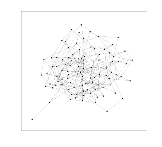
Figure 1: Communication topology used for discrete-time numerical study; $n=100,|\operatorname{\mathcal{E}}|=250$.

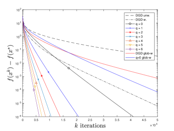
Figure 2: Comparison of weighted and unweighted DGD versus discrete distributed approx-Newton with various $q$ for solving ${\mathcal{P}}6$; $n=100,|\operatorname{\mathcal{E}}|=250$.

7.3 Continuous-Time Distributed Approx-Newton

We now study DANA-C for solving ${\mathcal{P}}1$ for a simple $3$ node network with two edges $\operatorname{\mathcal{E}}=\{\{1,2\},\{2,3\}\}$ for the sake of visualizing trajectories. The problem parameters are given by

$$f_{1}(x_{1})=\dfrac{1}{4}x_{1}^{2}+\dfrac{1}{2}x_{1},$$

$$f_{2}(x_{2})=\dfrac{3}{4}x_{2}^{2}+\dfrac{1}{2}x_{2},$$

$$f_{3}(x_{3})=2x_{3}^{2}+\dfrac{1}{2}x_{3},$$

$$\underline{x}=\begin{bmatrix}0.2&2.5&1.5\end{bmatrix}^{\top},\quad\overline{x}=\begin{bmatrix}1&6&4\end{bmatrix}^{\top},\quad d=6,$$

$$x^{0}=\begin{bmatrix}5&-1&2\end{bmatrix}^{\top},\quad z(0)=\boldsymbol{0}_{3},$$

$$\underline{\lambda}(0)=\begin{bmatrix}1.5&.5&0\end{bmatrix},\quad\overline{\lambda}(0)=\begin{bmatrix}0&2&1\end{bmatrix}$$

Note that $x^{0}$ is infeasible with respect to $\underline{x},\overline{x}$; all that we require is it satisfies Assumption 2 (feasible with respect to $d$). We plot the trajectories of the $3$-dimensional state projected onto the plane orthogonal to $\boldsymbol{1}_{3}$ under various $q$. Figure 3 shows this, with a zoomed look at the optimizer in Figure 4.

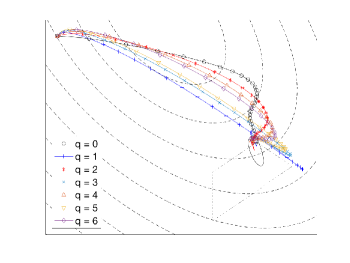
Figure 3: Three node case: projection of $x^{0}+Lz(t)\in\mathbb{R}^{3}$ onto the $2$-dimensional plane $\{x\;|\;\sum_{i}x_{i}=d\}$. Markers plotted for $t=0,0.2,0.4,\dots,5$ seconds. Dashed line ellipses indicate intersection of ellipsoid level sets with the plane; dotted lines indicate intersection of box constraints with the plane.

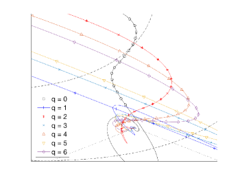
Figure 4: Three node case: trajectories zoomed closer to the optimizer. Markers plotted in $0.2s$ increments up to $t=5s$.

It is clear that choosing $q$ even versus $q$ odd has a qualitative effect on the shape of the trajectories, as noted in Section 6.3. Looking at Figure 3, it seems the trajectories are intially pulled toward the unconstrained optimizer (center of the level sets) with some bias due to $\lambda(0)\neq\boldsymbol{0}_{6}$. As $\lambda$ is given time to evolve, these trajectories are pulled back toward satisfying the box constraints indicated by the dotted quadrilateral, i.e. the intersection of the box constraints and the plane defined by $\{x\;|\;\sum_{i}x_{i}=d\}$.

For a quantitative comparison, we consider $n=40$ generators with $|\operatorname{\mathcal{E}}|=156$ communication links whose graph is given by Figure 5 and the following parameters.

$$f_{i}(x_{i})=\dfrac{1}{2}a_{i}x_{i}^{2}+b_{i}x_{i},\ a_{i}\in\mathcal{U}[0.5,3],\ b_{i}\in\mathcal{U}[-2,2],$$

$$\underline{x}_{i}\in\mathcal{U}[1.5,3],\quad\overline{x}_{i}\in\mathcal{U}[3,4.5],\quad i\in\{1,\dots,100\},$$

$$d=120,\ x^{0}=3*\boldsymbol{1}_{40},\ z(0)=\boldsymbol{0}_{40},\ \lambda(0)=\boldsymbol{0}_{80}.$$

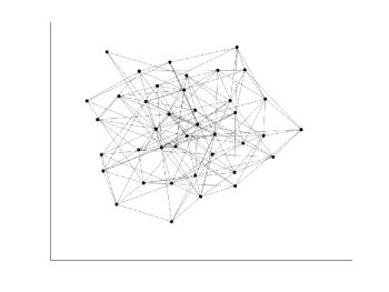
Figure 5: Communication graph for continuous-time numerical study: 40 nodes and 156 edges.

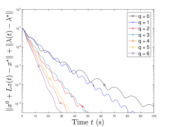
Figure 6: Error in the primal and dual state variables versus time for various $q$; $n=40,|\operatorname{\mathcal{E}}|=156$.

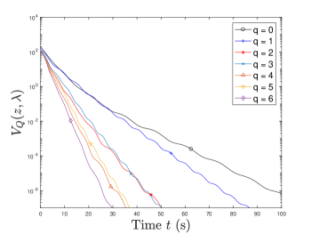
Figure 7: Value of the Lyapunov function $V_{Q}$ versus time for various $q$; $n=40,|\operatorname{\mathcal{E}}|=156$.

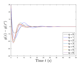
Figure 8: Value of the objective function versus time for various $q$; $n=40,|\operatorname{\mathcal{E}}|=156$.

Note from Figure 6 that convergence with respect to $\|x^{0}+Lz(t)-x^{\star}\|+\|\lambda(t)-\lambda^{\star}\|$ is not monotonic for some $q$. This is resolved in Figure 7 by examining $V_{Q}$ as defined by (29). We also note the phenomenon of faster convergence for even $q$ over odd $q+1$; the reason for this is related to the modes of $I_{n}-LHL$ and was discussed in Section 6.3. However, increasing $q$ on a whole lends itself to superior convergence compared to smaller $q$. As for the metric $g(z)-g(z^{\star})$ in Figure 8, note that these values become significantly negative before eventually stabilizing around zero. The reason for this is simple: in order for the $\mathscr{Z}_{q}$ dynamics (28) in $\lambda$ to “activate,” the primal variable must become infeasible with respect to the box constraints. In this sense, the stabilization to zero of the plots in Figure 8 represents the trajectories converging to feasible points of ${\mathcal{P}}2$.

7.4 Robust DANA Implementation

Lastly, we provide a simulation justification for relaxing Assumption 2 via the method described in Remark 1. Figure 9 plots the error in the primal and dual states over time of the modified “robust” method, which tends to approach zero for all observed values of $q$, and Figure 10 demonstrates that the violation of the equality constraint stablizes to zero very quickly. Noisy state perturbations are injected at $t=25,50,75$, and we observe a rapid re-approach to the plane satisfying the equality constraint. However, even though the algorithm presents a faster convergence than gradient methods, here do not observe as clear of a relationship between performance and increased $q$ as in previous settings. The investigation of the properties of this algorithm is left as future work.

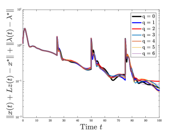
Figure 9: Error in the primal and dual states for a robust implementation of DANA; $n=20,|\operatorname{\mathcal{E}}|=40$. Initialization does not satisfy Assumption 2, and perturbations are injected at $t=25,50,75$.

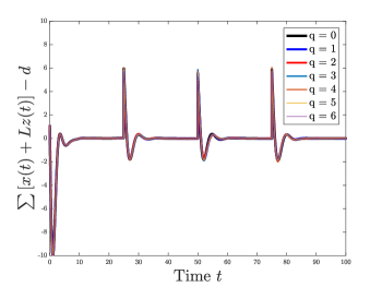
Figure 10: Violation of the resource constraint over time for robust DANA; $n=20,|\operatorname{\mathcal{E}}|=40$. Perturbations are injected at $t=25,50,75$.

8 Conclusion and Future Work

Motivated by economic dispatch problems and separable resource allocation problems in general, this work proposed a class of novel distributed approx-Newton algorithms. We first posed the topology design proplem and provided an effective method for designing communication weightings. The weight design we propose is more cognizant of the problem geometry, and it outperforms the current literature on network weight design even when applied to a gradient-like method. Our contribution on the second-order weight design approach is novel but is limited in scope to the given problem formulation. Distributed second-order methods are quite immature in the present literature, so an emphasis of future work is to generalize this weight design notion to a broader class of problems. Ongoing work also includes generalizing the cost functions for box-constrained settings and discretizing the continuous-time algorithm. In addition, we aim to develop distributed Newton-like methods suited to handle more general constraints and design for robustness under uncertain parameters or lossy communications. Another point of interest is to further study methods for solving bilinear problems and apply these to weight design within the Newton framework.

References

- [1] G. S. A. Wood, B. Wollenberg. Power Generation, Operation, and Control. John Wiley, 3 edition, 2012.
- [2] T. Anderson, C.-Y. Chang, and S. Martínez. Weight design of distributed approximate Newton algorithms for constrained optimization. In IEEE Conference on Control Technology and Applications, pages 632–637, Kohala Coast, Hawaii, USA, 2017.
- [3] S. Boyd and L. Vandenberghe. Convex Optimization. Cambridge University Press, 2004.
- [4] R. Carli and G. Notarstefano. Distributed partition-based optimization via dual decomposition. In IEEE Int. Conf. on Decision and Control, 2013.
- [5] R. Carli, G. Notarstefano, L. Schenato, and D. Varagnolo. Analysis of Newton-Raphson consensus for multi-agent convex optimization under asynchronous and lossy communications. In IEEE Int. Conf. on Decision and Control, pages 418–424, Osaka, Japan, 2015.
- [6] A. Cherukuri and J. Cortés. Initialization-free distributed coordination for economic dispatch under varying loads and generator commitment. Automatica, 74:183–193, 2016.
- [7] A. Cherukuri, E. Mallada, S. H. Low, and J. Cortés. The role of convexity in saddle-point dynamics: Lyapunov function and robustness. IEEE Transactions on Automatic Control, 63(8):2449–2464, 2018.
- [8] T. Doan and C. Beck. Distributed Lagrangian methods for network resource allocation. In IEEE Conference on Control Technology and Applications, 2017.
- [9] S. Friedberg, A. Insel, and L. Spence. Linear Algebra. Pearson, 4 edition, 2003.
- [10] S. Hassan-Moghaddam and M. Jovanovic. On the exponential convergence rate of proximal gradient flow algorithms. In IEEE Int. Conf. on Decision and Control, 2018.
- [11] A. Hassibi, J. How, and S. Boyd. A path-following method for solving BMI problems in control. In American Control Conference, pages 1385–1389, San Diego, CA, USA, 1999.
- [12] D. Jakovetic, J. Xavier, and J. Moura. Fast distributed gradient methods. IEEE Transactions on Automatic Control, 59(5):1131–1146, 2014.
- [13] H. Khalil. Nonlinear Systems. Prentice Hall, 2002.
- [14] E. Mallada, C. Zhao, and S. Low. Optimal load-side control for frequency regulation in smart grids. IEEE Transactions on Automatic Control, 62(12):6294–6309, 2017.
- [15] A. Mokhtari, Q. Ling, and A. Ribeiro. An approximate Newton method for distributed optimization. IEEE Transactions on Signal Processing, 65(1):146–161, 2017.
- [16] M. Mozaffaripour and R. Tafazolli. Suboptimal search algorithm in conjunction with polynomial-expanded linear multiuser detector for FDD WCDMA mobile uplink. IEEE Transactions on Vehicular Technology, 56(6):3600–3606, 2007.
- [17] Y. Nesterov. Introductory lectures on convex optimization: A basic course, volume 87. Springer Science & Business Media, 2013.
- [18] E. Ramírez-Llanos and S. Martínez. Distributed discrete-time optimization algorithms with application to resource allocation in epidemics control. Optimal Control, Applications and Methods, 2017. To appear. Available at the Wiley Online Library.
- [19] Y. Saad. Iterative methods for sparse linear systems. SIAM, 2003.
- [20] S. Y. Shafi, M. Arcak, and L. E. Ghaoui. Designing node and edge weights of a graph to meet Laplacian eigenvalue constraints. In Allerton Conf. on Communications, Control and Computing, pages 1016–1023, UIUC, Illinois, USA, 2010.
- [21] G. Stewart. Matrix Algorithms Volume 1: Basic Decompositions. SIAM, 1998.
- [22] J. VanAntwerp and R. Braatz. A tutorial on linear and bilinear matrix inequalities. Journal of Process Control, pages 363–385, 2000.
- [23] E. Wei, A. Ozdaglar, and A. Jadbabaie. A distributed Newton method for network utility maximization, I: Algorithm. IEEE Transactions on Automatic Control, 58(9):2162–2175, 2013.
- [24] E. Wei, A. Ozdaglar, and A. Jadbabaie. A distributed Newton method for network utility maximization, II: Convergence. IEEE Transactions on Automatic Control, 58(9):2176–2188, 2013.
- [25] L. Xiao and S. Boyd. Optimal scaling of a gradient method for distributed resource allocation. Journal of Optimization Theory & Applications, 129(3):469–488, 2006.
- [26] F. Zanella, D. Varagnolo, A. Cenedese, G. Pillonetto, and L. Schenato. Newton-Raphson consensus for distributed convex optimization. IEEE Transactions on Automatic Control, 61(4):994–1009, 2016.
- [27] F. Zhang. The Schur complement and its applications, volume 4. Springer, 2005.
- [28] M. Zhu and S. Martínez. Distributed Optimization-Based Control of Multi-Agent Networks in Complex Environments. Springer-Briefs in Electrical and Computer Engineering. 2015.