Multimodal Co-Training
for Selecting Good Examples from Webly Labeled Video^∗

Abstract.

We tackle the problem of learning concept classifiers from videos on the web without using manually labeled data. Although metadata attached to videos (e.g., video titles, descriptions) can be of help collecting training data for the target concept, the collected data is often very noisy. The main challenge is therefore how to select good examples from noisy training data. Previous approaches firstly learn easy examples that are unlikely to be noise and then gradually learn more complex examples. However, hard examples that are much different from easy ones are never learned. In this paper, we propose an approach called multimodal co-training (MMCo) for selecting good examples from noisy training data. MMCo jointly learns classifiers for multiple modalities that complement each other to select good examples. Since MMCo selects examples by consensus of multimodal classifiers, a hard example for one modality can still be used as a training example by exploiting the power of the other modalities. The algorithm is very simple and easily implemented but yields consistent and significant boosts in example selection and classification performance on the FCVID and YouTube8M benchmarks.

1. Introduction

Learning concept classifiers for videos is a fundamental task for automatic understanding of video and has many practical applications. Recent advances in deep neural networks enable very accurate classifiers to be learned by training on large-scale datasets with manually annotated labels (e.g., Kinetics dataset (Kay et al., 2017)). However, collecting such datasets involves huge amounts of human labor. Therefore, it is preferable to learn classifiers without using any manually labeled data.

One of the promising approaches to learning without labeled data is learning from web videos containing rich metadata (e.g., titles, descriptions, keywords). Such data are much easier to collect, and datasets consisting of millions of videos are available, e.g., YouTube8M (Abu-El-Haija et al., 2016), YFCC100M (Thomee et al., 2016). Although the training data for the target concept can be easily collected by using text-based matching between the concept name and metadata, the collected data are often noisy. The main challenge is therefore how to select good examples from noisy training data.

(a) Single modality

(b) Multiple modalities

Figure 1. In webly labeled learning, confident samples are selected as training examples from noisy data. (a) Previous approaches often miss hard examples that would potentially improve classifier performance. (b) The proposed approach can learn hard examples by exploiting the information of other modalities.

Liang et al. (Liang et al., 2016) proposed an approach to learning concept classifiers from web videos with noisy labels. The key idea is to learn easy examples first (Kumar et al., 2010; Bengio et al., 2009; Jiang et al., 2015). That is, easy examples that are very likely to be positive are learned first; then gradually more complex examples are learned. This idea is similar to self-training (Yarowsky, 1995) that is widely used in semi-supervised learning.

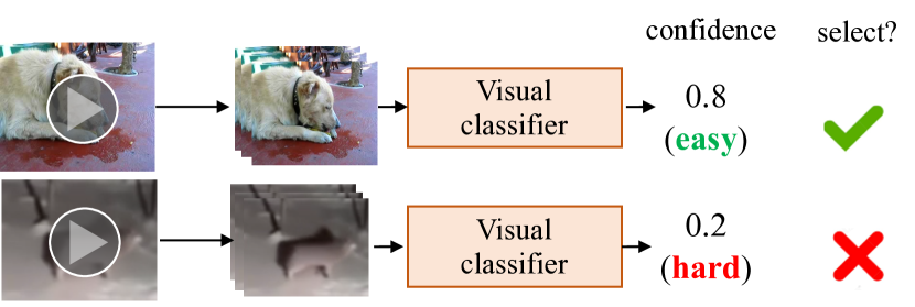
Although this approach can select correct examples that are easy, it sometimes misses hard correct examples. Consider hard samples that are much different from any easy sample; a classifier trained on only easy samples will never classify them as positive. In other research fields such as object detection, hard examples have been shown to be useful for improving a classifier. The basic approach of hard example mining is to select examples with high loss (Felzenszwalb et al., 2008; Girshick et al., 2014; Shrivastava et al., 2016; Schroff and Philbin, 2015). However, hard examples with high loss are likely to be noise in learning on noisy data. For example, in Fig. 1a, while the first easy sample can be used as a positive example, the second hard sample cannot be used because it is possible to be noise.

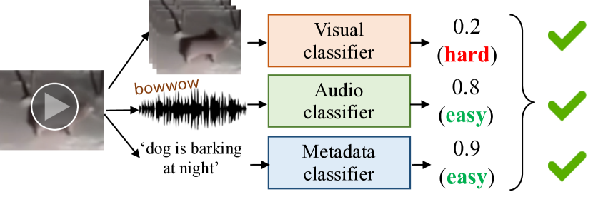
How can we select good examples that are hard and correct? Our key idea is to use information of multiple modalities. Figure 1 shows an example of learning a ‘dog’ classifier. The dog in the dark (Fig. 1b) is a hard example with only visual information because its appearance is much different from dogs in the light; such an example would not be selected in self-learning based approach. However, by using information of other modalities (e.g., the title ‘a dog is barking’ or sounds of dogs barking), we can confidently select it as a positive example.

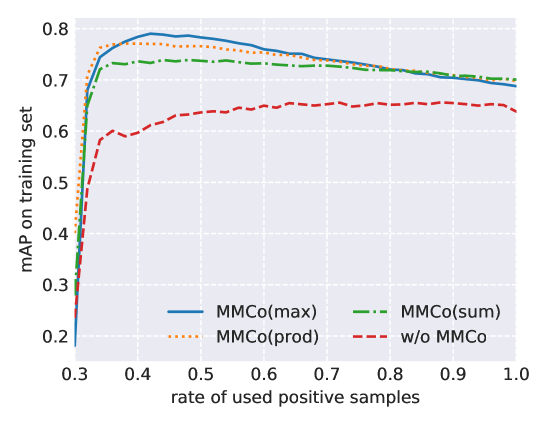
On the basis of this intuition, we propose an approach called multimodal co-training (MMCo) for selecting good examples by using multimodal knowledge. MMCo jointly learns the classifiers for multiple modalities and selects examples by voting of multiple classifiers (e.g., taking their max score). Therefore, a hard example for one modality can be used as a training example by exploiting the other modalities. The algorithm is very simple and easily implemented but significantly improve the performance of example selection from noisy training data; precision/recall is improved from 0.66/0.64 to 0.70/0.80 on FCVID benchmark.

In addition, we introduce an online learning algorithm for “webly” labeled learning problem (Liang et al., 2016). Although existing approaches (Liang et al., 2016, 2017) uses an alternating optimization that performs joint optimization of the model and the weights of the examples, it has trouble handling large-scale datasets consisting of millions of videos. Here, we extend the original webly labeled learning (WELL) (Liang et al., 2016) to an online setting by computing the sample weights online for each minibatch. This online WELL can handle a large-scale dataset without degrading accuracy. Online WELL can be extended to multiple classes easily and efficiently like other stochastic gradient descent(SGD)-based classifier learning methods.

2. Online Webly Labeled Learning

Our goal is to learn a concept detector from web videos without any manually annotated labels. Liang et al. (Liang et al., 2016) proposed Webly Labeled Learning (WELL) approach to this problem, where the classifier parameters and sample weights (selected examples) are alternately optimized. However, alternating optimization based on batch training is difficult to apply to a large-scale dataset consisting of millions of videos because all the training data should be processed in every update. We therefore decided to extend WELL to an online setting by selecting samples and computing their weight for each minibatch online. In this section, we first describe the problem of webly labeled learning and review WELL (Sec. 2.1). Then we describe online WELL (Sec. 2.2).

2.1. Background: Webly Labeled Learning

Problem formulation. Webly labeled learning was introduced in (Liang et al., 2016). In it, one considers the problem of learning a binary classifier $g$ for the concept from $N$ unlabeled web videos $\{(\mathbf{x}_{n},t_{n})\}_{n=1}^{N}$, where $\mathbf{x}_{n}$ is the feature of $n$th video, and $t$ is the metadata (text data) attached to it. The pseudo label of each example $y_{n}\in\{0,1\}$ is inferred by text-based matching between the concept name and the metadata of each video $t_{i}$; i.e., $y_{n}$=1 is assigned if the concept name $c$ appears in the metadata $t_{n}$, and $y_{n}$=0 if id does not appear. The confidence $v^{0}_{n}\in\mathbb{R}$ is obtained from the accuracy of matching; a high confidence value is assigned if $c$ frequently appears in $t_{n}$ ($v^{0}_{n}=1$ for negative-labeled samples). Consequently, the problem reduces to one of learning the classifier given the videos with pseudo labels and their confidences $\{(\mathbf{x}_{n},y_{n},v^{0}_{n})\}$.

The problem of webly labeled learning is related to semi-supervised (Chapelle, Olivier and Scholkopf, Bernhard and Zien, 2009) and noisy-labeled learning (Frénay and Verleysen, 2014). In noisy-labeled learning, a classifier is learned using samples with noisy (corrupted) labels ($\mathbf{x}_{n}$, $y_{n}$). While all samples should be treated equally in noisy-labeled learning, in webly labeled learning, the label confidence $v^{0}_{n}$ of each sample can be obtained from metadata as prior knowledge. In semi-supervised learning, a classifier is learned using both labeled and unlabeled samples. While labeled samples are completely trusted in semi-supervised learning, in webly labeled learning, samples with high confidence labels are not always positive.

Model. We here describe the Webly Labeled Learning (WELL) model (Liang et al., 2016) that was proposed to solve the problem formulated above. WELL is based on the self-paced curriculum learning theory proposed in (Jiang et al., 2015). The model parameters $\mathbf{w}$ (e.g., linear classifier weights) and the latent weight variable $\mathbf{v}=[v_{n},...,v_{N}]^{T}$ are jointly learned by alternating optimization. The objective function is defined as

(1) $$\min_{\mathbf{w},\mathbf{v}}E(\mathbf{w},\mathbf{v};\lambda)=\sum_{n=1}^{N}v_{n}L(y_{n},g(\mathbf{x}_{n},\mathbf{w}))+f(\mathbf{v};\lambda),$$

where $g$ is the classifier, $L$ is the loss function, and $\mathbf{v}=[v_{1},v_{2},...,v_{N}]^{T}$ denote the latent weight variables that reflect label confidences. Examples with larger weights tend to be learned with high priority. $f$ is a self-paced regularizer (Kumar et al., 2010) that controls the learning process so that easy samples with small losses tend to be selected earlier. For example, the linear regularizer proposed in (Jiang et al., 2015) is

(2) $$f(\mathbf{v};\lambda)=\frac{1}{2}\lambda\sum_{n=1}^{N}(v_{n}^{2}-2v_{n})$$

where $\lambda$ controls the learning pace; i.e., $\lambda$ is gradually increased to increase the number of samples used. With a fixed $\mathbf{w}$, the weight variable can be optimized in a closed form as

(3) $$v_{n}=\left\{\begin{aligned} 1-\tfrac{l_{n}}{\lambda}\qquad&l_{n}<\lambda,\\ 0\qquad&l_{n}\geq\lambda,\end{aligned}\right.$$

where $l_{n}$ is the loss for the $n$th sample. Therefore, examples with losses smaller than $\lambda$ are used for training.

$\mathbf{v}$ is initialized by the pseudo label’s confidence $\mathbf{v}^{0}$ computed by word matching between the concept name and metadata, which corresponds to the intuition of curriculum learning (Bengio et al., 2009) that determines the learning sequence from external prior knowledge. WELL determines the learning sequence by using both prior knowledge in the manner of curriculum learning and the model in the manner of self-paced learning. In this way, WELL can learn from easy examples as well as from more complex ones.

Below, we summarize the implementation of WELL.

1. Initialize the sample weights $\mathbf{v}$ from the label confidence $\mathbf{v}^{0}$.

2. Update the model $\mathbf{w}$ with fixed sample weights $\mathbf{v}$.

3. Compute the losses of all examples by using the updated model.

4. Compute the weights $\mathbf{v}$ of all examples by using Eq. 3.

5. Increase age $\lambda$.   Repeat (2)–(5) until convergence.

2.2. Online Webly Labeled Learning

Although WELL learns the classifier by alternating minimization, it is not appropriate for the training on a large-scale dataset. In alternating optimization, all training samples are used to optimize the model $\mathbf{w}$ in every iteration, wherein the sample weights $\mathbf{v}$ are fixed when optimizing the model. If the training data is very large (e.g., millions of samples), it takes a very long time to complete one iteration, which makes convergence very slow. In addition, it is generally infeasible to put whole dataset in memory. Hence, we decided to extend the webly labeled learning model in (Liang et al., 2016) to the online learning based on stochastic gradient decent (SGD).

The main problem is how to select optimal samples and compute their weights in a minibatch. If the sample weights $\mathbf{v}$ are given, the model can be stochastically optimized over the minibatch in the manner of SGD. Although alternating optimization generally requires all samples in order to optimize each variable, in the binary scheme of WELL, the weight $v_{n}$ can be computed using only the loss of the sample $l_{n}$ and the model age $\lambda$ using Eq. 3. Therefore, we can compute the sample weight $v_{n}$ online after computing the loss of each sample $l_{n}$, where the model is updated with the weighted loss $v_{n}l_{n}$. The age is determined by the scheduler described below.

More specifically, the online webly labeled learning algorithm is as follows.

1. Initialize model $\mathbf{w}$ and age $\lambda$.

2. Randomly sample a minibatch with $N_{m}$ examples.

3. Compute the losses $l_{1},..,l_{N_{m}}$ using the model $\mathbf{w}$. Cross entropy loss is used in this study.

4. Compute the weights $v_{1},..,v_{N_{m}}$ of the samples in the minibatch with Eq. 3 and the computed losses (the confidences of the pseudo labels $\mathbf{v}^{0}$ are used in the first few iterations.)

5. Update $\mathbf{w}$ by using the weighted losses, i.e., $\sum_{i=1}^{N_{m}}v_{i}l_{i}$

6. Increase the age $\lambda$ based on the age scheduler described below.

Repeat (2)–(5) until convergence.

We should note that the training cost of online WELL is less than that of WELL. WELL needs to compute the loss twice in each iteration in order to update the weights $\mathbf{w}$ and the model $\mathbf{v}$. On the other hand, we have to compute the loss only once; sample weights $\mathbf{w}$ are computed using the loss, and the model $\mathbf{v}$ is updated using the weighted loss.

Age scheduling. Model age $\lambda$ is an important parameter that determines which samples to select as examples. Manually determining the age schedule (initial value, early stopping value, etc.) is hard; in practice, the age is controlled in accordance with the rate of used samples in the positive pool $p$ (e.g., 30% positive samples ($p$=0.3) are first used, and $\lambda$ is gradually increased until 60% positive samples ($p$=0.6) are used), which can be specified more intuitively. The age $\lambda$ is computed from $p$ by sorting all positive samples, where the loss at the $100p$th percentile is $\lambda$. However, in online learning, not all of the training samples are available for the updates, the age cannot be computed from $p$.

To control $\lambda$ in online learning, we introduce a FIFO queue that stores the losses of the previous iterations. We can compute $\lambda$ from $p$ by regarding the samples in the queue as a whole training set. There are two approximations here. First, the samples in the queue approximate the whole set of training samples; the size of the queue should be large enough to hold enough samples. Second, the losses in the queue are computed from the previous model; they are different from the loss computed by the current model. The size of the queue should not be too large because of this. Although there is a trade-off between these two approximations, the same performance as in batch training can be achieved by selecting an appropriate queue size.

Multiple classes. Online WELL is easily extended to multiple classes like other multilabel classification models learned by SGD. Given a dataset $\{(\mathbf{x}_{n},\mathbf{y}_{n})\}_{n=1}^{N}$, the goal is to learn a multilabel classifier that outputs the confidence of $C$ classes, where $\mathbf{y}_{n}=[y_{n,1},...,y_{n,C}]^{T}\in\{0,1\}^{C}$ are labels for $C$ classes. Note that we do not assume that the classes are mutually exclusive; therefore, the samples can be positive for multiple classes. For each iteration, the age $\lambda_{C}$ is determined for each class independently following the age scheduling described above, whereby the weights of the samples $\mathbf{V}\in\mathbb{R}^{N\times C}$ are computed for every class. The loss in a minibatch can be computed as

(4) $$\sum_{n=1}^{N}\sum_{c=1}^{C}\mathbf{V}_{n,c}L(\mathbf{y}_{n,c},g(\mathbf{x}_{n},\mathbf{w},c)),$$

where $g(\cdot,\cdot,c)$ is the prediction for the $c$th class. By sharing the computation, this algorithm enables multiple classifiers to be learned much more efficiently than learning each classifier independently, especially computationally heavy classifiers like deep neural networks.

Figure 2. Overview of proposed approach using MMCo. Classifiers of multiple modalities are jointly learned. While the loss is computed for each classifier independently, weights of examples are determined by voting of multiple classifiers.

3. Multimodal Co-Training

In webly labeled learning, easy examples with small losses are preferentially used as training data. Correct but hard examples that would potentially improve performance are never learned. As a solution to this problem, we propose multimodal co-training (MMCo) as a way to use multimodal information in web videos (e.g., visual, audio, and metadata), which enables us to exploit hard examples. For example, a sample with a small loss in the audio modality but large loss in the visual modality could be a hard (but correct) sample from the visual perspective (a dog at night maybe). MMCo can utilize such samples by selecting examples on the basis of the consensus of the classifiers of individual modalities. Hard examples for one modality can still be used as a training example by exploiting the power of the other modalities. In this way, the classifiers of individual modalities mutually enhance each other. The underlying motivation of our approach is very close to that of co-training in semi-supervised learning (Blum and Mitchell, 1998), which is discussed in Sec. 3.3.

3.1. Model

We jointly learn multiple modality classifiers. Given a dataset consisting of multiple modality features and pseudo labels $\{(\mathbf{x}_{n}^{1},...,\mathbf{x}_{n}^{M}),y_{n}\}_{n=1}^{N}$, the goal is to learn classifier parameters for multiple modalities $(\mathbf{w}^{1},...,\mathbf{w}^{M})$, where $M$ is the number of modalities. The classifier of each modality $g^{m}(\mathbf{x}_{n}^{m},\mathbf{w}^{m})$ is learned with the loss computed in the same way as single modality (Eq. 4). The only difference is the way of computing the weight variable $v_{n}$. $v_{n}$ reflects the label confidence, and thus does not depend on modality $m$, i.e., the same weight is used across all modalities. Therefore, we determine the selected samples and their weights by the consensus of classifiers of all modalities.

Sample selection. We here describe how to select examples in MMCo, i.e., how to compute sample weights $v_{n}$. In a previous approach, the weight is computed from the loss using Eq. 3, in which the loss is computed using the cross entropy between the confidence $g(\mathbf{x},\mathbf{w})$ and label $y$. The confidence is computed by the voting of multiple classifiers. Specifically, the sample weight $v_{n}$ is calculated as follows:

(5) $$v_{n}=\mathrm{max}(0,1-\frac{L(s_{n},y_{n})}{\lambda}),$$

where the confidence $s_{n}$ of the sample is

(6) $$s_{n}=h(g^{1}(\mathbf{x}_{n}^{1},\mathbf{w}^{1}),...,g^{M}(\mathbf{x}_{n}^{M},\mathbf{w}^{M})),$$

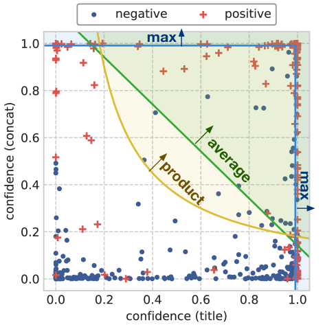
where $h$ is the voting function that takes the input of multiple classifier confidences $\{g^{m}(\mathbf{x}_{n}^{m},\mathbf{w}^{m})\}_{m=1}^{M}$. We introduce three types of simple voting scheme, namely, max ($\max_{m}g^{m}(\mathbf{x}_{n}^{m},\mathbf{w}^{m})$), average ($\frac{1}{M}\sum_{m}g^{m}(\mathbf{x}_{n}^{m},\mathbf{w}^{m})$), and product ($\prod_{m}g^{m}(\mathbf{x}_{n}^{m},\mathbf{w}^{m})$). This enable us to use hard examples of each classifier. For example, with max voting, if $g^{1}(\mathbf{x}_{n}^{1},\mathbf{w}^{1})$ is small and $g^{2}(\mathbf{x}_{n}^{2},\mathbf{w}^{2})$ is large, a large weight is assigned to this sample although it is a hard example for $g^{2}$. Our discussion for a single class can be extended to multiple classes in the same manner of Sec. 2.2.

3.2. System Design

The modalities used in this study are RGB, motion, audio, and metadata (see Sec. 4.1 for the details of the features). In addition, the concatenated features of all modalities extracted from video (RGB, motion, and audio) are used as another modality, which we call concat feature. In training, the classifiers of all modalities are used and mutually enhanced by our co-training approach. In testing, only the classifier of the concat feature is used; metadata information is not used, because we assume that metadata is not available for the test videos (It is also possible to use a metadata classifier for classifying the videos with metadata). We found that using the classifier for concatenated features worked better than using classifiers for multiple modalities.

The important point here is that a modality that cannot be used in testing can be used for training. For example, we can train the classifiers for the metadata modalities even if metadata is not available in the testing; a video-content classifier can be improved by co-training with a metadata classifier. On the other hand, the original WELL is based on self-paced learning, and thus, it cannot fully exploit metadata modality information (it can only be used to extract pseudo labels).

Although we can use any type of classifier for each modality, from the aspect of large-scale retrieval, it is better to use a linear classifier in testing than a more complex classifier such as a deep neural network. Large-scale retrieval is one of the main applications of video concept classifier learning. To retrieve from large amounts of video, the classifier should be scalable. A linear classifier is easy to scale for a large database, whereas a deep neural network is difficult to scale. Although the scalable classifier should be used in testing, any type of classifier can be used for another modality in training. Therefore, our approach can exploit the power of a strong classifier (e.g., a deep neural networks) to select good examples from noisy training data, while previous self-paced learning-based approaches select examples using only the testing classifier.

3.3. Relationship with prior work

Self-training, co-training: Self-training (Yarowsky, 1995) and co-training (Blum and Mitchell, 1998) are commonly used techniques in semi-supervised learning. In self-training, a classifier is first learned with a small amount of labeled data; then, it is applied to unlabeled data, wherein the most confident samples are added as new training examples. On the other hand, co-training iteratively train classifiers on two different views, where new training examples of each classifier are determined by the prediction of the other classifier. While the idea of WELL (Liang et al., 2016) is based on self-training that selects examples for the classifier by using its own predictions, MMCo incorporates the idea of co-training; examples for each classifier are selected on the basis of the predictions of other classifiers as well as its own predictions. Unlike co-training in semi-supervised learning, MMCo does not involve an iterative process, so it can easily handle more than two classifiers.

Multimodal ensemble learning: Our approach selects examples on the basis of the consensus of classifiers for multimodal features, which is the same idea as ensemble learning (Dietterich, 2002) that makes predictions by combining multiple classifiers. It is known that an effective ensemble learning system should consist of diverse classifiers (Sun, 2010; Sun and Zhang, 2007), and several studies have investigated the use of complementary multimodal information in videos for ensemble learning (Hsu, 2004; Chang et al., 2007; Fan et al., 2007). While ensemble learning is generally used to improve prediction accuracy, our approach uses an ensemble of multimodal classifiers to select good examples from noisy training data. Although we investigated only simple voting of classifiers, other ensemble learning techniques (Freund and Schapire, 1997; Wolpert, 1992; Breiman, 1996) could be integrated into our approach.

Learning from search engine results: While we tackle webly labeled learning (Liang et al., 2016, 2017) that learns from web videos with weak annotations, there is another type of webly supervised classifier learning which directly uses results returned by search engines (Fergus et al., 2005; Chen and Gupta, 2015; Yeung et al., 2017; Chatfield and Zisserman, 2012; Chatfield et al., 2015). This type typically uses a search engine (e.g., YouTube) to search by concept name and learns a classifier by using the retrieved results as positive samples. Since the challenge is similar to our problem, i.e., how to handle noise in the search results, our approach could be applied for this problem by using the search results as positive-labeled noisy training data and the search rank to compute the initial label confidence (i.e., top-ranked videos are likely to be positive).

(a)

(b)

(c)

Figure 3. Sample selection quality on FCVID training set. (a) precision/recall curve. (b) transition of recall (blue) and precision (orange). (c) transition of mAP on training set

4. Experiments

4.1. Experimental Settings

Datasets. The main evaluation used Fudan-columbia Video Dataset (FCVID) (Jiang et al., 2018) as the main evaluation. FCVID contains 91,223 videos from YouTube, totaling 4232 hours of videos. The dataset contains ground truth annotations at the video level for 239 categories including activities, objects, scenes, etc. We used the standard partitioning of the training/test set provided by (Jiang et al., 2018). We did not use the manual labels in training. Instead, we inferred pseudo labels from the metadata (title and description) in the same manner as (Liang et al., 2016). In addition, we used the YouTube8M dataset (Abu-El-Haija et al., 2016) in the larger scale evaluation.

Features. We first extracted features from videos and used them as classifier inputs. In the evaluation of FCVID, we used the following features for each modality. RGB: Frame-level features were first extracted from keyframes by VGG (Simonyan and Zisserman, 2015) trained on ILSVRC, and a video-level feature was then computed by average pooling; these were the same features used in (Liang et al., 2016). Motion: P3D Resnet features were extracted in the manner described in (Qiu et al., 2017). We used the model trained on the Kinetics dataset (Kay et al., 2017), which is provided by (Hara et al., 2018). Audio: We extracted 128-dimensional VGGish features produced from a VGG-like audio classification model (Hershey et al., 2017). We used the model trained on the YouTube8M dataset (Abu-El-Haija et al., 2016) provided by Google. Metadata: TextCNN features were extracted from the title of the YouTube video following (Wang et al., 2017). We used the model provided by (Wang et al., 2017), which was trained on the YouTube8M dataset. Concat: The features of RGB, Motion, and Audio are concatenated.

In the YouTube8M evaluation, we used the officially provided RGB and audio features (1024-dimensional GoogLeNet (Szegedy et al., 2015) feature and 128-dimensional VGGish feature). For metadata, we used the same features as FCVID evaluation.

Classifiers. We used a linear classifier for all modalities except audio. A multi-layer perceptron with one hidden layer (4096 units) was used for audio feature classifier.

Training. The model age $\lambda$ was determined from the rate of used positive examples $p$; $p$ was initialized as 0.3, which is increased by 0.05 every five epochs and early stopped at $p$=0.6. The training labels (i.e., pseudo labels $y_{n}$ and their confidences $v_{n}^{0}$) were obtained by word hard matching in the same way as (Liang et al., 2016). Adam optimizer (Kingma and Ba, 2015) was used to update the model with initial learning rate $10^{-3}$.

	Modality
Method	Training	Testing	Voting	mAP
BatchTrain (Liang et al., 2016)	VGG	VGG	-	0.469
SPL (Kumar et al., 2010)	VGG	VGG	-	0.414
GoogleHNM (Toderici and Natsev, 2015)	VGG	VGG	-	0.472
BabyLearning (Liang et al., 2015)	VGG	VGG	-	0.496
WELL (Liang et al., 2016)	VGG	VGG	-	0.565
WELL-MM (Liang et al., 2017)	VGG+MM	VGG	-	0.615
WELL*	Concat	Concat	-	0.619
Online WELL	Concat	Concat	-	0.621
Online WELL w/ MMCo	VGG + P3D +Audio +TextCNN +Concat	Concat	Max	0.663
			Sum	0.622
			Product	0.630

Table 1. Performance comparison on FCVID test set

4.2. Comparison with Baselines

We compared final classification performances of the classifiers trained on the web videos on FCVID. The main objective of this comparison was to determine whether online WELL achieves comparable performance to the conventional WELL based on alternating optimization and whether MMCo improves performance. To this end, we reproduced WELL with the same features and parameters and compared it with the online WELL with and without MMCo. We used concat features in our reproduction of WELL for a fair comparison.

Table 1 shows the results. Online WELL achieves comparable performance to WELL using the same features. MMCo with max voting improves mAP by 4.2 points relative to WELL without MMCo. It also significantly outperforms the other baselines (Kumar et al., 2010; Toderici and Natsev, 2015; Liang et al., 2015). Although the different features are used for the comparison, our approach improves even on WELL that is much better than the others with the same VGG features. In addition, WELL-MM (Liang et al., 2017) and MMCo are complementary extensions of WELL. WELL-MM infers pseudo labels and their confidences using multimodal knowledge instead of word matching, which can easily be incorporated into our approach simply by changing pseudo labels.

4.3. Evaluation of Example Selection

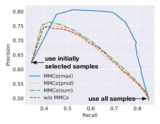
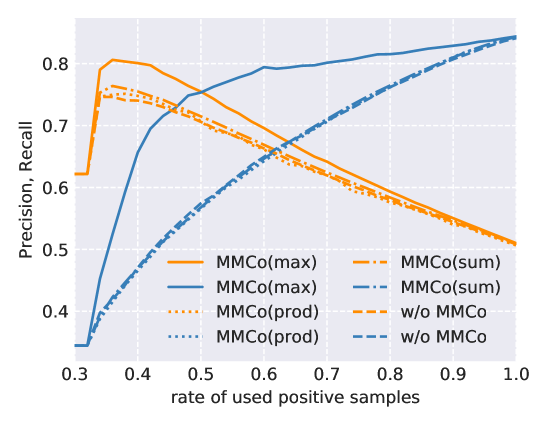
To show that MMCo selects good examples from noisy training data, we evaluated the performance of example selection. In webly labeled learning, the samples with the loss smaller than the age were used as positive samples as described in Eq.3; we measured the quality of selected positive samples by recall, precision, and AP. Recall and precision were computed as the number of selected positive samples divided by the total number of positive samples and the total number of selected samples, respectively, and AP was computed by the ranking of losses for all positive samples. We used online WELL and compared with and without MMCo. Voting schemes were also compared. The baseline (w/o MMCo) computed the sample weights using one classifier for concat features while the proposed approach (w/ MMCo) computed weights by the voting of classifiers of all five modalities.

Figure 3 shows the precision/recall curve and performance during the training. The proposed MMCo with max voting (MMCo (max)) performed significantly better than the baseline. When the rate of used samples was 0.6 (in Fig. 3b), the precision/recall of MMCo (max) was 0.70/0.80, which is much better than the results of the baseline without MMCo (0.66/0.64) and the results using all samples with pseudo labels (0.49/0.85). These results clearly demonstrate the effectiveness of MMCo. The experiments in Sec. 5.1 provide a more detailed analysis of example selection and discuss why max voting performs the best.

4.4. Large-Scale Evaluation on YouTube-8M

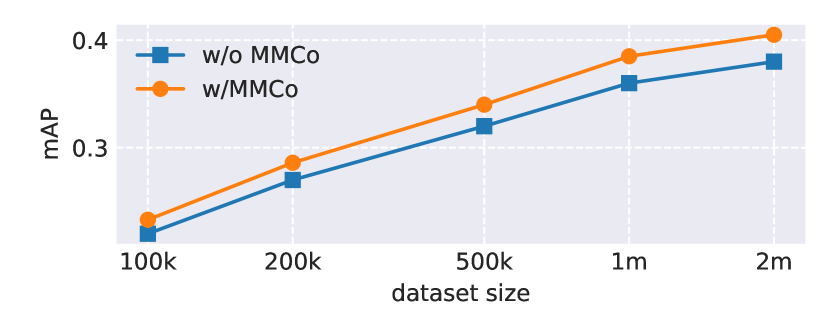
The YouTube-8M dataset contains millions of videos; it is too big to be handled by the conventional approach based on alternating minimization. We conducted an evaluation on the YouTube-8M dataset to determine whether the performance of online WELL gets better on larger-scale datasets. We varied the size of the dataset by randomly selecting samples. We evaluated mAP for the 500 most frequently appearing classes from all 4716 classes, because samples from many classes in YouTube8M rarely appear when the size of the dataset is small. Figure 4 shows the performance of our approach with and without MMCo (max voting) for different subset sizes. mAP increases along with the size of the noisy training data up to two million samples. MMCo consistently improves mAP for any dataset size (about a 5% relative improvement). The results show that online WELL has the potential to increase its accuracy, because it can handle an unlimited number of videos and noisy training data is easy to collect.

Figure 4. Dataset size vs test mAP on YouTube8M.

5. Detailed Analysis

We conducted a more detailed analysis to better understand the behavior of MMCo. We used max voting unless otherwise specified.

	mAP			Recall
	easy	normal	hard	easy	normal	hard
w/ MMCo	0.655	0.642	0.506	0.823	0.709	0.579
w/o MMCo	0.700	0.592	0.256	0.857	0.648	0.299

Table 2. Sample selection performance in terms of the difficulty (easiness) of samples. The same number of positive-labeled samples is used for both conditions ($p$=0.6).

(a) Without MMCo

(b) With MMCo

Figure 5. Easiness distribution of selected examples

(a)

(b)

Figure 6. Selected samples of ‘cello performance’ class in FCVID. (a) Regions of selected samples are shaded: max (blue), average (green), and product (yellow). (b) Examples that are hard for only one modality. The upper and lower row shows examples with high confidence for metadata and concat modality, respectively (upper left and lower right samples in (a), respectively).

5.1. Are hard samples actually selected?

The motivation of MMCo is to select hard positive examples that cannot be selected by the previous approach. We performed three analyses to validate MMCo really select hard samples.

Performance by difficulty: We evaluated the performance of example selection in terms of the difficulty, or easiness, of the samples. The objective of this experiment was to show that the samples that cannot be detected by initial classifiers can be rescued by the proposed approach. Therefore, we define easiness as a classification score using the classifier trained on the top 30% of samples with a high pseudo label’s confidence $v^{0}_{n}$. We divided the positive samples in the training data into three sets in terms of by easiness, i.e., easy, normal, and hard; the samples were sorted by easiness score for each class, where the 30, 40, and 30th percentiles of samples are selected as easy, normal, and hard, respectively. Table 2 shows the example selection performance of each difficulty set. MMCo significantly improves the performance of hard samples in terms of both mAP (from 0.256 to 0.506) and recall (0.299 to 0.579), while there is no big difference for easy and normal samples.

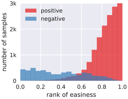
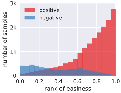
Distribution of difficulties of selected examples: We performed a more detailed analysis of selected examples. We compare the distribution of easiness (defined above) with and without MMCo. Figures 5a and 5b shows the results with and without MMCo, respectively, where the x-axis shows the rank of easiness scores among all positive-labeled examples, which is normalized to [0,1]. The MMCo selected positive hard examples with the scores in the range [0,0.5], while the method without MMCo did not select them often. Note that there is not a big difference in the number of selected negative examples (i.e., false positive samples), which shows MMCo selects only true positive examples from hard samples.

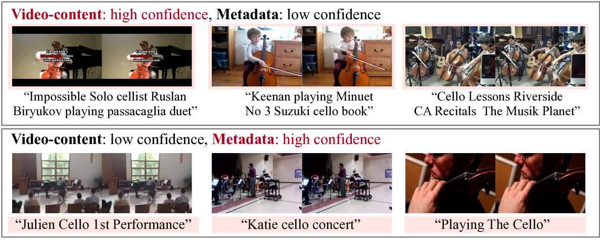
Qualitative analysis: We qualitatively analyzed the selected examples. We picked ‘cello performance’ class of FCVID and watched the detail of the selected examples. We again used the classification scores of the classifier trained on top 30% examples, i.e., the same condition under which samples were first selected by MMCo. Figure 6a shows the metadata and concat classifier scores of positive labeled training samples, where true and false positive examples are depicted in red and blue. The selected samples of each voting scheme is shaded in color (when using only metadata and concat scores). The results suggest why max voting performed better than other voting schemes. We can see that the samples with high confidence for one modality are likely to be positive, while the samples with low confidence are not always negative. For example, there are some positive samples with zero confidence for one modality (lower right and upper left in the figure), which are hard samples for the modality but selected by using max voting. Figure 6b shows examples of these hard positives. Metadata classifier assigns high scores to simple titles (second row) and low scores to long titles that are difficult to parse (first row). By learning with such hard examples, metadata classifiers learns the key words or phrases of ‘cello performance’ such as ‘cellist’, ‘playing’, and ‘cello lessons’. Video-content classifier (concat) is also improved by learning with examples that are hard from the visual perspective (second row).

	Modality in training					Sample selection			Test performance
Method	RGB	Motion	Audio	Concat	Metadata	mAP	precision	recall	mAP	Prec@10	Prec@100
Unimodal	✓					0.538	0.603	0.632	0.612	0.835	0.752
		✓				0.539	0.601	0.632	0.605	0.841	0.755
			✓			0.328	0.512	0.592	0.594	0.788	0.658
				✓		0.640	0.656	0.645	0.621	0.845	0.766
					✓	0.676	0.632	0.702	0.639	0.868	0.777
Multimodal	✓	✓	✓			0.663	0.621	0.714	0.626	0.844	0.769
				✓	✓	0.781	0.693	0.801	0.660	0.880	0.791
	✓				✓	0.749	0.652	0.753	0.646	0.857	0.765
	✓	✓			✓	0.774	0.682	0.780	0.661	0.860	0.793
	✓	✓	✓		✓	0.772	0.688	0.783	0.662	0.873	0.784
	✓	✓	✓	✓	✓	0.770	0.694	0.803	0.663	0.862	0.781

Table 3. Combinations of modalities used in training. The testing classifier is the same (concat) for all settings.

5.2. Which modalities improve performance?

To investigate which modalities improve performance, we tested with varied combination of modalities. Since our main interest is the improvement in example selection performance, we only changed training modalities that are used to compute scores for example selection. We used the concat feature in the testing in all experiments. Table 3 shows the results for various modality combinations; rows 1–5 are for only a single modality, while rows 6–11 are for multiple modalities. The results provide several important findings. 1) The results using both video-content and metadata modality (rows 7–11) are much better than those using only either type of features (rows 1–6). This suggests that using modalities with complementary information is more important than using just multiple modalities. 2) Among the video-content related features, P3D contributed significantly to performance improvements, while audio did not contribute very much (row 8–10). 3) The results for Concat + Metadata (row 7) are comparable to those of using more than two classifiers, which is a practically reasonable choice in terms of the trade-off between the training cost and test accuracy.

Figure 7. Noise level vs test mAP on FCVID.

Figure 8. Top retrievals on FCVID dataset. Retrievals were performed by using the classifier trained with the webly label, where the results are sorted by classification score and marked as negative (red) or positive (green).

5.3. Noise robustness

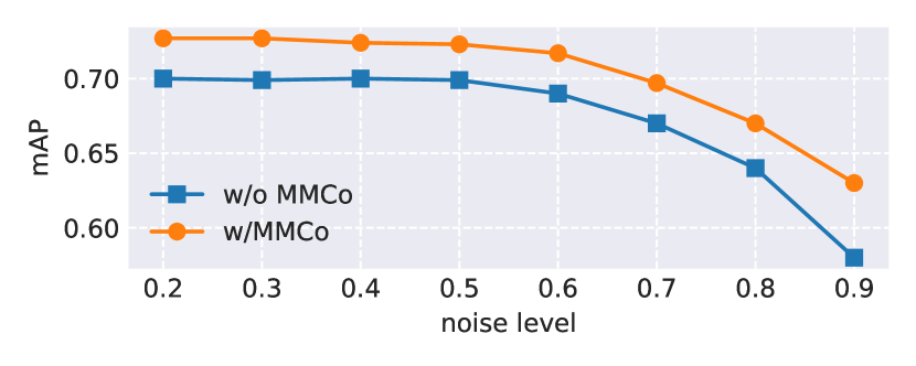
We evaluated the robustness of our approach to noise by manually controlling the amount of noise in the training data. Since the training data of our task is noisy, there are true and false positives among the positive-labeled samples. We varied the noise level $n_{FP}/(n_{TP}+n_{FP})$ in the range of 0.2 to 0.9, where $n_{TP}$ and $n_{FP}$ are the number of true and false positives, respectively. We fixed the true positive samples and randomly selected false positive samples as artificial noisy samples. Figure 7 compares the performances of our approach with and without MMCo on FCVID for different noise levels. Our approach (w/ MMCo) was consistently better than the baseline (w/o MMCo) with any amount of noise. It scored 0.63 in mAP at a noise level of 0.9, which demonstrates that it can work on a very noisy dataset.

5.4. Qualitative examples

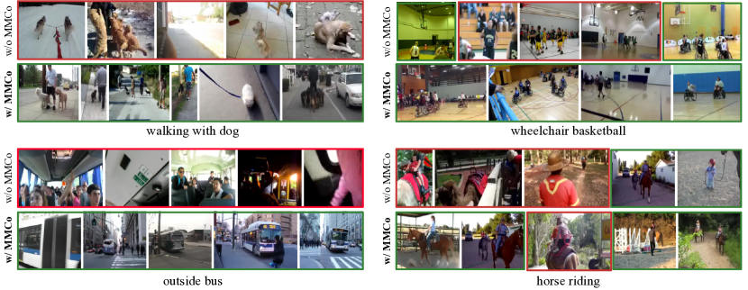
Figure 8 shows the top retrieval results on FCVID by using the classifiers trained by webly labeled learning. The results with and without MMCo are compared to qualitatively demonstrate the effectiveness of our approach. While the approach without MMCo detects many false positives of very similar concept, the approach with MMCo rejects such false positives by effectively using the metadata information in training. Since our trained classifier is a simple linear classifier, this retrievals can be performed in less than one second from 48,435 videos. It is also easy to extend million or billion-scale retrievals by using the techniques of approximate nearest neighbor search (Jégou et al., 2011).

6. Conclusion

We presented a multimodal co-training (MMCo) algorithm, a simple and effective method for learning concept classifier from videos on the web. MMCo can selects good examples from noisy training data by jointly learning classifiers of multiple modalities and selecting examples based on their consensus. We conducted an extensive experimental analysis to demonstrate the effectiveness of MMCo, which demonstrated better example selection and consistent improvements in webly labeled learning on FCVID dataset over baseline methods. Our detailed analysis from multiple aspects further examined the behavior of MMCo and provided several useful insights about how to exploit multimodal information effectively in webly supervised learning.

References

- (1)
- Abu-El-Haija et al. (2016) Sami Abu-El-Haija, Nisarg Kothari, Joonseok Lee, Paul Natsev, George Toderici, Balakrishnan Varadarajan, and Sudheendra Vijayanarasimhan. 2016. YouTube-8M: A Large-Scale Video Classification Benchmark. In arXiv preprint.
- Bengio et al. (2009) Yoshua Bengio, Jérôme Louradour, Ronan Collobert, and Jason Weston. 2009. Curriculum learning. In ICML.
- Blum and Mitchell (1998) Avrim Blum and Tom Mitchell. 1998. Combining labeled and unlabeled data with co-training. In COLT.
- Breiman (1996) Leo Breiman. 1996. Bagging predictors. Machine Learning 24, 2 (1996), 123–140.
- Chang et al. (2007) Shih-Fu Chang, Dan Ellis, Wei Jiang, Keansub Lee, Akira Yanagawa, Alexander C. Loui, and Jiebo Luo. 2007. Large-scale multimodal semantic concept detection for consumer video. In Proceedings of the international workshop on Workshop on multimedia information retrieval - MIR ’07.
- Chapelle, Olivier and Scholkopf, Bernhard and Zien (2009) Alexander Chapelle, Olivier and Scholkopf, Bernhard and Zien. 2009. Semi-Supervised Learning. IEEE Transactions on Neural Networks 20, 3 (2009), 542–542.
- Chatfield et al. (2015) Ken Chatfield, Relja Arandjelovi, Andrew Zisserman, Relja Arandjelović, Omkar Parkhi, and Andrew Zisserman. 2015. On-the-fly learning for visual search of large-scale image and video datasets. International Journal of Multimedia Information Retrieval 4, 2 (2015), 75–93.
- Chatfield and Zisserman (2012) Ken Chatfield and Andrew Zisserman. 2012. VISOR : towards on-the-fly large scale object category retrieval. In ACCV.
- Chen and Gupta (2015) Xinlei Chen and Abhinav Gupta. 2015. Webly supervised learning of convolutional networks. In ICCV.
- Dietterich (2002) Thomas G. Dietterich. 2002. Ensemble Learning. Vol. 2. 110—-125 pages.
- Fan et al. (2007) Jianping Fan, Hangzai Luo, Yuli Gao, and Ramesh Jain. 2007. Incorporating concept ontology for hierarchical video classification, annotation, and visualization. IEEE Transactions on Multimedia 9, 5 (2007), 939–957.
- Felzenszwalb et al. (2008) Pedro Felzenszwalb, David Mcallester, Deva Ramanan, and U C Irvine. 2008. A Discriminatively Trained , Multiscale , Deformable Part Model. In CVPR.
- Fergus et al. (2005) R. Fergus, L. Fei-Fei, P. Perona, and A. Zisserman. 2005. Learning object categories from Google’s image search. ICCV (2005).
- Frénay and Verleysen (2014) Benoît Frénay and Michel Verleysen. 2014. Classification in the presence of label noise: A survey. IEEE Transactions on Neural Networks and Learning Systems 25, 5 (2014), 845–869.
- Freund and Schapire (1997) Yoav Freund and Robert E. Schapire. 1997. A desicion-theoretic generalization of on-line learning and an application to boosting. Journal of computer and system sciences 55, 1 (1997), 119–139.
- Girshick et al. (2014) Ross Girshick, Jeff Donahue, Trevor Darrell, U C Berkeley, and Jitendra Malik. 2014. Rich feature hierarchies for accurate object detection and semantic segmentation. In CVPR.
- Hara et al. (2018) Kensho Hara, Hirokatsu Kataoka, and Yutaka Satoh. 2018. Can Spatiotemporal 3D CNNs Retrace the History of 2D CNNs and ImageNet?. In CVPR.
- Hershey et al. (2017) Shawn Hershey, Sourish Chaudhuri, Daniel P.W. Ellis, Jort F. Gemmeke, Aren Jansen, R. Channing Moore, Manoj Plakal, Devin Platt, Rif A. Saurous, Bryan Seybold, Malcolm Slaney, Ron J. Weiss, and Kevin Wilson. 2017. CNN architectures for large-scale audio classification. In ICASSP.
- Hsu (2004) W.H.-M. Hsu. 2004. Generative, discriminative, and ensemble learning on multi-modal perceptual fusion toward news video story segmentation. In 2004 IEEE International Conference on Multimedia and Expo (ICME) (IEEE Cat. No.04TH8763). 1091–1094.
- Jégou et al. (2011) Hervé Jégou, Matthijs Douze, and Cordelia Schmid. 2011. Product quantization for nearest neighbor search. PAMI 33, 1 (2011), 117–128.
- Jiang et al. (2015) Lu Jiang, Deyu Meng, Qian Zhao, Shiguang Shan, and Alexander G Hauptmann. 2015. Self-Paced Curriculum Learning. In AAAI.
- Jiang et al. (2018) Yu Gang Jiang, Zuxuan Wu, Jun Wang, Xiangyang Xue, and Shih Fu Chang. 2018. Exploiting Feature and Class Relationships in Video Categorization with Regularized Deep Neural Networks. IEEE Transactions on Pattern Analysis and Machine Intelligence 40, 2 (2018), 352–364.
- Kay et al. (2017) Will Kay, Joao Carreira, Karen Simonyan, Brian Zhang, Chloe Hillier, Sudheendra Vijayanarasimhan, Fabio Viola, Tim Green, Trevor Back, Paul Natsev, Mustafa Suleyman, and Andrew Zisserman. 2017. The Kinetics Human Action Video Dataset. In arXiv preprint.
- Kingma and Ba (2015) Diederik P. Kingma and Jimmy Ba. 2015. Adam: a method for stochastic optimization. In ICLR.
- Kumar et al. (2010) P Kumar, B Packer, and D Koller. 2010. Self-Paced Learning for Latent Variable Models. In NIPS.
- Liang et al. (2016) Junwei Liang, Lu Jiang, Deyu Meng, and Alexander Hauptmann. 2016. Learning to detect concepts from Webly-Labeled video data. In IJCAI.
- Liang et al. (2017) Junwei Liang, Lu Jiang, Deyu Meng, and Alexander Hauptmann. 2017. Leveraging Multi-modal Prior Knowledge for Large-scale Concept Learning in Noisy Web Data. In ICMR.
- Liang et al. (2015) Xiaodan Liang, Si Liu, Yunchao Wei, Luoqi Liu, Liang Lin, and Shuicheng Yan. 2015. Computational Baby Learning. In ICCV.
- Qiu et al. (2017) Zhaofan Qiu, Ting Yao, and Tao Mei. 2017. Learning Spatio-Temporal Representation with Pseudo-3D Residual Networks. In ICCV.
- Schroff and Philbin (2015) Florian Schroff and James Philbin. 2015. FaceNet : A Unified Embedding for Face Recognition and Clustering. In CVPR.
- Shrivastava et al. (2016) Abhinav Shrivastava, Abhinav Gupta, and Ross Girshick. 2016. Training region-based object detectors with online hard example mining. In CVPR.
- Simonyan and Zisserman (2015) Karen Simonyan and Andrew Zisserman. 2015. Very deep convolutional networks for large-scale image recognition. In ICLR.
- Sun (2010) Shiliang Sun. 2010. Local within-class accuracies for weighting individual outputs in multiple classifier systems. Pattern Recognition Letters 31, 2 (2010), 119 – 124.
- Sun and Zhang (2007) Shiliang Sun and Changshui Zhang. 2007. Subspace ensembles for classification. Physica A: Statistical Mechanics and its Applications 385, 1 (2007), 199–207.
- Szegedy et al. (2015) Christian Szegedy, Wei Liu, Yangqing Jia, Pierre Sermanet, Scott Reed, Dragomir Anguelov, Dumitru Erhan, Vincent Vanhoucke, and Andrew Rabinovich. 2015. Going deeper with convolutions. In CVPR.
- Thomee et al. (2016) Bart Thomee, David A Shamma, Gerald Friedland, Benjamin Elizalde, Karl Ni, Douglas Poland, Damian Borth, and Li-jia Li. 2016. The New Data and New Challenges in Multimedia. Commun. ACM 59, 2 (2016), 64–73.
- Toderici and Natsev (2015) George Toderici and Apostol Natsev. 2015. Efficient Large Scale Video Classification. In arXiv preprint.
- Wang et al. (2017) Zhe Wang, Kingsley Kuan, Mathieu Ravaut, Gaurav Manek, Sibo Song, Yuan Fang, Seokhwan Kim, Nancy Chen, Luis Fernando D’Haro, Luu Anh Tuan, Hongyuan Zhu, Zeng Zeng, Ngai Man Cheung, Georgios Piliouras, Jie Lin, and Vijay Chandrasekhar. 2017. Truly Multi-modal YouTube-8M Video Classification with Video, Audio, and Text. In CVPR Workshop.
- Wolpert (1992) David H Wolpert. 1992. Stacked generalization. Neural Networks 5, 2 (1992), 241–260.
- Yarowsky (1995) David Yarowsky. 1995. Unsupervised word sense disambiguation rivaling supervised methods. In ACL.
- Yeung et al. (2017) Serena Yeung, Vignesh Ramanathan, Olga Russakovsky, Liyue Shen, Greg Mori, and Li Fei-Fei. 2017. Learning to Learn from Noisy Web Videos. In CVPR.