Improving Temporal Relation Extraction with a Globally Acquired
Statistical Resource

Abstract

Extracting temporal relations (before, after, overlapping, etc.) is a key aspect of understanding events described in natural language. We argue that this task would gain from the availability of a resource that provides prior knowledge in the form of the temporal order that events usually follow. This paper develops such a resource – a probabilistic knowledge base acquired in the news domain – by extracting temporal relations between events from the New York Times (NYT) articles over a 20-year span (1987–2007). We show that existing temporal extraction systems can be improved via this resource. As a byproduct, we also show that interesting statistics can be retrieved from this resource, which can potentially benefit other time-aware tasks. The proposed system and resource are both publicly available.

1 Introduction

Time is an important dimension of knowledge representation. In natural language, temporal information is often expressed as relations between events. Reasoning over these relations can help figuring out when things happened, estimating how long things take, and summarizing the timeline of a series of events. Several recent SemEval workshops are a good showcase of the importance of this topic Verhagen et al. (2007, 2010); UzZaman et al. (2013); Llorens et al. (2015); Minard et al. (2015); Bethard et al. (2015, 2016, 2017).

One of the challenges in temporal relation extraction is that it requires high-level prior knowledge of the temporal order that events usually follow. In Example 1, we have deleted events from several snippets from CNN, so that we cannot use our prior knowledge of those events. We are also told that e1 and e1 have the same tense, and e1 and e1 have the same tense, so we cannot resort to their tenses to tell which one happens earlier. As a result, it is very difficult even for humans to figure out the temporal relations (referred to as “TempRels” hereafter) between those events. This is because rich temporal information is encoded in the events’ names, and this often plays an indispensable role in making our decisions. In the first paragraph of Example 1, it is difficult to understand what really happened without the actual event verbs; let alone the TempRels between them. In the second paragraph, things are even more interesting: if we had e1:dislike and e1:stop, then we would know easily that “I dislike” occurs after “they stop the column”. However, if we had e1:ask and e1:help, then the relation between e1 and e1 is now reversed and e1 is before e1. We are in need of the event names to determine the TempRels; however, we do not have them in Example 1. In Example 1, where we show the complete sentences, the task has become much easier for humans due to our prior knowledge, namely, that explosion usually leads to casualties and that people usually ask before they get help. Motivated by these examples (which are in fact very common), we believe in the importance of such a prior knowledge in determining TempRels between events.

Example 1: Difficulty in understanding TempRels when event content is missing. Note that e1 and e1 have the same tense, and e1 and e1 have the same tense.
More than 10 people have (e1:died), police said. A car (e2:exploded) on Friday in the middle of a group of men playing volleyball.
The first thing I (e3:ask) is that they (e4:help) writing this column.

However, most existing systems only make use of rather local features of these events, which cannot represent the prior knowledge humans have about these events and their “typical” order. As a result, existing systems almost always attempt to solve the situations shown in Example 1, even when they are actually presented with input as in Example 1. The first contribution of this work is thus the construction of such a resource in the form of a probabilistic knowledge base, constructed from a large New York Times (NYT) corpus. We hereafter name our resource TEMporal relation PRObabilistic knowledge Base (TemProb), which can potentially benefit many time-aware tasks. A few example entries of TemProb are shown in Table 1. Second, we show that existing TempRel extraction systems can be improved using TemProb, either in a local method or in a global method (explained later), by a significant margin in performance on the benchmark TimeBank-Dense dataset Cassidy et al. (2014).

Table 1: TemProb is a unique source of information of the temporal order that events usually follow. The probabilities below do not add up to 100% because less frequent relations are omitted. The word sense numbers are not shown here for convenience.

Example Pairs		Before (%)	After (%)
accept	determine	42	26
ask	help	86	9
attend	schedule	1	82
accept	propose	10	77
die	explode	14	83
…

Example 2: The original sentences in Example 1.
More than 10 people have (e1:died), police said. A car (e1:exploded) on Friday in the middle of a group of men playing volleyball.
The first thing I (e1:ask) is that they (e1:help) writing this column.

The rest of the paper is organized as follows. Section 2 provides a literature review of TempRels extraction in NLP. Section 3 describes in detail the construction of TemProb. In Sec. 4, we show that TemProb can be used in existing TempRels extraction systems and lead to significant improvement. Finally, we conclude in Sec. 5.

2 Related Work

The TempRels between events can be represented by an edge-labeled graph, where the nodes are events, and the edges are labeled with TempRels Chambers and Jurafsky (2008); Do et al. (2012); Ning et al. (2017). Given all the nodes, we work on the TempRel extraction task, which is to assign labels to the edges in a temporal graph (a “vague” or “none” label is often included to account for the non-existence of an edge).

Early work includes Mani et al. (2006); Chambers et al. (2007); Bethard et al. (2007); Verhagen and Pustejovsky (2008), where the problem was formulated as learning a classification model for determining the label of every edge locally without referring to other edges (i.e., local methods). The predicted temporal graphs by these methods may violate the transitive properties that a temporal graph should possess. For example, given three nodes, e1, e2, and e3, a local method can possibly classify (e1,e2)=before, (e2,e3)=before, and (e1,e3)=after, which is obviously wrong since before is a transitive relation and (e1,e2)=before and (e2,e3)=before dictate that (e1,e3)=before. Recent state-of-the-art methods, Chambers et al. (2014); Mirza and Tonelli (2016), circumvented this issue by growing the predicted temporal graph in a multi-step manner, where transitive graph closure is performed on the graph every time a new edge is labeled. This is conceptually solving the structured prediction problem greedily. Another family of methods resorted to Integer Linear Programming (ILP) Roth and Yih (2004) to get exact inference to this problem (i.e., global methods), where the entire graph is solved simultaneously and the transitive properties are enforced naturally via ILP constraints Bramsen et al. (2006); Chambers and Jurafsky (2008); Denis and Muller (2011); Do et al. (2012). A most recent work brought this idea even further, by incorporating structural constraints into the learning phase as well Ning et al. (2017).

The TempRel extraction task has a strong dependency on prior knowledge, as shown in our earlier examples. However, very limited attention has been paid to generating such a resource and to make use of it; to our knowledge, the TemProb proposed in this work is completely new. We find that the time-sensitive relations proposed in Jiang et al. (2016) is a close one in literature (although it is still very different). Jiang et al. (2016) worked on the knowledge graph completion task. Based on YAGO2 Hoffart et al. (2013) and Freebase Bollacker et al. (2008), it manually selects a small number of relations that are time-sensitive (10 relations from YAGO2 and 87 relations from Freebase, respectively). Exemplar relations are wasBornIn$\to$diedIn$\to$ and graduateFrom$\to$workAt, where $\to$ means temporally before.

Our work significantly differs from the time-sensitive relations in Jiang et al. (2016) in the following aspects. First, scale difference: Jiang et al. (2016) can only extract a small number of relations ($<$100), but we work on general semantic frames (tens of thousands) and the relations between any two of them, which we think has broader applications. Second, granularity difference: the smallest granularity in Jiang et al. (2016) is one year, i.e., only when two events happened in different years can they know the temporal order of them, but we can handle implicit temporal orders without having to refer to the physical time points of events (i.e., the granularity can be arbitrarily small). Third, domain difference: while Jiang et al. (2016) extracts time-sensitive relations from structured knowledge bases (where events are explicitly anchored to a time point), we extract relations from unstructured natural language text (where the physical time points may not even exist in text). Our task is more general and it allows us to extract much more relations, as reflected by the 1st difference above.

Another related work is the VerbOcean Chklovski and Pantel (2004), which extracts temporal relations between pairs of verbs using manually designed lexico-syntactic patterns (there are in total 12 such patterns), in contrast to the automatic extraction method proposed in this work. In addition, the only termporal relation considered in VerbOceans is before, while we also consider relations such as after, includes, included, equal, and vague. As expected, the total numbers of verbs and before relations in VerbOcean is about 3K and 4K, respectively, both of which are much smaller than TemProb, which contains 51K verb frames (i.e., disambiguated verbs), 9.2M $(verb1,verb2,relation)$ entries, and up to 80M temporal relations altogether.

All these differences necessitate the construction of a new resource for TempRel extraction, which we explain below.

3 TemProb: A Probabilistic Resource for TempRels

In the TempRel extraction task, people have usually assumed that events are already given. However, to construct the desired resource, we need to extract events (Sec. 3.1) and extract TempRels (Sec. 3.2), from a large, unannotated corpus (Sec. 3.3). We also show some interesting statistics discovered in TemProb that may benefit other tasks (Sec. 3.4). In the next, we describe each of these elements.

3.1 Event Extraction

Extracting events and the relations between them (e.g., coreference, causality, entailment, and temporal) have long been an active area in the NLP community. Generally speaking, an event is considered to be an action associated with corresponding participants involved in this action. In this work, following Peng and Roth (2016); Peng et al. (2016); Spiliopoulou et al. (2017) we consider semantic-frame based events, which can be directly detected via off-the-shelf semantic role labeling (SRL) tools. This aligns well with previous works on event detection Hovy et al. (2013); Peng et al. (2016).

Depending on the events of interest, the SRL results are often a superset of events and need to be filtered afterwards Spiliopoulou et al. (2017). For example, in ERE Song et al. (2015) and Event Nugget Detection Mitamura et al. (2015), events are limited to a set of predefined types (such as “Business”, “Conflict”, and “Justice”); in the context of TempRels, existing datasets have focused more on predicate verbs rather than nominals Pustejovsky et al. (2003); Graff (2002); UzZaman et al. (2013). Therefore, we only look at verb semantic frames in this work due to the difficulty of getting TempRel annotation for nominal events, and we will use “verb (semantic frames)” interchangeably with “events” hereafter in this paper.

3.2 TempRel Extraction

Given the events extracted in a given article (i.e., given the nodes in a graph), we next explain how the TempRels are extracted (that is, the edge labels in the graph).

3.2.1 Features

We adopt the commonly used feature set in TempRel extraction Do et al. (2012); Ning et al. (2017) and here we simply list them for reproducibility. For each pair of nodes, the following features are extracted. (i) The part-of-speech (POS) tags from each individual verb and from its neighboring three words. (ii) The distance between them in terms of the number of tokens. (iii) The modal verbs between the event mention (i.e., will, would, can, could, may and might). (iv) The temporal connectives between the event mentions (e.g., before, after and since). (v) Whether the two verbs have a common synonym from their synsets in WordNet Fellbaum (1998). (vi) Whether the input event mentions have a common derivational form derived from WordNet. (vii) The head word of the preposition phrase that covers each verb, respectively.

3.2.2 Learning

With the features defined above, we need to train a system that can annotate the TempRels in each document. The TimeBank-Dense dataset (TBDense) Cassidy et al. (2014) is known to have the best quality in terms of its high density of TempRels and is a benchmark dataset for the TempRel extraction task. It contains 36 documents from TimeBank Pustejovsky et al. (2003) which were re-annotated using the dense event ordering framework proposed in Cassidy et al. (2014). We follow its label set (denoted by $R$) of before, after, includes, included, equal, and vague in this study.

Due to the slight event annotation difference in TBDense, we collect our training data as follows. We first extract all the verb semantic frames from the raw text of TBDense. Then we only keep those semantic frames that are matched to an event in TBDense (about 85% semantic frames are kept in this stage). By doing so, we can simply use the TempRel annotations provided in TBDense. Hereafter the TBDense dataset used in this paper refers to this version unless otherwise specified.

We group the TempRels by the sentence distance of the two events of each relation. Then we use the averaged perceptron algorithm Freund and Schapire (1998) implemented in the Illinois LBJava package Rizzolo and Roth (2010) to learn from the training data described above. Since only relations that have sentence distance 0 or 1 are annotated in TBDense, we will have two classifiers, one for same sentence relations, and one for neighboring sentence relations, respectively.

Note that TBDense was originally split into Train (22 docs), Dev (5 docs), and Test (9 docs). In all subsequent analysis, we combined Train and Dev and we performed 3-fold cross validation on the 27 documents (in total about 10K relations) to tune the parameters in any classifier.

3.2.3 Inference

When generating TemProb, we need to process a large number of articles, so we adopt the greedy inference strategy described earlier due to its computational efficiency Chambers et al. (2014); Mirza and Tonelli (2016). Specifically, we apply the same-sentence relation classifier before the neighboring-sentence relation classifier; whenever a new relation is added in this article, a transitive graph closure is performed immediately. By doing this, if an edge is already labeled during the closure phase, it will not be labeled again, so conflicts are avoided.

3.3 Corpus

As mentioned earlier, the source corpus on which we are going to construct TemProb is comprised of NYT articles from 20 years (1987-2007). It contains more than 1 million documents and we extract events and corresponding features from each document using the Illinois Curator package Clarke et al. (2012) on Amazon Web Services (AWS) Cloud. In total, we discovered 51K unique verb semantic frames and 80M relations among them in the NYT corpus (15K of the verb frames had more than 20 relations extracted and 9K had more than 100 relations).

3.4 Interesting Statistics

We first describe the notations that we are going to use. We denote the set of all verb semantic frames by $V$. Let $D_{i},i=1,\dots,N$ be the $i$-th document in our corpus, where $N$ is the total number of documents. Let $G_{i}=(V_{i},E_{i})$ be the temporal graph inferred from $D_{i}$ using the approach described above, where $V_{i}\subseteq V$ is the set of verbs/events extracted in $D_{i}$ and $E_{i}=\{(v_{m},v_{n},r_{mn})\}_{m<n}\subseteq V_{i}\times V_{i}\times R$ is the edge set of $D_{i}$, which is composed of TempRel triplets; specifically, a TempRel triplet $(v_{m},v_{n},r_{mn})\in E_{i}$ represents that in document $D_{i}$, the TempRel between $v_{m}$ and $v_{n}$ is $r_{mn}$. Due to the symmetry in TempRels, we only keep the triplets with $m<n$ in $E_{i}$. Assuming that the verbs in $V_{i}$ are ordered by their appearance order in text, then $m<n$ means that in the $i$-th document, $v_{m}$ appears earlier in text than $v_{n}$ does.

Given the usual confusion between that one event is temporally before another and that one event is physically appearing before another in text, we will refer to temporally before as T-Before and physically before as P-Before. Using this language, for example, $E_{i}$ only keeps the triplets that $v_{m}$ is P-Before $v_{n}$ in $D_{i}$.

3.4.1 Extreme cases

We first show extreme cases that some events are almost always labeled as T-Before or T-After in the corpus. Specifically, for each pair of verbs $v_{i},v_{j}\in V$, we define the following ratios:

$$\eta_{b}=\frac{C(v_{i},v_{j},before)}{C(v_{i},v_{j},before)+C(v_{i},v_{j},after)},\eta_{a}=1-\eta_{b},$$ (1)

where $C(v_{i},v_{j},r)$ is the count of $v_{i}$ P-Before $v_{j}$ with TempRel $r\in R$:

$$C(v_{i},v_{j},r)=\sum_{i=1}^{N}\sum_{(v_{m},v_{n},r_{mn})\in E_{i}}\mathcal{I}_{\{v_{m}=v_{i}\&v_{n}=v_{j}\&r_{mn}=r\}},$$ (2)

where $\mathcal{I}_{\{\cdot\}}$ is the indicator function. Add-one smoothing technique from language modeling is used to avoid divided-by-zero errors. In Table 2, we show some event pairs with either $\eta_{b}>0.9$ (upper part) or $\eta_{a}>0.9$ (lower part).

We think the examples from Table 2 are intuitively appealing: chop happens before taste, clean happens after contaminate, etc. More interestingly, in the lower part of the table, we show pairs in which the physical order is different from the temporal order: for example, when achieve is P-Before desire, it is still labeled as T-After in most cases (104 out of 111 times), which is correct intuitively. In practice, e.g., in the TBDense dataset Cassidy et al. (2014), roughly 30%-40% of the P-Before pairs are T-After. Therefore, it is important to be able to capture their temporal order rather than simply taking their physical order if one wants to understand the temporal implication of verbs.

Table 2: Several extreme cases from TemProb, where some event is almost always labeled to be T-Before or T-After throughout the NYT corpus. By “extreme”, we mean that either the probability of T-Before or T-After is larger than 90%. The upper part of the table shows the pairs that are both P-Before and T-Before, while the lower part shows the pairs that are P-Before but T-After. In TemProb, there are about 7K event pairs being extreme cases.

Example Pairs		#T-Before	#T-After
chop.01	taste.01	133	8
concern.01	protect.01	110	10
conspire.01	kill.01	113	6
debate.01	vote.01	48	5
dedicate.01	promote.02	67	7
fight.01	overthrow.01	98	8
achieve.01	desire.01	7	104
admire.01	respect.01	7	121
clean.02	contaminate.01	3	82
defend.01	accuse.01	13	160
die.01	crash.01	8	223
overthrow.01	elect.01	3	100

(a) investigate

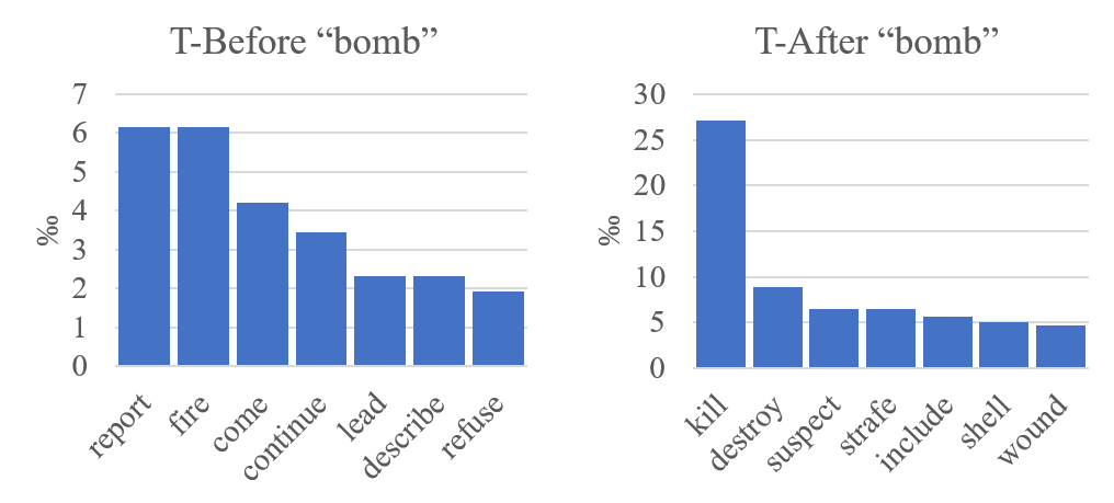
(b) bomb

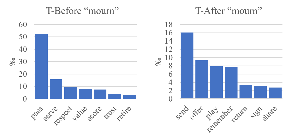
(c) mourn

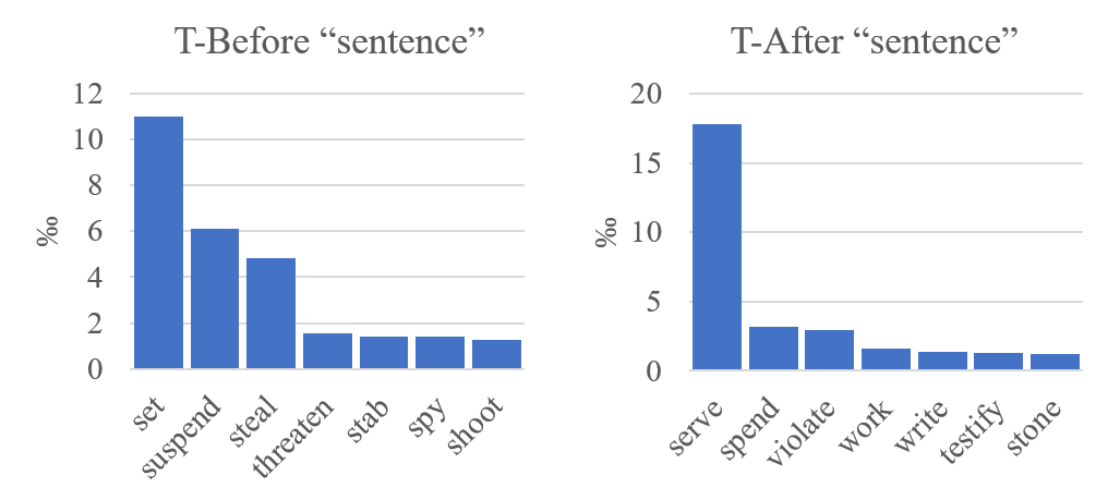
(d) sentence

Figure 1: Top events that most frequently precede or follow “investigate”, “bomb”, “mourn”, or “sentence” in time, sorted by their conditional probabilities in ‰. Word senses have been disambiguated and the “bomb” and “sentence” here are their verb meanings. There are some possible errors (e.g., report is T-Before bomb) and some unclear pairs (e.g., know is T-Before investigate and play is T-After mourn), but overall the event sequences discovered here are reasonable. More examples can be found in the appendix.

3.4.2 Distribution of Following Events

For each verb $v$, we define the marginal count of $v$ being P-Before to arbitrary verbs with TempRel $r\in R$ as $C(v,r)=\sum_{v_{i}\in V}C(v,v_{i},r)$. Then for every other verb $v^{\prime}$, we define

$$P(v~{}\textrm{T-Before}~{}v^{\prime}|v~{}\textrm{T-Before})\triangleq\frac{C(v,v^{\prime},before)}{C(v,before)},$$ (3)

which is the probability of $v$ T-Before $v^{\prime}$, conditioned on $v$ T-Before anything. Similarly, we define

$$P(v~{}\textrm{T-After}~{}v^{\prime}|v~{}\textrm{T-After})\triangleq\frac{C(v,v^{\prime},after)}{C(v,after)}.$$ (4)

For a specific verb, e.g., $v$=investigate, each verb $v^{\prime}\in V$ is sorted by the two conditional probabilities above. Then the most probable verbs that temporally precede or follow $v$ are shown in Fig. 1, where the y-axes are the corresponding conditional probabilities. We can see reasonable event sequences like {involve, kill, suspect, steal}$\to$investigate$\to${report, prosecute, pay, punish}, which indicates the possibility of using TemProb for event sequence predictions or story cloze tasks. There are also suspicious pairs like know in the T-Before list of investigate (Fig. 1a), report in the T-Before list of bomb (Fig. 1b), and play in the T-After list of mourn (Fig. 1c). Since the arguments of these verb frames are not considered here, whether these few seemingly counter-intuitive pairs come from system error or from a special context needs further investigation.

4 Experiments

In the above, we have explained the construction of TemProb and shown some interesting examples from it, which were meant to visualize its correctness. In this section, we first quantify the correctness of the prior obtained in TemProb, and then show TemProb can be used to improve existing TempRel extraction systems.

4.1 Quality Analysis of TemProb

In Table 2, we showed examples with either $\eta_{b}$ or $\eta_{a}>0.9$. We argued that they seem correct. Here we quantify the “correctness” of $\eta_{b}$ and $\eta_{a}$ based on TBDense. Specifically, we collected all the gold T-Before and T-After pairs. Let $\tau\in[0.5,1)$ be a constant threshold. Imagine a naive predictor such that for each pair of events $v_{i}$ and $v_{j}$, if $\eta_{b}>\tau$, it predicts that $v_{i}$ is T-Before $v_{j}$; if $\eta_{a}>\tau$, it predicts that $v_{i}$ is T-After $v_{j}$; otherwise, it predicts that $v_{i}$ is T-Vague to $v_{j}$. We expect that a higher $\eta_{b}$ (or $\eta_{a}$) represents a higher confidence for an instance to be labeled T-Before (or T-After).

Table 3: Validating $\eta_{b}$ and $\eta_{a}$ from TemProb based on the T-Before and T-After examples in TBDense. Performances are decomposed into same sentence examples (Dist=0) and contiguous sentence examples (Dist=1). A larger threshold leads to a higher precision, so $\eta_{b}$ and $\eta_{a}$ indeed represent a notion of confidence.

Threshold $\tau$	Dist=0		Dist=1
	P	R	P	R
0.5	65.6	61.3	58.5	53.3
0.6	69.8	44.5	60.5	36.9
0.7	74.6	29.2	63.6	18.7
0.8	81.0	13.9	64.8	6.9
0.9	82.9	5.0	76.9	1.2

Table 3 shows the performance of this predictor, which meets our expectation and thus justifies the validity of TemProb. As we gradually increase the value of $\tau$ in Table 3, the precision increases in roughly the same pace with $\tau$, which indicates that the values of $\eta_{b}$ and $\eta_{a}$ from TemProb indeed represent the confidence level. The decrease in recall is also expected because more examples are labeled as T-Vague when $\tau$ is larger.

To further justify the quality, we also used another dataset that is not in the TempRel domain. Instead, we downloaded the EventCausality dataset Do et al. (2011). For each causally related pair e1 and e2, if EventCausality annotates that e1 causes e2, we changed it to be T-Before; if EventCausality annotates that e1 is caused by e2, we changed it to be T-after. Therefore, based on the assumption that the cause event is T-Before the result event, we converted the EventCausality dataset to be a TempRel dataset and it thus could also be used to evaluate the quality of TemProb. We adopted the same predictor used in Table 3 with $\tau=0.5$ and in Table 4, we compared it with two baselines: (i) always predicting T-Before and (ii) always predicting T-After. First, the accuracy (66.2%) in Table 4 is rather consistent with its counterpart in Table 3, confirming the stability of statistics from TemProb. Second, by directly using the prior statistics $\eta_{b}$ and $\eta_{a}$ from TemProb, we can improve the precision of both labels with a significant margin relative to the two baselines (17.0% for “T-Before” and 15.9% for “T-After”). Overall, the accuracy was improved by 11.5%.

Table 4: Further justification of $\eta_{b}$ and $\eta_{a}$ from TemProb on the EventCausality dataset. The thresholding predictor from Table 3 with $\tau=0.5$ is used here. Compared to always predicting the majority label (i.e., T-Before in this case), $\tau=0.5$ significantly improved the performance for both labels, with the overall accuracy improved by 11.5%.

System	T-Before		T-After		Acc.
	P	R	P	R
T-Before Only	54.7	100.0	0	0	54.7
T-After Only	0	0	45.3	100	45.3
$\tau=0.5$	71.7	63.3	61.2	69.8	66.2

4.2 Improving TempRel Extraction

The original purpose of TemProb was to improve TempRel extraction. We show it from two perspectives: How effective the prior distributions obtained from TemProb are (i) as features in local methods and (ii) as regularization terms in global methods. The results below were evaluated on the test split of TB-Dense Cassidy et al. (2014).

4.2.1 Improving Local Methods

We first test how well the prior distributions from TemProb can be used as features in improving local methods for TempRel extraction. In Table 5, we used the original feature set proposed in Sec. 3.2.1 as the baseline, and added the prior distribution obtained from TemProb on top of it. Specifically, we added $\eta_{b}$ (see Eq. (1)) and $\{f_{r}\}_{r\in R}$, respectively, where $\{f_{r}\}_{r\in R}$ is the prior distributions of all labels, i.e.,

$$f_{r}(v_{i},v_{j})=\frac{C(v_{i},v_{j},r)}{\sum_{r^{\prime}\in R}{C(v_{i},v_{j},r^{\prime})}},~{}r\in R.$$ (5)

Recall function $C$ is defined in Eq. (2). All comparisons were decomposed to same sentence relations (Dist=0) and neighboring sentence relations (Dist=1) for a better understanding of the behavior. All classifiers were trained using the averaged perceptron algorithm Freund and Schapire (1998) and tuned by 3-fold cross validation.

From Table 5, we can see that simply adding $\eta_{b}$ into the feature set could improve the original system F₁ by 1.8% (Dist=0) and 3.0% (Dist=1). If we further add as features the full set of prior distributions $\{f_{r}\}_{r\in R}$, the improvement comes to 2.7% and 6.5%, respectively. Noticing that the feature is more helpful for Dist=1, we think that it is because distant pairs usually have less lexical dependency and thus need more prior information provided by our new feature. With Dist=0 and Dist=1 combined (numbers not shown in the Table), the 3rd line improved the ”original” by 4.7% in F₁ and by 5.1% in the temporal awareness F-score (another metric used in the TempEval3 workshop).

Table 5: Using prior distributions derived from TemProb as features in an example local method. Incorporating $\eta_{b}$ to the original feature set already yields better performance. By using the full set of prior distributions, $\{f_{r}\}_{r\in R}$, the final system improves the original in almost all metrics, and the improvement is statistically significant with p$<$0.005 per the McNemar’s test.

Feature Set	Dist=0			Dist=1
	P	R	F1	P	R	F1
Original	44.5	57.1	50.0	49.0	36.9	42.1
+$\eta_{b}$	46.2	58.9	51.8	55.3	38.1	45.1
+$\{f_{r}\}_{r\in R}$	46.9	60.1	52.7	51.3	46.2	48.6

• Note The performances here are consistently lower than those in Table 3 because in Table 3, only T-Before and T-After examples are considered, but here all labels are taken into account and the problem is more practical and harder.

4.2.2 Improving Global Methods

As mentioned earlier in Sec. 2, many systems adopt a global inference method via integer linear programming (ILP) Roth and Yih (2004) to enforce transitivity constraints over an entire temporal graph Bramsen et al. (2006); Chambers and Jurafsky (2008); Denis and Muller (2011); Do et al. (2012); Ning et al. (2017). In addition to the usage shown in Sec. 4.2.1, the prior distributions from TemProb can also be used to regularize the conventional ILP formulation. Specifically, in each document, let $\mathcal{I}_{r}(ij)\in\{0,1\}$ be the indicator function of relation $r$ for event $i$ and event $j$; let $x_{r}(ij)\in[0,1]$ be the corresponding soft-max score obtained from the local classifiers (depending on the sentence distance between $i$ and $j$). Then the ILP objective for global inference is formulated as follows.

$$\hat{\mathcal{I}}=\textrm{arg}\underset{\mathcal{I}}{\textrm{max}}\sum_{ij\in\mathcal{E}}\sum_{r\in R}(x_{r}(ij)+\underline{\lambda f_{r}(ij)})\mathcal{I}_{r}(ij)$$ (6)

$$\textrm{s.t.}\quad\underset{\textrm{(uniqueness)}}{\Sigma_{r}{\mathcal{I}_{r}(ij)}=1},~{}\underset{\textrm{(symmetry)}}{\mathcal{I}_{r}(ij)=\mathcal{I}_{\bar{r}}(ji),}$$

$$\underset{\textrm{(transitivity)}}{\mathcal{I}_{r_{1}}(ij)+\mathcal{I}_{r_{2}}(jk)-\Sigma_{m=1}^{M}\mathcal{I}_{r_{3}^{m}}(ik)\leq 1,}$$

for all distinct events $i$, $j$, and $k$, where $\mathcal{E}=\{ij~{}|~{}\textrm{sentence dist$(i,j)$$\leq 1$}\}$, $\lambda$ adjusts the regularization term and was heuristically set to 0.5 in this work, $\bar{r}$ is the reverse relation of $r$, and $M$ is the number of possible relations for $r_{3}$ when $r_{1}$ and $r_{2}$ are true. Note our difference from the ILP in Ning et al. (2017) is the underlined regularization term $f_{r}(ij)$ (which itself is defined in Eq. (5)) obtained from TemProb.

Table 6: Regularizing global methods by the prior distribution derived from TemProb. The “+” means adding a component on top of its preceding line. F${}_{\text{aware}}$ is the temporal awareness F-score, another evaluation metric used in TempEval3. The baseline system is to use (unregularized) ILP on top of the original system in Table 5. System 3 is the proposed. Per the McNemar’s test, System 3 is significantly better than System 1 with p$<$0.0005.

No.	System	P	R	F1	F${}_{\text{aware}}$
1	Baseline	48.1	44.4	46.2	42.5
2	+Feature: $\{f_{r}\}_{r\in R}$	50.6	52.0	51.3	49.1
3	+Regularization	51.3	53.0	52.1	49.6

We present our results on the test split of TB-Dense in Table 6, which is an ablation study showing step-by-step improvements in two metrics. In addition to the straightforward precision, recall, and F₁ metric, we also compared the F₁ of the temporal awareness metric used in TempEval3 UzZaman et al. (2013). The awareness metric performs graph reduction and closure before evaluation so as to better capture how useful a temporal graph is. Details of this metric can be found in UzZaman and Allen (2011); UzZaman et al. (2013); Ning et al. (2017).

Table 7: Label-wise performance improvement of System 3 over System 1 in Table 6. We can see that incorporating TemProb improves the recall of before and after, and improves the precision of all labels, with a slight drop in the recall of vague.

Label	P	R	F1
before	+0.3	+15	+6
after	+4	+4	+4
equal	+11	0	+2
includes	+17	0	+0.2
included	+8	0	+2
vague	+3	-4	-1

In Table 6, the baseline used the original feature set proposed in Sec. 3.2.1 and applied global ILP inference with transitivity constraints. Technically, it is to solve Eq. (6) with $\lambda=0$ (i.e., unregularized) on top of the original system in Table 5. Apart from some implementation details, this baseline is also the same as many existing global methods as Chambers and Jurafsky (2008); Do et al. (2012). System 2, “+Feature: $\{f_{r}\}_{r\in R}$”, is to add prior distributions as features when training the local classifiers. Technically, the scores $x_{r}(ij)$’s in Eq. (6) used by baseline were changed. We know from Table 5 that adding $\{f_{r}\}_{r\in R}$ made the local decisions better. Here the performance of System 2 shows that this was also the case for the global decisions made via ILP: both precision and recall got improved, and F₁ and awareness were both improved by a large margin, with 5.1% in F₁ and 6.6% in awareness F₁. On top of this, System 3 sets $\lambda=0.5$ in Eq. (6) to add regularizations to the conventional ILP formulation. The sum of these regularization terms represents a confidence score of how coherent the predicted temporal graph is to our TemProb, which we also want to maximize. Even though a considerable amount of information from TemProb had already been encoded as features (as shown by the large improvements by System 2), these regularizations were still able to further improve the precision, recall and awareness scores. To sum up, the total improvement over the baseline system brought by TemProb is 5.9% in F₁ and 7.1% in awareness F₁, both with a notable margin. Table 7 furthermore decomposes this improvement into each TempRel label.

Table 8: Comparison of the proposed TempRel extraction method with two best-so-far systems in terms of two metrics. Since TemProb is only on verb events extracted by SRL, Partial TBDense is the focus of our work, where we can see significant improvement brought by simply using the prior knowledge from TemProb. Per the McNemar’s test, Line 3 is better than Line 2 with p$<$0.0005. For interested readers, we also naively augmented the proposed method to the complete TBDense and show state-of-the-art performance on it.

No.	System	P	R	F1	F${}_{\text{aware}}$
Partial TBDense*: Focus of this work.
1	CAEVO	52.3	43.7	47.6	46.7
2	Ning et al. (2017)	47.4	56.3	51.5	49.1
3	Proposed	50.0	62.4	55.5	52.8
Complete TBDense: Naive augmentation.
4	CAEVO	51.8	32.6	40.0	45.7
5	Ning et al. (2017)	46.2	40.6	43.2	48.5
6	Proposed**	47.2	42.4	44.7	49.2

• *Note that TemProb is only available for events extracted by SRL (See Sec. 3.2.2 for details).

• **Augment the output of Line 3 with predictions from Ning et al. (2017).

To compare with state-of-the-art systems, which all used gold event properties (i.e., Tense, Aspect, Modality, and Polarity), we retrained System 3 in Table 6 with these gold properties and show the results in Table 8. We reproduced the results of CAEVO Chambers et al. (2014) and Ning et al. (2017) and evaluated them on the partial TBDense test split. Under both metrics, the proposed system achieved the best performance. An interesting fact is that even without these gold properties, our System 3 in Table 6 was already better than CAEVO (on Line 1) and Ning et al. (2017) (on Line 2) in both metrics. This is appealing because in practice, those gold properties may not exist, but our proposed system can still generate state-of-the-art performance without them.

For readers who are interested in the complete TBDense dataset, we also performed a naive augmentation as follows. Recall that System 3 only makes predictions to a subset of the complete TBDense dataset. We kept this subset of predictions, and filled the missing predictions by Ning et al. (2017). Performances of this naively augmented proposed system is compared with CAEVO and Ning et al. (2017) on the complete TBDense dataset. We can see that by replacing with predictions from our proposed system, Ning et al. (2017) got a better precision, recall, F₁, and awareness F₁, which is the new state-of-the-art on all reported performances on this dataset. Note that the awareness F₁ scores on Lines 4-5 are consistent with reported values in Ning et al. (2017). To our knowledge, the results in Table 8 is the first in literature that reports performances in both metrics, and it is promising to see that the proposed method outperformed state-of-the-art methods in both metrics.

5 Conclusion

Temporal relation (TempRel) extraction is an important and challenging task in NLP, partly due to its strong dependence on prior knowledge. Motivated by practical examples, this paper argues that a resource of the temporal order that events usually follow is helpful. To construct such a resource, we automatically processed a large corpus from NYT with more than 1 million documents using an existing TempRel extraction system and obtained the TEMporal relation PRObabilistic knowledge Base (TemProb). The TemProb is a good showcase of the capability of such prior knowledge, and it has shown its power in improving existing TempRel extraction systems on a benchmark dataset, TBDense. The resource and the system reported in this paper are both publicly available and we hope that it can foster more investigations into time-related tasks.

Appendix A Supplemental Material

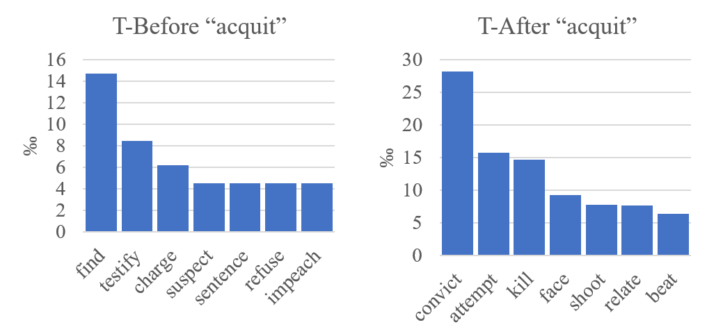
(a) acquit

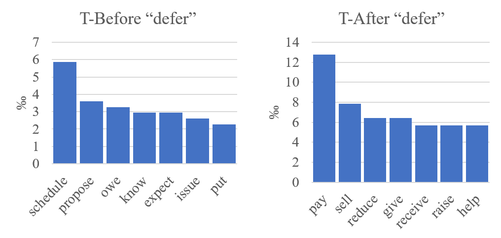
(b) defer

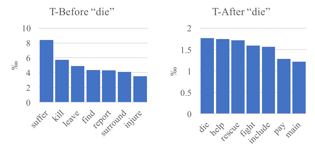
(c) die

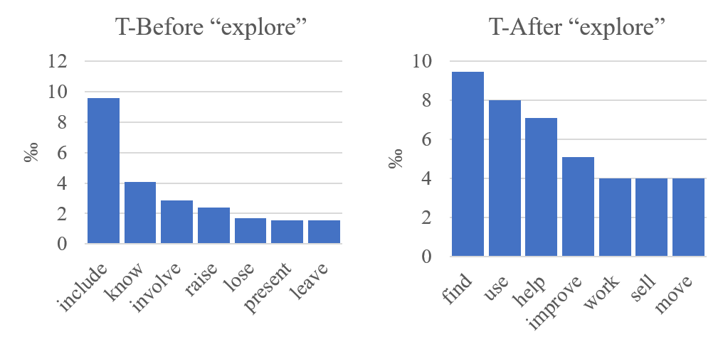
(d) explore

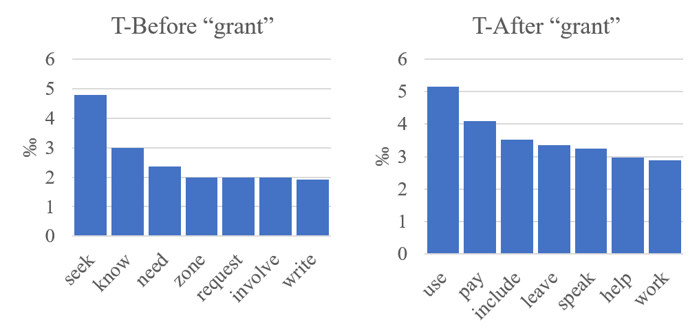
(e) grant

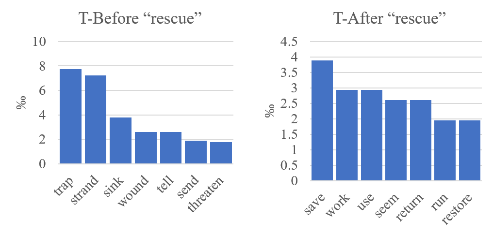
(f) rescue

Figure 2: A few more examples in addition to Fig. 1.

In Sec. 3.4.2, we have shown some interesting examples with events that temporally precede or follow a certain event. In addition to those examples shown in Fig. 1, it is actually very easy to find more interesting examples. We have picked some and shown them in Fig. 2. Again, there are potential errors in these figures, but the overall quality is intuitively appealing.

In Sec. 4.1, we have shown the quality analysis of TemProb in Tables 3-4 via the TimeBank-Dense dataset Cassidy et al. (2014) and the EventCausality dataset Do et al. (2011). Here we further provide confidence level analysis on some randomly selected event pairs. Specifically, we performed a 10-fold bootstrapping. In each fold, we randomly selected 50% of the graphs in TemProb (i.e., from $\{G_{i}\}_{i=1}^{N}$) with replacement. Then we re-calculated the prior statistics $\{f_{r}(v_{i},v_{j})\}$ (Eq. (5)) in each fold. By considering $\{f_{r}(v_{i},v_{j})\}$ as a random variable, we now obtained 10 realizations of it, so we can evaluate the confidence level. In Fig. 3 (with color), we show the confidence levels of several randomly selected pairs of events. From Fig. 3, we can see that the prior statistics are actually rather stable, indicating that the prior statistics represented by TemProb is indeed a notion of knowledge underlying natural language text.

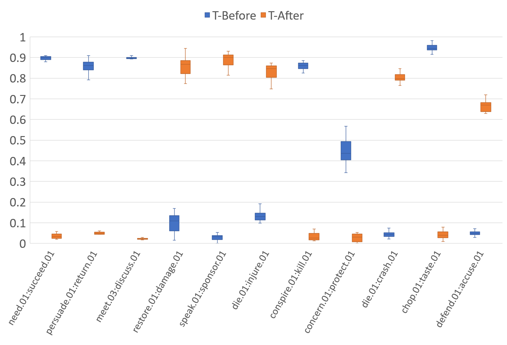
Figure 3: Confidence intervals from 10-fold bootstrapping.

References

- Bethard et al. (2015) Steven Bethard, Leon Derczynski, Guergana Savova, James Pustejovsky, and Marc Verhagen. 2015. SemEval-2015 Task 6: Clinical TempEval. In Proceedings of the 9th International Workshop on Semantic Evaluation (SemEval 2015). Association for Computational Linguistics, Denver, Colorado, pages 806–814.
- Bethard et al. (2007) Steven Bethard, James H Martin, and Sara Klingenstein. 2007. Timelines from text: Identification of syntactic temporal relations. In IEEE International Conference on Semantic Computing (ICSC). pages 11–18.
- Bethard et al. (2016) Steven Bethard, Guergana Savova, Wei-Te Chen, Leon Derczynski, James Pustejovsky, and Marc Verhagen. 2016. SemEval-2016 Task 12: Clinical TempEval. In Proceedings of the 10th International Workshop on Semantic Evaluation (SemEval-2016). Association for Computational Linguistics, San Diego, California, pages 1052–1062.
- Bethard et al. (2017) Steven Bethard, Guergana Savova, Martha Palmer, and James Pustejovsky. 2017. SemEval-2017 Task 12: Clinical TempEval. In Proceedings of the 11th International Workshop on Semantic Evaluation (SemEval-2017). Association for Computational Linguistics, pages 565–572.
- Bollacker et al. (2008) Kurt Bollacker, Colin Evans, Praveen Paritosh, Tim Sturge, and Jamie Taylor. 2008. Freebase: a collaboratively created graph database for structuring human knowledge. In Proceedings of the 2008 ACM SIGMOD international conference on Management of data. ACM, pages 1247–1250.
- Bramsen et al. (2006) P. Bramsen, P. Deshpande, Y. K. Lee, and R. Barzilay. 2006. Inducing temporal graphs. In Proceedings of the Conference on Empirical Methods for Natural Language Processing (EMNLP). pages 189–198.
- Cassidy et al. (2014) Taylor Cassidy, Bill McDowell, Nathanel Chambers, and Steven Bethard. 2014. An annotation framework for dense event ordering. In Proceedings of the Annual Meeting of the Association for Computational Linguistics (ACL). pages 501–506.
- Chambers and Jurafsky (2008) N. Chambers and D. Jurafsky. 2008. Jointly combining implicit constraints improves temporal ordering. In Proceedings of the Conference on Empirical Methods for Natural Language Processing (EMNLP).
- Chambers et al. (2014) Nathanael Chambers, Taylor Cassidy, Bill McDowell, and Steven Bethard. 2014. Dense event ordering with a multi-pass architecture. Transactions of the Association for Computational Linguistics 2:273–284.
- Chambers et al. (2007) Nathanael Chambers, Shan Wang, and Dan Jurafsky. 2007. Classifying temporal relations between events. In Proceedings of the 45th Annual Meeting of the ACL on Interactive Poster and Demonstration Sessions. pages 173–176.
- Chklovski and Pantel (2004) T. Chklovski and P. Pantel. 2004. VerbOcean: Mining the Web for Fine-Grained Semantic Verb Relations. In Proceedings of the Conference on Empirical Methods for Natural Language Processing (EMNLP). pages 33–40.
- Clarke et al. (2012) J. Clarke, V. Srikumar, M. Sammons, and D. Roth. 2012. An nlp curator (or: How i learned to stop worrying and love nlp pipelines). In Proc. of the International Conference on Language Resources and Evaluation (LREC).
- Denis and Muller (2011) Pascal Denis and Philippe Muller. 2011. Predicting globally-coherent temporal structures from texts via endpoint inference and graph decomposition. In Proceedings of the International Joint Conference on Artificial Intelligence (IJCAI). volume 22, page 1788.
- Do et al. (2011) Q. Do, Y. Chan, and D. Roth. 2011. Minimally supervised event causality identification. In Proc. of the Conference on Empirical Methods in Natural Language Processing (EMNLP). Edinburgh, Scotland.
- Do et al. (2012) Q. Do, W. Lu, and D. Roth. 2012. Joint inference for event timeline construction. In Proc. of the Conference on Empirical Methods in Natural Language Processing (EMNLP).
- Fellbaum (1998) C. Fellbaum. 1998. WordNet: An Electronic Lexical Database. MIT Press.
- Freund and Schapire (1998) Y. Freund and R. Schapire. 1998. Large margin classification using the Perceptron algorithm. In Proceedings of the Annual ACM Workshop on Computational Learning Theory (COLT). pages 209–217.
- Graff (2002) David Graff. 2002. The AQUAINT corpus of english news text. Linguistic Data Consortium, Philadelphia .
- Hoffart et al. (2013) Johannes Hoffart, Fabian M. Suchanek, Klaus Berberich, and Gerhard Weikum. 2013. Yago2: A spatially and temporally enhanced knowledge base from wikipedia (extended abstract). In Proceedings of the International Joint Conference on Artificial Intelligence (IJCAI).
- Hovy et al. (2013) Eduard Hovy, Teruko Mitamura, Felisa Verdejo, Jun Araki, and Andrew Philpot. 2013. Events are not simple: Identity, non-identity, and quasi-identity. In Workshop on Events.
- Jiang et al. (2016) Tingsong Jiang, Tianyu Liu, Tao Ge, Lei Sha, Baobao Chang, Sujian Li, and Zhifang Sui. 2016. Towards time-aware knowledge graph completion. In Proceedings of COLING 2016, the 26th International Conference on Computational Linguistics: Technical Papers. The COLING 2016 Organizing Committee, Osaka, Japan, pages 1715–1724.
- Llorens et al. (2015) Hector Llorens, Nathanael Chambers, Naushad UzZaman, Nasrin Mostafazadeh, James Allen, and James Pustejovsky. 2015. SemEval-2015 Task 5: QA TEMPEVAL - evaluating temporal information understanding with question answering. In Proceedings of the 9th International Workshop on Semantic Evaluation (SemEval 2015). pages 792–800.
- Mani et al. (2006) Inderjeet Mani, Marc Verhagen, Ben Wellner, Chong Min Lee, and James Pustejovsky. 2006. Machine learning of temporal relations. In Proceedings of the Annual Meeting of the Association for Computational Linguistics (ACL). pages 753–760.
- Minard et al. (2015) Anne-Lyse Minard, Manuela Speranza, Eneko Agirre, Itziar Aldabe, Marieke van Erp, Bernardo Magnini, German Rigau, Ruben Urizar, and Fondazione Bruno Kessler. 2015. SemEval-2015 Task 4: TimeLine: Cross-document event ordering. In Proceedings of the 9th International Workshop on Semantic Evaluation (SemEval 2015). pages 778–786.
- Mirza and Tonelli (2016) Paramita Mirza and Sara Tonelli. 2016. CATENA: CAusal and TEmporal relation extraction from NAtural language texts. In The 26th International Conference on Computational Linguistics. pages 64–75.
- Mitamura et al. (2015) T. Mitamura, Y. Yamakawa, S. Holm, Z. Song, A. Bies, S. Kulick, and S. Strassel. 2015. Event nugget annotation: Processes and issues. In Proceedings of the Workshop on Events at NAACL-HLT.
- Ning et al. (2017) Qiang Ning, Zhili Feng, and Dan Roth. 2017. A structured learning approach to temporal relation extraction. In Proceedings of the Conference on Empirical Methods for Natural Language Processing (EMNLP). Copenhagen, Denmark.
- Peng and Roth (2016) Haoruo Peng and Dan Roth. 2016. Two discourse driven language models for semantics. In Proc. of the Annual Meeting of the Association for Computational Linguistics (ACL).
- Peng et al. (2016) Haoruo Peng, Yangqiu Song, and Dan Roth. 2016. Event detection and co-reference with minimal supervision. In Proc. of the Conference on Empirical Methods in Natural Language Processing (EMNLP).
- Pustejovsky et al. (2003) James Pustejovsky, Patrick Hanks, Roser Sauri, Andrew See, Robert Gaizauskas, Andrea Setzer, Dragomir Radev, Beth Sundheim, David Day, Lisa Ferro, et al. 2003. The TIMEBANK corpus. In Corpus linguistics. volume 2003, page 40.
- Rizzolo and Roth (2010) N. Rizzolo and D. Roth. 2010. Learning based java for rapid development of nlp systems. In Proc. of the International Conference on Language Resources and Evaluation (LREC). Valletta, Malta.
- Roth and Yih (2004) D. Roth and W. Yih. 2004. A linear programming formulation for global inference in natural language tasks. In Hwee Tou Ng and Ellen Riloff, editors, Proc. of the Conference on Computational Natural Language Learning (CoNLL). pages 1–8.
- Song et al. (2015) Zhiyi Song, Ann Bies, Stephanie Strassel, Tom Riese, Justin Mott, Joe Ellis, Jonathan Wright, Seth Kulick, Neville Ryant, and Xiaoyi Ma. 2015. From light to rich ere: Annotation of entities, relations, and events. In Proceedings of the The 3rd Workshop on EVENTS: Definition, Detection, Coreference, and Representation. Association for Computational Linguistics, Denver, Colorado, pages 89–98.
- Spiliopoulou et al. (2017) Evangelia Spiliopoulou, Eduard Hovy, and Teruko Mitamura. 2017. Event detection using frame-semantic parser. In Proceedings of the Events and Stories in the News Workshop. Association for Computational Linguistics, Vancouver, Canada, pages 15–20.
- UzZaman and Allen (2011) Naushad UzZaman and James F Allen. 2011. Temporal evaluation. In Proceedings of the Annual Meeting of the Association for Computational Linguistics (ACL). pages 351–356.
- UzZaman et al. (2013) Naushad UzZaman, Hector Llorens, James Allen, Leon Derczynski, Marc Verhagen, and James Pustejovsky. 2013. SemEval-2013 Task 1: TempEval-3: Evaluating time expressions, events, and temporal relations. In Second Joint Conference on Lexical and Computational Semantics. volume 2, pages 1–9.
- Verhagen et al. (2007) Marc Verhagen, Robert Gaizauskas, Frank Schilder, Mark Hepple, Graham Katz, and James Pustejovsky. 2007. SemEval-2007 Task 15: TempEval temporal relation identification. In SemEval. pages 75–80.
- Verhagen and Pustejovsky (2008) Marc Verhagen and James Pustejovsky. 2008. Temporal processing with the TARSQI toolkit. In 22nd International Conference on on Computational Linguistics: Demonstration Papers. pages 189–192.
- Verhagen et al. (2010) Marc Verhagen, Roser Sauri, Tommaso Caselli, and James Pustejovsky. 2010. SemEval-2010 Task 13: TempEval-2. In SemEval. pages 57–62.