OCU-PHYS-477

Revisiting Electroweak Symmetry Breaking and
Higgs Mass in Gauge-Higgs Unification

Yuki Adachi and Nobuhito Maru^∗

Department of Sciences, Matsue College of Technology, Matsue 690-8518, Japan.

^∗ Department of Mathematics and Physics, Osaka City University, Osaka 558-8585, Japan.

Abstract

We propose a new model of 5D $SU(3)\otimes U(1)_{X}$ gauge-Higgs unification with a successful electroweak symmetry breaking and a realistic Higgs boson mass. In our model, the representations of the fermions are very simple, the $\bf 3,\bar{\bf 3}$ and $\overline{\bf 15}$ representations of $SU(3)$ gauge group. Employing the anti-periodic boundary conditions for $\overline{\bf 15}$ reduces massless exotic fermions and simplifies the brane localized mass terms. We calculate the 1-loop Higgs potential in detail and find that a realistic electroweak symmetry breaking and the observed Higgs mass are obtained.

1 Introduction

Gauge-Higgs unification (GHU) [1, 2] unifies the standard model (SM) gauge boson and Higgs boson into the higher dimensional gauge fields. This scenario is one of the attractive ideas that solves the hierarchy problem without invoking supersymmetry, since the Higgs boson mass and its potential are calculable due to the higher dimensional gauge symmetry [2]. These characteristic features have been studied and verified in models with various types of compactification at one-loop level [3] and at the two-loop level [4]. The calculability of other physical observables such as $S$ and $T$ parameters [5], Higgs couplings to digluons, diphotons [6], muon $g-2$ and the EDM of neutron [7] have been also investigated. The flavor physics which is a very nontrivial in GHU has been studied in [8].

In five dimensional (5D) GHU, Higgs potential at the tree level is forbidden by the gauge symmetry in higher dimensions, but it is radiatively generated. Due to its characteristic features, it is nontrivial to obtain a realistic electroweak symmetry breaking and the observed Higgs mass. In GHU, Higgs quartic coupling is provided by the gauge coupling squared and is 1-loop suppressed. Therefore, Higgs mass squared is naively of order 1-loop factor times the compactification scale squared $m_{h}^{2}\sim\frac{1}{16\pi^{2}R^{2}}$. Noting that W boson mass and the compactification scale are related by $M_{W}=c/R$ in terms of a dimensionless parameter “$c$” which is determined from the potential minimum, Higgs mass is too small if the parameter $c$ is an order of the unity [9]. If we manage to realize a small parameter $c$ by potential minimization, this allows the larger compactification scale and heavier Higgs mass. In order to obtain a small parameter $c$, it is well-known that it has to be generated by the contributions from different representations of the gauge group.

It is troublesome to eliminate the massless exotic fermions. Embedding the SM fermions into the large representations, there exist many massless exotic fermions and they are ordinary made massive by introducing the brane mass terns and extra brane localized fermions coupling to Dirac mass with the exotic fermions. Even for the $SU(2)$ SM doublets, the number of massless doublets is duplicated in each generation since massless doublets appear from the isospin up and down components. To eliminate the half of the massless doublets, we also must introduce the brane mass terms and extra brane localized doublets coupling to Dirac mass with the exotic massless doublets. Such brane mass terms complicate models and analysis. Therefore, it is desirable to construct a model where the brane mass terms are as little as possible.

In this paper, we propose a new model of 5D $SU(3)\otimes U(1)_{X}$ GHU with a successful electroweak symmetry breaking and a realistic Higgs boson mass. In our model, the representations of the fermions are only two kinds, that is, the $\bf 3,\overline{\bf 15}$ for the third generation quarks and $\bf 3\oplus\bar{\bf 3}$ representations of $SU(3)$ gauge group for other SM fermions. In our setup, top quark is not embedded into the $\overline{\bf 15}$ representations. In this case, we have no need to obtain massless zero mode from the bulk fermions and we can impose the anti-periodic boundary conditions for $\overline{\bf 15}$. Therefore, we have no need to introduce the brane localized mass terms since the lightest mode is necessarily massive. From the fundamental representations, the massless exotic $SU(2)_{L}$ doublets are unavoidable because these massless doublets appear from the up- and down-type sectors. Namely, the number of the massless $SU(2)_{L}$ doublets are doubled. We have to introduce the brane mass terms for one linear combinations of doublets to make them massive.

We calculate the 1-loop Higgs potential and search a viable matter content to realize a realistic electroweak symmetry breaking and the observed Higgs mass. In order to accomplish this, it is found that a pair of additional $\overline{\bf 15}$ representations other than the SM fermions should be included. We also study whether the top and bottom quark masses are reproduced. Note that the masses of $SU(2)_{L}$ doublets are correlated through the mixing between the $SU(2)_{L}$ doublets from the up- and down-type sectors . For the third generation quarks, it is not a trivial issue since the mass difference between top and bottom is larger than those of the first two generations.

This paper is organized as follows. In section 2, we describe our model. In section 3, we calculate the mass spectrum of the various fields introduced in our model. The Higgs potential is calculated and analyzed in section 4. Summary is devoted to section 5. In appendix, the details of several representations are summarized.

2 A model

We consider the $SU(3)\otimes U(1)_{X}$ gauge theory in five-dimensional flat space-time. The fifth extra dimension is compactified on an orbifold $S^{1}/Z_{2}$ where the radius of $S^{1}$ is $R$. Because the weak mixing angle $\theta_{W}$ in the $SU(3)$ is not consistent with the realistic one, the correct value is effectively realized by the mixing between the $U(1)_{X}$ and neutral gauge bosons of $SU(3)$.

The SM chiral fermions are introduced as follows: The top quark ($t$) and the bottom quark ($b$) quarks are brane-localized fermions localized at the $y=\pi R$ brane. Other SM fermions are embedded in the bulk fermions $\Psi_{l}$ and $\Psi_{q}$. They obtain a mass through the five-dimensional gauge interaction as ordinary way in the context of the gauge-Higgs unification scenario. Since the $t$ and $b$ quarks cannot interact directly with Higgs boson ($A_{y}$), the extra bulk fermions $\Psi$ (referred to as messenger fermions) are necessary to connect them. We also introduce a pair of fermions (referred to as mirror fermions) $\Psi_{\rm M}$ and $X_{\rm M}$ to realize the realistic electroweak symmetry breaking. Such fermions may be a possible candidate of the dark matter as pointed out in [10]. The outline of this model is depicted in the Figure 1. Such a strategy simplifies our model: The top quark needs a large representation to reproduce the large top yukawa coupling as will be mentioned in the following sections. In general, such a large representation includes the massless exotic fermions but they are automatically removed from the low-energy effective theory by use of the anti-periodic boundary condition. The other light fermions are embedded in the fundamental representations to assign the suitable $U(1)_{X}$ charges. Thus the extra brane fermions and brane mass terms are greatly reduced in our model.

Figure 1: Setup of the model.

Since the gauge sectors of our model has been discussed in detail [11], we focus on the the fermion sector in the following subsections.

2.1 The third generation quark

In this subsection, we discuss the $t$ and $b$ quarks. As is mentioned in the previous paragraph, the third generation $t_{R},b_{R}$ and $\begin{pmatrix}t_{L}\\ b_{L}\end{pmatrix}$ are put on the $y=\pi R$ brane. The chirality is defined as the eigenvalues of the chiral projection operators $L=(1-\gamma_{5})/2,R=(1+\gamma_{5})/2$. As for the messenger fermion, the $\bf 3_{0}$ and $\overline{\bf 15}_{\bf-2/3}$ representations are introduced. The subscripts stand for the $U(1)_{X}$ charges in order to couple with the brane fermions. These messenger fermions include the two quark doublets $Q_{3},Q_{15}$ and the two singlets $B,T$.

We impose the $Z_{2}$ symmetry and anti-periodic boundary condition on the messenger fermions to leave the chiral fermions:

$$\Psi(y+2\pi R)=-\Psi(y),\quad\Psi(y)=-P\gamma_{5}\Psi(-y)$$ (2.1)

where the matrix $P$ is defined as $P=\text{diag}(++-)$ for the $SU(3)$ fundamental representation. Due to such an anti-periodic boundary condition, they obtain a mass at least around $1/(2R)$, so the exotic fermions are automatically removed from the low energy effective theory. Since the $Z_{2}$ parities at $y=\pi R$ is opposite to those of the $y=0$ because of the anti-periodicity, the right-handed doublet and left-handed singlet in the messenger fermion can couple to the SM fermions ($t$ and $b$ quarks) at $y=\pi R$. The Lagrangian of the third generation quarks becomes

$$\mathcal{L}_{\text{fermion}}\supset \bar{\psi}({\bf 3_{0}})i\!\!\not\!\!D_{{\bf 3}}\psi({\bf 3_{0}})+\bar{\psi}(\overline{\bf 15}_{\bf-2/3})i\!\!\not\!\!D_{\overline{\bf 15}}\psi(\overline{\bf 15}_{\bf-2/3})$$

$$+\delta(y-\pi R)\Big{[}\bar{Q}_{L}i\partial_{\mu}\gamma^{\mu}Q_{L}+\bar{t}_{R}i\partial_{\mu}\gamma^{\mu}t_{R}+\bar{b}_{R}i\partial_{\mu}\gamma^{\mu}b_{R}$$

$$+\frac{\epsilon_{L}}{\sqrt{\pi R}}Q_{L}(\cos\theta Q_{15R}+\sin\theta Q_{3R})+\frac{\epsilon_{tR}}{\sqrt{\pi R}}\bar{T}_{L}t_{R}+\frac{\epsilon_{bR}}{\sqrt{\pi R}}\bar{B}_{L}b_{R}+{\rm h.c.}\Big{]}.$$ (2.2)

The covariant derivative is $D^{M}=\partial^{M}+ig_{5}A^{M}_{a}T^{a}+ig^{\prime}_{5}Q_{X}B^{M}~{}(M=0,1,2,3,4)$. The $A^{M}$ and $B^{M}$ represent the gauge fields of $SU(3)$ and $U(1)_{X}$, respectively. The $Q_{X}$ stands for the $U(1)_{X}$ charges. The $g_{5}$ and $g_{5}^{\prime}$ represents the five dimensional gauge couplings, respectively. One can see from this Lagrangian that the SM chiral fermions $t_{R},b_{R}$ and $Q_{L}$ can interact with the Higgs ($A_{y}$) through the messenger fermions.

2.2 The first and second generations of quarks and leptons

We choose $\bf 3$ and $\bf{\bar{3}}$ representations for the SM chiral fermions except for the $t$ and $b$ quarks. They include the two doublets and two singlets as follows:

$$\Psi_{q}({\bf 3})\supset\begin{pmatrix}Q_{\bf 3}\\ d\end{pmatrix},\Psi_{q}({\bf{\bar{3}}_{1/3}})\supset\begin{pmatrix}i\sigma_{2}Q_{\bf{\bar{3}}}\\ u\end{pmatrix},\Psi_{l}({\bf 3_{\bf-2/3}})\supset\begin{pmatrix}L_{\bf 3}\\ e\end{pmatrix},\Psi_{l}{(\bf{\bar{3}}_{-1/3})}\supset\begin{pmatrix}i\sigma_{2}L_{\bf{\bar{3}}}\\ \nu\end{pmatrix}$$ (2.3)

We impose the $Z_{2}$ symmetry and periodic boundary conditions on the $\Psi_{q}$ and $\Psi_{l}$.

$$\Psi_{l,q}(+y)=-P\gamma_{5}\Psi_{l,q}(-y),\quad\Psi_{l,q}(y)=\Psi_{l,q}(y+2\pi R).$$ (2.4)

Then the Lagrangian of the first two generation quarks is written as

$$\mathcal{L}_{\text{fermion}}\supset \sum_{i=1}^{2}\left\{\bar{\Psi}^{i}_{q}({\bf 3_{0}})\left[i\!\not\!D_{\bf 3}+M_{q}^{i}\epsilon(y)\right]\Psi_{q}^{i}({\bf 3_{0}})+\bar{\Psi}^{i}_{q}(\bar{\bf 3}_{\bf 1/3})\left[i\!\not\!D_{\bar{\bf 3}}+M_{q}^{i}\epsilon(y)\right]\Psi_{q}^{i}(\bar{\bf 3}_{\bf 1/3})\right\}$$

$$+\sum_{i=1}^{3}\left\{\bar{\Psi}^{i}_{l}({\bf 3}_{\bf-2/3})\left[i\!\not\!D_{\bf 3}+M^{i}_{l}\epsilon(y)\right]\Psi^{i}_{l}({\bf 3}_{\bf-2/3})+\bar{\Psi}^{i}_{l}(\bar{\bf 3}_{\bf-1/3})\left[i\!\not\!D_{\bar{\bf 3}}+M^{i}_{l}\epsilon(y)\right]\Psi^{i}_{l}(\bar{\bf 3}_{\bf-1/3})\right\}$$

$$+\delta(y)\sum_{i=1}^{2}\left[\bar{Q}_{\rm B}^{i}i\partial_{\mu}\gamma^{\mu}Q^{i}_{\rm B}+\frac{\epsilon_{q}}{\sqrt{\pi R}}\bar{Q}^{i}_{{\rm B}}Q^{i}_{\rm H}+{\rm h.c.}\right]$$

$$+\delta(y)\sum_{i=1}^{3}\left[\bar{L}_{\rm B}^{i}i\partial_{\mu}\gamma^{\mu}L^{i}_{\rm B}+\frac{\epsilon_{l}}{\sqrt{\pi R}}\bar{L}^{i}_{{\rm B}}L^{i}_{\rm H}+{\rm h.c.}\right].$$ (2.5)

The $Q_{\rm B}$ and $L_{\rm B}$ are the brane localized fermions which couples one of the duplicated doublets. The $Q_{\rm H}$ and $L_{\rm H}$ are the linear combinations of doublets in the bulk fields. The bulk mass term $M_{q}$ and $M_{l}$ give exponential suppressions like $e^{-M_{q}\pi R}$ or $e^{-M_{l}\pi R}$ to the yukawa couplings, the hierarchical fermion masses can be achieved by mild tuning of bulk mass parameters $M_{q}$ and $M_{l}$.

2.3 Mirror fermions

In our setup with the SM fermions and the messenger fermions, we have to introduce further extra fermions since the realistic electroweak symmetry breaking does not happen. In this paper, a pair of the $\overline{\bf 15}$ representations, which is referred to as mirror fermions, are introduced. They obey the $Z_{2}$ symmetry and periodic boundary conditions as follows:

$$\Psi_{\rm M}(+y)=P\gamma_{5}\Psi_{\rm M}(-y),\quad\Psi_{\rm M}(y)=\Psi_{\rm M}(y+2\pi R).$$ (2.6)

Similar boundary conditions are imposed on the $X_{\rm M}$ as

$$X_{\rm M}(+y)=-P\gamma_{5}X_{\rm M}(-y),\quad X_{\rm M}(y)=X_{\rm M}(y+2\pi R).$$ (2.7)

Since these boundary conditions allow the massless chiral fermion in the zero mode, the bulk mass term is added to make them massive. The Lagrangian of the mirror fermions is given by

$$\mathcal{L}_{\text{fermion}}\supset\bar{\Psi}_{\rm M}i\!\not\!D\Psi_{\rm M}+\bar{X}_{\rm M}i\!\not\!DX_{\rm M}+M\left[\bar{\Psi}_{\rm M}X_{\rm M}+\bar{X}_{\rm M}\Psi_{\rm M}\right].$$ (2.8)

As mentioned earlier, mirror fermions introduced in this subsection are interesting in that their lightest fermion might be a dark matter candidate. Such a pair of $\overline{\bf 15}$ representations are also natural from the viewpoint of the minimal dark matter scenario in the context of gauge-Higgs unification [10].

3 Mass spectrum

We discuss here the mass spectrum necessary for calculating the 1-loop effective potential for Higgs field.

3.1 top and bottom sector

The $\overline{\bf 15}$ representation of $SU(3)$ includes the singlet $T$, doublet $Q_{15}$, triplet $\Sigma$, quartet $\Lambda$, and quintet $\Delta$ of $SU(2)$. Since the $\bf 3$ representation includes doublet $Q_{3}$ and singlet $B$, there are two doublets $Q_{3}=\begin{pmatrix}T_{3}\\ B_{3}\end{pmatrix}$ and $Q_{15}=\begin{pmatrix}T_{15}\\ B_{15}\end{pmatrix}$ in our model. Adopting the vector notation $\vec{T}=(T,T_{3},T_{15},\Sigma_{t},\Lambda_{t},\Delta_{t})$ and $\vec{B}=(B,B_{3},B_{15},\Sigma_{b},\Lambda_{b},\Delta_{b})$, the quadratic part of Lagrangian for the top and bottom quarks are

$$\mathcal{L}_{\text{fermion}}\supset \bar{\psi}({\bf 3_{0}})i\!\!\not\!\!D_{{\bf 3}}\psi({\bf 3_{0}})+\bar{\psi}(\overline{\bf 15}_{\bf-2/3})i\!\!\not\!\!D_{\overline{\bf 15}}\psi(\overline{\bf 15}_{\bf-2/3}),$$ (3.1)

$$\supset \vec{\bar{T}}^{\rm T}i\partial_{M}\Gamma^{M}\vec{T}+\vec{\bar{B}}^{\rm T}i\partial_{M}\Gamma^{M}\vec{B}+M_{W}\left[\vec{\bar{T}}^{\rm T}M_{t}\gamma^{5}\vec{T}+\vec{\bar{B}}^{\rm T}M_{b}\gamma^{5}\vec{B}\right]$$ (3.2)

where the covariant derivatives are given by

$$D_{{\bf 3}M}=\partial_{M}-ig_{5}A_{M},\quad D_{\overline{\bf 15}M}=\partial_{M}+2ig_{5}A_{M}+i\frac{2}{3}g_{5}^{\prime}B_{M}.$$ (3.3)

The subscripts $t$ and $b$ in the $\vec{T}$ and $\vec{B}$ mean that they have the same electric charge of $t$ and $b$ quarks, respectively. $T_{3,15}$ and $B_{3,15}$ mean $SU(2)$ quark doublets involved in the $\bf 3$ and $\overline{\bf 15}$ representations. The W boson mass is $M_{W}=gv/2$. The matrices $M_{t}$ and $M_{b}$ are defined by

$$M_{t}=\begin{pmatrix}0&0&2&0&0&0\\ 0&0&0&0&0&0\\ 2&0&0&\sqrt{6}&0&0\\ 0&0&\sqrt{6}&0&\sqrt{6}&0\\ 0&0&0&\sqrt{6}&0&2\\ 0&0&0&0&2&0\end{pmatrix},\quad M_{b}=\begin{pmatrix}0&1&0&0&0&0\\ 1&0&0&0&0&0\\ 0&0&0&\sqrt{3}&0&0\\ 0&0&\sqrt{3}&0&2&0\\ 0&0&0&2&0&\sqrt{3}\\ 0&0&0&0&\sqrt{3}&0\end{pmatrix}.$$ (3.4)

The boundary conditions are

$$\begin{cases}\vec{T}(-y)=-\gamma_{5}P\vec{T}(+y)\\ \vec{T}(y)=-\vec{T}(y+2\pi R)\end{cases},\begin{cases}\vec{B}(-y)=-\gamma_{5}P\vec{B}(+y)\\ \vec{B}(y)=-\vec{B}(y+2\pi R)\end{cases}$$ (3.5)

where $P=\text{diag}(+,-,-,+,-,+)$.

We first focus on the top quark KK mass spectrum. The equations of motion (EOM) of $t$ quark are

$$0=i\partial_{\mu}\Gamma^{\mu}\vec{T}_{L}+i\partial_{5}\Gamma^{5}\vec{T}_{R}+iM_{W}M_{t}\Gamma^{5}\vec{T}_{R}+\frac{\epsilon_{tR}}{\sqrt{\pi R}}(t_{R},0,0,0,0,0)^{\rm T}\delta(y-\pi R),$$ (3.6)

$$0=i\partial_{\mu}\Gamma^{\mu}\vec{T}_{R}+i\partial_{5}\Gamma^{5}\vec{T}_{L}+iM_{W}M_{t}\Gamma^{5}\vec{T}_{L}+\frac{\epsilon_{L}}{\sqrt{\pi R}}(0,\sin\theta t_{L},\cos\theta t_{L},0,0,0)^{\rm T}\delta(y-\pi R),$$ (3.7)

$$0=\left[i\partial_{\mu}\gamma^{\mu}t_{L}+\frac{\epsilon_{L}}{\sqrt{\pi R}}(\cos\theta T_{15R}+\sin\theta T_{3R})\right]\delta(y-\pi R),$$ (3.8)

$$0=\left[i\partial_{\mu}\gamma^{\mu}t_{R}+\frac{\epsilon_{tR}}{\sqrt{\pi R}}T_{L}\right]\delta(y-\pi R).$$ (3.9)

The field redefinition

$$\vec{\tilde{T}}=\exp[iM_{W}M_{t}y]\vec{T}$$ (3.10)

simplifies the bulk equations as

$$0=i\partial_{\mu}\gamma^{\mu}\vec{\tilde{T}}_{L}-\partial_{y}\vec{\tilde{T}}_{R},$$ (3.11)

$$0=i\partial_{\mu}\gamma^{\mu}\vec{\tilde{T}}_{R}+\partial_{y}\vec{\tilde{T}}_{L}.$$ (3.12)

Then we obtain the following mode functions respecting the $Z_{2}$ parities at $y=0$.

$$\vec{\tilde{T}}_{L}\propto\frac{1}{\sqrt{\pi R}}\begin{bmatrix}\sin(m_{n}y)T_{L}^{n}\\ \cos(m_{n}y)T_{3L}^{n}\\ \cos(m_{n}y)T_{15L}^{n}\\ \sin(m_{n}y)\Sigma_{tL}^{n}\\ \cos(m_{n}y)\Lambda_{tL}^{n}\\ \sin(m_{n}y)\Delta_{tL}^{n}\\ \end{bmatrix},\quad\vec{\tilde{T}}_{R}\propto\frac{1}{\sqrt{\pi R}}\begin{bmatrix}\cos(m_{n}y)T_{R}^{n}\\ -\sin(m_{n}y)T_{3R}^{n}\\ -\sin(m_{n}y)T_{15R}^{n}\\ \cos(m_{n}y)\Sigma_{tR}^{n}\\ -\sin(m_{n}y)\Lambda_{tR}^{n}\\ \cos(m_{n}y)\Delta_{tR}^{n}\\ \end{bmatrix}.$$ (3.13)

$m_{n}$ stands for mass eigenvalues: $i\partial_{\mu}\gamma^{\mu}\vec{T}=m_{n}\vec{T}$. In order to obtain the mass spectrum, we have to impose the boundary conditions. One is an anti-periodic boundary condition with respect to $S^{1}$ and the other is the boundary condition at the $y=\pi R$ that is precisely discussed in [12]. The latter can be obtained by integrating out the EOM around $y=\pi R$ :

$$0=\lim_{\varepsilon\to 0}\int_{\pi R-\varepsilon}^{\pi R}{\rm d}y[\text{EOM}].$$ (3.14)

For example, the boundary condition from the first line of eq.(3.6) gives

$$0= \lim_{\varepsilon\to 0}\int_{\pi R-\varepsilon}^{\pi R}{\rm d}y\left[i\partial_{\mu}\Gamma^{\mu}\vec{T}_{L}+i\partial_{5}\Gamma^{5}\vec{T}_{R}+iM_{W}M_{t}\Gamma^{5}\vec{T}_{R}+\frac{\epsilon_{tR}}{\sqrt{\pi R}}(t_{R},0,0,0,0,0)^{\rm T}\delta(y-\pi R)\right]$$

$$= \lim_{\varepsilon\to 0}\left[i\Gamma^{5}(T_{R},T_{3R},T_{15R},\Sigma_{tR},\Lambda_{tR},\Delta_{tR})^{\rm T}\right]_{\pi R-\varepsilon}^{\pi R}+\frac{\epsilon_{tR}}{\sqrt{\pi R}}(t_{R},0,0,0,0,0)^{\rm T}$$ (3.15)

where we use the fact that the bulk fields are continuous. From the $Z_{2}$ parities at the $y=\pi R$ which are derived from eq.(3.5), $Z_{2}$ odd fields vanish at the fixed point: $0=T_{R}(\pi R)=\Sigma_{tR}(\pi R)=\Delta_{tR}(\pi R)$. Simplifying the notation as $\pi R^{-}=\pi R-\varepsilon$, it becomes

$$0= i\Gamma^{5}\lim_{\varepsilon\to 0}\begin{pmatrix}-T_{R}(\pi R^{-})\\ T_{3R}(\pi R)-T_{3R}(\pi R^{-})\\ T_{15R}(\pi R)-T_{15R}(\pi R^{-})\\ -\Sigma_{tR}(\pi R^{-})\\ \Lambda_{tR}(\pi R)-\Lambda_{tR}(\pi R^{-})\\ -\Delta_{tR}(\pi R^{-})\end{pmatrix}+\frac{\epsilon_{tR}}{\sqrt{\pi R}}\begin{pmatrix}t_{R}\\ 0\\ 0\\ 0\\ 0\\ 0\end{pmatrix}.$$ (3.16)

The first component indicates that the boundary conditions are modified by the boundary term. The others are ordinary boundary conditions: continuity conditions and $Z_{2}$ conditions. Combining the first relation in (3.16) and the EOM for the boundary fermion $t_{R}$ (3.6), we have

$$0=\frac{\epsilon_{tR}}{\sqrt{\pi R}}i\partial_{\mu}\gamma^{\mu}t_{R}+\frac{\epsilon_{tR}^{2}}{{\pi R}}T_{L}=i\partial_{\mu}\gamma^{\mu}T_{R}+\frac{\epsilon_{tR}^{2}}{{\pi R}}T_{L}.$$ (3.17)

To summarize, the modified boundary conditions are

$$0=i\partial_{\mu}\gamma^{\mu}T_{R}(\pi R^{-})-\frac{\epsilon_{tR}^{2}}{\pi R}T_{L}(\pi R^{-}),$$ (3.18)

$$0=i\partial_{\mu}\gamma^{\mu}T_{3L}(\pi R^{-})+\frac{\epsilon_{L}^{2}}{\pi R}\sin\theta[\cos\theta T_{15R}(\pi R^{-})+\sin\theta T_{3R}(\pi R^{-})],$$ (3.19)

$$0=i\partial_{\mu}\gamma^{\mu}T_{15L}(\pi R^{-})+\frac{\epsilon_{L}^{2}}{\pi R}\cos\theta[\cos\theta T_{15R}(\pi R^{-})+\sin\theta T_{3R}(\pi R^{-})],$$ (3.20)

$$0=\Sigma_{tR}(\pi R^{-})=\Lambda_{tL}(\pi R^{-})=\Delta_{tR}(\pi R^{-}).$$ (3.21)

Taking into account these boundary conditions, we find a very complicated relation determining the KK mass spectrum of the top quark.

$$0= 2\hat{m}_{n}^{2}\cos^{2}\hat{m}_{n}\left(\cos^{2}\hat{m}_{n}-\sin^{2}(2\hat{M}_{W})\right)\left(\cos^{2}\hat{m}_{n}-\sin^{2}(4\hat{M}_{W})\right)$$

$$-\epsilon_{L}^{2}\hat{m}_{n}\cos\hat{m}_{n}\sin\hat{m}_{n}$$

$$\times\Big{[}\sin^{2}\theta\left\{\sin^{2}(4\hat{M}_{W})\cos^{2}\hat{m}_{n}+\sin^{2}(2\hat{M}_{W})\cos^{2}\hat{m}_{n}-2\sin^{2}(2\hat{M}_{W})\sin^{2}(4\hat{M}_{W})\right\}$$

$$-2\cos^{4}\hat{m}_{n}+\sin^{2}(4\hat{M}_{W})\cos^{2}\hat{m}_{n}+\sin^{2}(2\hat{M}_{W})\cos^{2}\hat{m}_{n}\Big{]}$$

$$+\frac{\epsilon_{tR}^{2}}{4}\hat{m}_{n}\sin\hat{m}_{n}\cos\hat{m}_{n}$$

$$\times\Big{[}8\cos^{4}\hat{m}_{n}-7\sin^{2}(4\hat{M}_{W})\cos^{2}\hat{m}_{n}-4\sin^{2}(2\hat{M}_{W})\cos^{2}\hat{m}_{n}+3\sin^{2}(2\hat{M}_{W})\sin^{2}(4\hat{M}_{W})\Big{]}$$

$$-\frac{\epsilon_{L}^{2}\epsilon_{tR}^{2}}{8}\Big{[}\cos^{2}\theta\Big{\{}8(\sin^{2}(4\hat{M}_{W})+\sin^{2}(2\hat{M}_{W}))\cos^{4}\hat{m}_{n}$$

$$+\cos^{2}\hat{m}_{n}\left((-11\sin^{2}(2\hat{M}_{W})-7)\sin^{2}(4\hat{M}_{W})+\sin(4\hat{M}_{W})\sin(8\hat{M}_{W})-4\sin^{2}(2\hat{M}_{W})\right)$$

$$+6\sin^{2}(2\hat{M}_{W})\sin^{2}(4\hat{M}_{W})\Big{\}}+16\cos^{6}\hat{m}_{n}-2(7\sin^{2}(4\hat{M}_{W})+4\sin^{2}(2\hat{M}_{W})+8)\cos^{4}\hat{m}_{n}$$

$$~{}~{}+2\cos^{2}\hat{m}_{n}\left\{(3\sin^{2}(2\hat{M}_{W})+7)\sin^{2}(4\hat{M}_{W})+4\sin^{2}(2\hat{M}_{W})\right\}-6\sin^{2}(2\hat{M}_{W})\sin^{2}(4\hat{M}_{W})\Big{]}$$ (3.22)

where $\hat{m}_{n}=\pi Rm_{n}$ and $\hat{M}_{W}=\pi RM_{W}$ are dimensionless parameters normalized by $\pi R$. The lightest mass eigenvalue can be found by taking the limit $\hat{M}_{W}\to 0$:

$$\hat{m}_{t}^{2}=\frac{4\epsilon_{L}^{2}\epsilon_{tR}^{2}}{(1+\epsilon_{L}^{2})(1+\epsilon_{tR}^{2})}(1-\sin^{2}\theta)\hat{M}_{W}^{2}+\mathcal{O}(\hat{M}_{W}^{4})\,.$$ (3.23)

For the small $\theta$ and large $\epsilon_{tR}$ and $\epsilon_{L}$, the $m_{t}$ almost equal to $2M_{W}$. This result allows us to interpret it as top quark.

The bottom quark mass is obtained by the same procedure as top quark mass except for the yukawa coupling. The EOM for the bottom quark sector become

$$0=i\partial_{\mu}\Gamma^{\mu}\vec{B}_{L}+i\partial_{5}\Gamma^{5}\vec{B}_{R}+iM_{W}M_{b}\Gamma^{5}\vec{B}_{R}+\frac{\epsilon_{bR}}{\sqrt{\pi R}}(b_{R},0,0,0,0,0)^{\rm T}\delta(y-\pi R),$$ (3.24)

$$0=i\partial_{\mu}\Gamma^{\mu}\vec{B}_{R}+i\partial_{5}\Gamma^{5}\vec{B}_{L}+iM_{W}M_{b}\Gamma^{5}\vec{B}_{L}+\frac{\epsilon_{L}}{\sqrt{\pi R}}(0,\sin\theta b_{L},\cos\theta b_{L},0,0,0)^{\rm T}\delta(y-\pi R),$$ (3.25)

$$0=\left[i\partial_{\mu}\gamma^{\mu}b_{L}+\frac{\epsilon_{L}}{\sqrt{\pi R}}(\cos\theta B_{15R}+\sin\theta B_{3R})\right]\delta(y-\pi R),$$ (3.26)

$$0=\left[i\partial_{\mu}\gamma^{\mu}b_{R}+\frac{\epsilon_{bR}}{\sqrt{\pi R}}B_{L}\right]\delta(y-\pi R).$$ (3.27)

The mode functions are given as

$$\vec{\tilde{B}}_{L}\propto\frac{1}{\sqrt{\pi R}}\begin{bmatrix}\sin(m_{n}y)B_{L}^{n}\\ \cos(m_{n}y)B_{3L}^{n}\\ \cos(m_{n}y)B_{15L}^{n}\\ \sin(m_{n}y)\Sigma_{bL}^{n}\\ \cos(m_{n}y)\Lambda_{bL}^{n}\\ \sin(m_{n}y)\Delta_{bL}^{n}\\ \end{bmatrix},\quad\vec{\tilde{B}}_{R}\propto\frac{1}{\sqrt{\pi R}}\begin{bmatrix}\cos(m_{n}y)B_{R}^{n}\\ -\sin(m_{n}y)B_{3R}^{n}\\ -\sin(m_{n}y)B_{15R}^{n}\\ \cos(m_{n}y)\Sigma_{bR}^{n}\\ -\sin(m_{n}y)\Lambda_{bR}^{n}\\ \cos(m_{n}y)\Delta_{bR}^{n}\\ \end{bmatrix},$$ (3.28)

$$\vec{B}=\exp[iM_{W}M_{b}y]\vec{\tilde{B}}.$$ (3.29)

The modified boundary conditions are

$$0=i\partial_{\mu}\gamma^{\mu}B_{R}(\pi R^{-})-\frac{\epsilon_{tR}^{2}}{\pi R}B_{L}(\pi R^{-}),$$ (3.30)

$$0=i\partial_{\mu}\gamma^{\mu}B_{3L}(\pi R^{-})+\frac{\epsilon_{L}^{2}}{\pi R}\sin\theta[\cos\theta B_{15R}(\pi R^{-})+\sin\theta B_{3R}(\pi R^{-})],$$ (3.31)

$$0=i\partial_{\mu}\gamma^{\mu}B_{15L}(\pi R^{-})+\frac{\epsilon_{L}^{2}}{\pi R}\cos\theta[\cos\theta B_{15R}(\pi R^{-})+\sin\theta B_{3R}(\pi R^{-})],$$ (3.32)

$$0=\Sigma_{bR}(\pi R^{-})=\Lambda_{bL}(\pi R^{-})=\Delta_{bR}(\pi R^{-}).$$ (3.33)

Repeating the same analysis, we find a corresponding relation determining the KK mass spectrum of the bottom quark.

$$0= -2\hat{m}_{n}^{2}(\sin^{2}\hat{m}_{n}-\cos^{2}\hat{M}_{W})^{2}(\sin^{2}\hat{m}_{n}-\cos^{2}(3\hat{M}_{W}))$$

$$-\frac{\epsilon_{L}^{2}}{2}\hat{m}_{n}\sin\hat{m}_{n}\cos\hat{m}_{n}(\sin^{2}\hat{m}_{n}-\cos^{2}\hat{M}_{W})$$

$$\times\left[\sin^{2}\theta(\cos^{2}(3\hat{M}_{W})-\cos^{2}\hat{M}_{W})-4\sin^{2}(\hat{m}_{n})+3\cos^{2}(3\hat{M}_{W})+\cos^{2}(\hat{M}_{W})\right]$$

$$+2\epsilon_{bR}^{2}\hat{m}_{n}\sin\hat{m}_{n}\cos\hat{m}_{n}(\sin^{2}\hat{m}_{n}-\cos^{2}\hat{M}_{W})(\sin^{2}\hat{m}_{n}-\cos^{2}(3\hat{M}_{W}))$$

$$+\frac{\epsilon_{L}^{2}\epsilon_{bR}^{2}}{2}\Big{[}\Big{\{}(\cos^{2}\hat{M}_{W}-\cos^{2}(3\hat{M}_{W}))\sin^{4}\hat{m}_{n}-4\sin^{2}\hat{M}_{W}\cos^{2}\hat{M}_{W}\cos^{2}(3\hat{M}_{W})$$

$$+(\cos^{2}(3\hat{M}_{W})-4\cos^{4}\hat{M}_{W}+3\cos^{2}\hat{M}_{W})\sin^{2}\hat{m}_{n}\Big{\}}\sin^{2}\theta+4\sin^{6}\hat{m}_{n}$$

$$-\left(3\cos^{2}(3\hat{M}_{W})+\cos^{2}\hat{M}_{W}+4\right)\sin^{4}\hat{m}_{n}+(3\cos^{2}(3\hat{M}_{W})+\cos^{2}(\hat{M}_{W}))\sin^{2}\hat{m}_{n}\Big{]}$$ (3.34)

The lightest mass is obtained as

$$\hat{m}^{2}_{b}=\frac{\epsilon_{L}^{2}\epsilon_{bR}^{2}}{(1+\epsilon_{L}^{2})(1+\epsilon_{tR}^{2})}\sin^{2}\theta\hat{M}_{W}^{2}+\mathcal{O}(\hat{M}_{W}^{4})$$ (3.35)

where $\hat{m}_{b}=\pi Rm_{b}$. The bottom mass can be achieved by tuning parameters $\theta,\epsilon_{bR}$. To reproduce the observed masses $m_{t}=170{\rm GeV},m_{b}=4.2{\rm GeV}$ in (3.35), $\epsilon_{L},\epsilon_{tR}\gg 1$ and $\theta\ll 1$ are required. For example, if we choose $\epsilon_{L}=\epsilon_{tR}=10,\theta=0.1,\epsilon_{bR}=0.6$, then we obtain $m_{t}\sim 1.97M_{W}\sim 158{\rm GeV},m_{b}\sim 4.09{\rm GeV}$.

We note that the exotic fermions with the different quantum numbers from those of SM particle are included in the $\overline{\bf 15}$ representation. Their spectrum are given by the solutions of the following equations

$$0=\cos\hat{m}_{n}\cos(\hat{m}_{n}-2\hat{M}_{W})\cos(\hat{m}_{n}+2\hat{M}_{W}),$$

$$0=\cos(\hat{m}_{n}-\hat{M}_{W})\cos(\hat{m}_{n}+\hat{M}_{W}),$$ (3.36)

$$0=\cos\hat{m}_{n}.$$

The lightest mode of the exotic fermions obtain a mass around $\sim 1/(2R)$ as we mentioned before.

3.2 The first two generations of quarks and three generations of leptons

In this subsection, we derive the mass spectrum of the $\bf 3$ and $\overline{\bf 3}$ representation. Since the procedure is almost similar, we only point out the differences. The $Q_{\rm H}$ and $L_{\rm H}$ are given by

$$(Q_{\rm SM},Q_{\rm H})^{\rm T}=U_{Q}(Q_{3},Q_{\bar{3}})^{\rm T},\quad(L_{\rm SM},L_{\rm H})^{\rm T}=U_{l}(L_{3},L_{\bar{3}})^{\rm T}.$$ (3.37)

The $Q_{\rm H}$ and $L_{\rm H}$ has the brane mass term and become massive. On the other hand, the $Q_{\rm SM}$ and $L_{\rm SM}$ are left massless which correspond to the SM doublets.

The EOM of the down-type quark is derived as

$$\left[i\partial_{M}\Gamma^{M}+iM_{W}\sigma_{1}\gamma^{5}-M\epsilon(y)\right]\vec{d} =-\frac{\epsilon}{\sqrt{\pi R}}U_{Q}^{\dagger}(0,0,d_{\rm B})^{\rm T}\delta(y),$$ (3.38)

$$i\partial_{\mu}\gamma^{\mu}d_{\rm B}\delta(y) =-\frac{\epsilon}{\sqrt{\pi R}}\delta(y)(U_{Q}\vec{d})_{3}=-\frac{\epsilon}{\sqrt{\pi R}}\delta(y)d_{\rm H}$$ (3.39)

where $\vec{d}=(d,d_{3},d_{\bar{3}})^{\rm T}$. The mixing matrix $U_{Q}$ is defined by

$$U_{Q}=\begin{pmatrix}1&0&0\\ 0&\cos\theta_{q}&-\sin\theta_{q}\\ 0&\sin\theta_{q}&\cos\theta_{q}\end{pmatrix}.$$ (3.40)

The KK expansions of bulk fields are given by solving the bulk equation and respecting the $Z_{2}$ parities:

$$\vec{\tilde{d}}_{L}\propto\frac{1}{\sqrt{\pi R}}\begin{bmatrix}\sin\left(\sqrt{m_{n}^{2}-M_{q}^{2}}y\right)d^{n}_{L}\\ \left\{\sqrt{\hat{m}_{n}^{2}-\hat{M}_{q}^{2}}\cos(\sqrt{m_{n}^{2}-M_{q}^{2}}y)+\hat{M}_{q}\sin(\sqrt{m_{n}^{2}-M_{q}^{2}}|y|)\right\}d^{n}_{{\rm SM}L}\\ \left\{\sqrt{\hat{m}_{n}^{2}-\hat{M}_{q}^{2}}\cos(\sqrt{m_{n}^{2}-M_{q}^{2}}y)+(\hat{M}_{q}+\epsilon_{q}^{2}/2)\sin(\sqrt{m_{n}^{2}-M_{q}^{2}}|y|)\right\}d^{n}_{{\rm H}L}\end{bmatrix},$$ (3.41)

$$\vec{\tilde{d}}_{R}\propto\frac{1}{\sqrt{\pi R}}\begin{bmatrix}\left\{\sqrt{\hat{m}_{n}^{2}-\hat{M}_{q}^{2}}\cos(\sqrt{m_{n}^{2}-M_{q}^{2}}y)-\hat{M}_{q}\sin(\sqrt{m_{n}^{2}-M_{q}^{2}}|y|)\right\}d^{n}_{R}\\ \sin(\sqrt{m_{n}^{2}-M_{q}^{2}}y)d^{n}_{{\rm SM}R}\\ \sin(\sqrt{m_{n}^{2}-M_{q}^{2}}y)d^{n}_{{\rm H}R}\end{bmatrix}.$$ (3.42)

They are determined to satisfy the boundary condition at the origin.

$$\lim_{\varepsilon\to 0}\int_{-\varepsilon}^{\varepsilon}{\rm d}y\left[\text{EOM}\right]=0.$$ (3.43)

We impose the periodic boundary condition on the bulk fermion

$$0=[\vec{d}(y)]_{y=-\pi R}^{y=\pi R}$$ (3.44)

and the boundary conditions at $y=\pm\pi R$ , we have

$$0=[\text{EOM}]_{y=-\pi R}^{y=\pi R}.$$ (3.45)

It gives the conditions on the first derivative of mode function.

The KK mass spectrum is obtained from the eqs.(3.44) and (3.45). Substituting the mode expansion into these conditions, we find the KK mass spectrum for the down-type quark by solving a equation:

$$0 =\sqrt{\hat{m}_{n}^{2}-\hat{M}_{q}^{2}}\epsilon^{2}_{q}\left[(\hat{M}_{q}^{2}-\hat{m}_{n}^{2})\sin^{2}\hat{M}_{W}\cos^{2}\sqrt{\hat{m}_{n}^{2}-\hat{M}_{q}^{2}}\sin^{2}\theta_{q}+\hat{m}_{n}^{2}\sin^{2}\sqrt{\hat{m}_{n}^{2}-\hat{M}_{q}^{2}}\right]$$

$$\times\cos\sqrt{\hat{m}_{n}^{2}-\hat{M}_{q}^{2}}+\epsilon^{2}_{q}\sin^{2}\theta_{q}\hat{M}_{q}(\hat{m}_{n}^{2}-\hat{M}_{q}^{2})\sin^{2}\hat{M}_{W}\sin\sqrt{\hat{m}_{n}^{2}-\hat{M}_{q}^{2}}$$

$$+\hat{m}_{n}^{2}\left[(\hat{M}_{q}\epsilon^{2}_{q}-2\hat{m}_{n}^{2})\cos^{2}\sqrt{\hat{m}_{n}^{2}-\hat{M}_{q}^{2}}+2\hat{m}_{n}^{2}\cos^{2}\hat{M}_{W}+\hat{M}_{q}(2\hat{M}_{q}\sin^{2}\hat{M}_{W}-\epsilon^{2}_{q})\right]$$

$$\times\sin\sqrt{\hat{m}_{n}^{2}-\hat{M}_{q}^{2}}.$$ (3.46)

As for the up-type quark, the KK mass spectrum can be found by solving a equation:

$$0= \sqrt{\hat{m}_{n}^{2}-\hat{M}_{q}^{2}}\epsilon^{2}_{q}\left[(\hat{M}_{q}^{2}-\hat{m}_{n}^{2})\sin^{2}\hat{M}_{W}\cos^{2}\theta_{q}+\hat{m}_{n}^{2}\sin^{2}\sqrt{\hat{m}_{n}^{2}-\hat{M}_{q}^{2}}\right]\cos\sqrt{\hat{m}_{n}^{2}-\hat{M}_{q}^{2}}$$

$$+\hat{M}_{q}\epsilon_{q}^{2}(\hat{m}_{n}^{2}-\hat{M}_{q}^{2})\sin^{2}\hat{M}_{W}\sin\sqrt{\hat{m}_{n}^{2}-\hat{M}_{q}^{2}}\cos^{2}\theta_{q}$$

$$+\hat{m}_{n}^{2}(\hat{m}_{n}^{2}-\hat{M}_{q}\epsilon_{q}^{2})\sin^{3}\sqrt{\hat{m}_{n}^{2}-\hat{M}_{q}^{2}}+2\hat{m}_{n}^{2}(\hat{M}_{q}^{2}-\hat{m}_{n}^{2})\sin^{2}\hat{M}_{W}\sin\sqrt{\hat{m}_{n}^{2}-\hat{M}_{q}^{2}}.$$ (3.47)

The lightest masses can be obtained as

$$\hat{m}_{u}^{2}=\frac{\hat{M}_{q}^{2}}{\sinh^{2}\hat{M}_{q}}\sin^{2}\theta_{q}M_{W}^{2}+\mathcal{O}(\hat{M}_{W}^{4}),\quad\hat{m}_{d}^{2}=\frac{\hat{M}_{q}^{2}}{\sinh^{2}\hat{M}_{q}}\cos^{2}\theta_{q}M_{W}^{2}+\mathcal{O}(\hat{M}_{W}^{4}).$$ (3.48)

This result is easily understood from the fact that the angle $\theta_{q}$ represents how the singlets in the each representations couple to the SM doublet $Q_{\rm SM}$. Namely, the SM doublet is purely $Q_{\bf 3}(Q_{\bf{\bar{3}}})$ in the case $\theta=0(\pi/2)$, so the singlet $u(d)$ in the $\bar{\bf 3}({\bf 3})$ cannot connect to the SM doublet. The lepton sector is completely the same in this scenario. We can read the lepton masses from the above result by replacing $M_{q}\to M_{l},\epsilon_{q}\to\epsilon_{l}$ and $\theta_{q}\to\theta_{l}$.

3.3 Mirror fermion

As will be seen in the next section, the dominant contributions from fermions with the anti-periodic boundary condition to the Higgs potential at 1-loop behave as bosonic fields, which implies that the contributions from the extra bulk fermions with periodic boundary condition are indispensable for realizing the realistic electroweak symmetry breaking. To accomplish it, we introduce two massive fermions $\Psi_{\rm M}$ and $X_{\rm M}$ with the relative opposite $Z_{2}$ parities, which we call mirror fermions.

To investigate the spectrum of the mirror fermion, we begin with the triplet mirror fermion as the simplest example:

$$\Psi_{\rm M}=\begin{pmatrix}\Psi_{1}\\ \Psi_{2}\\ \Psi_{3}\end{pmatrix},\quad X_{\rm M}=\begin{pmatrix}X_{1}\\ X_{2}\\ X_{3}\end{pmatrix}$$ (3.49)

Since the first components does not couple with the Higgs boson, we concentrate on the lower two components.

Hereafter, the vector notation $\vec{\Psi}_{\rm M}=(\Psi_{2},\Psi_{3})^{\rm T}$ and $\vec{X}_{\rm M}=(X_{2},X_{3})^{\rm T}$ are employed, and then the EOM becomes

$$0=i\partial_{\mu}\gamma^{\mu}\vec{\Psi}_{\rm M}+i\partial_{y}\Gamma^{5}\vec{\Psi}_{\rm M}-M\vec{X}_{\rm M}+\Gamma^{5}M_{W}\sigma_{1}\vec{\Psi}_{\rm M}$$ (3.50)

$$0=i\partial_{\mu}\gamma^{\mu}\vec{X}_{\rm M}+i\partial_{y}\Gamma^{5}\vec{X}_{\rm M}-M\vec{\Psi}_{\rm M}+\Gamma^{5}M_{W}\sigma_{1}\vec{X}_{\rm M}$$ (3.51)

where $\sigma_{1}$ is a Pauli matrix. Eliminating $M_{W}$ by the field redefinition as

$$\vec{\tilde{\Psi}}_{\rm M}={\rm e}^{-iM_{W}\sigma_{1}y}\vec{\Psi}_{\rm M},\quad\vec{\tilde{X}}_{\rm M}={\rm e}^{-iM_{W}\sigma_{1}y}\vec{X}_{\rm M},$$ (3.52)

we have

$$0=i\partial_{\mu}\gamma^{\mu}\vec{\tilde{\Psi}}_{\rm M}+i\partial_{y}\Gamma^{5}\vec{\tilde{\Psi}}_{\rm M}-M\vec{\tilde{X}}_{\rm M},$$ (3.53)

$$0=i\partial_{\mu}\gamma^{\mu}\vec{\tilde{X}}_{\rm M}+i\partial_{y}\Gamma^{5}\vec{\tilde{X}}_{\rm M}-M\vec{\tilde{\Psi}}_{\rm M}.$$ (3.54)

In this base, the bulk equations are easily solved as

$$\vec{\tilde{\Psi}}_{\rm M}= \frac{1}{\sqrt{\pi R}}\begin{bmatrix}\psi_{2L}^{n}\cos\sqrt{m_{n}^{2}-M^{2}}y+\psi_{2R}^{n}\sin\sqrt{m_{n}^{2}-M^{2}}y\\ \psi_{3R}^{n}\cos\sqrt{m_{n}^{2}-M^{2}}y+\psi_{3L}^{n}\sin\sqrt{m_{n}^{2}-M^{2}}y\end{bmatrix},$$ (3.55)

$$\vec{\tilde{X}}_{\rm M}= \frac{1}{\sqrt{\pi R}}\begin{bmatrix}\chi_{2L}^{n}\sin\sqrt{m_{n}^{2}-M^{2}}y+\chi_{2R}^{n}\cos\sqrt{m_{n}^{2}-M^{2}}y\\ \chi_{3R}^{n}\sin\sqrt{m_{n}^{2}-M^{2}}y+\chi_{3L}^{n}\cos\sqrt{m_{n}^{2}-M^{2}}y\end{bmatrix}.$$ (3.56)

From the periodic boundary conditions and the EOM at the fixed points

$$0=[\vec{\Psi}_{\rm M}]_{-\pi R}^{+\pi R},\quad 0=[\text{EOM}]_{-\pi R}^{+\pi R}\propto[\partial_{y}\vec{\Psi}_{\rm M}]_{-\pi R}^{+\pi R},$$ (3.57)

the KK mass spectrums are obtained from

$$0=\sin\left(\sqrt{\hat{m}_{n}^{2}-\hat{M}^{2}}-\hat{M}_{W}\right)\sin\left(\sqrt{\hat{m}_{n}^{2}-\hat{M}^{2}}+\hat{M}_{W}\right).$$ (3.58)

Noting that the bulk mass for the extra fermions are constrained from the search for the fourth generation fermions, the mass of the lightest mode in the extra bulk fermion should be larger than the $\mathcal{O}(700\rm GeV)$ or so [13], which implies that the bulk mass of the extra bulk fermion must satisfy the lower bound

$$M>\sqrt{(700{\rm GeV})^{2}-M_{W}^{2}}.$$ (3.59)

4 Higgs potential analysis

Now, we are ready to discuss the Higgs potential generated by the quantum corrections. Since some of the mass spectrum cannot be solved explicitly, we employ the $\zeta$ function regularization method. A particle with the mass $m_{n}$ contributes to the 1-loop effective potential as follows.

$$V_{\text{5D}}=\frac{1}{2\pi R}\int\frac{{\rm d}^{4}p_{\rm E}}{(2\pi)^{4}}\frac{(-1)^{F}N_{\text{DOF}}}{2}\sum_{n=-\infty}^{\infty}\ln\left(p_{\rm E}^{2}+m_{n}^{2}\right)$$ (4.1)

where the $N_{\text{DOF}}$ stands for the degree of freedom and $F=1(0)$ for the fermion (boson). The above infinite summation can be rewritten by the following integral form as

$$V_{\text{5D}}= -\frac{1}{2\pi R}\frac{(-1)^{F}N_{\text{DOF}}}{32\pi^{2}}\frac{1}{R^{4}}\int_{0}^{\infty}{\rm d}u~{}u^{4}\frac{{\rm d}}{{\rm d}u}\ln\left[N(iu)\right]$$ (4.2)

The mass spectrum $m_{n}$ is determined by zeros of the function $N(iu)$,

$$N(m_{n})=0.$$ (4.3)

The function $N(iu)$ is defined as such that $\hat{m}_{n}$ and $\hat{M}_{W}$ are replaced by $i\pi u$ and $\pi\alpha$ in the relation determining the KK mass spectrum, respectively. As an illustration, the functions $N_{W}(iu)$ and $N_{Z}(iu)$ for $W$ and $Z$ gauge bosons are explicitly shown.

$$N_{W}(iu)= \cosh^{2}(\pi u)-\cos^{2}(\pi\alpha),$$ (4.4)

$$N_{Z}(iu)= -\tanh^{2}(\pi u)-\frac{\sin^{2}(\pi\alpha)[4\cos^{2}\theta_{W}-\sin^{2}(\pi\alpha)]}{(2\cos^{2}\theta_{W}-\sin^{2}(\pi\alpha))^{2}}$$ (4.5)

where $\theta_{W}$ is the weak mixing angle. One can verify that these functions are obtained by the above replacements in the relations determining the KK spectrum of $W$ and $Z$ bosons [11],

$$0= \cos^{2}(\hat{m}_{n})-\cos^{2}(\hat{M}_{W}),$$ (4.6)

$$0= \tan^{2}(\hat{m}_{n})-\frac{\sin^{2}(\hat{M}_{W})[4\cos^{2}\theta_{W}-\sin^{2}(\hat{M}_{W})]}{(2\cos^{2}\theta_{W}-\sin^{2}(\hat{M}_{W}))^{2}}.$$ (4.7)

The four dimensional effective potential is given by integrating out the extra dimension:

$$V=\int_{0}^{2\pi R}{\rm d}y~{}V_{\text{5D}}=-\frac{(-1)^{F}N_{\text{DOF}}}{32\pi^{2}}\frac{1}{R^{4}}\int_{0}^{\infty}{\rm d}u~{}u^{4}\frac{{\rm d}}{{\rm d}u}\ln\left[N(iu)\right].$$ (4.8)

Finally, the 1-loop Higgs effective potential of our model is given by

$$V_{\text{R}}= -\frac{1}{32\pi^{2}}\frac{1}{R^{4}}\int_{0}^{\infty}{\rm d}u\,u^{4}\frac{{\rm d}}{{\rm d}u}\Big{[}3\ln N_{Z}(iu)+3\ln N_{W}(iu)$$

$$-3\cdot 4\ln N_{\text{BOT}}(iu)-3\cdot 4\ln N_{\text{TOP}}(iu)-3\cdot 4\ln N_{\text{exotic}}(iu)-3\cdot 4\ln N_{\text{M}}(iu)\Big{]}-(\alpha\to 0)$$ (4.9)

where $N_{\text{BOT}}(iu)$, $N_{\text{TOP}}(iu)$, $N_{\text{exotic}}(iu)$ and $N_{\text{M}}(iu)$ are the functions for the bottom quark, top quark, the exotic fermions and the mirror fermions. Their explicit forms are omitted since they are very lengthy and complicated. These functions can be similarly obtained like $N_{W/Z}(iu)$ as explained above. Note that the divergent $\alpha$ independent terms in the effective potential, which are vacuum energy, are subtracted.

Let us discuss the behavior of the effective potential in detail. First, the effective potential from the SM fields and messenger fermions is shown in Figure 2. We immediately see that the third generation of quarks give dominant contributions to the effective potential since they have no bulk mass term. Note that the contributions from the third generation behave as bosonic field similar to the gauge fields due to the anti-periodicity. In particular, the potential curvature at the origin is positive. As for other SM fermions, they have bulk mass terms and the yukawa couplings are highly suppressed by the factor ${\rm e}^{-\pi RM_{q}}$ or ${\rm e}^{-\pi RM_{l}}$ and therefore their contributions to the effective potential are negligible and will not be included in the potential analysis later.

These observations indicate that the large contributions from the extra fermions with the periodic boundary condition are necessary for realizing a realistic electroweak symmetry breaking. In this paper, we introduce the $\overline{\bf 15}$ representations as the mirror fermion because the period of the potential from the higher dimensional representations is smaller and the curvature of the potential at the origin is more negative. Therefore, the potential is likely to realize the small VEV as shown in the Figure 3. As shown in the Figure 4, the total effective potential of our model has a minimum at the $\alpha=0.0544$ if we choose the compactification scale and the bulk mass for the third generation quarks as $R^{-1}=1.82{\rm TeV},M=0.8{\rm TeV}$. In this case, the Higgs boson mass $m_{h}=127{\rm GeV}$ and the W boson mass $M_{W}=79.6\rm GeV$ are obtained.

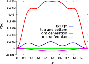
Figure 2: Contributions from the gauge bosons, the SM quarks, exotic and mirror fermion. The mirror fermion in this figure is 3 representation.

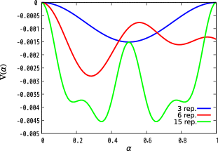
Figure 3: Effective potential of mirror fermions.

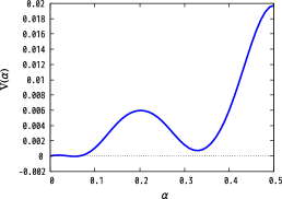
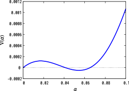
Figure 4: Higgs potential including 15 representation mirror fermions. The compactification scale $R^{-1}=1.82{\rm TeV}$ and the bulk mass for the mirror fermion $M=0.8{\rm TeV}$ are chosen.

5 Summary

In this paper, we proposed a new model of 5D $SU(3)\otimes U(1)_{X}$ GHU with a successful electroweak symmetry breaking and a realistic Higgs boson mass. In our model, the representations of the fermions are very simple, the $\bf 3,\bar{\bf 3}$ and $\overline{\bf 15}$ representations of $SU(3)$ gauge group. Since top quark is not embedded into the $\overline{\bf 15}$ representations, the anti-periodic boundary conditions can be imposed on $\overline{\bf 15}$. This reduced the number of the exotic massless fermions and the brane localized mass terms, which largely simplifies our analysis.

We have shown by calculating the 1-loop Higgs potential that a realistic electroweak symmetry breaking and the observed Higgs mass are realized in the case $R^{-1}=1.82\text{TeV},M=0.8\text{TeV}$. Note that a pair of additional $\overline{\bf 15}$ representations other than the SM fermions have been introduced to accomplish the above result. The fact that the observed Higgs mass cannot be obtained without extra fermions is consistent with the results in the third and the fifth papers in [6] and [10]. Furthermore, such extra fermions have been pointed out as the possible dark matter candidate [10]. We have also shown that the top and bottom quark masses are reproduced. As described in the main text, this is not a trivial issue since these masses are correlated through the mixing between the massless $SU(2)_{L}$ doublets from the up- and down-type sectors.

Finally, we give a comment on the relation to the SM-like property of the Higgs particle reported at LHC. Our Higgs potential has a periodicity with respect to the Higgs field because of the higher dimensional gauge symmetry. It is significantly different from the SM, however, the small expectation values are required to happen the electroweak symmetry breaking and to obtain a realistic Higgs mass. In that case, the differences are generically small and consistent with the current experimental data.

References

• [1] N. S. Manton, Nucl. Phys. B 158, 141 (1979); D. B. Fairlie, Phys. Lett. B 82, 97 (1979), J. Phys. G 5, L55 (1979); Y. Hosotani, Phys. Lett. B 126, 309 (1983), Phys. Lett. B 129, 193 (1983), Annals Phys.  190, 233 (1989).
• [2] H. Hatanaka, T. Inami and C. S. Lim, Mod. Phys. Lett. A 13, 2601 (1998).
• [3] I. Antoniadis, K. Benakli and M. Quiros, New J. Phys.  3, 20 (2001); G. von Gersdorff, N. Irges and M. Quiros, Nucl. Phys. B 635, 127 (2002); R. Contino, Y. Nomura and A. Pomarol, Nucl. Phys. B 671, 148 (2003); C. S. Lim, N. Maru and K. Hasegawa, J. Phys. Soc. Jap.  77, 074101 (2008); C. S. Lim, N. Maru and T. Miura, PTEP 2015 (2015) no.4, 043B02 K. Hasegawa, C. S. Lim and N. Maru, Phys. Lett. B 604, 133 (2004).
• [4] N. Maru and T. Yamashita, Nucl. Phys. B 754, 127 (2006); Y. Hosotani, N. Maru, K. Takenaga and T. Yamashita, Prog. Theor. Phys.  118, 1053 (2007).
• [5] C. S. Lim and N. Maru, Phys. Rev.  D 75, 115011 (2007).
• [6] N. Maru, Mod. Phys. Lett.  A 23, 2737 (2008); N. Maru and N. Okada, Phys. Rev.  D 77, 055010 (2008); Phys. Rev. D 87, no. 9, 095019 (2013); Phys. Rev. D 88, no. 3, 037701 (2013); arXiv:1310.3348 [hep-ph].
• [7] Y. Adachi, C. S. Lim and N. Maru, Phys. Rev.  D 76, 075009 (2007); Phys. Rev.  D 79, 075018 (2009); Phys. Rev.  D 80, 055025 (2009).
• [8] Y. Adachi, N. Kurahashi, C. S. Lim and N. Maru, JHEP 1011, 150 (2010); JHEP 1201, 047 (2012); Y. Adachi, N. Kurahashi, N. Maru and K. Tanabe, Phys. Rev. D 85, 096001 (2012); Y. Adachi, N. Kurahashi and N. Maru, arXiv:1404.4281 [hep-ph].
• [9] C. A. Scrucca, M. Serone and L. Silvestrini, Nucl. Phys. B 669, 128 (2003).
• [10] N. Maru, T. Miyaji, N. Okada and S. Okada, JHEP 1707 (2017) 048; N. Maru, N. Okada and S. Okada, Phys. Rev. D 96, no. 11, 115023 (2017).
• [11] Y. Adachi and N. Maru, PTEP 2016 (2016) no.7, 073B06.
• [12] C. Csaki, C. Grojean, J. Hubisz, Y. Shirman and J. Terning, Phys. Rev. D 70 (2004) 015012.
• [13] C. Patrignani et al. [Particle Data Group], Chin. Phys. C 40 (2016) no.10, 100001.