Monte Carlo Syntax Marginals for Exploring and Using
Dependency Parses

Abstract

Dependency parsing research, which has made significant gains in recent years, typically focuses on improving the accuracy of single-tree predictions. However, ambiguity is inherent to natural language syntax, and communicating such ambiguity is important for error analysis and better-informed downstream applications. In this work, we propose a transition sampling algorithm to sample from the full joint distribution of parse trees defined by a transition-based parsing model, and demonstrate the use of the samples in probabilistic dependency analysis. First, we define the new task of dependency path prediction, inferring syntactic substructures over part of a sentence, and provide the first analysis of performance on this task. Second, we demonstrate the usefulness of our Monte Carlo syntax marginal method for parser error analysis and calibration. Finally, we use this method to propagate parse uncertainty to two downstream information extraction applications: identifying persons killed by police and semantic role assignment.

[This paper appears in Proceedings of NAACL 2018]

1 Introduction

Dependency parsers typically predict a single tree for a sentence to be used in downstream applications, and most work on dependency parsers seeks to improve accuracy of such single-tree predictions. Despite tremendous gains in the last few decades of parsing research, accuracy is far from perfect—but perfect accuracy may be impossible since syntax models by themselves do not incorporate the discourse, pragmatic, or world knowledge necessary to resolve many ambiguities.

In fact, although relatively unexamined, substantial ambiguity already exists within commonly used discriminative probabilistic parsing models, which define a parse forest—a probability distribution $p(y\mid x)$ over possible dependency trees $y\in\mathcal{Y}(x)$ for an input sentence $x$.

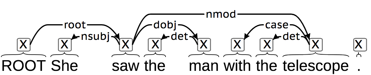
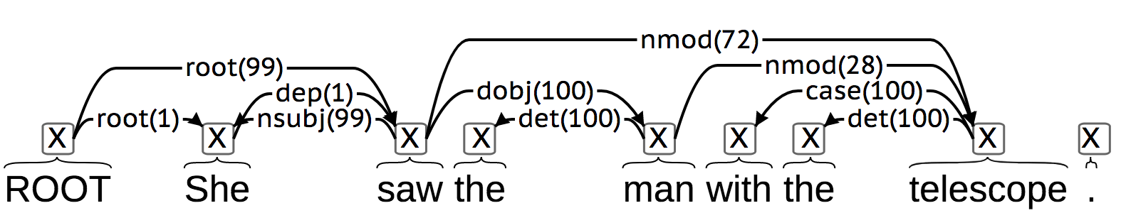
Figure 1: Example of a sentence with inherent ambiguity. Top: output from a greedy parser. Bottom: edge marginal probabilities from 100 samples in parentheses.

For example, the top of Figure 1 shows the predicted parse $y^{(greedy)}$ from such a parser (Chen and Manning, 2014), which resolves a prepositional (PP) attachment ambiguity in one manner; this prediction was selected by a standard greedy transition-based algorithm (§2.1). However, the bottom of Figure 1 shows marginal probabilities of individual (relation, governor, child) edges under this same model. These denote our estimated probabilities, across all possible parse structures, that a pair of words are connected with a particular relation (§2.4). For example, the two different PP attachment readings both exist within this parse forest with marginal probabilities

$$p(\text{ nmod}(\text{saw}_{2},\text{telescope}_{7})\mid x) =0.72$$ (1)

$$p(\text{ nmod}(\text{man}_{4},\text{telescope}_{7})\mid x) =0.28,$$ (2)

where (1) implies she used a telescope to see the man, and (2) implies she saw a man who had a telescope.

These types of irreducible syntactic ambiguities exist and should be taken into consideration when analyzing syntactic information; for instance, one could transmit multiple samples Finkel et al. (2006) or confidence scores Bunescu (2008) over ambiguous readings to downstream analysis components.

In this work, we introduce a simple transition sampling algorithm for transition-based dependency parsing (§2.2), which, by yielding exact samples from the full joint distribution over trees, makes it possible to infer probabilities of long-distance or other arbitrary structures over the parse distribution (§2.4). We implement transition sampling—a very simple change to pre-existing parsing software—and use it to demonstrate several applications of probabilistic dependency analysis:

• Motivated by how dependency parses are typically used in feature-based machine learning, we introduce a new parsing-related task—dependency path prediction. This task involves inference over variable length dependency paths, syntactic substructures over only parts of a sentence.

• To accomplish this task, we define a Monte Carlo syntax marginal inference method which exploits information across samples of the entire parse forest. It achieves higher accuracy predictions than a traditional greedy parsing algorithm, and allows tradeoffs between precision and recall (§4).

• We provide a quantitative measure of the model’s inherent uncertainty in the parse, whole-tree entropy, and show how it can be used for error analysis (§3).

• We demonstrate the method’s (surprisingly) reasonable calibration (§5).

• Finally, we demonstrate the utility of our method to propagate uncertainty to downstream applications. Our method improves performance for giving probabilistic semantics to a rule-based event extractor to identify civilians killed by police (§6), as well as semantic role assignment (§7).

2 Monte Carlo dependency analysis

2.1 Overview of transition-based dependency parsing

We examine the basic form of the Universal Dependencies formalism Nivre et al. (2016), where, for a sentence $x$ of length $N$, a possible dependency parse $y$ is a set of (relation, governorToken, childToken) edges, with a tree constraint that every token in the parse has exactly one governor—that is, for every token $w\in\{1..N\}$, there is exactly one triple $(r,g,w)\in y$ where it participates as a child. The governor is either one of the observed tokens, or a special ROOT vertex.

There exist a wide variety of approaches to machine learned, discriminative dependency parsing, which often define a probability distribution $p(y\mid x)$ over a domain of formally legal dependency parse trees $y\in\mathcal{Y}(x)$. We focus on transition-based dependency parsers Nivre (2003); Kübler et al. (2009), which (typically) use a stack-based automaton to process a sentence, incrementally building a set of edges. Transition-based parsers are very fast, have runtimes linear in sentence length, feature high performance (either state-of-the-art, or nearly so), and are easier to implement than other modeling paradigms (§2.5).

A probabilistic transition-based parser assumes the following stochastic process to generate a parse tree:

• Initialize state $S_{0}$ • For $n=1,2,\ldots$: (A) $a_{n}\sim p(a_{n}\mid S_{n-1})$ (B) $S_{n}:=\text{Update}(S_{n-1},a_{n})$ (C) Break if InEndState($S_{n}$)

Most state transition systems (Bohnet et al., 2016) use shift and reduce actions to sweep through tokens from left to right, pushing and popping them from a stack to create the edges that populate a new parse tree $y$. The action decision probability, $p(a_{next}\mid S_{current})$, is a softmax distribution over possible next actions. It can be parameterized by any probabilistic model, such as log-linear features of the sentence and current state Zhang and Nivre (2011), multilayer perceptrons Chen and Manning (2014), or recurrent neural networks Dyer et al. (2015); Kiperwasser and Goldberg (2016).

To predict a single parse tree on new data, a common inference method is greedy decoding, which runs a close variant of the above transition model as a deterministic automaton, replacing stochastic step (A) with a best-action decision, $a_{n}:=\arg\max_{a_{n}}p(a_{n}\mid S_{n-1})$. An inferred action sequence $a_{1:n}$ determines the resulting parse tree (edge set) $y$; the relationship can be denoted as $y(a_{1:n})$.

2.2 Transition sampling

In this work, we propose to analyze the full joint posterior $p(y\mid x)$, and use transition sampling, a very simple forward/ancestral sampling algorithm, to draw parse tree samples from that distribution. To parse a sentence, we run the automaton stochastically, sampling the action probability in step (A). This yields one action sequence $a_{1:n}$ from the full joint distribution of action sequences, and therefore a parse $y(a_{1:n})$ from the distribution of parses. We can obtain as many parse samples as desired by running the transition sampler $S$ times, yielding a collection (multiset) of parse structures $\{y^{(s)}\mid s\in\{1..S\}\}$, where each $y^{(s)}\sim p(y\mid x)$ is a full dependency parse tree. Runtime to draw one parse sample is very similar to the greedy algorithm’s runtime. We denote the set of unique parses in the sample $\tilde{\mathcal{Y}}(x)$.

We implement a transition sampler by modifying an implementation of Chen and Manning’s multilayer perceptron transition-based parser and use it for all subsequent experiments.

2.3 MC-MAP single parse prediction

One minor use of transition sampling is a method for predicting a single parse, by selecting the most probable (common) parse tree in the sample,

$$\hat{y}^{\text{MC-MAP}} =\arg\max_{y\in\tilde{\mathcal{Y}}}\ \tilde{p}(y\mid x)$$ (3)

$$=\arg\max_{y\in\tilde{\mathcal{Y}}}\ \frac{c(y)}{S}$$ (4)

where $\tilde{p}(y\mid x)$ denotes the Monte Carlo estimate of a parse’s probability, which is proportional to how many times it appears in the sample: $c(y)\equiv\sum_{s}^{S}1\{y=y^{(s)}\}$. Note that $\tilde{p}(y\mid x)$ correctly accounts for the case of an ambiguous transition system where multiple different action sequences can yield the same tree—i.e., $y(a_{1:n})$ is not one-to-one—since the transition sampler can sample the multiple different paths.

This “MC-MAP” method is asymptotically guaranteed to find the model’s most probable parse ($\arg\max_{y}p(y\mid x)$) given enough samples. By contrast, greedy decoding and beam search have no theoretical guarantees. MC-MAP’s disadvantage is that it may require a large number of samples, depending on the difference between the top parse’s probability compared to other parses in the domain.

2.4 Monte Carlo Syntax Marginal (MCSM) inference for structure queries

Beyond entire tree structures, parse posteriors also define marginal probabilities of particular events in them. Let $f(y)\rightarrow\{0,1\}$ be a boolean-valued structure query function of a parse tree—for example, whether the tree contains a particular edge:

$$f(y)=1\{\text{dobj(kill,Smith)}\in y\}$$

or more complicated structures, such as a length-2 dependency path:

$$f(y)=1\{\text{nsubj(kill},\text{cop})\land\text{dobj}(\text{kill},\text{Smith})\in y\}.$$

More precisely, these queries are typically formulated to check for edges between specific tokens, and may check tokens’ string forms.

Although $f(y)$ is a deterministic function, since the parsing model is uncertain of the correct parse, we find the marginal probability, or expectation, of a structure query by integrating out the posterior parse distribution—that is, the predicted probability that the parse has the property in question:

$$p(f(y)\mid x) =\sum_{y\in\mathcal{Y}(x)}f(y)\ p(y\mid x)$$ (5)

$$\approx\tilde{p}(f(y)\mid x) =\sum_{y\in\tilde{\mathcal{Y}}(x)}f(y)\frac{c(y)}{S}.$$ (6)

Eq. 5 is the expectation with regard to the model’s true probability distribution ($p$) over parses from the domain of all possible parse trees $\mathcal{Y}(x)$ for a sentence, while Eq. 6 is a Monte Carlo estimate of the query’s marginal probability—the fraction of parse tree samples where the structure query is true. We use this simple method for all inference in this work, though importance sampling Dyer et al. (2016), particle filters Buys and Blunsom (2015), or diverse k-best lists Zhang and McDonald (2014) could support more efficient inference in future work.

2.5 Probabilistic inference for dependencies: related work

Our transition sampling method aims to be an easy-to-implement algorithm for a highly performant class of dependency models, that conducts exact probabilistic inference for arbitrary structure queries in a reasonable amount of time. A wide range of alternative methods have been proposed for dependency inference that cover some, but perhaps not all, of these goals.

For transition-based parsing, beam search is a commonly used inference method that tries to look beyond a single structure. Beam search can be used to yield an approximate $K$-best list by taking resulting structures on the beam, though there are no theoretical guarantees about the result, and runtime is no better than the transition sampler. Finkel et al. (2006) further discuss tradeoffs between beam search and sampling, and find they give similar performance when propagating named entity recognition and PCFG parse information to downstream tasks.

Graph-based parsers are the major alternative modeling paradigm for dependency parsing; instead of a sequence of locally normalized decisions, they directly parameterize an entire tree’s globally normalized probability. Parse samples could be drawn from a graph-based model via Markov chain Monte Carlo Zhang et al. (2014), which is asymptotically correct, but may require a large amount of time to obtain non-autocorrelated parses. A range of methods address inference for specific queries in graph-based models—for example, edge marginals for edge-factored models via the matrix-tree theorem Koo et al. (2007), or approximate marginals with loopy belief propagation Smith and Eisner (2008). By contrast, our method is guaranteed to give correct marginal inferences for arbitrary, potentially long-distance, queries.

Given the strong performance of graph-based parsers in the single-structure prediction setting (e.g. Zeman et al. (2017); Dozat et al. (2017)), it may be worthwhile to further explore probabilistic inference for these models. For example, Niculae et al. (2018) present an inference algorithm for a graph-based parsing model that infers a weighted, sparse set of highly-probable parse trees, and they illustrate that it can infer syntactic ambiguities similar to Figure 1.

Dynamic programming for dependency parsing, as far as we are aware, has only been pursued for single-structure prediction (e.g. Huang and Sagae (2010)), but in principle could be generalized to calculate local structure query marginals via an inside-outside algorithm, or to sample entire structures through an inside-outside sampler (Eisner, 2016), which Finkel et al. (2006) use to propagate parse uncertainty for downstream analysis.

3 Exploratory error analysis via whole-tree entropy calculations

Sentence	Domain Size	Top 3 Freq.	Entropy
In Ramadi , there was a big demonstration .	3	[ 98, 1, 1 ]	0.112
US troops there clashed with guerrillas in a fight that left one Iraqi dead .	40	[ 33, 11, 6 ]	2.865
The sheikh in wheel - chair has been attacked with a F - 16 - launched bomb .	98	[ 2, 2, 1 ]	4.577

Table 1: Example sentences from the UD development set and summaries of their Monte Carlo parse distributions. Domain Size gives $|\tilde{\mathcal{Y}}_{100}|$, the number of unique parse structures in 100 samples. Top 3 Freq. gives the frequencies of the 3 most probable structures in $\tilde{\mathcal{Y}}_{100}$. Entropy is calculated according to Eq. 7; its upper bound is $\log(100)=4.605$.

In this section we directly explore the model’s intrinsic uncertainty, while §5 conducts a quantitative analysis of model uncertainty compared to gold standard structures. Parse samples are able to both pass on parse uncertainty and yield useful insights that typical error analysis approaches cannot. For a sentence $x$, we can calculate the whole-tree entropy, the model’s uncertainty of whole-tree parse frequencies in the samples:

$$H(p) =-\sum\limits_{y\in\mathcal{Y}(x)}p(y\mid x)\log p(y\mid x)$$

$$\approx H(\tilde{p}) =-\sum\limits_{y\in\tilde{\mathcal{Y}}(x)}\frac{c(y)}{S}\log\frac{c(y)}{S}.$$ (7)

Since this entropy estimate is only based on an $S$-sample approximation of $p$, it is upper bounded at $\log(S)$ in the case of a uniform MC distribution. Another intuitive measure of uncertainty is simply the number of unique parses, that is, the cardinality of the MC distribution’s domain $(|\tilde{\mathcal{Y}}|)$; this quantity is not informative for the true distribution $p$, but in the MC distribution it is intuitively upper bounded by $S$.

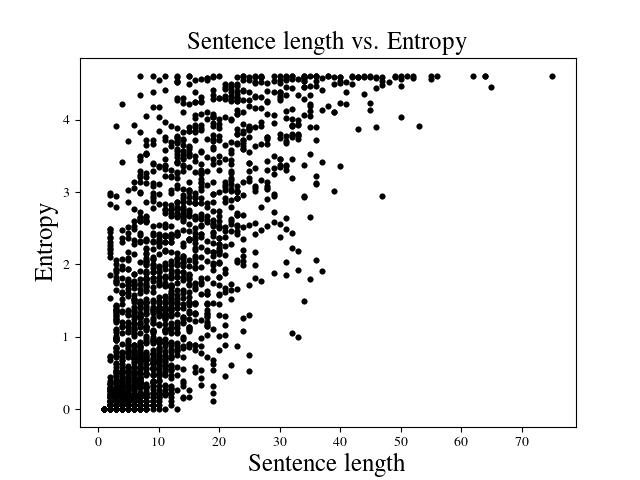
Figure 2: Length of sentences (in number of tokens in UD development set) against entropy (100 samples per sentence).

We run our dependency sampler on the 2002 sentences in the Universal Dependencies 1.3 English Treebank development set, generating 100 samples per sentence; Table 1 shows example sentences along with $|\tilde{\mathcal{Y}}|$ and entropy statistics for each sentence. We find that in general, as sentence length increases, so does the entropy of the parse distribution (Fig. 2). Moreover, we find that entropy is a useful diagnostic tool. For example, 7% of sentences in the UD development corpus with fewer than 15 tokens and $H(\tilde{p})\geq 2$ exhibit uncertainty around the role of ‘-’ (compare Sciences - principally biology and thought-provoking), and another 7% of such sentences exhibit uncertainty around ‘s’ (potentially representing a plural or a possessive).

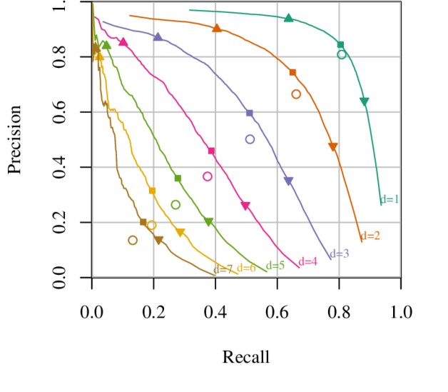
Path	Greedy	Marginal		MC-MAP
Len.	F1	Max F1	Thresh.	F1
1	$\bigcirc$ 0.808	$\blacksquare$ 0.824	0.45	0.807
2	$\bigcirc$ 0.663	$\blacksquare$ 0.694	0.44	0.660
3	$\bigcirc$ 0.506	$\blacksquare$ 0.550	0.34	0.501
4	$\bigcirc$ 0.370	$\blacksquare$ 0.420	0.28	0.363
5	$\bigcirc$ 0.268	$\blacksquare$ 0.314	0.25	0.262
6	$\bigcirc$ 0.192	$\blacksquare$ 0.241	0.25	0.188
7	$\bigcirc$ 0.134	$\blacksquare$ 0.182	0.17	0.131

$\blacktriangle$ Conf$\geq$0.9    $\blacktriangledown$ Conf$\geq$0.1

Figure 3: Precision-recall analysis against gold UD 1.3 English dev (§4.1) set for all dependency paths of lengths 1 to 7. Left: Each path length is a different color (1 in top-right, 7 in bottom-left), with greedy performance ($\bigcirc$) as well as the marginal path predictions’ PR curve, with points at confidence thresholds 0.9 ($\blacktriangle$), 0.1 ($\blacktriangledown$), and where F1 is highest ($\blacksquare$). Right: F1 for each method, as well as the confidence threshold for the marginal PR curve’s max-F1 point. For path length 1, Greedy and MC-MAP F1 are the same as labeled attachment score (LAS).

4 Monte Carlo Syntax Marginals for partial dependency parsing

Here we examine the utility of marginal inference for predicting parts of dependency parses, using the UD 1.3 Treebank’s English development set to evaluate.

4.1 Greedy decoding

Using its off-the-shelf pretrained model with greedy decoding, the CoreNLP parser achieves 80.8% labeled attachment score (LAS). LAS is equivalent to both the precision and recall of predicting (rel,gov,child) triples in the parse tree.

4.2 Minimum Bayes risk (MBR) decoding

A simple way to use marginal probabilities for parse prediction is to select, for each token, the governor and relation that has the highest marginal probability. This method gives a minimum Bayes risk (MBR) prediction of the parse, minimizing the model’s expected LAS with regards to local uncertainty; similar MBR methods have been shown to improve accuracy in tagging and constituent parsing (e.g. Goodman (1996); Petrov and Klein (2007)). This method yields 81.4% LAS, outperforming greedy parsing, though it may yield a graph that is not a tree.

4.3 Syntax marginal inference for dependency paths

An alternative view on dependency parsing is to consider what structures are needed for downstream applications. One commonly used parse substructure is the dependency path between two words, which is widely used in unsupervised lexical semantics (Lin and Pantel, 2001), distantly supervised lexical semantics (Snow et al., 2005), relation learning (Riedel et al., 2013), and supervised semantic role labeling (Hacioglu, 2004; Das et al., 2014), as well as applications in economics (Ghose et al., 2007), political science (O’Connor et al., 2013), biology (Fundel et al., 2006), and the humanities (Bamman et al., 2013, 2014).

In this work, we consider a dependency path to be a set of edges from the dependency parse; for example, a length-2 path $p=\{\text{nsubj}(3,1),\text{dobj}(3,4)\}$ connects tokens 1 and 4. Let $\mathcal{P}_{d}(y)$ be the set of all length-$d$ paths from a parse tree $y$. Figure 3’s “Greedy” table column displays the F-scores for the precision and recall of retrieving $\mathcal{P}_{d}(y^{(gold)})$ from the prediction $\mathcal{P}_{d}(y^{(greedy)})$ for a series of different path lengths. $\mathcal{P}_{1}$ gives individual edges, and thus is the same as LAS (80.8%). Longer length paths see a rapid decrease in performance; even length-2 paths are retrieved with only $\approx 66\%$ precision and recall. We are not aware of prior work that evaluates dependency parsing beyond single edge or whole sentence accuracy.

We define dependency path prediction as the task of predicting a set of dependency paths for a sentence; the paths do not necessarily have to come from the same tree, nor even be consistent with a single syntactic analysis. We approach this task with our Monte Carlo syntax marginal method, by predicting paths from the transition sampling parser. Here we treat each possible path as a structure query ($\S\ref{s:squery}$) and return all paths whose marginal probabilities are at least threshold $t$. Varying $t$ trades off precision and recall.

We apply this method to 100 samples per sentence in the UD treebank. When we take all length-1 paths that appear in every single sample (i.e., estimated marginal probability $1.0$), precision greatly increases to $0.969$, while recall drops to $0.317$ (the top-left point on Figure 3’s teal length-1 curve.) We can also accommodate applications which may prefer to have a higher recall: predicting all paths with at least $0.01$ probability results in $0.936$ recall (the bottom-right point on the curve in Figure 3).

This marginal path prediction method dominates the greedy parser: for length-1 paths, there are points on the marginal decoder’s PR curve that achieve both higher precision and recall than the greedy decoder, giving F1 of 82.4% when accepting all edges with marginal probability at least $0.45$. Furthermore, these advantages are more prominent for longer dependency paths. For example, for length-3 paths, the greedy parser only achieves 50.6% F1, while the marginal parser improves a bit to 55.0% F1; strikingly, it is possible to select high-confidence paths to get much higher 90.1% precision (at recall 11.6%, with confidence threshold $t=0.95$). Figure 3 also shows the precision/recall points on each curve for thresholds $t=0.9$ and $t=0.1$.

We also evaluated the MC-MAP single-parse prediction method (§2.3), which slightly, but consistently, underperforms the greedy decoder at all dependency lengths. More work is required to understand whether this is is an inference or modeling problem: for example, we may not have enough samples to reliably predict a high-probability parse; or, as some previous work finds in the context of beam search, the label bias phenomenon in this type of locally-normalized transition-based parser may cause it to assign higher probability to non-greedy analyses that in fact have lower linguistic quality Zhang and Nivre (2012); Andor et al. (2016).

5 Calibration

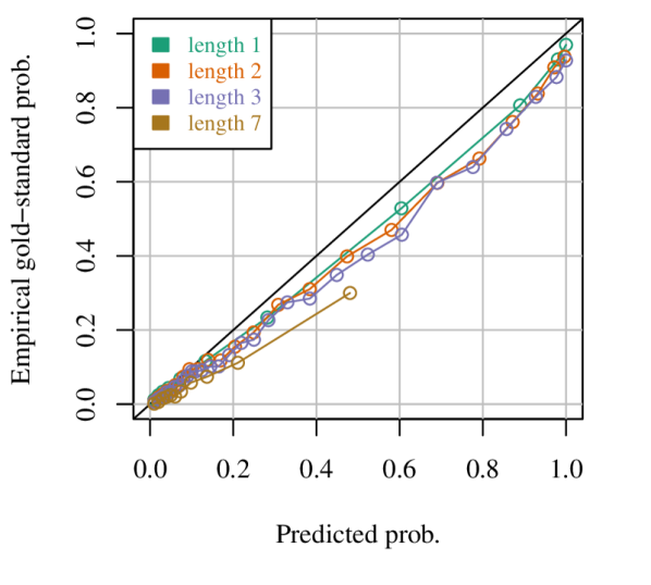
Figure 4: Calibration curves for marginal predictions for several path lengths. Predictions below the $y=x$ line indicate overconfidence. Points denote the average predicted probability versus empirical (gold) probability among predicted paths within each dynamically allocated bin.

The precision-recall analysis shows that the predicted marginal probabilities are meaningful in a ranking sense, but we can also ask whether they are meaningful in a sense of calibration: predictions are calibrated if, among all structures with predicted probability $q\pm\epsilon$, they exist in the gold parses with probability $q$. That is, predictions with confidence $q$ have precision $q$. If probabilities are calibrated, that implies expectations with regard to their distribution are unbiased, and may also justify intuitive interpretations of probabilities in exploratory analysis (§3). Calibration may also have implications for joint inference, EM, and active learning methods that use confidence scores and confidence-based expectations.

We apply Nguyen and O’Connor (2015)’s adaptive binning method to analyze the calibration of structure queries from an NLP system, by taking the domain of all seen length-$d$ paths from the 100 samples’ parse distribution for the treebank, grouping by ranges of predicted probabilities to have at least 5000 paths per bin, to ensure stability of the local precision estimate.

We find that probabilities are reasonably well calibrated, if slightly overconfident—Figure 4 shows the average predicted probability per bin, compared to how often these paths appear in the gold standard (local precision). For example, for edges (length-1 paths), predictions near 60% confidence (the average among predictions in range $[0.42,0.78]$) correspond to edges that are actually in the gold standard tree only 52.8% of the time. The middle confidence range has worse calibration error, and longer paths perform worse. Still, this level of calibration seems remarkably good, considering there was no attempt to re-calibrate predictions (Kuleshov and Liang, 2015) or to use a model that specifically parameterizes the energy of dependency paths (Smith and Eisner, 2008; Martins et al., 2010)—these predictions are simply a side effect of the overall joint model for incremental dependency parsing.

6 Probabilistic rule-based IE: classifying police fatalities

Supervised learning typically gives the most accurate information extraction or semantic parsing systems, but for many applications where training data is scarce, Chiticariu et al. (2013) argue that rule-based systems are useful and widespread in practice, despite their neglect in contemporary NLP research. Syntactic dependencies are a useful abstraction with which to write rule-based extractors, but they can be brittle due to errors in the parser. We propose to integrate over parse samples to infer a marginal probability of a rule match, increasing robustness and allowing for precision-recall tradeoffs.

6.1 Police killings victim extraction

We examine the task of extracting the list of names of persons killed by police from a test set of web news articles in Sept–Dec 2016. We use the dataset released by Keith et al. (2017), consisting of 24,550 named entities $e\in\mathcal{E}$ and sentences from noisy web news text extractions (that can be difficult to parse), each of which contains at least one $e$ (on average, 2.8 sentences/name) as well as keywords for both police and killing/shooting. The task is to classify whether a given name is a person who was killed by police, given 258 gold-standard names that have been verified by journalists.

6.2 Dependency rule exractor

Keith et al. present a baseline rule-based method that uses Li and Ji (2014)’s off-the-shelf RPI-JIE ACE event parser to extract (event type, agent, patient) tuples from sentences, and assigns $f_{\text{JIE}}(x_{i},e)=1$ iff the event type was a killing, the agent’s span included a police keyword, and the patient was the candidate entity $e$. An entity is classified as a victim if at least one sentence is classified as true, resulting in a 0.17 F1 score (as reported in previous work).

We define a similar syntactic dependency rule system using a dependency parse as input: our extractor $f(x,e,y)$ returns 1 iff the sentence has a killing keyword $k$, which both

1. has an agent token $a$ (defined as, governed by nsubj or nmod) which is a police keyword, or $a$ has a (amod or compound) modifier that is a police keyword; and,

2. has a patient token $p$ (defined as, governed by nsubjpass or dobj) contained in the candidate name $e$’s span.

Applying this $f(x,e,y)$ classifier to greedy parser output, it performs better than the RPI-JIE-based rules (Figure 5, right), perhaps because it is better customized for the particular task.

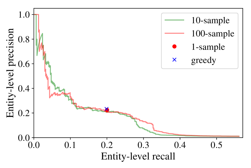
Method	F1
RPI-JIE	0.170
Greedy	0.215
1 samp.	0.212
10 samp.	0.219
100 samp.	0.222

Figure 5: Left: Rule-based entity precision and recall for police fatality victims, with greedy parsing and Monte Carlo inference. Right: F1 scores for RPI-JIE, Greedy, and 1-sample methods, and maximum F1 on PR curve for probabilistic (multiple sample) inference.

Treating $f$ as a structure query, we then use our Monte Carlo marginal inference (§2) method to calculate the probability of a rule match for each sentence—that is, the fraction of parse samples where $f(x,e,y^{(s)})$ is true—and infer the entity’s probability with the noisy-or formula (Craven and Kumlien, 1999; Keith et al., 2017). This gives soft classifications for entities.

6.3 Results

The Monte Carlo method achieves slightly higher F1 scores once there are at least 10 samples (Fig. 5, right). More interestingly, the soft entity-level classifications also allow for precision-recall tradeoffs (Fig. 5, left), which could be used to prioritize the time of human reviewers updating the victim database (filter to higher precision), or help ensure victims are not missed (with higher recall). We found the sampling method retrieved several true-positive entities where only a single sentence had a non-zero rule prediction at probability 0.01—that is, the rule was only matched in one of 100 sampled parses. Since current practitioners are already manually reviewing millions of news articles to create police fatality victim databases, the ability to filter to high recall—even with low precision—may be useful to help ensure victims are not missed.

6.4 Supervised learning

Sampling also slightly improves supervised learning for this problem. We modify Keith et al.’s logistic regression model based on a dependency path feature vector $f(x_{i},y)$, instead creating feature vectors that average over multiple parse samples ($E_{\tilde{p}(y)}[f(x_{i},y)]$) at both train and test time. With the greedy parser, the model results in 0.229 F1; using 100 samples slightly improves performance to 0.234 F1.

7 Semantic role assignment

Semantic role labeling (SRL), the task to predict argument structures Gildea and Jurafsky (2002), is tightly tied to syntax, and previous work has found it beneficial to conduct it with joint inference with constituency parsing, such as with top-$k$ parse trees Toutanova et al. (2008) or parse tree samples Finkel et al. (2006). Since §4 shows that Monte Carlo marginalization improves dependency edge prediction, we hypothesize dependency sampling could improve SRL as well.

SRL includes both identifying argument spans, and assigning spans to specific semantic role labels (argument types). We focus on just the second task of semantic role assignment: assuming argument spans are given, to predict the labels. We experiment with English OntoNotes v5.0 annotations Weischedel et al. (2013) according to the CoNLL 2012 test split Pradhan et al. (2013). We focus only on predicting among the five core arguments (Arg0 through Arg4) and ignore spans with gold-standard adjunct or reference labels. We fit a separate model for each predicate among the 2,160 predicates that occur at least once in both the training and test sets (115,811 and 12,216 sentences respectively).

Our semantic model of label $z_{t}\in\{A0..A4\}$ for argument head token $t$ and predicate token $p$, $p_{\text{sem}}(z_{t}\mid p,y)$, is simply the conditional probability of the label, conditioned on $y$’s edge between $t$ and $p$ if one exists. (If they are not directly connected, the model instead conditions on a ‘no edge’ feature.) Probabilities are maximum likelihood estimates from the training data’s (predicate, argument label, path) counts, from either greedy parses, or averaged among parse samples. To predict at test time, the greedy parsing model simply uses $p(z_{t}\mid p,y^{(greedy)})$. The Monte Carlo model, by contrast, treats it as a directed joint model and marginalizes over syntactic analyses:

$$p_{MC}(z_{t}\mid p,x)=\sum_{y\in\tilde{\mathcal{Y}}(x)}p_{\text{sem}}(z_{t}\mid p,y)\ \tilde{p}_{\text{syn}}(y\mid x).$$

The baseline accuracy of predicting the predicate’s most common training-time argument label yields 0.393 accuracy, and the greedy parser performs at 0.496. The Monte Carlo method (with 100 samples) improves accuracy to 0.529 (Table 2). Dependency samples’ usefulness in this limited case suggests they may help systems that use dependency parses more broadly for SRL Hacioglu (2004); Das et al. (2014).

Method	Accuracy
Baseline (most common)	0.393
Greedy	0.496
MCSM method, 100-samples	0.529

Table 2: Semantic role assignment accuracy on English OntoNotes v5.0. The baseline is for each unique predicate, predict the argument that was seen the most at training time.

8 Conclusion

In this work, we introduce a straightforward algorithm for sampling from the full joint distribution of a transition-based dependency parser. We explore using these parse samples to discover both parsing error and structural ambiguities. Moreover, we find that our Monte Carlo syntax marginal method not only dominates the greedy method for dependency path prediction (especially for longer paths), but also allows for control of precision-recall tradeoffs. Propagating dependency uncertainty can potentially help a wide variety of semantic analysis and information extraction tasks.

References

- Andor et al. (2016) Daniel Andor, Chris Alberti, David Weiss, Aliaksei Severyn, Alessandro Presta, Kuzman Ganchev, Slav Petrov, and Michael Collins. 2016. Globally normalized transition-based neural networks. In Proceedings of ACL.
- Bamman et al. (2013) David Bamman, Brendan O’Connor, and Noah A. Smith. 2013. Learning latent personas of film characters. In Proceedings of ACL.
- Bamman et al. (2014) David Bamman, Ted Underwood, and Noah A. Smith. 2014. A Bayesian mixed effects model of literary character. In Proceedings of ACL.
- Barber (2012) David Barber. 2012. Bayesian Reasoning and Machine Learning. Cambridge University Press.
- Bennett (2000) Paul N. Bennett. 2000. Assessing the calibration of naive Bayes’ posterior estimates. Technical report, Carnegie Mellon University.
- Bohnet et al. (2016) Bernd Bohnet, Ryan McDonald, Emily Pitler, and Ji Ma. 2016. Generalized transition-based dependency parsing via control parameters. In Proceedings of ACL. http://www.aclweb.org/anthology/P16-1015.
- Bunescu (2008) Razvan Bunescu. 2008. Learning with probabilistic features for improved pipeline models. In Proceedings of EMNLP. http://www.aclweb.org/anthology/D08-1070.
- Buys and Blunsom (2015) Jan Buys and Phil Blunsom. 2015. A bayesian model for generative transition-based dependency parsing. In Proceedings of the Third International Conference on Dependency Linguistics (Depling 2015). Uppsala, Sweden. http://www.aclweb.org/anthology/W15-2108.
- Chen and Manning (2014) Danqi Chen and Christopher Manning. 2014. A fast and accurate dependency parser using neural networks. In Proceedings of EMNLP. http://www.aclweb.org/anthology/D14-1082.
- Chiticariu et al. (2013) Laura Chiticariu, Yunyao Li, and Frederick R. Reiss. 2013. Rule-based information extraction is dead! long live rule-based information extraction systems! In Proceedings of EMNLP. http://www.aclweb.org/anthology/D13-1079.
- Craven and Kumlien (1999) Mark Craven and Johan Kumlien. 1999. Constructing biological knowledge bases by extracting information from text sources. In ISMB. pages 77–86.
- Das et al. (2014) Dipanjan Das, Desai Chen, Andre F. T. Martins, Nathan Schneider, and Noah A. Smith. 2014. Frame-semantic parsing. Computational Linguistics .
- Dozat et al. (2017) Timothy Dozat, Peng Qi, and Christopher D Manning. 2017. Stanford’s graph-based neural dependency parser at the conll 2017 shared task. Proceedings of the CoNLL 2017 Shared Task: Multilingual Parsing from Raw Text to Universal Dependencies pages 20–30.
- Dyer et al. (2015) Chris Dyer, Miguel Ballesteros, Wang Ling, Austin Matthews, and Noah A. Smith. 2015. Transition-based dependency parsing with stack long short-term memory. In Proceedings of ACL. http://www.aclweb.org/anthology/P15-1033.
- Dyer et al. (2016) Chris Dyer, Adhiguna Kuncoro, Miguel Ballesteros, and Noah A. Smith. 2016. Recurrent neural network grammars. In Proceedings of NAACL. http://www.aclweb.org/anthology/N16-1024.
- Efron (2010) Bradley Efron. 2010. Large-Scale Inference: Empirical Bayes Methods for Estimation, Testing, and Prediction. Cambridge University Press, 1st edition.
- Eisner (2016) Jason Eisner. 2016. Inside-outside and forward-backward algorithms are just backprop (tutorial paper). In Proceedings of the Workshop on Structured Prediction for NLP. Association for Computational Linguistics, Austin, TX, pages 1–17. http://aclweb.org/anthology/W16-5901.
- Finkel et al. (2006) Jenny Rose Finkel, Christopher D. Manning, and Andrew Y. Ng. 2006. Solving the problem of cascading errors: Approximate Bayesian inference for linguistic annotation pipelines. In Proceedings of EMNLP.
- Fundel et al. (2006) Katrin Fundel, Robert Küffner, and Ralf Zimmer. 2006. Relex—relation extraction using dependency parse trees. Bioinformatics 23(3):365–371.
- Ghose et al. (2007) Anindya Ghose, Panagiotis Ipeirotis, and Arun Sundararajan. 2007. Opinion mining using econometrics: A case study on reputation systems. In Proceedings of ACL. Prague, Czech Republic. http://www.aclweb.org/anthology/P07-1053.
- Gildea and Jurafsky (2002) Daniel Gildea and Daniel Jurafsky. 2002. Automatic labeling of semantic roles. Computational linguistics 28(3):245–288.
- Goodman (1996) Joshua Goodman. 1996. Parsing algorithms and metrics. In Proceedings of ACL. https://doi.org/10.3115/981863.981887.
- Hacioglu (2004) Kadri Hacioglu. 2004. Semantic role labeling using dependency trees. In Proceedings of the 20th international conference on Computational Linguistics. Association for Computational Linguistics.
- Huang and Sagae (2010) Liang Huang and Kenji Sagae. 2010. Dynamic programming for linear-time incremental parsing. In Proceedings of the 48th Annual Meeting of the Association for Computational Linguistics. Association for Computational Linguistics, Uppsala, Sweden, pages 1077–1086. http://www.aclweb.org/anthology/P10-1110.
- Keith et al. (2017) Katherine Keith, Abram Handler, Michael Pinkham, Cara Magliozzi, Joshua McDuffie, and Brendan O’Connor. 2017. Identifying civilians killed by police with distantly supervised entity-event extraction. In Proceedings of EMNLP.
- Kiperwasser and Goldberg (2016) Eliyahu Kiperwasser and Yoav Goldberg. 2016. Simple and accurate dependency parsing using bidirectional LSTM feature representations. Transactions of ACL .
- Koo et al. (2007) Terry Koo, Amir Globerson, Xavier Carreras, and Michael Collins. 2007. Structured prediction models via the matrix-tree theorem. In Proceedings of EMNLP. http://www.aclweb.org/anthology/D/D07/D07-1015.
- Kübler et al. (2009) Sandra Kübler, Ryan McDonald, and Joakim Nivre. 2009. Dependency parsing. Synthesis Lectures on Human Language Technologies .
- Kuleshov and Liang (2015) Volodymyr Kuleshov and Percy S. Liang. 2015. Calibrated structured prediction. In Advances in Neural Information Processing Systems.
- Li and Ji (2014) Qi Li and Heng Ji. 2014. Incremental joint extraction of entity mentions and relations. In Proceedings of ACL. pages 402–412.
- Lin and Pantel (2001) Dekang Lin and Patrick Pantel. 2001. DIRT – discovery of inference rules from text. In Proceedings of KDD.
- Martins et al. (2010) Andre Martins, Noah Smith, Eric Xing, Pedro Aguiar, and Mario Figueiredo. 2010. Turbo parsers: Dependency parsing by approximate variational inference. In Proceedings of EMNLP. http://www.aclweb.org/anthology/D10-1004.
- Nguyen and O’Connor (2015) Khanh Nguyen and Brendan O’Connor. 2015. Posterior calibration and exploratory analysis for natural language processing models. In Proceedings of EMNLP. http://aclweb.org/anthology/D15-1182.
- Niculae et al. (2018) Vlad Niculae, André FT Martins, Mathieu Blondel, and Claire Cardie. 2018. SparseMAP: Differentiable sparse structured inference. arXiv preprint arXiv:1802.04223 .
- Niculescu-Mizil and Caruana (2005) Alexandru Niculescu-Mizil and Rich Caruana. 2005. Predicting good probabilities with supervised learning. In Proceedings of ICML.
- Nivre (2003) Joakim Nivre. 2003. An efficient algorithm for projective dependency parsing. In Proceedings of the 8th International Workshop on Parsing Technologies (IWPT).
- Nivre et al. (2016) Joakim Nivre, Marie-Catherine de Marneffe, Filip Ginter, Yoav Goldberg, Jan Hajic, Christopher D Manning, Ryan McDonald, Slav Petrov, Sampo Pyysalo, Natalia Silveira, Reut Tsarfaty, and Daniel Zeman. 2016. Universal dependencies v1: A multilingual treebank collection. In Proceedings of LREC.
- O’Connor et al. (2013) Brendan O’Connor, Brandon Stewart, and Noah A. Smith. 2013. Learning to extract international relations from political context. In Proceedings of ACL.
- Petrov and Klein (2007) Slav Petrov and Dan Klein. 2007. Improved inference for unlexicalized parsing. In Proceedings of NAACL HLT 2007.
- Pradhan et al. (2013) Sameer Pradhan, Alessandro Moschitti, Nianwen Xue, Hwee Tou Ng, Anders Björkelund, Olga Uryupina, Yuchen Zhang, and Zhi Zhong. 2013. Towards robust linguistic analysis using ontonotes. In CoNLL. pages 143–152.
- Riedel et al. (2013) Sebastian Riedel, Limin Yao, Andrew McCallum, and Benjamin M. Marlin. 2013. Relation extraction with matrix factorization and universal schemas. In Proceedings of NAACL. Atlanta, Georgia. http://www.aclweb.org/anthology/N13-1008.
- Smith and Eisner (2008) David Smith and Jason Eisner. 2008. Dependency parsing by belief propagation. In Proceedings of EMNLP. http://www.aclweb.org/anthology/D08-1016.
- Smith and Eisner (2007) David A. Smith and Jason Eisner. 2007. Bootstrapping feature-rich dependency parsers with entropic priors. In Proceedings of EMNLP. http://www.aclweb.org/anthology/D/D07/D07-1070.
- Snow et al. (2005) Rion Snow, Dan. Jurafsky, and Andrew Y. Ng. 2005. Learning syntactic patterns for automatic hypernym discovery. In Advances in Neural Information Processing Systems.
- Toutanova et al. (2008) Kristina Toutanova, Aria Haghighi, and Christopher D. Manning. 2008. A global joint model for semantic role labeling. Computational Linguistics 34(2):161–191.
- Weischedel et al. (2013) Ralph Weischedel, Martha Palmer, Mitchell Marcus, Eduard Hovy, Sameer Pradhan, Lance Ramshaw, Nianwen Xue, Ann Taylor, Jeff Kaufman, Michelle Franchini, et al. 2013. Ontonotes release 5.0 LDC2013T19. Linguistic Data Consortium, Philadelphia, PA .
- Zeman et al. (2017) Daniel Zeman, Martin Popel, Milan Straka, Jan Hajic, Joakim Nivre, Filip Ginter, Juhani Luotolahti, Sampo Pyysalo, Slav Petrov, Martin Potthast, Francis Tyers, Elena Badmaeva, Memduh Gokirmak, Anna Nedoluzhko, Silvie Cinkova, Jan Hajic jr., Jaroslava Hlavacova, Václava Kettnerová, Zdenka Uresova, Jenna Kanerva, Stina Ojala, Anna Missilä, Christopher D. Manning, Sebastian Schuster, Siva Reddy, Dima Taji, Nizar Habash, Herman Leung, Marie-Catherine de Marneffe, Manuela Sanguinetti, Maria Simi, Hiroshi Kanayama, Valeria dePaiva, Kira Droganova, Héctor Martínez Alonso, Çağrı Çöltekin, Umut Sulubacak, Hans Uszkoreit, Vivien Macketanz, Aljoscha Burchardt, Kim Harris, Katrin Marheinecke, Georg Rehm, Tolga Kayadelen, Mohammed Attia, Ali Elkahky, Zhuoran Yu, Emily Pitler, Saran Lertpradit, Michael Mandl, Jesse Kirchner, Hector Fernandez Alcalde, Jana Strnadová, Esha Banerjee, Ruli Manurung, Antonio Stella, Atsuko Shimada, Sookyoung Kwak, Gustavo Mendonca, Tatiana Lando, Rattima Nitisaroj, and Josie Li. 2017. Conll 2017 shared task: Multilingual parsing from raw text to universal dependencies. In Proceedings of the CoNLL 2017 Shared Task: Multilingual Parsing from Raw Text to Universal Dependencies. Association for Computational Linguistics, Vancouver, Canada, pages 1–19. http://www.aclweb.org/anthology/K17-3001.
- Zhang and McDonald (2014) Hao Zhang and Ryan McDonald. 2014. Enforcing structural diversity in cube-pruned dependency parsing. In Proceedings of ACL. http://www.aclweb.org/anthology/P14-2107.
- Zhang et al. (2014) Yuan Zhang, Tao Lei, Regina Barzilay, and Tommi Jaakkola. 2014. Greed is good if randomized: New inference for dependency parsing. In Proceedings of EMNLP. Doha, Qatar. http://www.aclweb.org/anthology/D14-1109.
- Zhang and Nivre (2011) Yue Zhang and Joakim Nivre. 2011. Transition-based dependency parsing with rich non-local features. In Proceedings of ACL. http://www.aclweb.org/anthology/P11-2033.
- Zhang and Nivre (2012) Yue Zhang and Joakim Nivre. 2012. Analyzing the effect of global learning and beam-search on transition-based dependency parsing. In Proceedings of COLING. http://www.aclweb.org/anthology/C12-2136.