A Complete Census of Luminous Stellar Variability on Day to Decade Timescales
Abstract
Stellar photometric variability offers a novel probe of the interior structure and evolutionary state of stars. Here we present a census of stellar variability on day to decade timescales across the color-magnitude diagram for 73,000 stars brighter than in the Whirlpool Galaxy (M51). Our Cycle 24 HST program acquired and band images over 34 epochs spanning one year with pseudo-random cadences enabling sensitivity to periods from days to months. We supplement these data with archival and band HST data obtained in 1995 and 2005, providing sensitivity to variability on decade timescales. At least 50% of stars brighter than show strong evidence for variability within our Cycle 24 data; amongst stars with the variability fraction rises to %. Large amplitude variability ( mag) on decade timescales is restricted to red supergiants and very luminous blue stars. Both populations display fairly smooth variability on month-year timescales. The Cepheid instability strip is clearly visible in our data, although the variability fraction within this region never exceeds %. The location of variable stars across the color magnitude diagram broadly agrees with theoretical sources of variability, including the instability strip, red supergiant pulsational instabilities, long-period fundamental mode pulsations, and radiation-dominated envelopes in massive stars. Our data can be used to place stringent constraints on the precise onset of these various instabilities and their lifetimes and growth rates.
Subject headings:
stars: variables: general, Hertzsprung-Russell and colour-magnitude, galaxies: individual (NGC 5194)1. Introduction
Stellar variability is a powerful tool to study a variety of phenomena in the Universe, including stellar interiors (via asteroseismology), the final stages of massive stars (via eruptive behavior, e.g., Carinae), the cosmic distance ladder (via the “Leavitt Law”—the Cepheid period–luminosity relation), stellar masses and radii (via eclipsing binaries and period–luminosity relations of evolved stars), and the explosive behavior of novae and supernovae (see reviews in Eyer & Mowlavi, 2008; Catelan & Smith, 2015).
The timescales, regularity, and amplitudes of stellar variability span essentially the entire observable parameter space. Variability occurs on the shortest observed timescales (seconds to minutes in the case of helioseismology) and the longest probed timescales (the light curves for Car and P Cyg span years). Some variables show regular, well-defined periods over long timescales, while others have unpredictable irregular behavior, such as eruptions of luminous blue variables (LBVs), in addition to the more spectacular novae and supernovae. Finally, variability amplitudes range from the smallest detectable fluctuations (ppm; e.g., Borucki et al., 2010), to several magnitude fluctuations amongst the LBVs, red supergiants (RSGs), and Mira variables, to much larger amplitudes for the novae and supernovae.
Stellar variability can be driven by a variety of physical processes. The best understood on theoretical grounds are the excitation of unstable radial or non-radial modes, as encountered in asteroseismology, luminous pulsating red variables such as Miras and semi-regular variables (SRVs) (e.g., Wood, 1979), Cepheids, RV Tau stars, and many others. These stars tend to experience moderate amplitude variability in their physical properties and for these reasons the variability is rarely destructive to the star. On the other hand, large amplitude variability, such as occurs in RSGs and LBVs can alter and/or hasten the subsequent evolution of the star (Heger et al., 1997; Yoon & Cantiello, 2010; Owocki, 2015; Smith & Owocki, 2006; Smith, 2014). Evolution of very massive stars () is quite uncertain both because of limited observational samples and because the underlying physics is poorly understood. For example, the physical origin of the luminosity variation observed in LBVs is a mystery, although there are many possibilities including violent strange mode instabilities (Yadav & Glatzel, 2017), unstable turbulent convection (Smith & Arnett, 2014), binary star merger products (Smith & Arnett, 2014; Justham et al., 2014), and radiation-dominated stellar envelopes near the local Eddington limit (Paxton et al., 2013; Jiang et al., 2015). Progress is limited in part by the rarity of massive stars and the long timescales involved, both of which make it challenging to test models against observations.
There have been many surveys of stellar variability in the Local Group and beyond, dating back to the early part of the last century (e.g., Leavitt, 1908; Hubble & Sandage, 1953; Tammann & Sandage, 1968). Time domain surveys have particularly proliferated in the past twenty years, with the advent of fast, wide format imaging systems. Examples include MACHO (Alcock et al., 1997), ASAS (Pojmanski, 2002), OGLE (Udalski, 2003), Pan-STARRS1 (Chambers et al., 2016), PTF (Law et al., 2009), CRTS (Drake et al., 2014), and ASAS-SN (Jayasinghe et al., 2018).
From these surveys and other dedicated efforts, stellar variability has been studied in the Galaxy, the Small and Large Magellanic Clouds, M31 and M33, and other nearby galaxies (e.g., Rejkuba et al., 2003; Hartman et al., 2006; Massey et al., 2007, 2009; Kourniotis et al., 2014; Martin & Humphreys, 2017; Humphreys et al., 2017; Soraisam et al., 2018). The LMC and SMC have probably the most complete information about stellar variability, given their close distance, low reddening, and the long time coverage of the ongoing OGLE survey.
However, one of the shortcomings of studying variability in the Magellanic Clouds, and in other dwarf galaxies such as M33, is that they do not offer a complete view of the variability among the massive star population. This is due to the simple fact that such stars are rare in galaxies with low stellar masses and low star formation rates. For example, the variability study of M33 from Hartman et al. (2006) is limited to (), and the LMC catalog of Mira variables from Soszyński et al. (2009) runs out of stars by ().
The study of more massive galaxies with higher star-formation rates offers a more complete view of stellar variability among the most luminous, massive stars. The Milky Way itself is not ideal, since (i) massive stars lie in the plane and are therefore subject to high extinction, (ii) distances to luminous stars are not well-known, and (iii) it is challenging to monitor the entire sky. The Gaia satellite will make substantial progress in addressing (ii) and (iii), but extinction will still make it difficult to perform a complete census, and Gaia parallaxes become quite uncertain beyond kpc.
M31 mitigates some of these issues, and data from PTF have been used to study specific classes of variables and transients. For example, Soraisam et al. (2018) performed a census of pulsating red supergiants in M31, and Kasliwal et al. (2011) presented the discovery of several faint, fast-declining novae in M31 that could have been missed in previous nova surveys.
Here we complement these previous studies with an investigation of stellar variability amongst the luminous star population in M51 (the Whirlpool Galaxy, NGC 5194), an galaxy with a stellar mass of (Mentuch Cooper et al., 2012) and a star formation rate (SFR) of yr-1 (Calzetti et al., 2005) at a distance of Mpc (McQuinn et al., 2016). In addition to being a galaxy with a large population of massive stars, studying variability within M51 offers several other benefits: the stars are all at a common distance; the galaxy subtends a small angle on the sky, minimizing foreground contamination; Galactic extinction is low and fairly constant across the field; the galaxy is face-on, minimizing internal reddening.
Perhaps the most unique aspect of this work is that our stellar variability census of M51 is based entirely on data acquired by the Hubble Space Telescope (HST). The benefits of HST are many, including a relatively well-characterized, stable PSF compared to ground-based observations. The angular resolution (FWHM) is (depending on the filter), corresponding to pc at the distance of M51 and is comparable in spatial resolution to ground-based photometry of M31.
The rest of this paper is organized as follows. In Section 2 we describe the data and methods. Section 3 contains our results including a census of stellar variability on day-to-decade timescales. We conclude with a summary in Section 4. All magnitudes are on the Vega zeropoint system, and absolute magnitudes are computed assuming a true distance modulus of 29.67 and Galactic extinction of and . In all cases we quote and magnitudes in the HST ACS F606W and F814W filters and refer to them as and , respectively. In cases where data were originally obtained or tabulated in another filter (such as F555W or Bessell V) we have converted them to F606W.
2. Data & Methods
2.1. HST Imaging
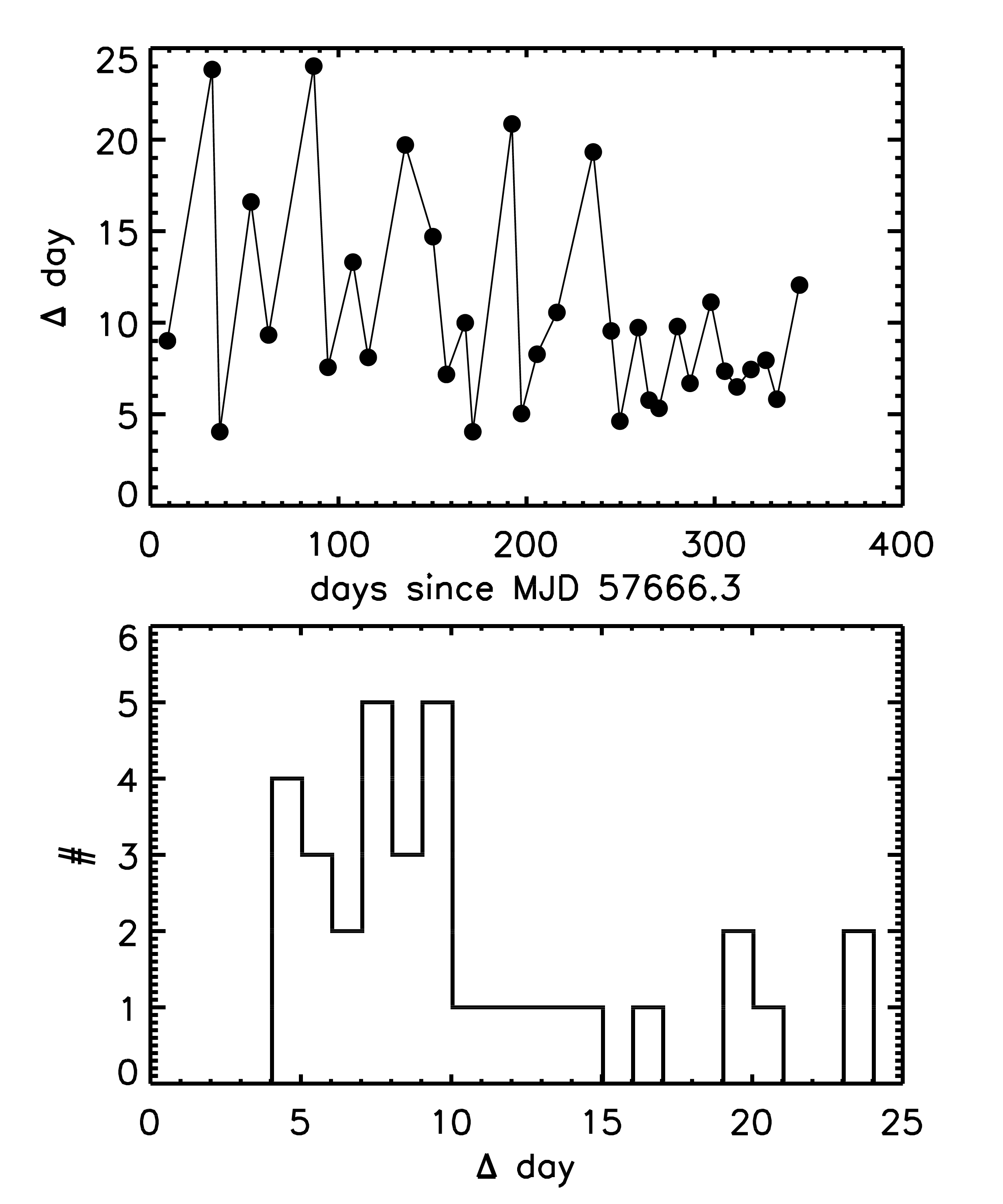
The main data presented in this paper are our Cycle 24 observations, collected in 34 epochs between Oct 2016 and Sept 2017 (Proposal ID 14704, PI Conroy). The primary purpose of these data is to measure the star formation history (SFH) of M51 via analysis of pixel light curves, a technique described in Conroy et al. (2015). The program required monitoring of M51 over a year, with a cadence determined by a desire to retain sensitivity to a wide range of periods (modulated by observatory constraints). The resulting cadence, shown in Figure 2, is pseudo-random with minimum/maximum separation between visits of 4/24 days. Data obtained in this way offer sensitivity to a wider range of periods than uniform sampling (see e.g., Freedman et al., 1994, , and Section 2.4).
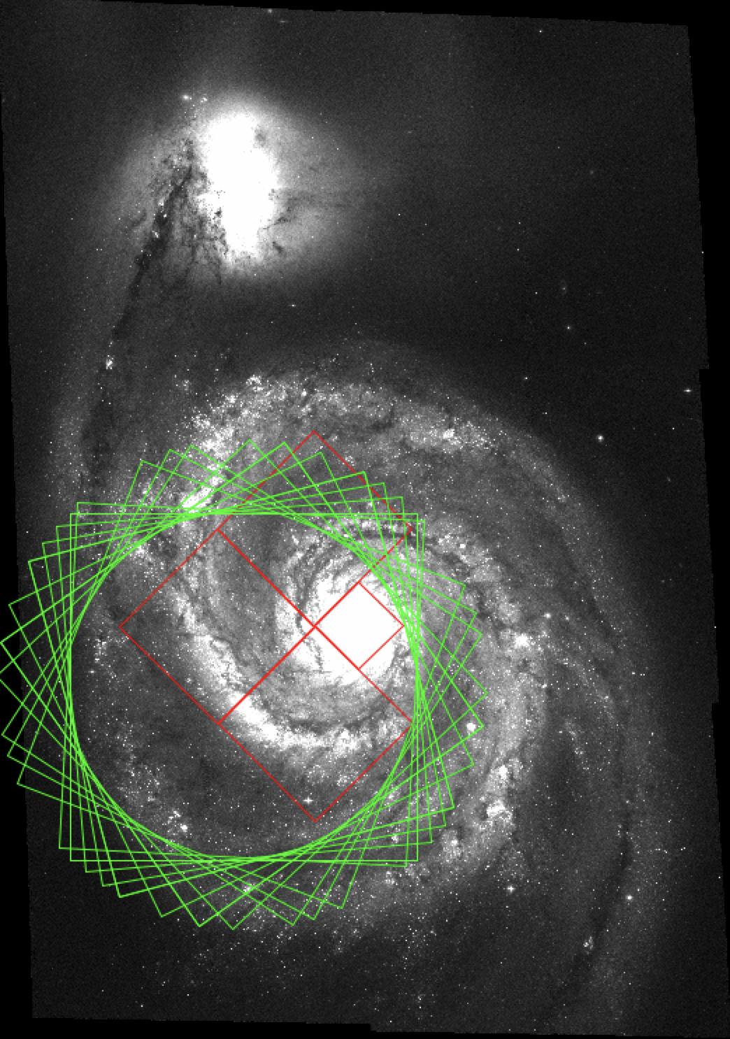
To monitor the same field over a full year required a variation of roll angle across the cycle (see Figure 1). We nonetheless required that each orientation have at least two visits, to ensure that the WFC3 parallel fields on the stellar halo would achieve sufficient depth to detect old red giants. The Cycle 24 data were obtained using the Advanced Camera for Surveys (ACS) with a standard four-point dither pattern, for a total of 2200 s per visit in each of the and . Only the ACS data are discussed in this paper; the parallel WFC3 data will be presented elsewhere.
To enable sensitivity to variability on timescales longer than 1 yr, we supplement these new data with older HST observations. The most important of these are the Cycle 13 data collected in January 2005 (Proposal ID 10452, PI Beckwith) as part of the Hubble Heritage project to obtain a six-pointing mosaic of the M51 system. A range of filters were obtained, but here we only use the and images, collected with s individual exposures in each filter per pointing.
Finally, we also analyze Cycle 4 data obtained in January 1995 (Proposal ID 5777, PI Kirshner) to follow up SN 1994I. These data were collected with WFPC2 in the and filters, with a single 600 s exposure per filter. Since only a single exposure was available, cosmic rays were removed via the L.A. Cosmic program (van Dokkum, 2001).
We note that many other observations have been made of M51 over the lifetime of ; we do not use these other data in this paper, typically because they only partially overlap with our primary fields, or are not taken in or -equivalent filters.
The footprints of all the data used are shown in Figure 1. Our Cycle 24 data contains 40% of the total band flux of M51 and the WFPC2 Cycle 4 data contains 60% of the band flux contained in our Cycle 24 data.
2.2. HRDs vs. CMDs
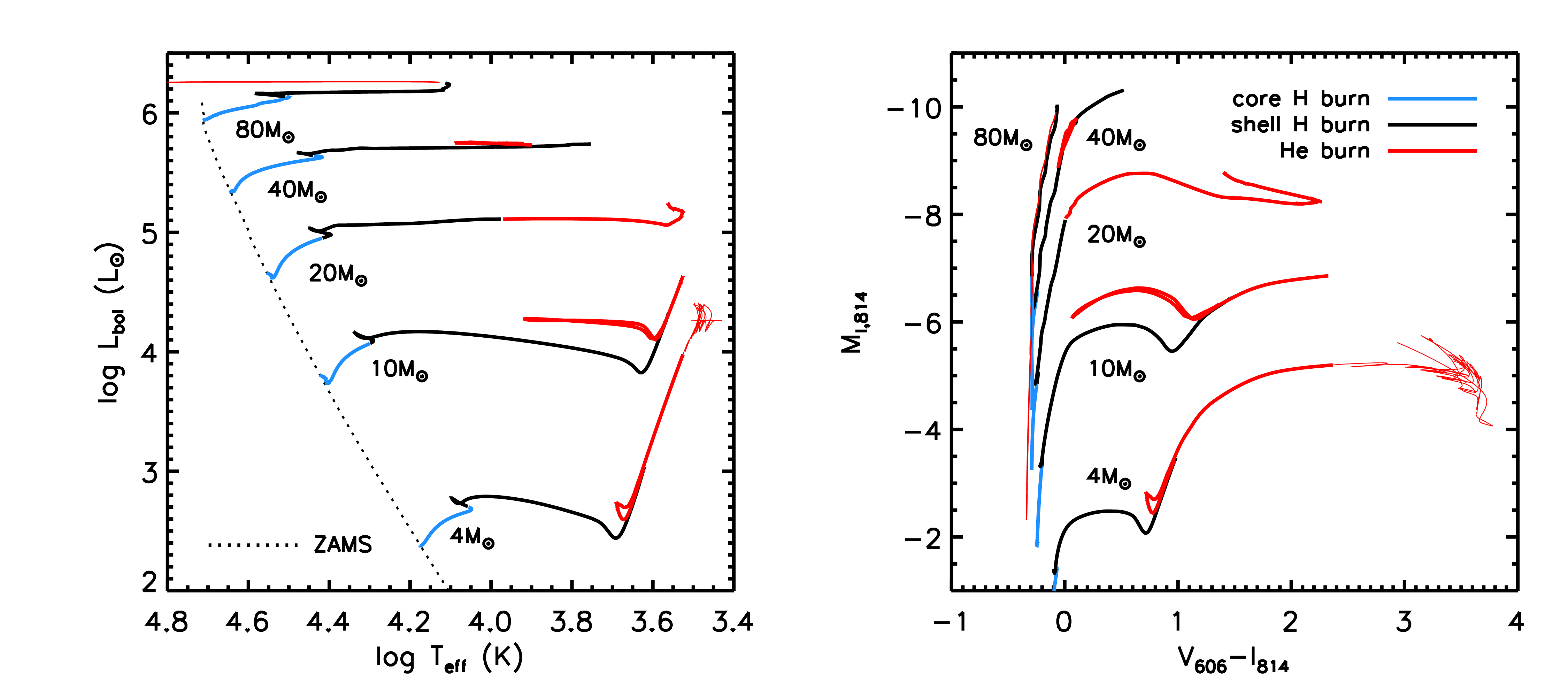
First we discuss the stars and the evolutionary phases that our program should be able to probe. In Figure 3 we show MIST (Choi et al., 2016) stellar evolutionary tracks for 4, 10, 20, 40, and starting at the zero-age main sequence (ZAMS, shown as a dotted line). The models are at solar metallicity. The tracks are color-coded by their evolutionary phase. The left panel shows the behavior in the HR diagram while the right panel shows the same models in the VI color-magnitude diagram (CMD).
The bolometric corrections for massive stars are substantial, especially for the hot stars. For example, a star evolves at approximately constant but brightens in by mag. Moreover, stars more massive than do not at any point exceed and indeed during the main sequence they are relatively faint in : an star has at the ZAMS. This leads us to an important point that will be relevant for interpreting the results in later sections: essentially every star brighter than is an evolved high-mass star.
2.3. Photometry
2.3.1 PSF photometry with DOLPHOT
We perform PSF photometry using the DOLPHOT software package (Dolphin, 2000). Briefly, DOLPHOT performs photometry by iteratively identifying stars, and simultaneously solves for the sky background and the magnitude of each star for an arbitrary number of aligned images in an arbitrary number of filters. DOLPHOT uses the TinyTim PSF models (Krist, 1995) and makes additional adjustments to the PSF using relatively bright, isolated stars. DOLPHOT also computes and applies aperture corrections. We supply to DOLPHOT CTE-corrected individual exposure-level images for the ACS data (flc files) and standard exposure-level images for the WFPC2 data (c0m files).
There are many parameters to set when running DOLPHOT. We adopt the parameters used for PSF photometry of M31 stars in the HST PHAT Survey (Dalcanton et al., 2012; Williams et al., 2014). We refer the interested reader to those papers, which describe extensive tests of the impact of various DOLPHOT parameters on the derived photometry.
After experimentation with a variety of analysis procedures, we decided to process the images in two DOLPHOT runs. The first contains the Cycle 24 data in both filters, and the second contains the Cycle 4, Cycle 13, and four visits from the Cycle 24 data to assist with the subsequent cross-matching between the two runs. This process ensured that stars that were well-detected in certain epochs/filters would have measured photometry in all available epochs/filters even in cases where the individual exposure S/N was low. The runs were split in two for computational efficiency (the Cycle 24 photometry took three weeks to complete). The catalogs were matched in pixel coordinates and we require an association of better than one pixel for a match, although in nearly all cases the match is within pixel. DOLPHOT measures and applies aperture corrections such that the reported photometry is within a radius of . We apply additional aperture corrections such that the final photometry is reported within an infinite aperture (see Bohlin, 2016).
DOLPHOT provides a number of parameters for each star, including a statistic of the goodness of fit (), several shape parameters (round and sharp), an “object type”, and a measure of the crowding. This last parameter is defined in magnitudes and quantifies how much brighter the star would be if nearby stars had not been fit simultaneously. Unsurprisingly, the crowding is strongly correlated between the and bands with a ( clipped) standard deviation of 0.15 mag. We require an object type (star), band crowding , band sharpness, sharp, and . We also require a final band S/N and detections in the band for least five epochs. We have also masked the central and regions around six bright foreground stars.
With these cuts our final catalog contains 320,000 stars, of which 73,000 are brighter than . 98% of stars brighter than have an identified band counterpart in the Cycle 24 data. The cross-matches between Cycle 24 -band and the archival band in the regions of overlap drop below 80% for and for the 2005 and 1995 data, respectively. This is mostly a reflection of the shorter exposure times in the archival data.
We comment briefly on possible confusion between star clusters and bright stars. The angular resolution (FWHM) of the () data is (), which at the distance of M51 corresponds to 3.33 (3.75) pc. For high S/N sources it is possible to separate stars from star clusters to a fraction of a resolution element. Based on HST analysis of star clusters in M31, Johnson et al. (2012) find sizes of the brighter clusters in the range of pc with very few below 1 pc. Our sample of stars is therefore unlikely to be contaminated by unresolved star clusters. However, unresolved similar-mass binaries will be a source of contamination in our catalog; such sources can only be identified with followup spectroscopic monitoring.
Corrections for Galactic extinction were applied to all photometry adopting the Schlafly & Finkbeiner (2011) reddening map. Specifically, we adopt , , . We convert all of the photometry to using and the bolometric correction tables distributed as part of the MIST project (Choi et al., 2016).
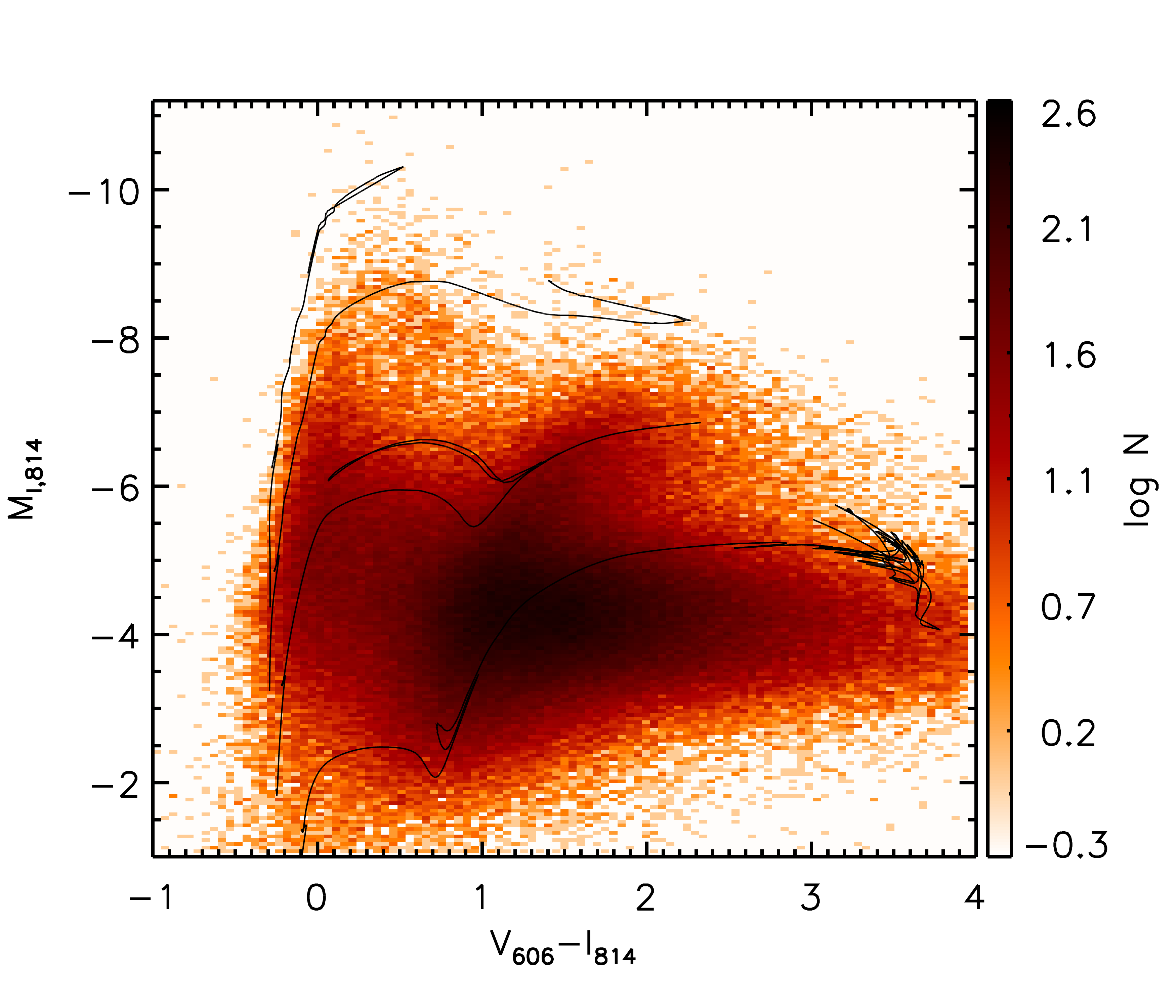
An overview CMD derived from the Cycle 24 data is shown in Figure 4. One clearly sees the locus of main sequence and blue core He burning stars at , the red core He burning stars (RSGs) occupying the diagonal sequence at and , and the asymptotic giant branch (AGB) stars at . incompleteness starts to become substantial at , especially for the redder stars.
2.3.2 Error budget
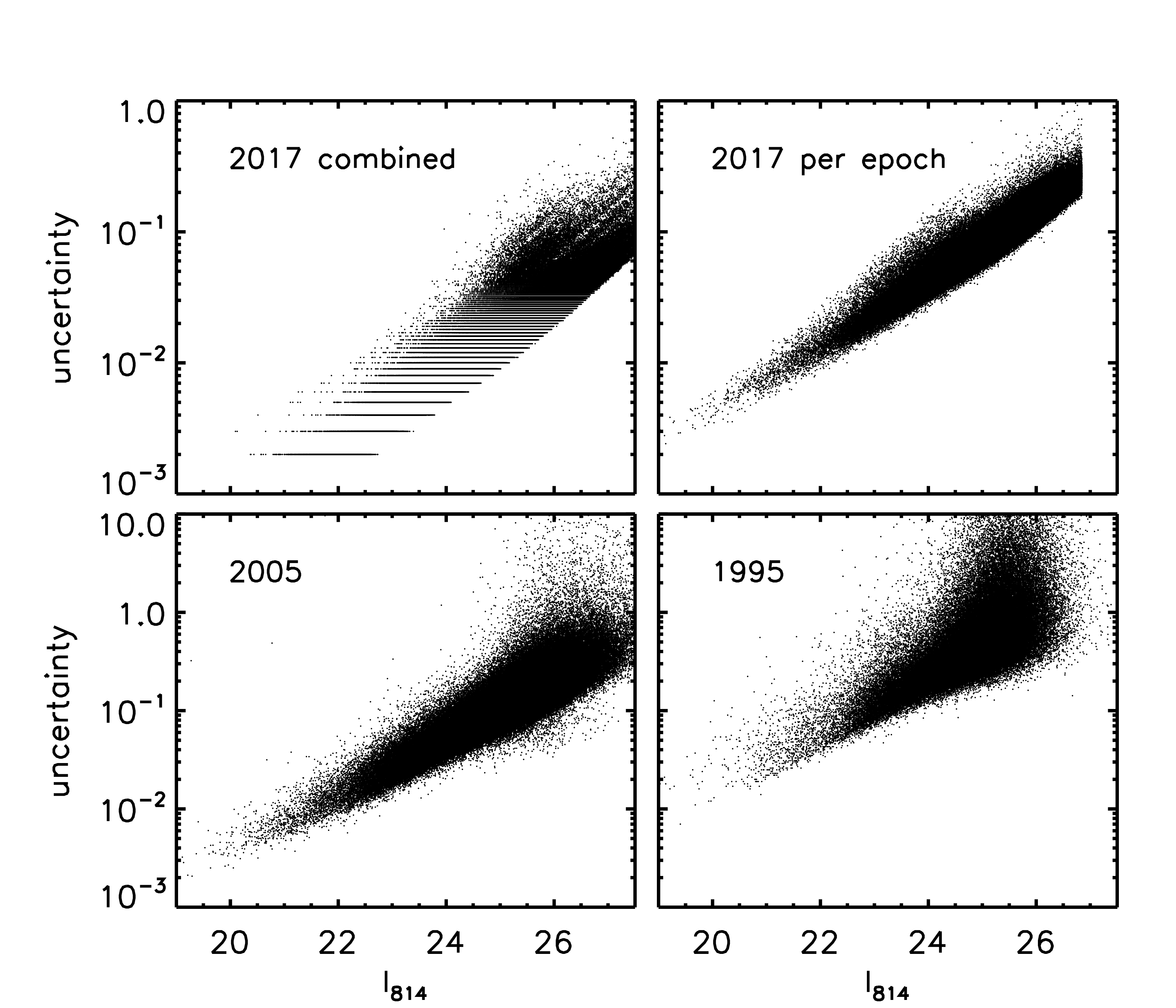
The error budget is critical for an accurate accounting of stellar variability. In Figure 5 we show the reported errors from DOLPHOT for the 1995, 2005, and 2017 (Cycle 24) data. For the latter we show two versions: the median (over the 34 visits) per epoch error, and the error on the final combined photometry. The uncertainties depend on several factors, including the photon noise, sky background level, and goodness of fit of the PSF model. Notice that the errors continue to decline toward brighter magnitudes.
As we will see in later sections, many bright stars have rms variations in their light curves at the mag level, so understanding additional sources of uncertainty not included in the default DOLPHOT output is important. To our knowledge all sub-percent-level variable star photometry has relied on differential photometry that employs non-variable stars as calibrators (e.g., Hartman et al., 2004; Nascimbeni et al., 2014; Jayasinghe et al., 2018). In our case this is not possible since we have reason to believe that the majority of bright stars are intrinsically variable. We therefore undertake a variety of tests of the absolute stability of the DOLPHOT PSF photometry, noting that previous work has found evidence for systematic uncertainties at the mag level (e.g., Dalcanton et al., 2012; Williams et al., 2014).
To test the DOLPHOT photometry we have selected a sample of bright, uncrowded stars with () and an band crowding parameter . We ran many permutations of the default DOLPHOT parameters including varying the sky subtraction model, the radius used to fit the PSF and the sky background, turning on/off the aperture corrections, and considering aperture photometry instead of PSF photometry. Nearly all of the changes had no discernable effect on the light curve rms, with the exception of aperture photometry with an aperture radius of 3 pixels. This choice of parameters resulted in a lower rms on average for . Larger and smaller values of did not change. This test suggests that the PSF model is insufficiently flexible to account for subtle changes in either time or location on the detector (see also Dalcanton et al., 2012; Williams et al., 2014). Unfortunately we cannot use aperture photometry for the bulk of our analysis because the vast majority of stars are in very crowded regions where simultaneous fitting of overlapping PSFs is essential for accurate photometry.
The large number of distinct orientations (17) allows us to perform a novel test of the reliability of the PSF photometry without relying on calibration from non-variable stars. If we consider a small region in the image plane, then as the orientation varies the stars at that position will also vary. Over the course of the full Cycle there will be 17 distinct populations of stars landing within a given image plane region. If the photometry were free of systematic errors, then the mean magnitude offset of the stars at each visit with respect to their individual mean magnitudes should be zero, i.e., should be zero where is the magnitude of the th star at the th orientation, is the mean magnitude of star across all visits, and is the number of stars at the th orientation. The sum is over all stars within a given small region in the image plane.
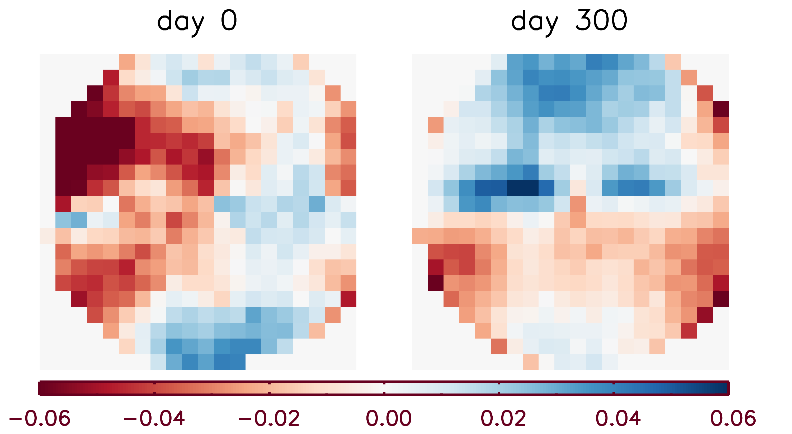
In practice we find that these mean magnitude offsets, or magnitude corrections, vary with time and with position in the image plane. We have computed magnitude correction maps in pixel regions across the image plane in both the and band. We then fit quadratic functions to the time-dependence of the corrections for regions containing stars (combined over all visits). These maps are shown in Figure 6 for the band at two epochs. The corrections range from to and vary in a systematic and generally smooth manner, although there are often sharp transitions across the chip gap (which runs horizontally through the center of these maps). We have applied these corrections to all our photometry and find that for these corrections result on average in smaller values. For values outside this range there is little change. As a final measure we add a systematic error of 0.02 mag to the quoted DOLPHOT uncertainties to capture residual issues at this low level.
The apparent time variation in the magnitude corrections may be due to some subtle underlying systematic, such as residual CTE effects combined with unmodeled variation in the point spread function. With very careful cosmic ray removal and large-aperture photometry of individual bright stars we were able to reduce the variation to after correcting for residual correlations in the image plane, but this methodology cannot be applied ”in bulk” or for crowded regions. Even though we have not been able to pinpoint the source of the variation, we stress that a) these same patterns are seen in previous studies, in particular PHAT (Dalcanton et al., 2012) and b) we can correct for them even if we do not understand the source. We also note that our main conclusions are not sensitive to these corrections, although they do affect the fractions of variable stars in the bin of lowest variability ( mag).
A common technique for assessing the quality of the DOLPHOT photometry is the use of artificial star tests (e.g., Dalcanton et al., 2012; Williams et al., 2014). The general idea is to inject stars with known fluxes into the image and to photometer those stars as usual with DOLPHOT to test how well the fluxes can be recovered as a function of magnitude and local stellar density. We stress that the injection of artificial stars only tests some of the possible sources of systematic uncertainties. For example, artificial stars are injected with the same model PSF used in the fitting, so this test cannot assess the systematic uncertainty associated with possible PSF mis-match.
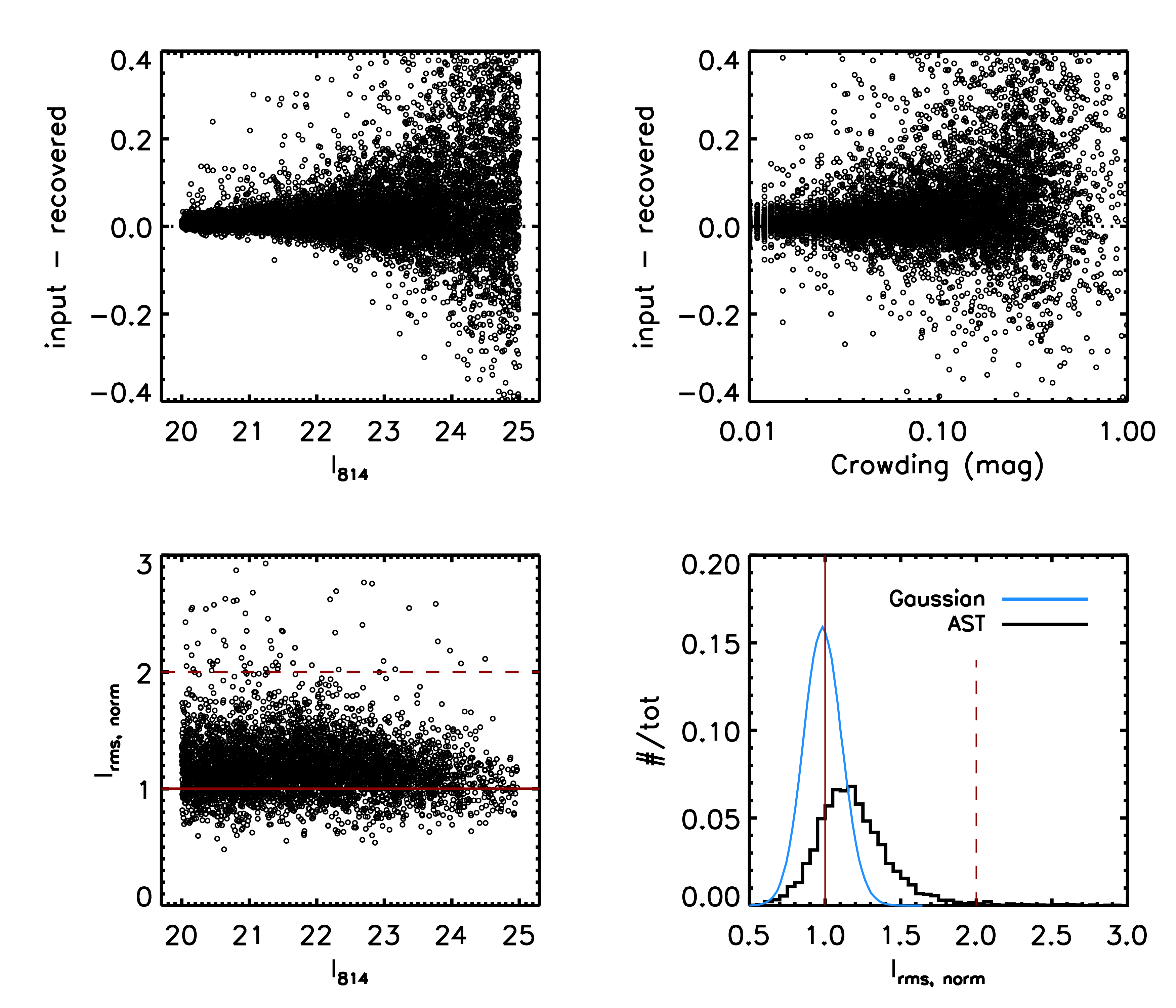
We injected fake stars with a uniform distribution of magnitudes from and sampling a range of local stellar densities. The results are shown in Figure 7. In the upper panels we compare the input and recovered magnitudes and do not identify any significant biases as a function of magnitude but do find a bias as a function of the crowding parameter such that more highly crowded regions result in slightly brighter recovered fluxes compared to the input.
The lower panels quantify the variability of the fake star light curves. Recall that the injected stars do not have any intrinsic variability. We define a quantity, as the rms of the error-normalized light curve, i.e., rms where and are the magnitudes and errors of the th visit in the light curve. This quantity is plotted as a function of input magnitude in the lower left panel and as a histogram in the lower right panel. Here we focus only on stars with crowding. In the right panel we also show the expected distribution if the reported errors captured the entire error budget by drawing mock light curves with the reported errors and measuring the normalized rms values from those mock data. As expected, this distribution is centered on 1.0 and has a width determined by the finite number of samples from the light curve (34).
The lower right panel motivates us to consider a value of as a threshold above which the light curve variation reported by DOLPHOT is likely to be real. In our tests % of artificial stars have . This threshold is also plotted in the lower left panel.
In summary, we have applied magnitude corrections to the Cycle 24 photometry that are a function of detector position and time. In addition, we have added 0.02 mag in quadrature to the DOLPHOT reported errors, to capture a host of possible systematic uncertainties at this low level. With these modifications we expect the vast majority of stars with to display genuine temporal variability. Note that for the brightest stars the error budget is dominated by the 0.02 mag systematic uncertainty, so corresponds to a threshold of .
2.4. Quantifying variability
There is a rich literature describing numerous techniques for quantifying variability in astronomical light curves (e.g., Stetson, 1996; Kim et al., 2014; Jayasinghe et al., 2018). Broadly, these techniques fall into two categories: non-parametric statistics of the light curves, e.g., the rms and higher order moments, and period-finding statistics, e.g., the Lomb-Scargle periodogram (Lomb, 1976; Scargle, 1982; VanderPlas, 2018).
Here we consider both approaches to quantifying variability. In the first, we measure moments of the light curve, focusing primarily on the rms. We also consider an error-normalized version of the rms, as defined in the previous section. These quantities are referred to as and for the values computed from the band light curve. In practice we compute the rms (and the error-normalized rms) after iteratively clipping the data.
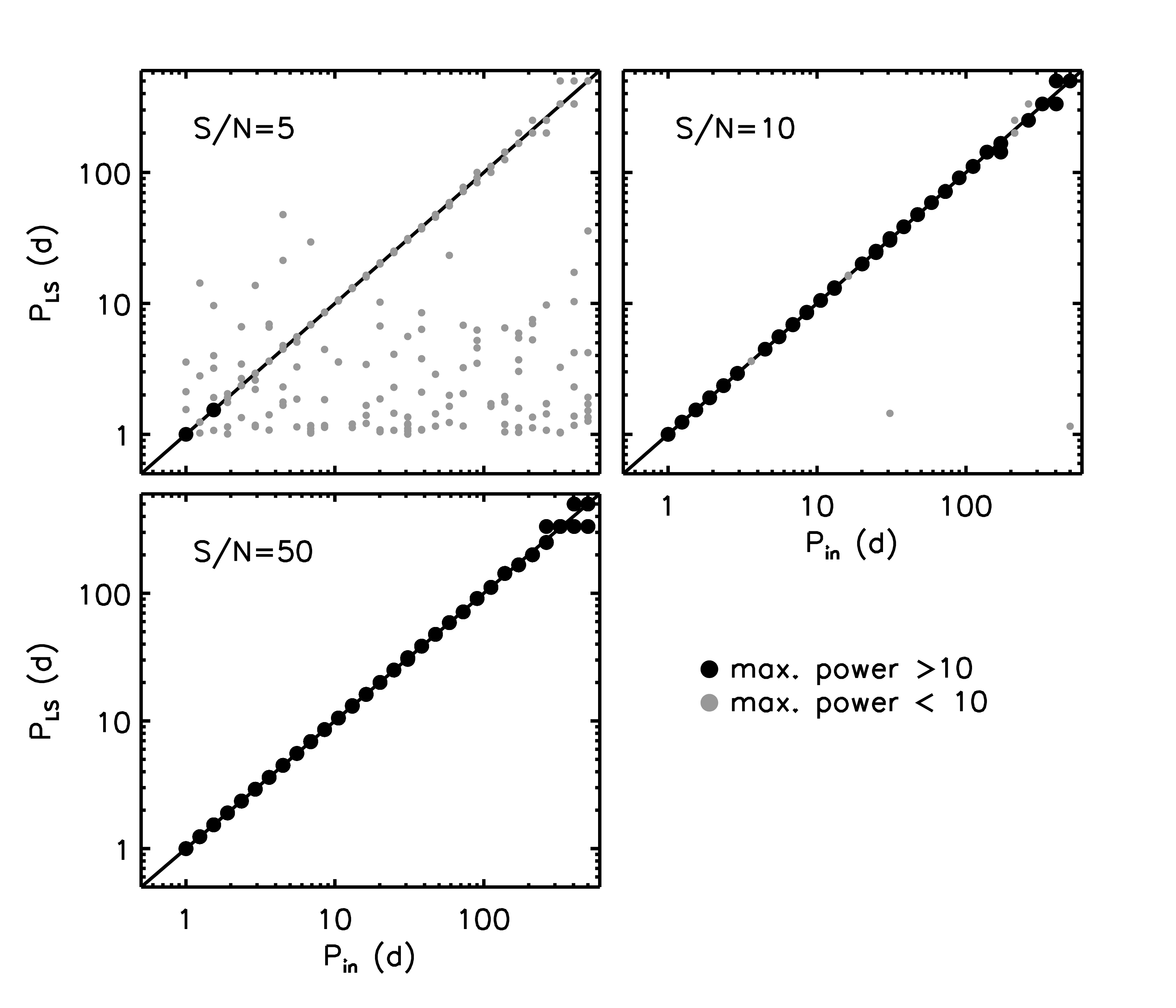
The second approach we consider is applying Lomb-Scargle periodogram analysis to the light curves. For this purpose we use the IDL program scargle.pro. We searched for periods between d using 10,000 frequencies and a false-alarm probability of 0.01. In order to test our ability to recover periods with our cadence and S/N we performed a set of simulations. We created mock light curves with the cadence of our observations at S/N for a range of periods and phases. The light curves are sine waves with unit amplitudes.
The result of this test is shown in Figure 8, where we compare the input and recovered periods for the three S/N values. In each panel there are ten points at each input period representing the ten randomly drawn phases. Points are color-coded by whether their maximum power is or , which is close to a false-alarm probability of 0.01. It is clear that by S/N we are able to recover nearly all input periods to high fidelity. Note that our pseudo-random cadence enables sensitivity to periods at least as short as one day (and likely shorter) for regular, sinusoidal light curves. Furthermore, while we are able to recover periods d even for data that only span one year, we note that this success is due in part to the very simple input light curve shape. In practice, we treat the longer periods ( d) merely as indicative of long timescale variability in the light curve.
We close this section with a few words of caution regarding the Lomb-Scargle analysis. As is well-known, the interpretation of false-alarm probabilities in periodograms is fraught with difficulty (VanderPlas, 2018, and reference therein). The test performed in Figure 8 provides some assurance that a threshold of maximum power , which corresponds approximately to a false-alarm probability of , is adequate for identifying sine-wave variability for data with S/N¿10. In reality the light curves are often not sinusoidal. However, inspection of thousands of light curves has lead us to conclude that this threshold provides a satisfactory balance between minimizing false-positives and identifying light curves with clear variability. Nonetheless we caution that results relying on a light curves selected by maximum power in the periodogram (principally Figure 14) will likely suffer from some degree of contamination and incompleteness.
3. Results
3.1. Variability on day-to-year timescales
In this section we focus on variability measured within our Cycle 24 data, which has sensitivity to variability on day-to-year timescales.
3.1.1 Example light curves
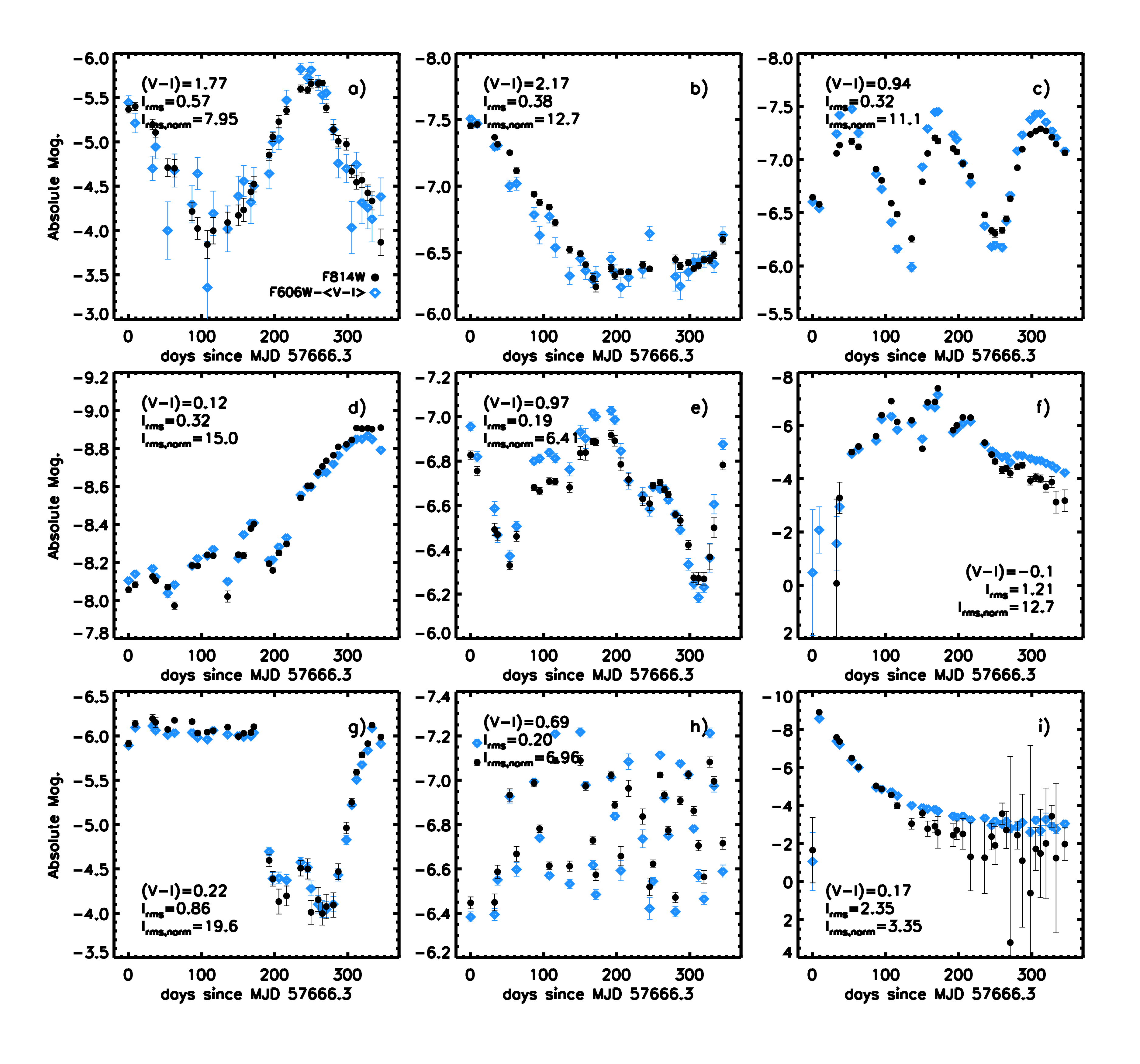
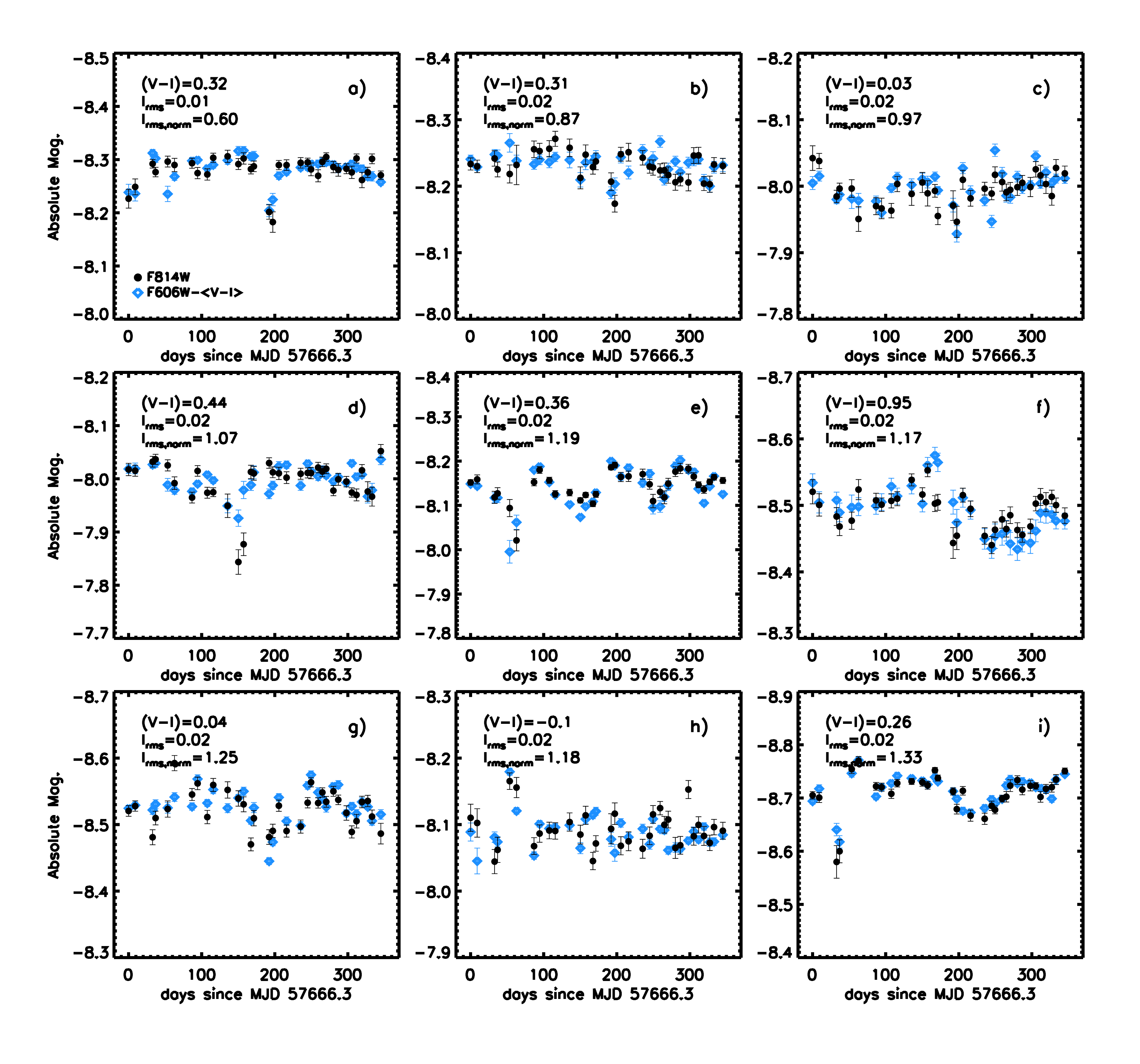
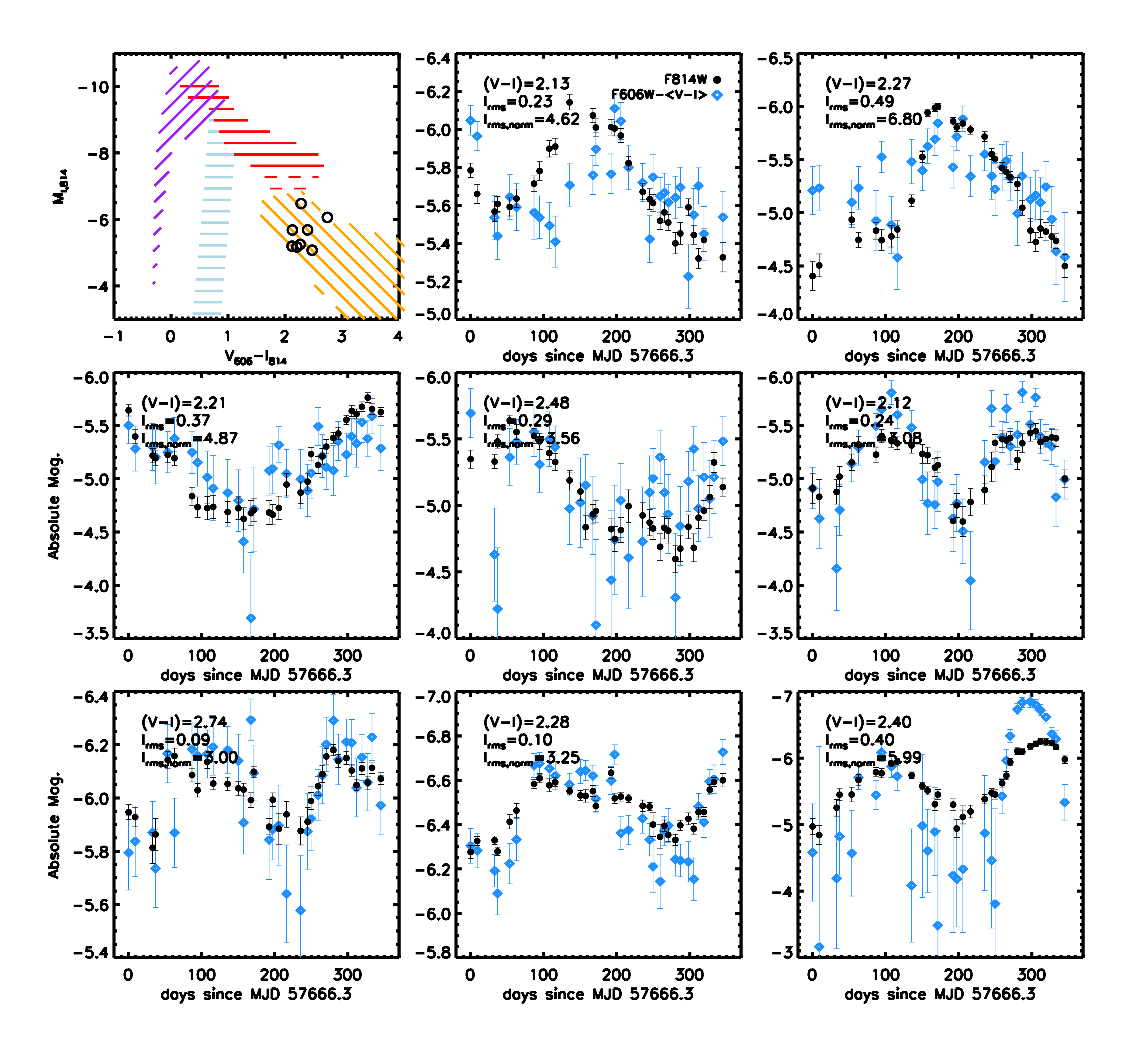
In Figure 9 we highlight unusual and interesting light curves identified in the data. In each panel we show the and band data, with the former shifted by the mean color of the star (recall that the photometry has been corrected for Galactic extinction but not for reddening within M51). We also list the mean color and . One clearly sees a wide range of behavior including periodic light curves, long-term variation, and relatively erratic changes. Specifically, we have selected two fairly typical luminous red giants (a,b), an RV Tau star (c), two luminous blue variables (d-e), an extreme amplitude blue variable (f), an R Coronae Borealis star (g), a bright Cepheid (h), and a very luminous nova (i). R Coronae Borealis (RCB) stars are a class of rare, hydrogen-deficient carbon rich supergiant variables. The RCB star in panel (g), at is perhaps the brightest known star of this class (Tisserand et al., 2009; Tang et al., 2013). Our dataset contains at least five novae and half a dozen very bright RV Tau stars ().
In Figure 9 the color variation is small, and in many cases almost absent, even in the presence of large amplitude variations. For the red stars this suggests that we are witnessing primarily variation in the bolometric luminosity, , of the star, as opposed to variation in . However, for the very blue stars, the bolometric corrections make it difficult to separate changes in from , since changes in the latter result in very small changes in color, see Figure 3. This point highlights the need for simultaneous monitoring of these hot stars in the UV and optical, which would enable measurement of variability in and .
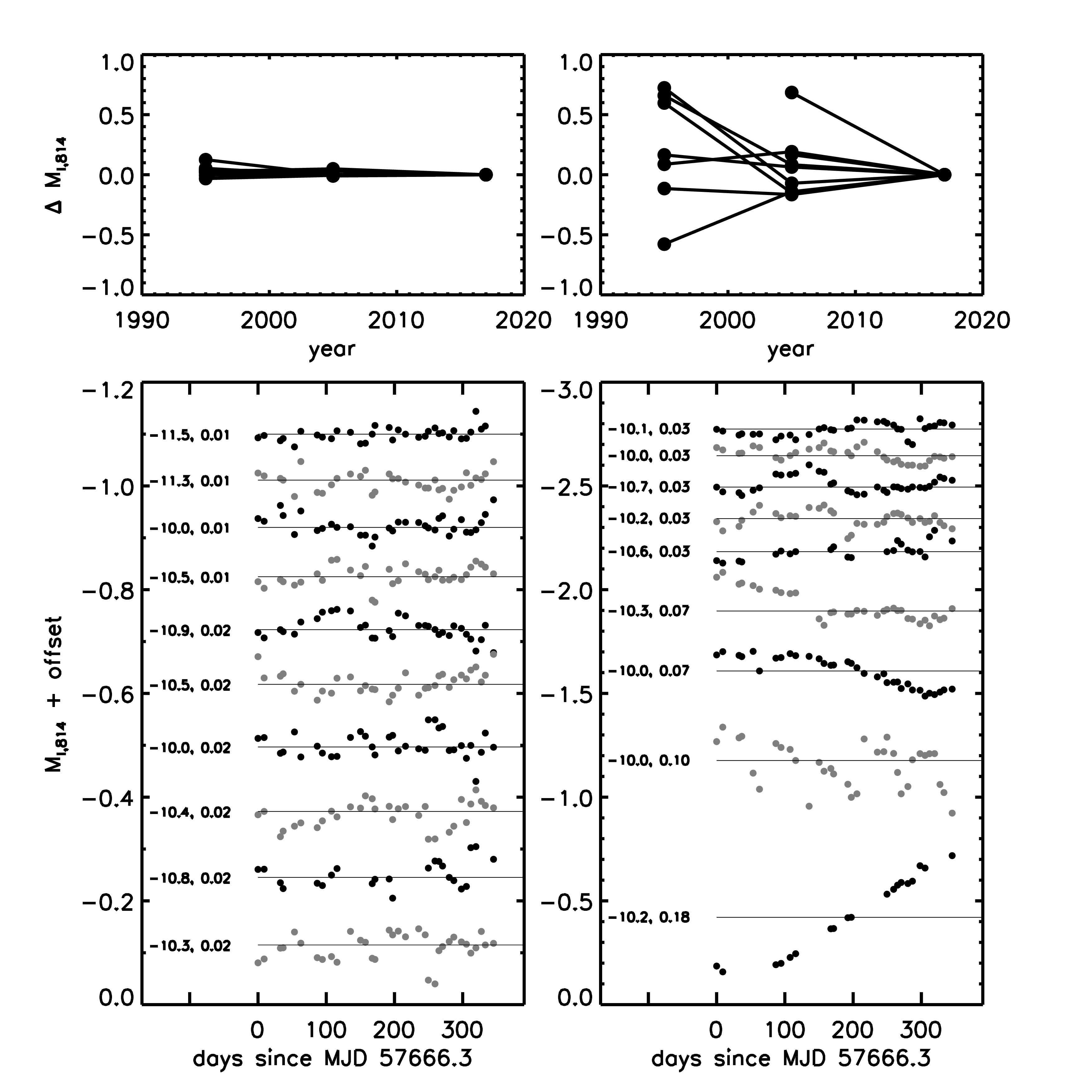
There are 19 stars in our sample that are brighter than . These objects are unlikely to be mis-identified compact star clusters, but they might be unresolved binaries, in which case our luminosities would be over-estimated by at most a factor of two. As discussed in Section 2.2, stars with are all evolved high-mass () stars. We show all 19 light curves in Figure 10. In each panel we plot the band light curves within the Cycle 24 data in the bottom panels and the 22 year baseline light curve including the Cycle 4 and 13 data in the upper panels. In all nine of the light curves in the right panels there is clear variability on month, year, and decade timescales. In contrast, the ten variables on the left show little evidence for variability, on both month-year and decade timescales. From these brightest stars we can already conclude that variability is very common (at least 9/19 or %) amongst the luminous star population.
In Appendix A we present additional light curves of various stellar types, including phase-folded light curves of periodic variables.
3.1.2 The variable star population across luminosity and color
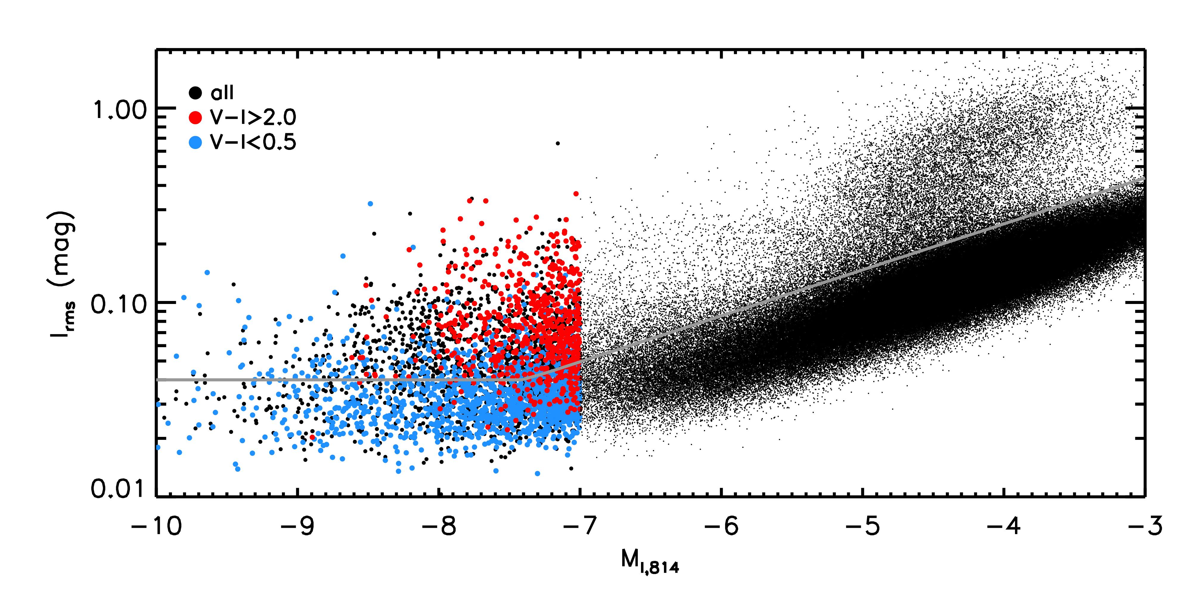
We now turn to a quantitative analysis of the light curve variation for our overall sample. We begin by considering the light curve rms measured in the band, , as a measure of variability. We plot this quantity vs. the absolute band magnitude, , in Figure 11. We also show the variability threshold () as a grey line. The plume of stars at and with large are AGB stars with Mira and SRV-like variability. An important result from this work is that for luminous stars, e.g., , the amplitude of variability is apparently continuous, rather than there being distinct “non-variable” and strongly variable classes. Stars with are shown as larger symbols and are color-coded by their color. Notice that the overwhelming majority of red stars lie above the variability threshold.
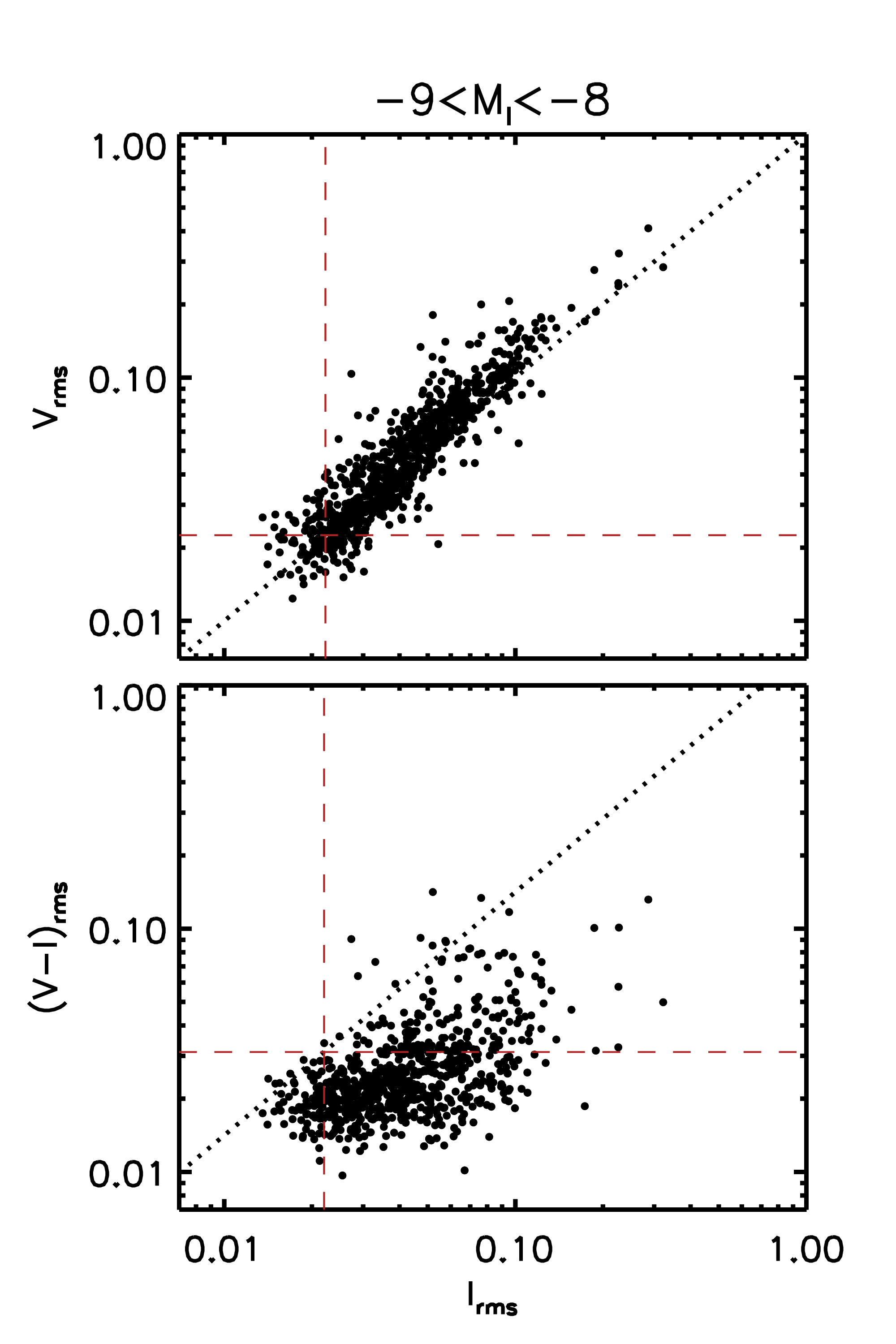
In Figure 12 we compare the , , and light curve rms values for a bright subsample of stars. We chose a narrow range of bright magnitudes for this comparison so that the sample has a small and narrow range of photometric uncertainties, thereby enabling a straightforward interpretation of the computed rms values. We see clearly that and are strongly correlated and there is slightly larger variance in compared to . In contrast, is generally very low and mostly consistent with the photometric uncertainties (the median of the quadrature sum of the and band uncertainties is shown as a horizontal line in the bottom panel). These results imply that the light curves are varying coherently in the and bands. See Appendix A for examples.
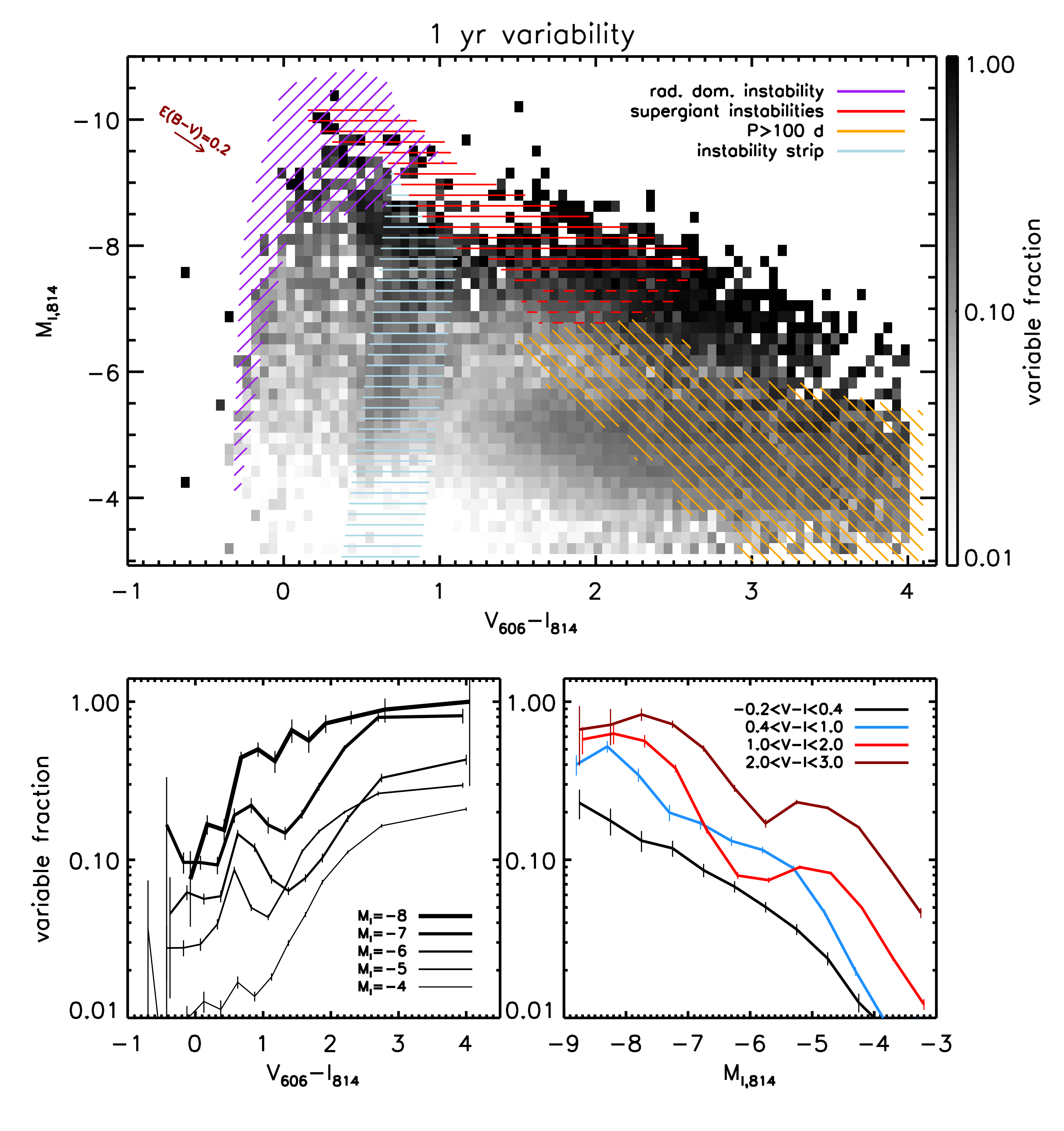
Figure 13 shows the variable star fraction across the CMD. The variable fraction was computed in small color-magnitude bins; at the bright end this fraction is noisy due to Poisson fluctuations. For this reason, in the bottom panels we show the variable star fraction as a function of color in larger bins of luminosity (left panel) and as a function of luminosity in larger bins of color (right panel).
There are many interesting features in this figure. One clearly sees the Cepheid instability strip at , as well as the supergiant variables (e.g., Mira and SRV variables) at red colors. It is interesting that the variability fraction in instability strip is never very high, although it is higher than both bluer and redder colors at fixed magnitude. There appears to be two populations of variables at red colors, which is also apparent in the lower right panel. This is likely due to RSGs at the bright end and AGB stars at the fainter end. One also sees a high fraction of variability amongst the brightest blue stars. At least some of these are likely LBV candidates. We remind the reader that at essentially every bright blue star is an evolved massive star (see Figure 3).
We also show in this figure a reddening vector whose length corresponds to , which we regard as a typical value for internal reddening within a metal-rich spiral galaxy. In a face-on disk galaxy like M51, where most of the dust and gas are confined to the mid-plane, we can expect roughly half of the older stars (in front of the disk) to experience very little attenuation, and roughly half (behind the disk) to experience significant attenuation. For young stars still embedded in their natal clouds we might expect overall higher levels of extinction. It is beyond the scope of this paper to attempt to model these effects; we simply note them here as possible complicating factors when interpreting the observed CMDs. See e.g., Dalcanton et al. (2015) for a sophisticated treatment of dust extinction in a spiral galaxy (M31).
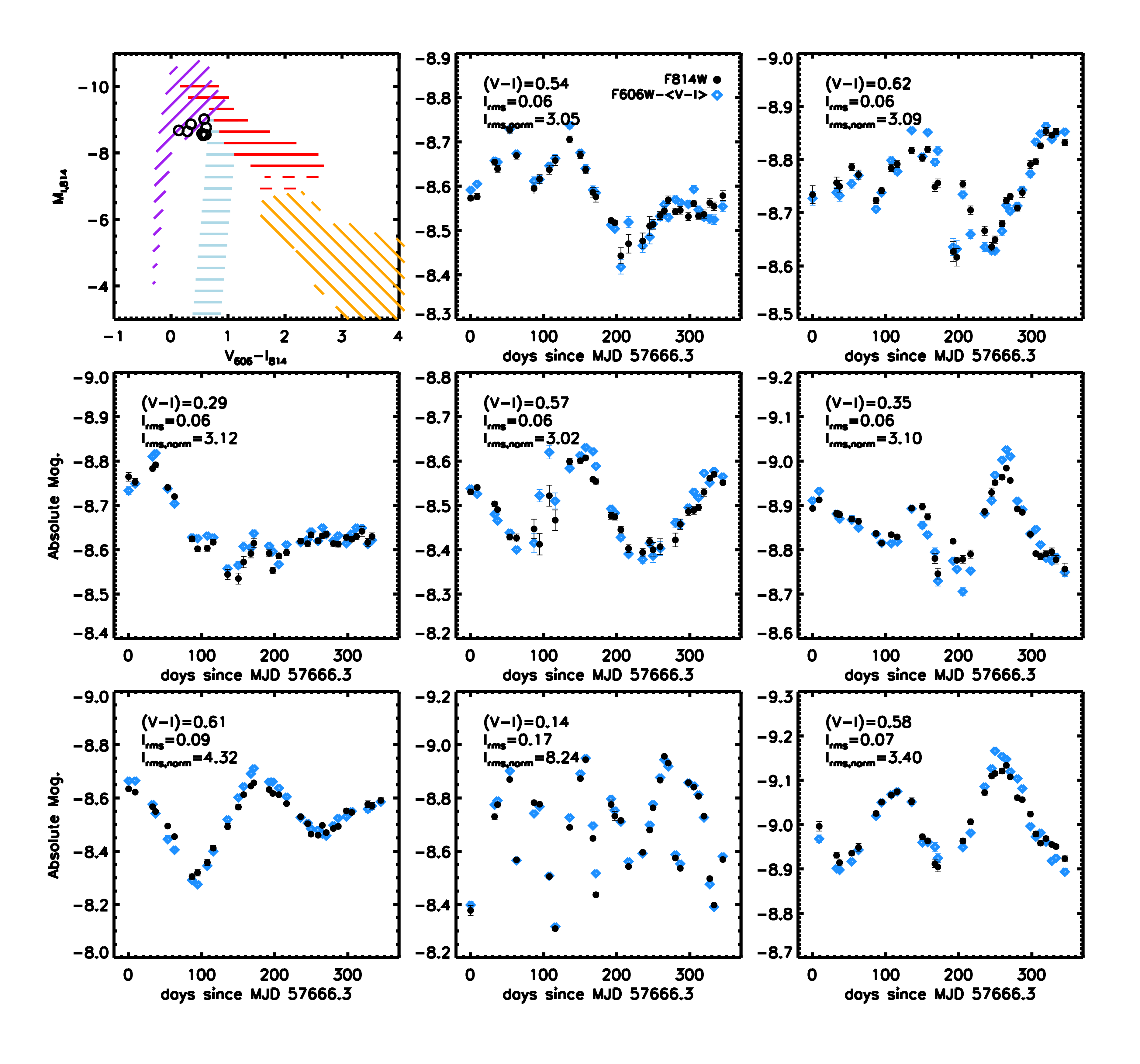
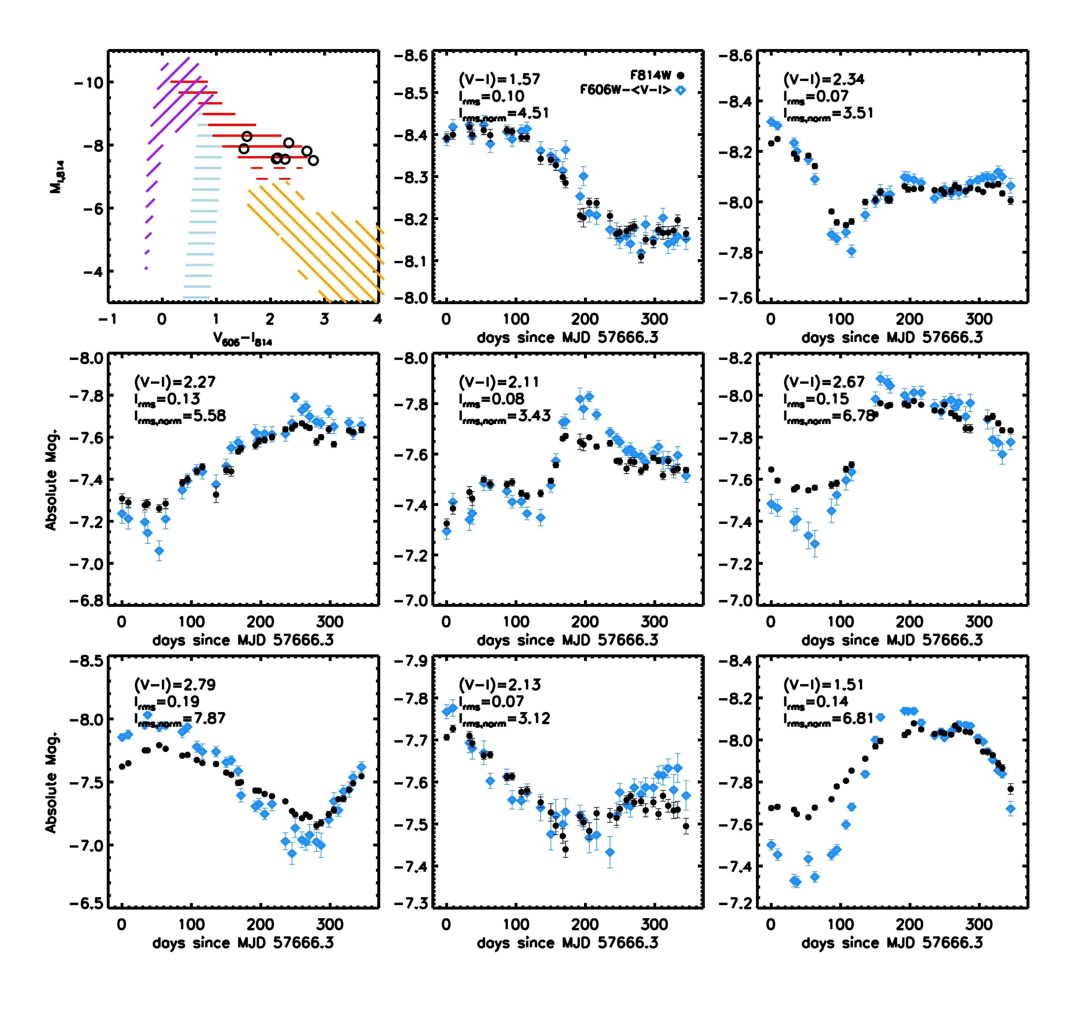
We also show in the upper panel of Figure 13 regions where theoretical models predict variability. The instability strip is estimated from (Paxton et al., 2015) with a width meant to approximate both our data and the LMC Cepheids from OGLE (Soszyński et al., 2015). The supergiant instability region is estimated by applying the pulsation growth rate equation from Yoon & Cantiello (2010) to our MIST stellar tracks and marking the region where the growth rate is . Yoon & Cantiello (2010) find that only stars with pulsate, and they only consider stars up to . Here we mark stars with RSG instabilities in the mass range as solid red lines and as dashed lines. Notice that instabilities at lower masses seem to be required to reproduce the observed region of variability in our data.
We also consider regions where the fundamental pulsation mode of an evolved giant would have a period d; this is indicated by the orange hatched region. For the cool stars we have included the effects of circumstellar dust in the model predictions following Villaume et al. (2015). This has a relatively minor effect on the observed CMD except for the lower-mass AGB stars, which, having intrinsically lower , tend to produce large quantities of dust in their final stages of evolution.
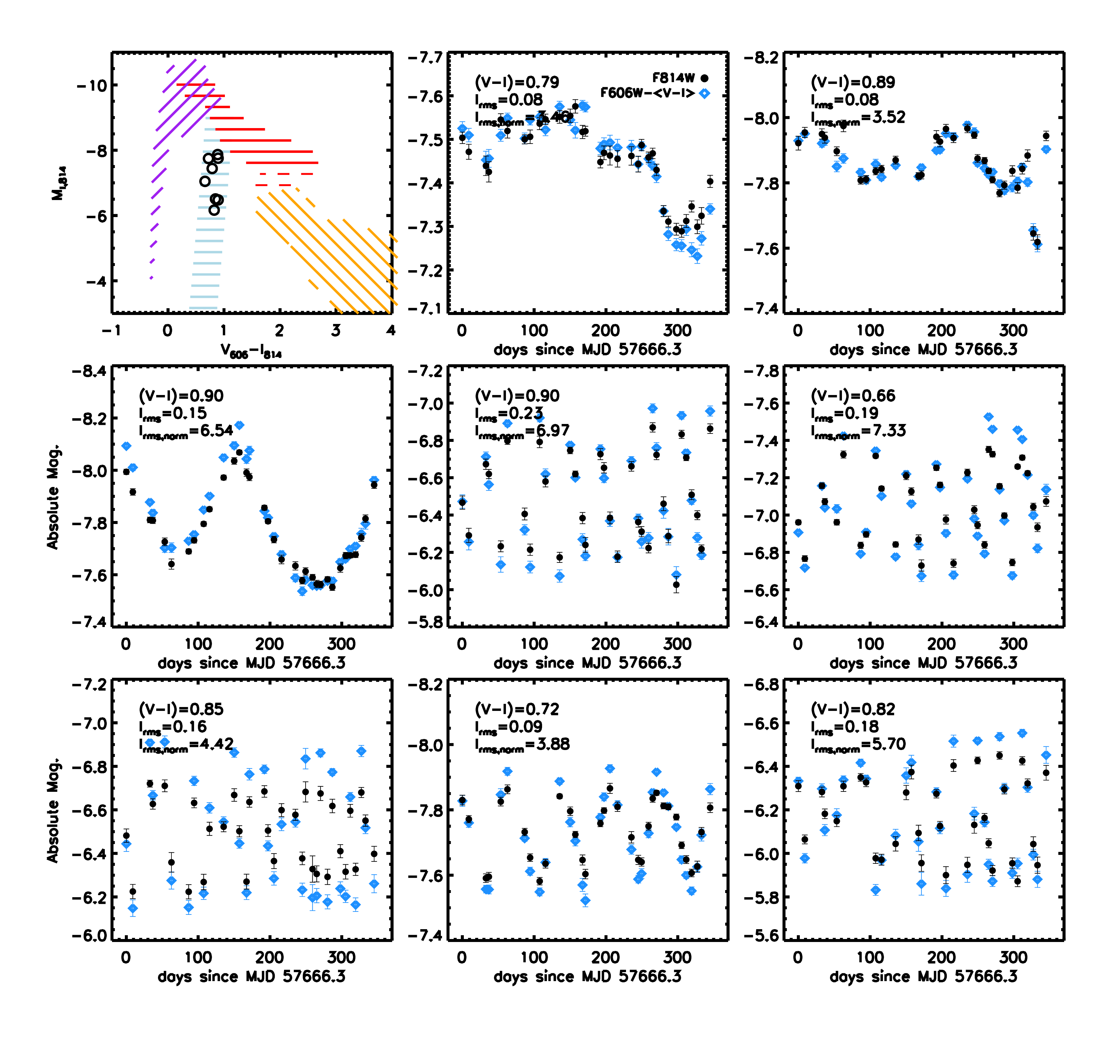
Finally, we consider instabilities that may arise from radiation-dominated envelopes in massive stars (e.g., Paxton et al., 2013; Jiang et al., 2015; Owocki, 2015, and references therein). In evolved massive stars conditions can arise in which a portion of the envelope is some combination of radiation-dominated (), approaching the local Eddington limit, and experiencing a density inversion. The ultimate cause of these conditions is believed to be the iron opacity bumps at K and K. It is difficult or perhaps impossible to properly model this phase of stellar evolution in 1D, but our goal here is simply to use our 1D MIST models to identify periods in the evolution of massive stars when these conditions arise (see Jiang et al., 2015, 2017, for examples of 3D simulations relevant to this phenomenon). Specifically, we identify the region in the CMD where the MIST models satisfy gradt_excess_alpha, where this internal MESA variable is a function of two additional variables, and ; see Paxton et al. (2013) for details. Our particular choice of 0.5 is somewhat arbitrary and the particular value will change the exact boundary of the purple hatched region in Figure 13. Our goal is merely to illustrate where stars in this phase are expected to lie in CMD space.
Overall, the broad agreement between the expected and observed regions of instability is encouraging. However, the correspondance is not perfect. There are blue variables at fainter magnitudes than predicted by our simple prescription for identifying radiation dominated envelopes of massive stars. At cool temperatures, the predicted lower-mass limit of RSG instabilities of by Yoon & Cantiello (2010) is unable to account for the lower luminosity variables in our sample. Extending their instability criterion to results in better agreement with the data. The models are not able to reproduce the colors of the coolest variables. We have adopted a simple prescription for circumstellar dust around these evolved stars; more detailed modeling may be required for these very cool stars. The onset of fundamental mode pulsations with d does a good job of reproducing the location of the lower-luminosity cool variables, although the data include a population of warmer variables at that are not predicted by (solar metallicity) fundamental mode pulsations with d. We leave a more detailed comparison of the observed and theoretical variability regions for future work.
The bottom panels of Figure 13 shows the variability fraction, as a function of luminosity and color. The variability fraction is a strongly increasing function of both luminosity and color with interesting non-monotonic behavior at the color of the Cepheid instability strip (bottom left panel) and at amongst the redder stars (bottom right panel). The variability fraction exceeds 50% for RSGs, which are red and brighter than . This variability fraction is in broad agreement with recent work in M31, where Soraisam et al. (2018) found that all RSGs brighter than show evidence for variability (the typical RSG color is ). Amongst the bluest stars, the variability fraction increases to % for the brightest stars.
We emphasize that the variability fractions quoted here are lower limits. As noted in previous sections, our data are not sensitive to variability at levels below . Moreover, our threshold for variability is , which is the error-normalized rms. At fainter magnitudes where the errors are larger the amplitude must therefore be larger to pass this variability threshold. One sees this selection effect clearly for the Cepheids in Figure 13 — we are able to identify Cepheids as faint as in our data (see below), but they do not show up here due to the variability criterion.
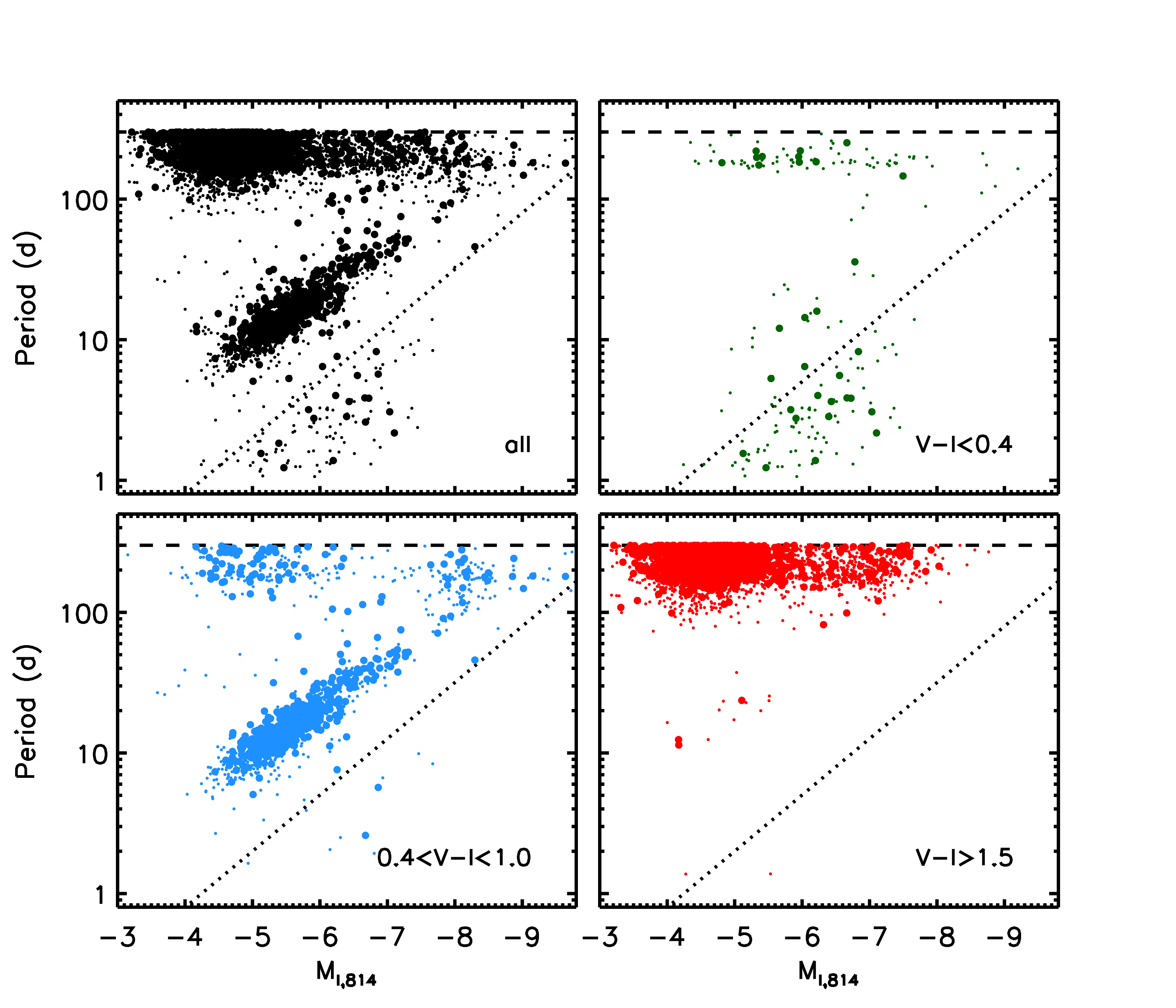
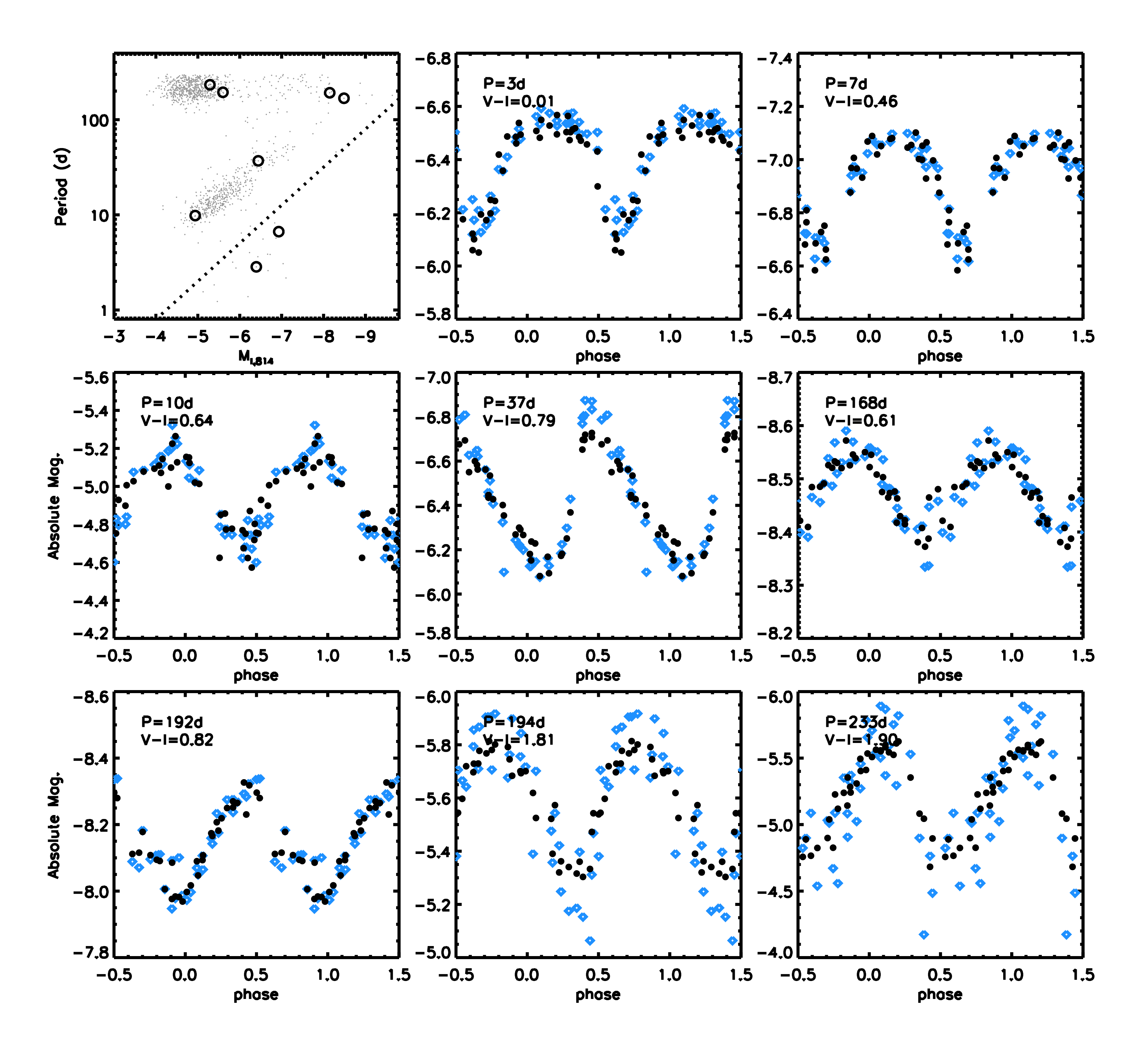
We now consider variables that show periodic behavior as indicated by the Lomb-Scargle periodogram analysis. In Figure 14 we show all variables with and a Lomb-Scargle power with periods of d, separated according to color. Stars with power are shown as large symbols. As discussed in Section 2.4, these selections on the maximum power in the light curve do not necessarily identify a pure nor complete sample, but visual inspection has lead us to conclude that these values identify large fractions of the underlying variables with low levels of contamination. We also emphasize that the stars with periods d should be interpreted with caution — it is difficult if not impossible to reliably measure such long periods with data spanning only one year. However, visual inspection reveals that such stars are clearly variable on long timescales; see Figure 22 for examples. We therefore recommend interpreting stars with d periods as showing clear signs of long timescale variability but with periods that are poorly determined.
Several distinct classes of objects are seen in this figure. The Cepheid Leavitt Law shows up clearly at . The dotted line is meant to guide the eye — based on visual inspection, stars below this line appear to be eclipsing binaries. The red stars are almost exclusively of long periods, except for a few stars at periods of d which upon inspection are highly reddened Cepheids. There is a curious population of long period ( d) very blue stars, although the light curves in these cases are relatively erratic and the derived periods are questionable. Given the relatively short baseline of our Cycle 24 data and the often somewhat irregular (or at least not perfectly sinusoidal) light curves, it is difficult to finely resolve the various classes of long period variables seen in longer baseline data (e.g., Soszyński et al., 2009).
3.2. Variability on decade timescales
The archival HST data obtained in 1995 and 2005 allow us to probe stellar variability on decade timescales amongst 18,000 stars brighter than in both datasets. The 2005 data are both substantially deeper and of higher quality (ACS vs. WFPC2) and so most of the discussion in this section focuses on comparing our Cycle 24 data to the 2005 data.
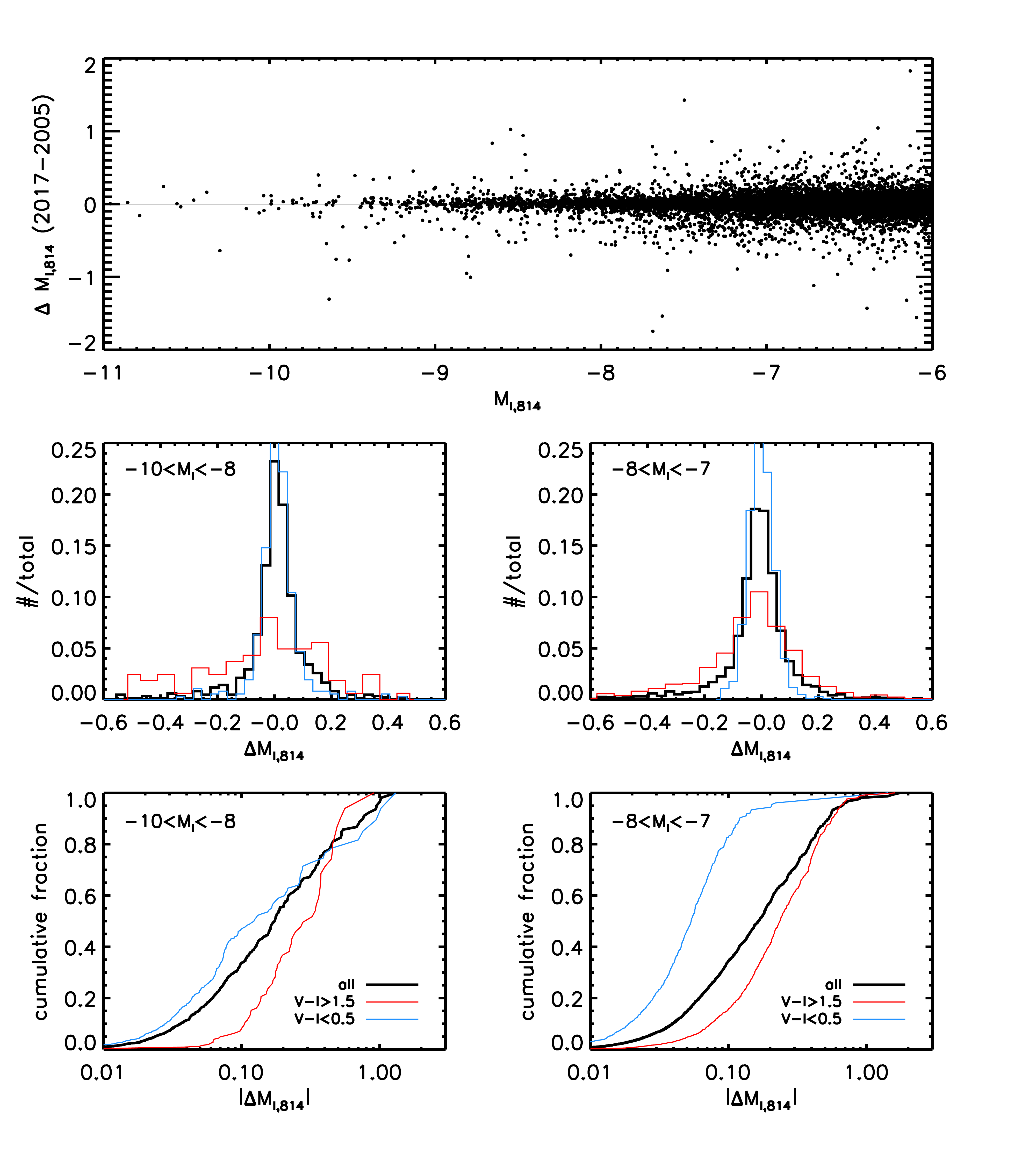
In Figure 15 we plot the change in band magnitude between the Cycle 24 data (referred to as the ‘2017’ data throughout this section) and the 2005 archival data. The upper panel shows as a function of , the middle panels show and the differential distribution of separated by color, and the lower panels show the cumulative distribution of , also split according to the Cycle 24 color. In the lower sets of panels the data are separated into two magnitude bins. The distribution of variability amplitudes in the top panel is consistent with being drawn from a single function of the form . This suggests that the large amplitude variables are simply the tail of a distribution rather than being a special class of objects.
At the distribution shows a weak dependence on color and implies that % of such stars have varied by mag over 12 years and % have varied by mag over the same interval. By there is a much stronger color-dependence such that only % of blue stars varies by more than 0.1 mag, compared to 80% of red stars. Variability exceeding 1 mag is extremely rare, occurring in only 14 stars out of the 18,000 brighter than . Our Cycle 24 data covers 40% of the band flux of M51 and so we can conclude that a typical metal-rich star-forming galaxy contains stars brighter than that vary by more than one mag on decade timescales.
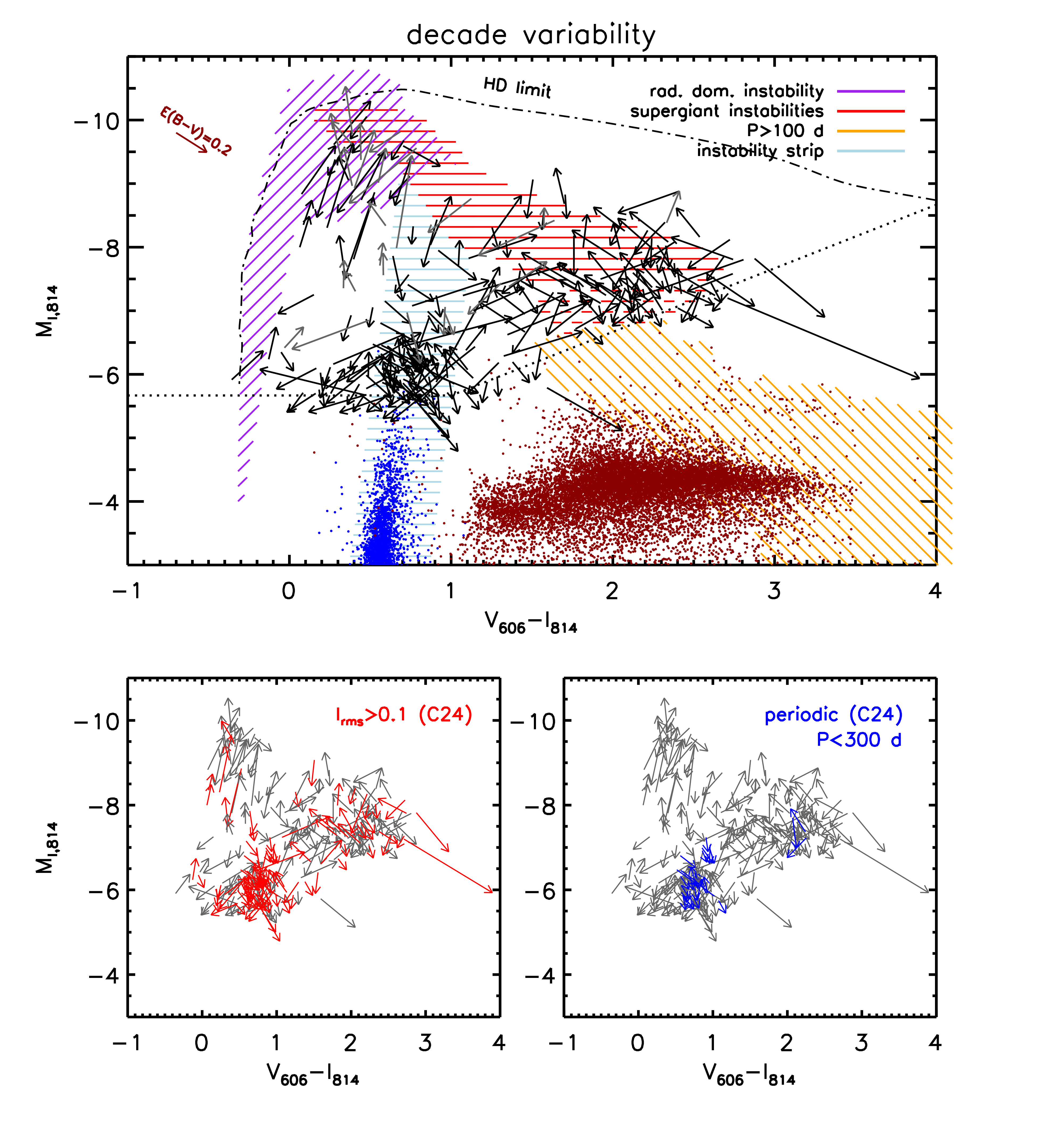
In Figure 16 we show the change in color and magnitude on decade timescales. In this figure it was necessary to include several additional cuts on the data, owing to the varying depths of the Cycle 4 and 13 data. For the Cycle 13 data we require and magnitude errors of in both filters. This yields an approximate color-dependent lower limit indicated by the dotted line in the upper panel. We require similar magnitude precision for the Cycle 4 data, which results in even effective brighter limits owing to the short exposure time of those data. We select variable stars as those with in either the 1995-2005 or 2005-2017 intervals. In the upper panel, black arrows show change from 2005 to 2017 and grey arrows show change from 1995-2005. Notice that in some cases the grey and black arrows are connected, indicating that a single star has varied significantly in both intervals.
In this figure we also indicate regions where stellar variability is expected on theoretical grounds (see also Figure 13), and the Humphreys-Davidson limit (Humphreys & Davidson, 1979), which is an empirical luminosity boundary determined from stars in the Galaxy and Magellanic Clouds. We also show the locations of Mira and SRV variables from the LMC(Soszyński et al., 2009) and LMC Cepheids (Soszyński et al., 2015) for reference. Notice that the sample of LMC variables terminates around , likely owing to the fact that the LMC is a much lower mass galaxy compared to M51 and so lacks these rare, bright stars.
In the lower panels of Figure 16 we highlight those variables that show strong and/or periodic variability within our Cycle 24 data. In the left panel we highlight stars with and in the right panel we highlight stars that show strong evidence for periodic behavior in their band light curves with periods d. RSGs usually have periods well in excess of 300 d (e.g., Soraisam et al., 2018), so it is not surprising that few of the RSGs are labeled as periodic within our Cycle 24 data. Only a fraction of stars with large decade-scale variability also show large amplitude variability on one year timescales. Nonetheless, nearly all of the stars shown as arrows in the lower left panel do harbor statistically-significant evidence for variability within our Cycle 24 data, as defined by our metric . This result, combined with the results of Figure 13, suggests a picture in which nearly all luminous, evolved stars vary on year timescales, albiet with small amplitudes, while on decade timescales these same stars occasionally undergo much larger changes in monochromatic fluxes.
As in Figure 13, it is striking that in Figure 16 the majority of the decade timescale variables lie in regions of the CMD where variability is expected on theoretical grounds.
Finally, we have also searched for stars that have disappeared between 2005 and 2017. There are 20,000 stars brighter than in the 2005 data, which includes all of the RSGs with initial masses . All of these stars are still present in 2017. Kochanek et al. (2008) estimate that it would require monitoring supergiants over a year in order to witness an event of some kind, whether a supernova or a disappearing star (failed supernova). Our baseline of 12 years reduces the number of necessary stars to , so in monitoring “only” 20,000 stars it is not surprising that we have not seen a disappearing star. If we expand the luminosity to include the more luminous AGB stars, , we again find no disappearing stars among the 66,000 stars above this magnitude limit (and with a crowding parameter in the 2005 data ).
4. Summary
In this paper we have presented a complete census of stellar variability amongst the luminous star population in the face-on spiral galaxy M51. Our Cycle 24 data in combination with archival Cycle 4 and 13 data enabled sensitivity to stellar variability on day to decade timescales. We now summarize our main results.
-
•
Stellar variability is ubiquitous. The variability fraction is % for stars with ; this fraction reaches % for the brightest red stars (RSGs). A wide variety of light curve behavior is seen amongst these bright stars, with smooth, long-timescale variability more common for redder stars, and erratic variability common for the blue stars, with amplitudes often exceeding one mag. The color variation is modest for these large amplitude variables, suggesting at least for the redder stars that we are witnessing variation in over time.
-
•
Variable stars occupy well-defined regions in the CMD. These regions correspond to the instability strip, the location of RSGs and AGB stars (Miras and SRVs), and the locations where massive stars are expected to exhibit radiation-dominated and hence unstable outer envelopes. There is broad qualitative agreement between observed and predicted locations of variables in the CMD, but there are several locations that require further study, including the faint RSGs and the luminous blue variables.
-
•
Stars experiencing variability on both short (month-year) and long (decade) timescales is common but not universal. We identify many cases where a star changes in brightness by mag on a decade timescale but is approximately constant () on month-year timescales. This is suggestive of periods of instability followed by periods of quiescence, or perhaps very long timescale variability.
-
•
The amplitude of variability for luminous stars () on both month-year and decade timescales is consistent with a single, continuous distribution from small to large amplitudes. In other words, there is no evidence in our data for distinct classes of large and small amplitude variables amongst the most luminous stars. This suggests for example that LBVs are the extreme end of a continuum of variability amplitudes.
A key missing piece to our analysis of variability in M51 is physical parameters for the stars, especially and . Archival through band data do exist and overlap with the footprint of our Cycle 24 data, but they were taken at different epochs, which makes them less useful for estimating stellar parameters of variable stars. Moreover, for the hottest stars, UV data is essential for accurate stellar parameters. An important next step is to acquire simultaneous UV–NIR photometry in order to measure accurate , , and reddening values on a star-by-star basis.
In the near future we can expect similar censuses to become available in M31 (via PTF data) and in the Galaxy (via Gaia data). Large all-sky monitoring efforts currently planned and underway, including the Zwicky Transient Factory (ZTF) and the Large Survey Synoptic Telescope (LSST), will enable the measurement of stellar variability throughout the Local Group. These studies of variability will offer powerful and novel probes of stellar interiors and short lived phases of stellar evolution, and will require an equally concerted effort from stellar modelers in order to bright to light the basic (and not so basic) physical processes governing stellar variability.
Appendix A Example light curves
In this Appendix we provide additional example light curves associated with several figures in the main text.
Figure 11 showed the vs. . In Figure 17 we show a set of light curves of bright stars from Figure 11. These are randomly drawn from and sorted by . It is clear from these examples that the variability is real . From inspection of all the light curves for the brightest stars, including those not shown in Figure 17, it is also clear that at least some of the stars with are also true variables, so we believe that the quoted variability fraction at the bright end is indeed a lower limit.
In Figures 18–21 we present example light curves of the variable stars from various regions of the CMD shown in Figure 13. In each figure we highlight stars in one of the four hatched regions of instability.
In Figure 22 we show phase-folded light curves of periodic variables drawn from several locations in the period-luminosity plane (see Figure 14). The shortest period variables are likely eclipsing binaries.
Appendix B Photometry and Derived Data Products
In this Appendix we provide an overview of the fits binary file containing the catalog of stars and derived parameters used in this paper. As noted in the main text, the catalog includes all stars with a DOLPHOT object type (star), band crowding , band sharpness, sharp, , a final band S/N and detections in the band for least five epochs. We include all stars with , resulting in 72,623 entries. Table 1 provides a description of the fits file contents.
| column | label | description |
|---|---|---|
| 1 | RA | Right Ascension in decimal degrees (J2000) |
| 2 | DEC | Declination in decimal degrees (J2000) |
| 3 | MAGV0_C24 | magnitude of combined Cycle 24 data |
| 4 | ERRV0_C24 | error of combined Cycle 24 data |
| 5 | CHIV0_C24 | parameter of combined Cycle 24 data |
| 6 | SHARPV0_C24 | sharpness parameter of combined Cycle 24 data |
| 7 | CROWDV0_C24 | crowding parameter of combined Cycle 24 data |
| 8 | MAGI0_C24 | magnitude of combined Cycle 24 data |
| 9 | ERRI0_C24 | error of combined Cycle 24 data |
| 10 | CHII0_C24 | parameter of combined Cycle 24 data |
| 11 | SHARPI0_C24 | sharpness parameter of combined Cycle 24 data |
| 12 | CROWDI0_C24 | crowding parameter of combined Cycle 24 data |
| 13 | MAGV_C24 | Individual epoch magnitudes for Cycle 24 data |
| 14 | ERRV_C24 | Individual epoch errors for Cycle 24 data |
| 15 | MAGI_C24 | Individual epoch magnitudes for Cycle 24 data |
| 16 | ERRI_C24 | Individual epoch errors for Cycle 24 data |
| 17 | MAG_HH | and magnitudes of 2005 data |
| 18 | ERR_HH | and errors of 2005 data |
| 19 | CHI_HH | and parameters of 2005 data |
| 20 | SHARP_HH | and sharpness parameters of 2005 data |
| 21 | CROWD_HH | and crowding parameters of 2005 data |
| 22 | MAG_95 | and magnitudes of 1995 data |
| 23 | ERR_95 | and errors of 1995 data |
| 24 | CHI_95 | and parameters of 1995 data |
| 25 | SHARP_95 | and sharpness parameters of 1995 data |
| 26 | CROWD_95 | and crowding parameters of 1995 data |
| 27 | MATCH_TO_HH_95 | Matched separation between the C24 and Archival catalogs (pixels) |
| 28 | MAG_95_F606W | Converted magnitude for 1995 data |
| 29 | MAG_HH_F606W | Converted magnitude for 2005 data |
| 30 | LS_PERIOD_V | Lomb-Scargle period at maximum power in |
| 31 | LS_MAXPOWER_V | Lomb-Scargle maximum power in |
| 32 | LS_PERIOD_I | Lomb-Scargle period at maximum power in |
| 33 | LS_MAXPOWER_I | Lomb-Scargle maximum power in |
| 34 | RMS_V | rms of light curve () |
| 35 | RMS_I | rms of light curve () |
| 36 | RMSNORM_V | error-normalized rms of light curve () |
| 37 | RMSNORM_I | error-normalized rms of light curve () |
References
- Alcock et al. (1997) Alcock, C., Allsman, R. A., Alves, D., et al. 1997, ApJ, 486, 697
- Bohlin (2016) Bohlin, R. C. 2016, AJ, 152, 60
- Borucki et al. (2010) Borucki, W. J., Koch, D., Basri, G., et al. 2010, Science, 327, 977
- Calzetti et al. (2005) Calzetti, D., Kennicutt, Jr., R. C., Bianchi, L., et al. 2005, ApJ, 633, 871
- Catelan & Smith (2015) Catelan, M. & Smith, H. A. 2015, Pulsating Stars
- Chambers et al. (2016) Chambers, K. C., Magnier, E. A., Metcalfe, N., et al. 2016, ArXiv:1612.05560
- Choi et al. (2016) Choi, J., Dotter, A., Conroy, C., et al. 2016, ApJ, 823, 102
- Conroy et al. (2015) Conroy, C., van Dokkum, P. G., & Choi, J. 2015, Nature, 527, 488
- Dalcanton et al. (2015) Dalcanton, J. J., Fouesneau, M., Hogg, D. W., et al. 2015, ApJ, 814, 3
- Dalcanton et al. (2012) Dalcanton, J. J., Williams, B. F., Lang, D., et al. 2012, ApJS, 200, 18
- Dolphin (2000) Dolphin, A. E. 2000, PASP, 112, 1383
- Drake et al. (2014) Drake, A. J., Graham, M. J., Djorgovski, S. G., et al. 2014, ApJS, 213, 9
- Eyer & Mowlavi (2008) Eyer, L. & Mowlavi, N. 2008, in Journal of Physics Conference Series, Vol. 118, Journal of Physics Conference Series, 012010
- Freedman et al. (1994) Freedman, W. L., Hughes, S. M., Madore, B. F., et al. 1994, ApJ, 427, 628
- Hartman et al. (2004) Hartman, J. D., Bakos, G., Stanek, K. Z., & Noyes, R. W. 2004, AJ, 128, 1761
- Hartman et al. (2006) Hartman, J. D., Bersier, D., Stanek, K. Z., et al. 2006, MNRAS, 371, 1405
- Heger et al. (1997) Heger, A., Jeannin, L., Langer, N., & Baraffe, I. 1997, A&A, 327, 224
- Hubble & Sandage (1953) Hubble, E. & Sandage, A. 1953, ApJ, 118, 353
- Humphreys & Davidson (1979) Humphreys, R. M. & Davidson, K. 1979, ApJ, 232, 409
- Humphreys et al. (2017) Humphreys, R. M., Davidson, K., Hahn, D., Martin, J. C., & Weis, K. 2017, ApJ, 844, 40
- Jayasinghe et al. (2018) Jayasinghe, T., Kochanek, C. S., Stanek, K. Z., et al. 2018, ArXiv:1803.01001
- Jiang et al. (2015) Jiang, Y.-F., Cantiello, M., Bildsten, L., Quataert, E., & Blaes, O. 2015, ApJ, 813, 74
- Jiang et al. (2017) —. 2017, ApJ, 843, 68
- Johnson et al. (2012) Johnson, L. C., Seth, A. C., Dalcanton, J. J., et al. 2012, ApJ, 752, 95
- Justham et al. (2014) Justham, S., Podsiadlowski, P., & Vink, J. S. 2014, ApJ, 796, 121
- Kasliwal et al. (2011) Kasliwal, M. M., Cenko, S. B., Kulkarni, S. R., Ofek, E. O., Quimby, R., & Rau, A. 2011, ApJ, 735, 94
- Kim et al. (2014) Kim, D.-W., Protopapas, P., Bailer-Jones, C. A. L., Byun, Y.-I., Chang, S.-W., Marquette, J.-B., & Shin, M.-S. 2014, A&A, 566, A43
- Kochanek et al. (2008) Kochanek, C. S., Beacom, J. F., Kistler, M. D., et al. 2008, ApJ, 684, 1336
- Kourniotis et al. (2014) Kourniotis, M., Bonanos, A. Z., Soszyński, I., et al. 2014, A&A, 562, A125
- Krist (1995) Krist, J. 1995, in Astronomical Society of the Pacific Conference Series, Vol. 77, Astronomical Data Analysis Software and Systems IV, ed. R. A. Shaw, H. E. Payne, & J. J. E. Hayes, 349
- Law et al. (2009) Law, N. M., Kulkarni, S. R., Dekany, R. G., et al. 2009, PASP, 121, 1395
- Leavitt (1908) Leavitt, H. S. 1908, Annals of Harvard College Observatory, 60, 87
- Lomb (1976) Lomb, N. R. 1976, Ap&SS, 39, 447
- Martin & Humphreys (2017) Martin, J. C. & Humphreys, R. M. 2017, AJ, 154, 81
- Massey et al. (2007) Massey, P., McNeill, R. T., Olsen, K. A. G., Hodge, P. W., Blaha, C., Jacoby, G. H., Smith, R. C., & Strong, S. B. 2007, AJ, 134, 2474
- Massey et al. (2009) Massey, P., Silva, D. R., Levesque, E. M., Plez, B., Olsen, K. A. G., Clayton, G. C., Meynet, G., & Maeder, A. 2009, ApJ, 703, 420
- McQuinn et al. (2016) McQuinn, K. B. W., Skillman, E. D., Dolphin, A. E., Berg, D., & Kennicutt, R. 2016, ApJ, 826, 21
- Mentuch Cooper et al. (2012) Mentuch Cooper, E., Wilson, C. D., Foyle, K., et al. 2012, ApJ, 755, 165
- Nascimbeni et al. (2014) Nascimbeni, V., Bedin, L. R., Heggie, D. C., et al. 2014, MNRAS, 442, 2381
- Owocki (2015) Owocki, S. P. 2015, in Astrophysics and Space Science Library, Vol. 412, Very Massive Stars in the Local Universe, ed. J. S. Vink, 113
- Paxton et al. (2013) Paxton, B., Cantiello, M., Arras, P., et al. 2013, ApJS, 208, 4
- Paxton et al. (2015) Paxton, B., Marchant, P., Schwab, J., et al. 2015, ApJS, 220, 15
- Pojmanski (2002) Pojmanski, G. 2002, Act. Astron., 52, 397
- Rejkuba et al. (2003) Rejkuba, M., Minniti, D., Silva, D. R., & Bedding, T. R. 2003, A&A, 411, 351
- Scargle (1982) Scargle, J. D. 1982, ApJ, 263, 835
- Schlafly & Finkbeiner (2011) Schlafly, E. F. & Finkbeiner, D. P. 2011, ApJ, 737, 103
- Smith (2014) Smith, N. 2014, ARA&A, 52, 487
- Smith & Arnett (2014) Smith, N. & Arnett, W. D. 2014, ApJ, 785, 82
- Smith & Owocki (2006) Smith, N. & Owocki, S. P. 2006, ApJ, 645, L45
- Soraisam et al. (2018) Soraisam, M. D., Bildsten, L., Drout, M. R., et al. 2018, ArXiv e-prints
- Soszyński et al. (2009) Soszyński, I., Udalski, A., Szymański, M. K., et al. 2009, Act. Astron., 59, 239
- Soszyński et al. (2015) —. 2015, Act. Astron., 65, 297
- Stetson (1996) Stetson, P. B. 1996, PASP, 108, 851
- Tammann & Sandage (1968) Tammann, G. A. & Sandage, A. 1968, ApJ, 151, 825
- Tang et al. (2013) Tang, S., Cao, Y., Bildsten, L., et al. 2013, ApJ, 767, L23
- Tisserand et al. (2009) Tisserand, P., Wood, P. R., Marquette, J. B., et al. 2009, A&A, 501, 985
- Udalski (2003) Udalski, A. 2003, Act. Astron., 53, 291
- van Dokkum (2001) van Dokkum, P. G. 2001, PASP, 113, 1420
- VanderPlas (2018) VanderPlas, J. T. 2018, ApJS, 236, 16
- Villaume et al. (2015) Villaume, A., Conroy, C., & Johnson, B. D. 2015, ApJ, 806, 82
- Williams et al. (2014) Williams, B. F., Lang, D., Dalcanton, J. J., et al. 2014, ApJS, 215, 9
- Wood (1979) Wood, P. R. 1979, ApJ, 227, 220
- Yadav & Glatzel (2017) Yadav, A. P. & Glatzel, W. 2017, MNRAS, 471, 3245
- Yoon & Cantiello (2010) Yoon, S.-C. & Cantiello, M. 2010, ApJ, 717, L62