Absolute Distances to Nearby Type Ia Supernovae via Light Curve Fitting Methods

Abstract

We present a comparative study of absolute distances to a sample of very nearby, bright Type Ia supernovae (SNe) derived from high cadence, high signal-to-noise, multi-band photometric data. Our sample consists of four SNe: 2012cg, 2012ht, 2013dy and 2014J. We present new homogeneous, high-cadence photometric data in Johnson-Cousins $BVRI$ and Sloan $g^{\prime}r^{\prime}i^{\prime}z^{\prime}$ bands taken from two sites (Piszkesteto and Baja, Hungary), and the light curves are analyzed with publicly available light curve fitters (MLCS2k2, SNooPy2 and SALT2.4). When comparing the best-fit parameters provided by the different codes, it is found that the distance moduli of moderately-reddened SNe Ia agree within $\lesssim 0.2$ mag, and the agreement is even better ($\lesssim 0.1$ mag) for the highest signal-to-noise $BVRI$ data. For the highly-reddened SN 2014J the dispersion of the inferred distance moduli is slightly higher. These SN-based distances are in good agreement with the Cepheid distances to their host galaxies. We conclude that the current state-of-the-art light curve fitters for Type Ia SNe can provide consistent absolute distance moduli having less than $\sim 0.1$ – 0.2 mag uncertainty for nearby SNe. Still, there is room for future improvements to reach the desired $\sim 0.05$ mag accuracy in the absolute distance modulus.

1 Introduction

Getting reliable absolute distances is of immense importance in observational astrophysics. Supernovae (SNe) in particular play a central role in establishing the extragalactic distance ladder. Distances to Type Ia SNe are essential data for studying the expansion of the Universe (Riess et al., 1998; Perlmutter et al., 1999; Astier et al., 2006; Riess et al., 2007; Wood-Vasey et al., 2007; Kessler et al., 2009; Guy et al., 2010; Conley et al., 2011; Betoule et al., 2014; Rest et al., 2014; Scolnic et al., 2014). SNe Ia are also especially important objects for measuring the Hubble-parameter $H_{0}$ (Riess et al., 2011, 2016; Dhawan et al., 2017), and they play a key role in testing current cosmological models (Benitez-Herrera et al., 2013; Betoule et al., 2014). Their importance has even been strengthened since the release of the cosmological parameters from the Planck mission (Planck Collaboration et al., 2014, 2015), which turned out to be slightly in tension with the current implementation of the SN Ia distance measurements (see Riess et al., 2016, and references therein).

It must be emphasized that the majority of cosmological studies use relative distances to moderate- and high-redshift SNe Ia to derive the cosmological parameters ($\Omega_{m}$, $\Omega_{\Lambda}$, $w$, etc). From this point of view there is no need for having absolute distances, because the relative distances between different SNe/galaxies can be obtained with much better accuracy, especially if the galaxy is in the Hubble-flow ($z\gtrsim 0.1$).

On the other hand, having accurate absolute distances to the nearby galaxies that are not part of the Hubble-flow is very important an astrophysical point of view. Getting reliable estimates for the physical parameters of such galaxies and the objects within them is possible only if we have reliable absolute distances on extragalactic scales.

Thus, investigating the nearest SNe Ia (within $z\lesssim 0.01$) can provide valuable information for various reasons. For example, distances to their host galaxies can be relatively easily determined by several methods, thus, the SN-based distances can be compared directly to those derived independently by using other types of objects and/or methods. Such very nearby galaxies might also serve as “anchors” in the cosmic distance ladder (e.g. NGC 4258, see Riess et al., 2011, 2016), which play an essential role in measuring $H_{0}$.

Table 1: Basic data for the studied SNe

SN	Discovery date	T($B_{max}$)	$\Delta m_{15}(B)$	Host	$z_{host}$	$D_{host}$	$E(B-V)_{MW}$	$\log M_{*}$	References
		(MJD)	(mag)			(Mpc)	(mag)	($M_{\odot}$)
SN 2012cg (catalog )	2012-05-17	56080.0	0.98	NGC 4424	0.001458	16.4	0.018	9.4	1,9,10
SN 2012ht (catalog )	2012-12-18	56295.6	1.27	NGC 3447	0.003559	24.1	0.026	9.3	2,3,9,11
SN 2013dy (catalog )	2013-07-10	56501.1	0.96	NGC 7250	0.003889	20.0	0.135	9.2	4,5,9,12
SN 2014J (catalog )	2014-01-21	56689.7	1.03	M82	0.000677	3.9	0.140	10.5	6,7,8,13

The popularity of SNe Ia as extragalactic distance estimators is mostly due to the fact that their absolute distances can be derived via fitting light curves (LCs) of “normal” Ia events. The LCs of such events obey the empirical Phillips-relation, i.e. intrinsically brighter SNe have more slowly declining LCs in the optical bands (Pskovskii, 1977; Phillips, 1993). Even though nowadays SNe Ia seem to be even better standard candles in the near-infrared (NIR) regime than in the optical (Friedman et al., 2015; Shariff et al., 2016; Weyant et al., 2017), obtaining rest-frame NIR LCs for SNe Ia, except for the nearest and brightest ones, can be challenging. Thus, photometric data taken in rest-frame optical bands can still provide valuable information regarding distance measurements on the extragalactic scale.

One of the main motivations of the present paper is to get absolute distances to some of the nearest and brightest recent SNe Ia by fitting homogeneous, high-cadence, high S/N photometric data with public, widely-used LC-fitting codes. We selected four nearby Type Ia SNe for this project: 2012cg, 2012ht, 2013dy and 2014J. All of them occured in the local Universe, and they were discovered relatively early (more than 1 week before B-band maximum). We have obtained new, densely sampled photometric measurements for each of them in various optical bands, which resulted in light curves extending from pre-maximum epochs up to the end of the photospheric phase. These objects, along with SN 2011fe, belong to the 10 brightest SNe Ia in last decade that were accessible from the northern hemisphere. However, unlike SN 2011fe, all of them were significantly reddened by dust either in the Milky Way or in their hosts, which enabled us to test the performance of the LC-fitters in case of reddened SNe. In addition, their very low redshift ($z<0.01$) eliminated the necessity for K-correction, which could be another possible cause for systematic errors when comparing photometry of SNe having significantly different redshifts (Saunders et al., 2015). It is also important to note that three out of four SNe in our sample have Cepheid-based distances obtained by HST/WFC3, and they were recently used in calibrating $H_{0}$ with an unprecedented 2.4 percent accuracy (Riess et al., 2016).

The basic parameters for the program SNe are collected in Table 1.

In the following we briefly describe the observations (Section 2) and the LC-fitting codes applied (Section 3). Section 4 presents the results from the LC fitting, which are discussed further in Section 5. Section 6 summarizes the main results and conclusions.

2 Observations

Photometry of the target SNe have been carried out at two sites, located $\sim 200$ km apart: at the Piszkéstető station of Konkoly Observatory, Hungary, and at Baja Observatory of the University of Szeged, Hungary. At Konkoly the data were taken with the 0.6m Schmidt telescope through Bessell $BVRI$ filters. At Baja the observations were carried out with the 0.5m BART telescope equipped with Sloan $g^{\prime}r^{\prime}i^{\prime}z^{\prime}$ filters. See Vinkó et al. (2012) for more details on these two instruments.

All data have been reduced using standard IRAF routines. Transformation to the standard photometric systems (Johnson-Cousins/Vega and Sloan/AB for the $BVRI$ and $g^{\prime}r^{\prime}i^{\prime}z^{\prime}$ data, respectively) was computed using catalogued Sloan-photometry for local tertiary standard stars. In the fields of SN 2012cg and SN 2012ht the $BVRI$ magnitudes for the local standards were calculated from their catalogued $g^{\prime}r^{\prime}i^{\prime}z^{\prime}$ magnitudes using the calibration given by Jordi et al. (2006). For SN 2013dy and 2014J the estimated $BVRI$ magnitudes obtained this way were cross-checked by observing Landolt standard fields on a photometric night and re-calibrating the local standards using the zero-points from the Landolt standards. Finally, all $BVRI$ photometry were cross-compared to the Pan-STARRS (PS1) magnitudes of the local standards stars, and small ($\lesssim 0.1$ mag) shifts were applied when needed to bring all the photometry to the same zero-point. The final $BVRI$ magnitudes for the local comparison stars are shown in the Appendix (Table 11, 13, 15 and 18).

Photometry of the SNe was obtained via PSF-fitting using DAOPHOT. The resulting instrumental magnitudes were transformed to the standard systems by applying linear color terms, and the zero points of the transformation are tied to the magnitudes of the local comparison stars.

The final LCs were compared with other published, independent photometry for each SNe, except for SN 2012ht, where no other available photometry was found. We used the data given by Marion et al. (2015b), Pan et al. (2015) and Marion et al. (2015a) for SN 2012cg, 2013dy and 2014J, respectively. A $\sim 0.1$ mag systematic difference was identified between the $B$-band LCs of the heavily-reddened SN 2014J, which was corrected by shifting our data to match those published by Marion et al. (2015a). No such systematic offsets between our data and those from others were found for the remaining three SNe. The final photometric data can be found in the Appendix, in Tables 12, 14, 16, 17 and 19.

3 Analysis

We applied three SN Ia LC-fitters for this study: MLCS2k2 (Riess et al., 1998; Jha et al., 1999; Jha, Riess & Kirshner, 2007), SALT2 version 2.4 (Guy et al., 2007, 2010; Betoule et al., 2014) and SNooPy2 (Burns et al., 2011, 2014). All these, in principle, rely on the Phillips-relation but each code uses different parametrization for fitting the light curve shape and each has different sets of calibrating SNe (“training sets”). There are also other implementations, like SiFTO (Conley et al., 2008) or BayeSN (Mandel et al., 2011), but the first three listed above have been used most frequently in the literature.

Conley et al. (2008) categorized such codes as either “pure LC-fitters” or “distance calculators”. Distance calculators can provide the true absolute distance as a fitting parameter, but they require a training set of SNe having independently obtained absolute distances. Since building such a training set is non-trivial, the calibration of such codes is usually based on a relatively small number of objects. On the contrary, LC-fitters can predict only relative distances, but they can be calibrated using a much larger sample of objects having much more accurate relative distances. Regarding the three codes applied in our study, MLCS2k2 and SNooPy2 are distance calculators, while SALT2 is an LC-fitter, even though it is possible to derive absolute distances from the SALT2 fitting parameters, if needed.

MLCS2k2 (Jha, Riess & Kirshner, 2007) uses the following SN Ia LC model:

$$m_{x}(\varphi)~{}=~{}M_{x}^{0}+\mu_{0}+\eta_{x}A_{V}^{0}+P_{x}\Delta+Q_{x}\Delta^{2},$$ (1)

where $\varphi=t-T_{max}$ is the SN phase in days, $T_{max}$ is the moment of maximum light in the $B$-band, $m_{x}$ is the observed magnitude in the $x$-band ($x=B,V,R,I$), $M_{x}^{0}(\varphi)$ is the fiducial SN Ia absolute LC in the same band, $\mu_{0}$ is the true (reddening-free) SN distance modulus, $\eta_{x}=\zeta_{x}(\alpha_{x}+\beta_{x}/R_{V})$ gives the time-dependent interstellar reddening, $R_{V}$ and $A_{V}^{0}$ are the ratio of total-to-selective absorption and $V$-band extinction at maximum light, respectively, $\Delta$ is the main LC parameter, and $P_{x}(\varphi)$ and $Q_{x}(\varphi)$ are tabulated functions of the SN phase (“LC-vectors”). The absolute magnitudes of SNe in MLCS2k2 have been calibrated using relative distances of more than 150 SNe in the Hubble-flow assuming $H_{0}=65$ km s^-1 Mpc^-1, but later they were tied to Cepheid distances of a smaller sample of SNe Ia host galaxies (Riess et al., 2005).

Contrary to MLCS2k2, SALT2 models the whole spectral energy distribution (SED) of a SN Ia as

$$F_{\lambda}(\varphi)~{}=~{}x_{0}\cdot[M_{0}(\varphi,\lambda)+x_{1}M_{1}(\varphi,\lambda)]\exp[C\cdot C_{L}(\lambda)],$$ (2)

where $F_{\lambda}(\varphi)$ is the phase-dependent rest-frame flux density, $M_{0}(\varphi,\lambda)$, $M_{1}(\varphi,\lambda)$ and $C_{L}(\lambda)$ are the SALT2 trained vectors. The free parameters $x_{0}$, $x_{1}$ and $C$ are the normalization- , stretch- and color parameters, respectively.

Being an LC-fitter, SALT2 does not contain the distance as a fitting parameter. Instead, the distance modulus can be calculated from the following equation (Conley et al., 2011; Betoule et al., 2014; Scolnic & Kessler, 2016):

$$\mu_{0}~{}=~{}m^{*}_{B}-M_{B}+\alpha x_{1}-\beta C.$$ (3)

For the nuisance parameters $\alpha$, $\beta$ and $M_{B}$ we adopted the calibration by Betoule et al. (2014): $M_{B}=-19.17\pm 0.038$, $\alpha=0.141\pm 0.006$, $\beta=3.099\pm 0.075$, and derived the distance moduli from the fitting parameters via Monte-Carlo simulations.

One of the great advantages of SALT2 is that it can be relatively easily applied to data taken in practically any photometric system provided the filter transmission functions are loaded into the code. Because of this and many other reasons, SALT2 became very popular recently, and it was used in most papers dealing with SN Ia light curves (e.g. Betoule et al., 2014; Mosher et al., 2014; Scolnic et al., 2014; Rest et al., 2014; Saunders et al., 2015; Walker et al., 2015; Riess et al., 2016; Zhang et al., 2017). We utilized the built-in “Landolt-Bessell” and “SDSS” filter sets for fitting our $BVRI$ and $g^{\prime}r^{\prime}i^{\prime}z^{\prime}$ data, respectively.

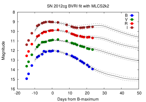
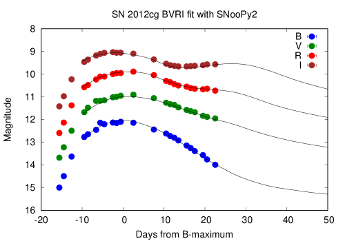
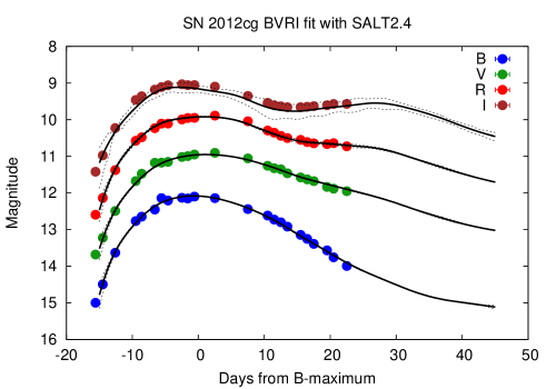
Figure 1: The fitting of SN 2012cg light curves, after correcting for Milky Way extinction. Top: MLCS2k2 templates; middle: SNooPy2 templates; bottom: SALT2.4 templates. Dashed and dotted lines represent the template uncertainties for MLCS2k2 and SALT2.4, respectively.

While applying SNooPy2, we adopted the default “EBV-model” as a proxy for a SN Ia LC:

$$m_{X}(\varphi)~{}=~{}T_{Y}+M_{Y}+\mu_{0}+K_{XY}+$$

$$R_{X}E(B-V)_{MW}+R_{Y}E(B-V)_{host},$$ (4)

where $X,Y$ denote the filter of the observed data and the template light curve, respectively, $m_{X}(\varphi)$ is the observed LC in filter $X$, $T_{Y}(\varphi,{\Delta}m_{15})$ is the template LC as a function of time, ${\Delta}m_{15}$ is the generalized decline-rate parameter associated with the ${\Delta}m_{15}(B)$ parameter by Phillips (1993), $M_{Y}({\Delta}m_{15})$ is the absolute magnitude of the SN in filter $Y$ as a function of ${\Delta}m_{15}$, $\mu_{0}$ is the reddening-free distance modulus in magnitudes, $E(B-V)$ is the color excess due to interstellar extinction either in the Milky Way (“MW”), or in the host galaxy, $R_{X,Y}$ are the reddening slopes in filter $X$ or $Y$ and $K_{XY}(t,z)$ is the cross-band K-correction that matches the observed broad-band magnitudes of a redshifted ($z\gtrsim 0.01$) SN taken with filter $X$ to a template SN LC in filter $Y$. Since all our SNe had very low redshift ($z<0.01$) we always set $X=Y$ and neglected the K-corrections, which greatly simplified the analysis of those objects.

SNooPy2 offers two sets of templates which cover different filter bands. We utilized the Prieto-templates (Prieto et al., 2006) for fitting the $BVRI$ LCs, while for the $g^{\prime}r^{\prime}i^{\prime}z^{\prime}$ data we selected the built-in CSP-templates which include the $g$-, $r$- and $i$-bands. For SN 2012cg, 2012ht and 2013dy we adopted the standard $R_{V}=3.1$ reddening slope (corresponding to the calibration=2 mode in SNooPy2), while for SN 2014J, which suffered from strong non-standard reddening, we tested both the $R_{V}\sim 1.0$ (calibration=6) and $R_{V}\sim 1.5$ (calibration=3) settings. These different calibrations are detailed in Folatelli et al. (2010).

All of these codes fit the template LCs to the observed ones via $\chi^{2}$-minimization, taking into account photometric errors as inverse weights. The optimized parameters are as follows:

• $T_{max}$: the moment of maximum light in the $B$-band (MJD)

• $A_{V}^{host}$: the interstellar extinction in the host galaxy in $V$-band (magnitude)

• $\mu_{0}$: extinction-free distance modulus (magnitude)

• $\Delta$: light curve shape parameter (MLCS2k2)

• $\Delta m_{15}$: light curve shape parameter (SNooPy2)

• $m_{B}$: peak brightness in $B$-band (SALT2, magnitude)

• $x_{0}$: light curve normalization parameter (SALT2)

• $x_{1}$: light curve shape parameter (SALT2)

• $C$: color parameter (SALT2)

Uncertainties of the fitting parameters were calculated via the standard analysis of the Hessian matrix of the $\chi^{2}$-hypersurface.

A particularly important goal of this study was checking the consistency of the distance moduli obtained from different photometric systems, i.e. to cross-compare the results from Johnson-Cousins $BVRI$ and Sloan $g^{\prime}r^{\prime}i^{\prime}z^{\prime}$. SALT2 and SNooPy2 are capable of handling LCs taken in $g^{\prime}r^{\prime}i^{\prime}$ bands, but not in the $z^{\prime}$-band. The publicly released version of MLCS2k2 contains only templates in $UBVRI$-bands. In order to make the analysis as complete as possible, we migrated the MLCS2k2 $UBVRI$ templates to cover the $g^{\prime}r^{\prime}i^{\prime}z^{\prime}$ filters. Details on this step are given in the Appendix.

Several studies (e.g. Hicken et al., 2009; Kelly et al., 2010; Lampeitl et al., 2010; Sullivan et al., 2010) pointed out the correlation between SN Ia peak brightnesses and host galaxy stellar masses: SNe in more massive ($M_{stellar}\gtrsim 10^{10}$ $M_{\odot}$) galaxies tend to be slightly brighter at peak compared to SNe in less massive hosts. We discuss the implication of this correlation on the derived distances in Section 4.

Previously the comparison of MLCS2k2 and SALT2 was presented by Kessler et al. (2009), who analyzed the first-season data from the SDSS-II SN survey. They found moderate disagreement (at the $\sim 0.1$ – $0.2$ mag level) between the distance moduli for their nearby SN sample calculated by the two codes. A similar result was obtained by Vinkó et al. (2012) when fitting the $BVRI$ data for the extremely well-observed SN 2011fe: the distance moduli given by MLCS2k2 and SALT2 differ by $\sim 0.16$ mag. In the rest of the paper we make a similar comparison for our SN sample by involving SNooPy2 and using data taken in different photometric systems.

We would like to emphasize that it is not intended to judge which code is superior over the others. We use these codes “as is” without any attempts to fine-tune or retrain their calibrations to get better match with any particular data, except for bringing them onto the same distance scale (see below).

4 Results

This section summarizes the fits obtained from the different methods, and compare the results with those from previous studies, where applicable. Note that the different methods use different Hubble-parameters ($H_{0}$) for their relative distance scales: MLCS2k2, SNooPy2 and SALT2.4 assume $H_{0}=65$, 72 and 68 km s^-1 Mpc^-1, respectively. In order to bring the reported distance moduli onto the same scale, all of them have been corrected to $H_{0}=73$ km s^-1 Mpc^-1 (Riess et al., 2016). The tables below contain these homogenized distance moduli. The cross-comparison of the distances obtained by these codes is further discussed in Section 5.

4.1 SN 2012cg

Table 2: Best-fit parameters for SN 2012cg

Parameter	Value	Error
MLCS2k2	$BVRI$
$R_{V}$	3.1	fixed
$T_{max}$ (MJD)	56081.5	0.30
$A_{V}^{host}$ (mag)	0.43	0.05
$\Delta$ (mag)	-0.19	0.07
$\mu_{0}$ (mag)	30.87	0.05
$\chi^{2}$/d.o.f.	1.09
SNooPy2	$BVRI$
$R_{V}$	3.1	fixed
$T_{max}$ (MJD)	56082.30	0.08
$A_{V}^{host}$ (mag)	0.46	0.02
$\Delta m_{15}$ (mag)	0.97	0.01
$\mu_{0}$ (mag)	30.77	0.02
$\chi^{2}$/d.o.f.	0.93
SALT2.4	$BVRI$
$T_{max}$ (MJD)	56082.39	0.05
$C$	0.08	0.02
$x_{0}$	0.28	0.01
$x_{1}$	0.45	0.04
$m_{B}$ (mag)	12.01	0.03
$\mu_{0}$ (mag)	30.85	0.09
$\chi^{2}$/d.o.f.	1.44

Previous photometry of SN 2012cg has been presented and analyzed by Silverman et al. (2012), Munari et al. (2013), Amanullah et al. (2015) and Marion et al. (2015b). Table 2 lists the optimum parameters found by the different LC fitters applied by us. Comparing their values with the ones given by the previous studies, it is seen that they are generally consistent. There is only a slight tension between the estimated values of the extinction within the host: the results in Table 2 imply $E(B-V)_{host}=A_{V}^{host}/R_{V}=0.14\pm 0.02$ mag, while Silverman et al. (2012) and Marion et al. (2015b) obtained $E(B-V)_{host}\sim 0.18\pm 0.05$ mag which is marginally consistent with our results. Our lower reddening/extinction is closer to $E(B-V)_{host}\sim 0.13$ mag estimated by Amanullah et al. (2015). For the distance modulus, the parameter that we focus on in this work, Munari et al. (2013) obtained $\mu_{0}=30.95$ assuming $E(B-V)=0.18$ mag, which, after correcting to $E(B-V)=0.14$ mag, corresponds to $\mu_{0}=30.83$ in very good agreement with our results presented in Table 2.

The light curves of SN 2012cg are plotted together with the models from the different LC fitters in Fig. 1.

4.2 SN 2012ht

Table 3: Best-fit parameters for SN 2012ht

Parameter	Value	Error	Value	Error
MLCS2k2	$BVRI$		$griz$
$R_{V}$	3.1	fixed	3.1	fixed
$T_{max}$ (MJD)	56295.1	0.30	56295.10	0.30
$A_{V}^{host}$ (mag)	0.00	0.04	0.00	0.16
$\Delta$ (mag)	0.24	0.04	0.28	0.12
$\mu_{0}$ (mag)	32.16	0.04	32.11	0.14
$\chi^{2}$/d.o.f.	0.91		1.73
SNooPy2	$BVRI$		$gri$
$R_{V}$	3.1	fixed	3.1	fixed
$T_{max}$ (MJD)	56295.23	0.08	56295.00	0.21
$A_{V}^{host}$ (mag)	0.00	0.01	0.00	0.01
$\Delta m_{15}$ (mag)	1.30	0.01	1.17	0.01
$\mu_{0}$ (mag)	32.26	0.02	32.44	0.02
$\chi^{2}$/d.o.f.	0.58		1.16
SALT2.4	$BVRI$		$gri$
$T_{max}$ (MJD)	56295.47	0.07	56295.50	0.30
$C$	-0.08	0.03	-0.14	0.05
$x_{0}$	0.111	0.003	0.116	0.007
$x_{1}$	-1.25	0.05	-0.81	0.26
$m_{B}$ (mag)	13.02	0.03	12.98	0.07
$\mu_{0}$ (mag)	32.12	0.09	32.32	0.17
$\chi^{2}$/d.o.f.	1.47		2.02

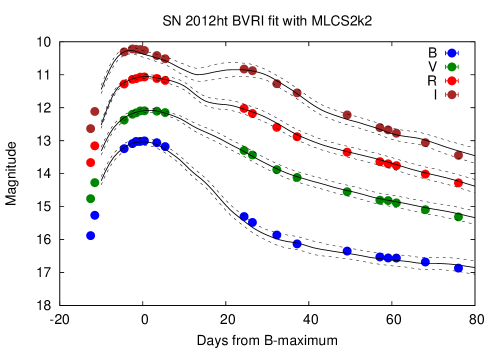
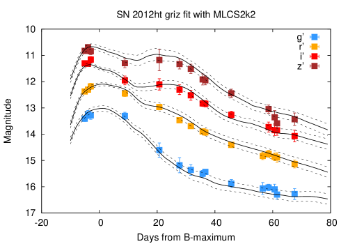
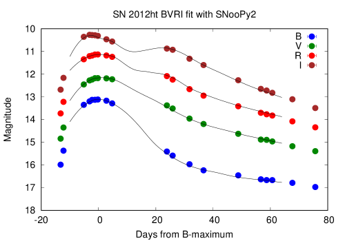
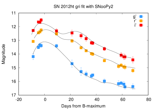
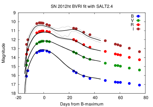
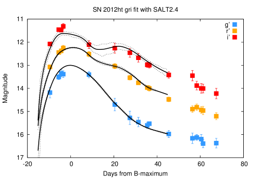
Figure 2: The fitting of the light curves of SN 2012ht, after correcting for Milky Way extinction. Top row: MLCS2k2; middle row: SNooPy2; bottom row: SALT2.4; left column: $BVRI$ data; right column: $g^{\prime}r^{\prime}i^{\prime}z^{\prime}$ data.

A photometric study of SN 2012ht has been presented by Yamanaka et al. (2014). From their $BVRI$ photometry they have estimated the following parameters: $T_{max}(B)=56295.6\pm 0.6$, $\Delta m_{15}(B)=1.39$ mag and $E(B-V)_{host}\sim 0$ mag. As seen from Table 3, these are in good agreement with our results. The light curves together with the best-fit models can be found in Fig. 2. It is seen that the $BVRI$ data that have lower measurement errors could be fit better: their reduced $\chi^{2}$ values (Table 3) are lower than those of the $g^{\prime}r^{\prime}i^{\prime}z^{\prime}$ data.

In order to test the consistency of the photometric calibration of our $BVRI$ and $g^{\prime}r^{\prime}i^{\prime}$ data, simultaneous fits to the combined LCs were also computed with SNooPy2 and SALT2.4 (MLCS2k2 was trained only on $BVRI$ data, so that code was not applied in this test). As expected, these fits produced slightly higher $\chi^{2}$ values than the fits to the $BVRI$ LCs alone, but their best-fit parameters were consistent with the ones listed in Table 3. In particular, the distance modulus from the combined fits turned out to be $\mu_{0}=32.20\pm 0.01$ mag ($\chi^{2}$/d.o.f=0.83) from SNooPy2, while from SALT2.4 it is $32.13\pm 0.08$ mag ($\chi^{2}$/d.o.f.=2.81). These parameters are closer to those obtained from fitting the $BVRI$ LCs than those from fitting the $g^{\prime}r^{\prime}i^{\prime}z^{\prime}$ data, probably because of the lower measurement uncertainties of the former.

4.3 SN 2013dy

Table 4: Best-fit parameters for SN 2013dy

Parameter	Value	Error	Value	Error
MLCS2k2	$BVRI$		$griz$
$R_{V}$	3.1	fixed	3.1	fixed
$T_{max}$ (MJD)	56500.20	0.30	56500.20	0.30
$A_{V}^{host}$ (mag)	0.48	0.06	0.28	0.16
$\Delta$ (mag)	-0.23	0.06	-0.30	0.12
$\mu_{0}$ (mag)	31.51	0.06	31.65	0.13
$\chi^{2}$/d.o.f.	1.34		1.91
SNooPy2	$BVRI$		$gri$
$R_{V}$	3.1	fixed	3.1	fixed
$T_{max}$ (MJD)	56501.30	0.08	56501.03	0.15
$A_{V}^{host}$ (mag)	0.40	0.02	0.61	0.05
$\Delta m_{15}$ (mag)	0.96	0.01	0.80	0.01
$\mu_{0}$ (mag)	31.52	0.03	31.44	0.04
$\chi^{2}$/d.o.f.	0.99		3.45
SALT2.4	$BVRI$		$gri$
$T_{max}$ (MJD)	56501.44	0.06	56501.99	0.14
$C$	0.089	0.025	0.03	0.03
$x_{0}$	0.154	0.004	0.169	0.006
$x_{1}$	0.695	0.044	1.51	0.12
$m_{B}$ (mag)	12.67	0.03	12.57	0.04
$\mu_{0}$ (mag)	31.52	0.09	31.72	0.11
$\chi^{2}$/d.o.f.	0.76		2.70

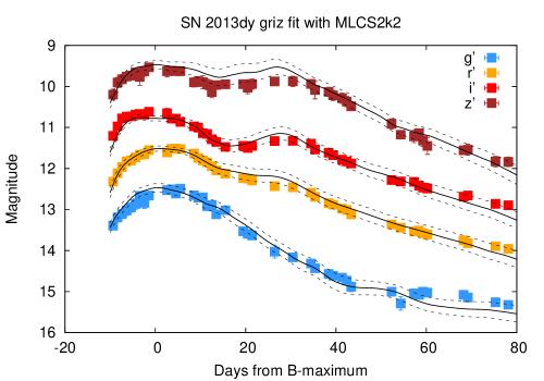
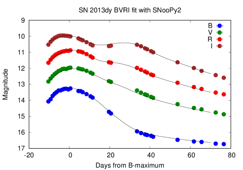
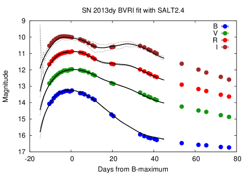
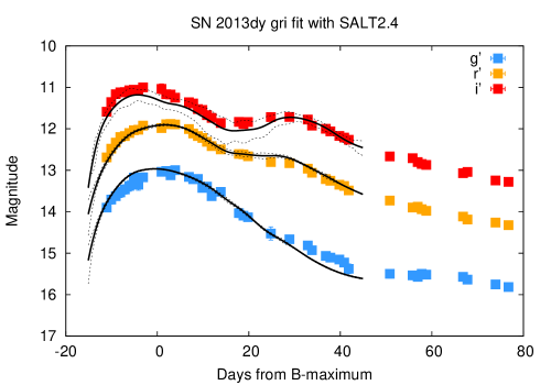
Figure 3: The same as Fig.2 but for SN 2013dy.

Light curves of SN 2013dy have been published recently by Pan et al. (2015) (P15) and Zhai et al. (2016) (Z16) in the $BVRIriZYJH$ and $UBVRI$ bands, respectively. Zhai et al. (2016) also presented photometry obtained by Swift/UVOT.

Pan et al. (2015) applied the SNooPy2 code to fit their full $BVRIriZYJH$ dataset simultaneously, and obtained $T_{max}(B)=56501.1$, $\Delta m_{15}=0.886\pm 0.006$, $E(B-V)_{host}=0.206\pm 0.005$ mag and $\mu_{0}=31.49\pm 0.01$ mag. Comparing these values with those in Table 4 it is apparent that the results of Pan et al. (2015) are close to the ones obtained in the present study, although the differences somewhat exceed the formal errors given by SNooPy2. Comparing the best-fit values of the common parameters obtained from different methods, e.g. $A_{V}^{host}$ or $\mu_{0}$, it is seen that they also deviate much more than the uncertainties given by the codes. Thus, it is suspected that the formal parameter errors, especially those reported by SNooPy2, are underestimated, and the true uncertainties should be higher. Keeping this in mind, the solutions presented in Table 4 are entirely consistent with the LC fit given by Pan et al. (2015). The fit of the model LCs to the data can be seen in Fig. 3.

Table 5: Cross-comparison of the parameters from fitting independent data on SN 2013dy. Uncertainties are in parentheses.

Parameter	this work	P15	Z16
MLCS2k2:
$T_{max}$	56500.2 (0.3)	56500.5 (0.3)	56501.4 (0.3)
$A_{V}^{host}$	0.48 (0.06)	0.42 (0.07)	0.45 (0.06)
$\Delta$	$-0.23$ (0.06)	$-0.20$ (0.05)	$-0.22$ (0.05)
$\mu_{0}$	31.51 (0.06)	31.53 (0.06)	31.53 (0.07)
SNooPy2:
$T_{max}$	56501.30 (0.08)	56501.48 (0.11)	56501.29 (0.11)
$A_{V}^{host}$	0.40 (0.02)	0.31 (0.02)	0.43 (0.02)
$\Delta m_{15}$	0.96 (0.01)	0.97 (0.02)	0.86 (0.02)
$\mu_{0}$	31.52 (0.03)	31.56 (0.01)	31.52 (0.02)
SALT2.4:
$T_{max}$	56501.44 (0.06)	56501.47 (0.04)	56502.09 (0.14)
$C$	0.089 (0.025)	0.081 (0.016)	0.149 (0.024)
$x_{0}$	0.154 (0.004)	0.152 (0.003)	0.143 (0.004)
$x_{1}$	0.695 (0.044)	0.814 (0.044)	1.002 (0.073)
$m_{B}$	12.670 (0.028)	12.682 (0.025)	12.743 (0.028)
$\mu_{0}$	31.52 (0.08)	31.573 (0.069)	31.450 (0.090)

We re-analyzed the $BVRI$ light curves of SN 2013dy from both Pan et al. (2015) and Zhai et al. (2016) with all three methods applied in this paper in order to cross-compare the results from fitting measurements taken independently on the same SN. We assumed $R_{V}=3.1$ for all fits, as earlier. The results are shown in Table 5. It is seen that the consistency between the distance moduli from the three methods is excellent for all data. Overall, the distance moduli from the Konkoly data differ by less than $\sim 1\sigma$ ($\lesssim 0.1$ mag) from both the P15 and Z16 results. Also, it is seen from Table 5 that similar amount of dispersion in the distance moduli derived by the different codes from the same dataset appears for the P15 and Z16 LCs as well as for our data, which suggests that this dispersion is probably not simply due to photometric calibration issues, at least for the $BVRI$ data.

In addition, we also modeled the combined $BVRI$ + $g^{\prime}r^{\prime}i$ LCs as in the case for SN 2012ht. The resulting distance moduli are $\mu_{0}=31.45\pm 0.01$ mag ($\chi^{2}$/d.o.f.=2.92) from SNooPy2 and $\mu_{0}=31.54\pm 0.07$ mag ($\chi^{2}$/d.o.f.=2.11) from SALT2.4. Again, these results are in good agreement with those listed in Table 4, even though the $\chi^{2}$ values of the combined fits are somewhat higher but still acceptable (note again that the uncertainty of $\mu_{0}$ reported by SNooPy2 is underestimated).

4.4 SN 2014J

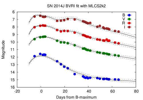
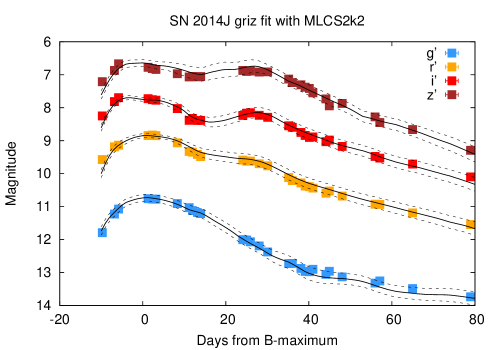
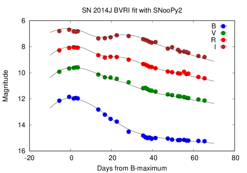
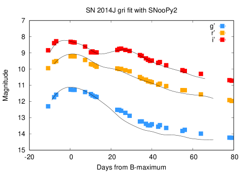
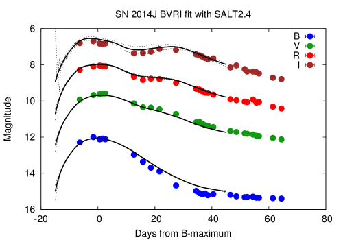
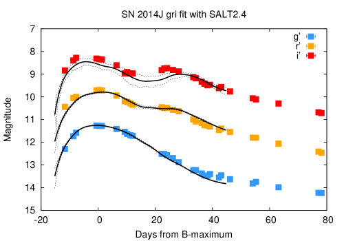
Figure 4: The same as Fig.2 but for SN 2014J.

Table 6: Best-fit parameters for SN 2014J

Parameter	Value	Error	Value	Error
MLCS2k2	$BVRI$		$griz$
$R_{V}$	1.4	fixed	1.4	fixed
$T_{max}$ (MJD)	56689.8	0.50	56689.8	0.50
$A_{V}^{host}$ (mag)	1.84	0.09	1.49	0.16
$\Delta$ (mag)	-0.13	0.08	-0.24	0.12
$\mu_{0}$ (mag)	27.72	0.09	27.99	0.13
$\chi^{2}$/d.o.f.	3.62		2.37
$R_{V}$	1.0	fixed	1.0	fixed
$T_{max}$ (MJD)	56689.8	0.50	56689.8	0.50
$A_{V}^{host}$ (mag)	1.41	0.08	1.16	0.16
$\Delta$ (mag)	-0.16	0.07	-0.25	0.12
$\mu_{0}$ (mag)	28.14	0.08	28.21	0.13
$\chi^{2}$/d.o.f.	3.15		2.32
SNooPy2	$BVRI$		$gri$
$R_{V}$	1.5	fixed	1.5	fixed
$T_{max}$ (MJD)	56689.99	0.42	56690.86	0.24
$A_{V}^{host}$ (mag)	1.89	0.05	1.40	0.03
$\Delta m_{15}$ (mag)	1.04	0.04	1.05	0.03
$\mu_{0}$ (mag)	27.50	0.02	27.69	0.05
$\chi^{2}$/d.o.f.	4.21		16.73
$R_{V}$	1.0	fixed	1.0	fixed
$T_{max}$ (MJD)	56689.99	0.34	56690.86	0.24
$A_{V}^{host}$ (mag)	1.34	0.03	0.98	0.02
$\Delta m_{15}$ (mag)	1.04	0.04	1.06	0.03
$\mu_{0}$ (mag)	27.99	0.02	28.01	0.05
$\chi^{2}$/d.o.f.	2.99		17.13
SALT2.4	$BVRI$		$gri$
$T_{max}$ (MJD)	56690.88	0.11	56691.49	0.11
$C$	1.22	0.03	0.86	0.03
$x_{0}$	0.416	0.013	0.544	0.017
$x_{1}$	0.03	0.06	1.39	0.07
$m_{B}$ (mag)	11.50	0.03	11.25	0.03
$\mu_{0}$ (mag)	26.74	0.13	27.80	0.12
$\chi^{2}$/d.o.f.	5.83		5.87

As seen in Table 6, the LCs of SN 2014J have been fit with two different models assuming different reddening laws for the host galaxy in MLCS2k2 and SNooPy2. This was motivated by the fact that many studies (see below) found $R_{V}<2$ in M82, quite different from the Milky Way value of $R_{V}=3.1$.

When using MLCS2k2, we considered two different scenarios: first, we adopted $A_{V}^{MW}=0.43$ mag from the extinction map of Schlafly & Finkbeiner (2011) at the position of SN 2014J, and $R_{V}=1.4$ based on the results of Goobar et al. (2014), Foley et al. (2014) and Amanullah et al. (2014). Secondly, we let $R_{V}$ float until the lowest $\chi^{2}$ was found by MLCS2k2. This resulted in $R_{V}\sim 1.0$, and the parameters corresponding to this solution are adopted as the best-fit MLCS2k2 values (see Table 6). Note that such a low value of $R_{V}$ is close to the limiting case of Rayleigh scattering from very small particles, producing $R_{V}\sim 1.2$ (Draine, 2003). From the full sample of the SDSS-II SN survey (361 SNe Ia) Lampeitl et al. (2010) found that the average extinction law for SNe in passive host galaxies is $R_{V}=1.0\pm 0.2$. Thus, even though the host of SN 2014J, M82, is an extremely active star-forming galaxy, such a low value for the extinction law is not unprecedented.

In SNooPy2, different reddening laws are implemented as different “calibrations” (Burns et al., 2014). We applied both the calibration=3 and calibration=6 settings (corresponding to $R_{V}\sim 1.5$ and $R_{V}\sim 1.0$, respectively), and list the best-fit parameters for each in Table 6.

Note that Marion et al. (2015a) adopted a different Milky Way extinction value toward SN 2014J (they used $E(B-V)_{MW}=0.05$ mag corresponding to $A_{V}^{MW}=0.16$ mag), because the dust content of M82 may influence the far-IR maps of Schlafly & Finkbeiner (2011) in that direction. Using this lower Milky Way extinction parameter one would get $\sim 0.1$ mag higher $A_{V}^{host}$ and $\sim 0.15$ mag higher distance modulus for SN 2014J. While keeping this in mind, in the following we use the higher Milky Way extinction value as given by the reddening maps of Schlafly & Finkbeiner (2011). In this case the MLCS2k2 results are directly comparable to the ones derived by SNooPy2, because SNooPy2 automatically applies the Schlafly & Finkbeiner (2011) values for calculating the Milky Way extinction.

SALT2.4 fits the reddening of the SN in a different way: instead of applying the same dust extinction law as MLCS2k2 or SNooPy2, it models the reddening via the $C$ color parameter (see Eq.2). Thus, the effect of the strong interstellar extinction on the LCs of SN 2014J is reflected by the extremely large value of its SALT2.4 color coefficient, which is more than an order of magnitude higher than for the other three SNe.

The light curves are plotted in Fig. 4.

Applying SNooPy2 on their own $UBVRIJHK$ photometry, Marion et al. (2015a) obtained $T_{max}(B)=56689.74\pm 0.13$ MJD, $dm_{15}(B)=1.11\pm 0.02$, $E(B-V)_{host}=1.23\pm 0.01$ and $\mu_{0}=27.85\pm 0.09$ mag in calibration=4 mode ($R_{V}\sim 1.46$). Their reddening value, $E(B-V)_{host}$, implies $A_{V}^{host}=1.80\pm 0.03$ mag. These parameters are marginally consistent with our results listed in Table 6. However, the relatively large differences between the distance moduli obtained from the $BVRI$ and $griz$ data, and also between the results from MLCS2k2 and SNooPy2, suggest that the $R_{V}\sim 1.4$ solution may not be the best one as far as LC fitting is concerned. Indeed, by comparing the distance moduli obtained from the $R_{V}\sim 1.0$ solutions, it seems that those values are more consistent with each other. The average $\mu_{0}$ for the latter solution is $\sim 28.09\pm 0.11$ mag, while it is $\sim 27.72\pm 0.20$ mag for the $R_{V}\sim 1.4$ solution. The dispersion of the distance moduli derived from the two sets of light curves and two independent codes is much less when $R_{V}=1.0$ is used for the M82 reddening law, compared to the $R_{V}\sim 1.4$ case adopted by Marion et al. (2015a).

Fitting the combined $BVRI$ + $g^{\prime}r^{\prime}i^{\prime}$ dataset with SNooPy2 gave distance moduli similar to those listed in Table 6: $\mu_{0}=27.50\pm 0.02$ (calibration=3) and $\mu_{0}=28.02\pm 0.02$ (calibration=6). However, the reduced $\chi^{2}$ values for the combined fits were $31.66$ and $34.79$, respectively, indicating poor fitting quality. Comparing the best-fit template LCs with the observed ones revealed that the $g^{\prime}$ band data could not be fit simultaneously with the other bands: while the shape of the template LC was similar to the observed one, the observed $g^{\prime}$-band LC was too bright (by $\sim 0.5$ mag) with respect to the template. This could be due to either an issue with our photometry (which is unlikely given that the other data do not show such a high deviation), or the complexity of the reddening law in M82 that may not be fully modeled by a single $R_{V}$ (Foley et al., 2014).

The SALT2.4 code could not provide reliable distances for this heavily reddened SN. The SALT2.4 distances for SN 2014J are inconsistent with each other, as well as with the distances given by the other two codes. SALT2.4 also failed to give consistent fits to the combined $BVRI$+$g^{\prime}r^{\prime}i^{\prime}$ LCs: neither of the templates matched the observed data adequately, resulting in $\chi^{2}>50$.

We conclude that for SN 2014J only MLCS2k2 and SNooPy2 were able to provide more-or-less consistent distances, and both of those LC fitters suggest $R_{V}\sim 1.0$, i.e. a lower value than found by the spectroscopic studies. However, the failure of the simultaneous fitting of the combined LCs suggest that the complexity of the extinction within M82 may affect the derived distances to SN 2014J more than in the other three cases.

4.5 Correction for the host galaxy mass

Table 7: Differences in distance moduli after corrections for host galaxy masses

SN	SALT$-$MLCS	SALT$-$MLCS	SALT$-$SNooPy	SALT$-$SNooPy
	$BVRI$ (mag)	$g^{\prime}r^{\prime}i^{\prime}z^{\prime}$ (mag)	$BVRI$ (mag)	$g^{\prime}r^{\prime}i^{\prime}$ (mag)
2012cg	0.01 ($-0.02$)	–	0.11 (0.08)	–
2012ht	$-0.01$ ($-0.04$)	0.24 (0.21)	$-0.11$ ($-0.14$)	$-0.09$ ($-0.12$)
2013dy	0.04 (0.01)	0.1 (0.07)	0.03 (0.00)	0.31 (0.28)

The distance moduli given in Tables 2-6 do not contain the correction for the host galaxy mass (see Section 1 for references). Betoule et al. (2014) found that SNe Ia that exploded in host galaxies having total stellar mass of $M_{stellar}>10^{10}$ $M_{\odot}$ are $\sim 0.06$ mag brighter than those in less massive hosts. The calibration of SALT2.4 by Betoule et al. (2014) that we applied in this paper already contains this so-called “mass-step”: the $M_{B}$ parameter given after Eq.3 is valid for SNe in less massive hosts, and it is $M_{B}-0.061$ mag for SNe in more massive hosts.

The stellar masses for the host galaxies in this paper are listed in Table 1. These were derived, following Pan et al. (2014), by applying Z-PEG (Le Borgne & Rocca-Volmerange, 2002) to the observed galaxy SEDs (see Table 1 for references). It is seen that only SN 2014J is affected by this correction, since the hosts of the other three SNe are below $\log M_{stellar}=10$. Thus, their $M_{B}$ parameter does not need to be corrected, and their SALT2.4 distances are final. Unfortunately, the SALT2.4 distance moduli of SN 2014J are unreliable as they are affected by the strong non-standard interstellar extinction (see the previous subsection). These systematic uncertainties ($\gtrsim 0.5$ mag; Table 6) are much higher than the correction for the host galaxy mass ($\sim 0.06$ mag) in the case of SN 2014J.

Nevertheless, we investigated whether the mass-step correction could bring the derived distances to better agreement with each other for the other three SNe. Since neither MLCS2k2, nor SNooPy2 contain the mass-step correction in their calibrations, we followed the practice applied by Riess et al. (2016) by adding $0.03$ mag to the MLCS2k2/SNooPy2 distance moduli of SN 2014J and subtracting $0.03$ mag from the distances of SNe 2012cg, 2012ht and 2013dy, thus, mimicking the existence of the mass-step in their peak brightnesses.

Table 7 shows the differences between the distance moduli estimated by SALT2.4 and the other two codes for both photometric systems after implementing the host mass correction as described above. For comparison, we give the same differences between the uncorrected distances in parentheses. Ideally, after correction all these differences should be zero. In reality, it is apparent that the effect of the host mass correction is minimal: sometimes it makes the agreement slightly better, sometimes slightly worse, but its amount ($\pm 0.03$ mag) is an order of magnitude less than the differences between the distance moduli given by the different LC-fitting codes.

It is concluded that the host mass correction on the distance modulus is negligible compared to the other sources of uncertainty, at least for the SNe studied in this paper. Note, however, that in studies using relative distances, such as Betoule et al. (2014); Riess et al. (2016) and others, this effect can be much more important and significant. Therefore, in the rest of the paper we use the uncorrected distances (i.e. without the mass-step) as given in Tables 2-6, but note that it is desirable to include the host mass correction in future retraining of the MLCS2k2 and/or SNooPy2 templates.

5 Discussion

In this section we cross-compare the parameters derived by the three independent codes, and check the consistency between the values inferred from different photometric systems ($BVRI$ vs $griz$) and by different LC fitters.

5.1 Time of maximum light

For Type Ia SNe the moment of maximum light in the $B$-band has been used traditionally as the zero-point of time. At first it seems to be fairly easy to measure directly from the data, at least when the LC in $B$-band is available. From Tables 2 - 6 it is seen that the LC fitters used in this study do a good job in estimating $T_{max}(B)$ even if the $B$-band LC is not included in the fitting. The consistency between the derived values is also relatively good: the dispersion around the mean values is 0.49, 0.21, 0.71 and 0.67 day for SN 2012cg, 2012ht, 2013dy and 2014J, respectively. Note, however, that SALT2.4 gets later maximum times systematically by $\Delta t>0.5$ day relative to MLCS2k2, similar to the finding by Vinkó et al. (2012) and Pereira et al. (2013) for SN 2011fe.

5.2 Extinction

Figure 5: The narrow NaD features in the high-resolution spectrum of SN 2012ht taken at $11$ days before maximum (left panel) and 2013dy at $12$ days after maximum (right panel). The components from the Milky Way and host galaxy are labeled. See text for details.

The host galaxy dust extinction parameters ($A_{V}^{host}$) in Tables 2 - 6 look generally consistent with each other. The match between the values provided by the same code for $BVRI$ and $griz$ is usually better than the agreement between the results of the different codes (here only MLCS2k2 and SNooPy2 are relevant, because SALT2.4 does not model dust extinction).

As an independent sanity check, we compare the average $A_{V}^{host}$ values from MLCS2k2 and SNooPy2 for SN 2012ht and 2013dy with high-resolution spectra obtained with the Hobby-Eberly Telescope (HET). For SN 2013dy these spectra were published by Pan et al. (2015), while those for SN 2012ht are yet unpublished. In Fig. 5 the spectral regions containing the Na D ($\lambda\lambda$5890,5896) doublet are shown. The narrow Na D features originating from the ISM both in the Milky Way and in the host galaxy (separated by the Doppler-shift due to the recession velocity of the host) are labeled. The strength of the Na D doublet is thought to be proportional to the amount of extinction, at least as a first approximation (Richmond et al., 1994; Poznanski et al., 2012). It is seen that the dust extinction within the host galaxy for SN 2012ht is negligible (no narrow Na D absorption is visible at the redshift of the host) compared to the Milky Way component. This is in excellent agreement with the predictions from the LC fitters, because both codes resulted in $A_{V}^{host}=0$ magnitude for SN 2012ht.

Concerning SN 2013dy, the consistency between the photometric and spectroscopic extinction estimates is also very good. In Fig. 5 the Na D profiles in the host galaxy have approximately the same strength as the Milky Way components. From Tables 1 and 4, $A_{V}^{MW}=0.42$ mag and $A_{V}^{host}\sim 0.44\pm 0.14$ mag were taken for SN 2013dy, which are, again, in good agreement with the relative strengths of the Na D profiles in the high-resolution spectra.

The case of SN 2014J is more problematic, as this SN occured within a host galaxy that has a known complex dust content. Foley et al. (2014) presented an in-depth study of the wavelength-dependent reddening and extinction toward SN 2014J, and concluded that it is probably much more complex than a simple extinction law parametrized by a single value of $A_{V}$ and $R_{V}$. Keeping this in mind, it is not surprising that the LC-fitting codes applied in this paper failed to produce consistent results with the spectroscopic estimates (Amanullah et al., 2014; Foley et al., 2014; Goobar et al., 2014; Brown et al., 2015; Gao et al., 2015) that all found $R_{V}\gtrsim 1.4$.

5.3 Light curve shape/stretch parameter

Table 8:

SN	$\Delta m_{15}(B)$	$\Delta m_{15}(B)$	$\Delta m_{15}(B)$
	$BVRI$ (mag)	$g^{\prime}r^{\prime}i^{\prime}z^{\prime}$ (mag)	combined (mag)
2012cg	0.984 (0.041)	–	–
2012ht	1.275 (0.045)	1.217 (0.041)	1.298 (0.010)
2013dy	0.960 (0.043)	0.858 (0.015)	0.971 (0.007)
2014J	1.034 (0.065)	0.952 (0.105)	0.981 (0.074)

The light curve shape/stretch parameter is the one that is most strongly connected to the peak brightness of a Type Ia SN; thus, it has a direct influence on the distance measurement. Since the three LC-fitting codes adopt slightly different parametrizations of the light curve shape, we converted each of them to the traditional $\Delta m_{15}(B)$ (Phillips, 1993). From the MLCS2k2 templates we get $\Delta m_{15}(B)~{}=~{}1.07~{}+~{}0.67\cdot\Delta~{}-~{}0.10\cdot\Delta^{2}$. For SNooPy2 we adopted $\Delta m_{15}(B)~{}=~{}0.13~{}+~{}0.89\cdot\Delta m_{15}$ (Burns et al., 2011), while for SALT2.4 we used $\Delta m_{15}(B)~{}=~{}1.09-0.161\cdot x_{1}+0.013\cdot x_{1}^{2}-0.0013\cdot x_{1}^{3}$ (Guy et al., 2007).

Table 8 lists the resulting $\Delta m_{15}(B)$ values, averaged over the three methods, for the $BVRI$ and $g^{\prime}r^{\prime}i^{\prime}z^{\prime}$ data and for the combined fits, respectively. It is seen that the fits to the $g^{\prime}r^{\prime}i^{\prime}z^{\prime}$ data alone tend to result in systematically lower decline rates than the fits to the $BVRI$ data or the combined $BVRI$+$g^{\prime}r^{\prime}i^{\prime}$ data. The deviation is the highest in the case of SN 2013dy, $\sim 0.1$ mag, and it is lower for the other two SNe. Neglecting the differences between the other fitting parameters, an underestimate of the decline rate by $\sim 0.1$ mag would cause an overestimate of $\sim 0.08$ mag in the distance modulus (applying the decline rate - absolute peak magnitude calibration by Burns et al. (2014)). Since the derived distance moduli do not show such a systematic trend between the $BVRI$ and $g^{\prime}r^{\prime}i^{\prime}z^{\prime}$ data, and the differences between them are sometimes higher than 0.08 mag (see next section), it is concluded that the systematic underestimate of the decline rates from our $g^{\prime}r^{\prime}i^{\prime}z^{\prime}$ photometry is not significant, at least from the present dataset. The number of SNe in this paper is too low to draw more definite conclusions on the cause of the dependence of the light curve shape/stretch parameter on the photometric bands (whether it is merely due to uncertainties in the data or might have physical origin), but it would be worth studying on a larger sample of SNe.

5.4 Distance

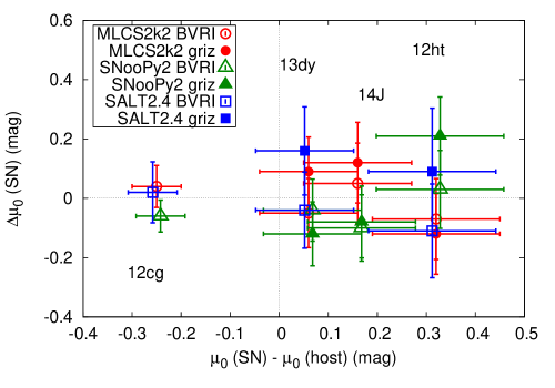
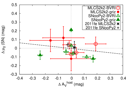
Figure 6: Left panel: Residual distance moduli from their mean value for each SNe. Different symbols denote the different LC-fitting codes, as explained in the legend. Right panel: the distance modulus residuals as a function of the dust extinction residuals. The dashed line indicates a simple linear fit to these data. See text for explanation.

Table 9: Final absolute distances to SNe Ia

SN	$\mu_{0}$(SN)	$\mu_{0}$(host)	$D_{SN}$	$D_{host}$	Difference
	(mag)	(mag)	(Mpc)	(Mpc)	(mag)
2011fe	29.13 $\pm 0.08$	29.13 $\pm 0.04$	$6.7^{+0.3}_{-0.2}$	$6.7^{0.1}_{0.1}$	0.00 ($<1\sigma$)
2012cg	30.83 $\pm$0.05	31.08 $\pm$0.29	$14.6^{+0.3}_{-0.3}$	$16.44^{+2.4}_{-2.1}$	$-0.25$ ($\lesssim 1\sigma$)
2012ht	32.23 $\pm$0.13	31.91 $\pm$0.04	$27.9^{+1.7}_{-1.6}$	$24.1^{+0.5}_{-0.5}$	0.32 ($\sim 2.3\sigma$)
2013dy	31.54 $\pm$0.08	31.50 $\pm$0.08	$20.3^{+0.8}_{-0.7}$	$20.0^{+0.8}_{-0.7}$	0.04 ($\lesssim 1\sigma$)
2014J	28.09 $\pm$0.11	27.93 $\pm$0.35	$4.1^{+0.2}_{-0.2}$	$3.9^{+0.7}_{-0.6}$	0.16 ($\lesssim 1\sigma$)

Distance is one of the most important outputs of the LC fitting codes under study. Cross-comparing the distance estimates produced by the various codes may reveal important constraints on the systematics that are present either in the basic assumptions of the methods or in their implementation and calibrations.

For the extremely well-observed SN 2011fe, Vinkó et al. (2012) found a $0.16\pm 0.07$ mag systematic difference ($\sim 2\sigma$) between the distance moduli provided by MLCS2k2 and SALT2, when applied for the same homogeneous photometric data. In the left panel of Fig. 6 we plot the residual distance moduli (i.e. the difference of the distance modulus given by the LC-fitting code for each filter set, $BVRI$ or $griz$, from the mean distance modulus) for each SNe as a function of the difference between their mean distance moduli and the ones listed in Table 1. The results from fits to $BVRI$ data are plotted with open symbols, while those from $griz$ data are shown by the filled symbols. The color and the shape of the symbols encode the fitting method as indicated by the figure legend.

From this plot it is seen that a separation of $\Delta\mu_{0}\sim 0.2$ mag can still be present between the distance moduli given by different LC-fitting codes, similar to the case of SN 2011fe, although the difference varies from SN to SN and it is less than $\sim 0.2$ mag for the majority of the cases considered in the present paper.

For the three moderately reddened SNe (2012cg, 2012ht and 2013dy) the distances given by MLCS2k2 and SALT2.4 are in remarkable agreement (their difference is $0.02$, $0.04$ and $-0.01$ mag, respectively) for the $BVRI$ data. The differences between the MLCS2k2 and SNooPy2 distances in $BVRI$ are also very good; they do not exceed $0.1$ mag. This is not true in the case of SN 2014J, as expected, because SALT2.4 could not provide reliable distances for such an extremely reddened object, thus, they are not plotted in Fig. 6. Note that this does not mean that SALT2.4 is a less reliable code. It is just the consequence of the underlying model, and the code works fine for moderately reddened SNe Ia.

The agreement is slightly worse for our $g^{\prime}r^{\prime}i^{\prime}z^{\prime}$ photometry, partly because those data have smaller signal-to-noise ratio than our $BVRI$ light curves. From these data it is found that the differences between the distance moduli provided by the three codes may differ by $\sim 0.2$ mag. A similar $\lesssim 0.2$ mag difference can be seen when comparing the distances of the same SN taken from $BVRI$ and $g^{\prime}r^{\prime}i^{\prime}z^{\prime}$ LCs: for SN 2012ht $\mu_{0}(BVRI)-\mu_{0}(g^{\prime}r^{\prime}i^{\prime}z^{\prime})$ is $0.05$, $-0.18$ and $-0.30$ mag from MLCS2k2, SNooPy2 and SALT2.4, respectively; for SN 2013dy these are $-0.14$, $0.08$ and $-0.20$; for SN 2014J $-0.07$, $-0.02$ and $-1.06$ mag. It is seen that there is no systematic trend in these numbers, which suggests that these differences are probably not due to systematic errors in the photometric calibration; more probably they represent the internal uncertainties of the template LC vectors for the different bands. Given that our data were obtained by two telescopes from two different sites (one for $BVRI$ and another one for $g^{\prime}r^{\prime}i^{\prime}z^{\prime}$), this result may also give a hint on the possible amount of systematic errors in the distance moduli when fitting inhomogeneous LCs taken by more than one telescope.

It is concluded that applying these three popular LC-fitting codes as distance calculators on homogeneous $BVRI$ photometry on nearby, moderately reddened SNe Ia one can derive consistent distances that agree with each other within $\lesssim 0.1$ mag or better. Even for strongly reddened SNe, like SN 2014J, MLCS2k2 and SNooPy2 work quite well; their distances differ by only $\sim 0.15$ mag. We found slightly larger ($\sim 0.2$ mag) differences in the distances from our $g^{\prime}r^{\prime}i^{\prime}z^{\prime}$ photometry.

In the right panel of Fig. 6 we investigate whether the differences between the distance moduli were due to systematic under- or overestimates of the extinction parameter $A_{V}^{\mathrm{h}ost}$. In this panel the same $\Delta\mu_{0}$ residuals are plotted against the residual of the host extinction parameter $\Delta A_{V}^{\mathrm{h}ost}$ (we consider only the extinction within the host here, since the Milky Way extinction was kept fixed at the values provided by the Milky Way dust maps). SN 2011fe is also plotted in this diagram (with black symbols) taking the data from Vinkó et al. (2012). Again, only the MLCS2k2 and SNooPy2 results are used.

If the expected correlation between the distances and extinction (higher extinction estimates imply shorter distances) exists, then one should see positive $\Delta\mu_{0}$ values for negative $\Delta A_{v}^{host}$ and vice versa. It is not clearly visible in Fig. 6, as most of the data scatter around 0 within $\sim 0.2$ mag in all directions. The dashed line is a simple linear fit to the data. Its slope, $-0.16\pm 0.23$, is in the expected direction of a correlation between the extinction and distance, though it is not significant. Although it is probable that our sample is too low to detect this, the lack of significant correlation suggests that the distances given by either MLCS2k2 or SNooPy2 are less affected by systematic under- or overestimates of the extinction parameter.

In Table 9 we summarize the final absolute distances for each SN studied, supplemented by the data for SN 2011fe from Vinkó et al. (2012). These are defined as the simple, unweighted mean of all distance moduli from our Konkoly + Baja data except for SN 2014J where the SALT2.4 distances were omitted due to the reason mentioned above. The Cepheid-based distances to the host galaxies (Riess et al., 2016) from Table 1 are also shown for easy comparison. In the final column the difference between the SN and host distance moduli is given with respect to their combined uncertainties $\sigma(\mu_{0})=\sqrt{\sigma^{2}_{SN}+\sigma^{2}_{host}}$. It is apparent that even though the individual SN-based mean distances are uncertain at the $\sim 0.10$ mag level, their deviations from their host galaxy distances obtained independently are less than $1\sigma$ in 4 out of 5 cases, which is encouraging. Higher deviation ($2\sigma$) is seen only in the case of SN 2012ht.

Recently Riess et al. (2016) showed that by properly combining Cepheid- and SN Ia-based distance scales, anchored to local galaxies having independent geometric distances, one can reduce the uncertainty of the local value of the Hubble-constant ($H_{0}$) to $\sim 2.4$ percent. Such an accuracy on the individual distances to local galaxies would need a $\sim 0.05$ mag dispersion in the distance moduli. Our results above show that this is still not the case for every SN at present, although the agreement between the distance moduli are close to the $\lesssim 0.05$ mag level for the best-observed SNe in our sample. The $\sim 0.1$ – 0.2 mag dispersion between the distance moduli calculated by different LC fitters is close to the $\sim 0.15$ mag dispersion found by Riess et al. (2016) when comparing their Cepheid- and SN Ia-based distances to the same galaxies.

As the sample of the SNe Ia having accurately calibrated photometry (Scolnic et al., 2015) is growing rapidly, we can expect significant improvement in the accuracy of the individual distance estimates to local galaxies in the near future. This would be an important step toward better understanding the physics of SN Ia explosions.

6 Summary

We have studied 3 public light curve fitting codes for SNe Ia by cross-comparing the time of maximum, extinction and distance parameters inferred from the light curves of 4 nearby, bright, well-observed SNe Ia (2012cg, 2012ht, 2013dy, 2014J). Our results are summarized as follows.

• The moment of $B$-band maximum can be estimated within $\pm 0.7$ day, even if there are no data observed in the $B$-band. Note that SALT2.4 tends to give systematically later maximum times by $\Delta t_{max}\sim 0.5$ day than MLCS2k2 (Vinkó et al., 2012; Pereira et al., 2013).

• For moderately reddened ($A_{V}^{host}<0.5$ mag) SNe, MLCS2k2 and SNooPy2 did quite a good job in estimating the relative amount of interstellar extinction within the host galaxy ($A_{V}^{host}$) compared to the extinction within the Milky Way ($A_{V}^{MW}$). The inferred $A_{V}^{host}/A_{V}^{MW}$ extinction ratios for SNe 2012ht and 2013dy are consistent with the relative strengths of the interstellar NaD lines from high-resolution spectroscopy. This is not the case for the heavily-reddened SN 2014J, where the light curve fitting resulted in reddening parameters having large scatter and being different from the results of spectroscopic analyses.

• Regarding the distance modulus, it is found that for the moderately reddened SNe 2012cg, 2012ht and 2013dy the consistency between the results from the three LC-fitting codes is $\lesssim 0.1$ mag for our highest quality $BVRI$ data, even without taking into account the dependence of the peak brightnesses on the host galaxy masses. This is significantly better than the $\sim 0.16$ mag difference found by Vinkó et al. (2012) for SN 2011fe. The dispersion is somewhat higher, $\sim 0.2$ mag, for our $g^{\prime}r^{\prime}i^{\prime}z^{\prime}$ LCs that have lower S/N ratio, and the same is true for the strongly reddened SN 2014J. We found a negative, though nonsignificant, distance–extinction correlation in our sample, suggesting that the distances provided by both MLCS2k2 and SNooPy2 are not strongly affected by systematic over- or underestimates of the extinction. The final distances to our sample SNe are in very good agreement with the Cepheid-based distances to their host galaxies (see Table 9). From these results it seems important to utilize only low-extinction ($A_{V}<0.5$ mag) SNe Ia to measure $H_{0}$ in order to reduce the potential systematic errors on the derived distances due to dust extinction (Riess et al., 2016).

Appendix A The construction of $g^{\prime}r^{\prime}i^{\prime}z^{\prime}$ vectors for MLCS2k2

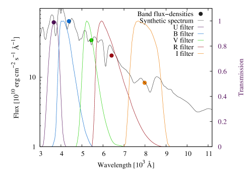
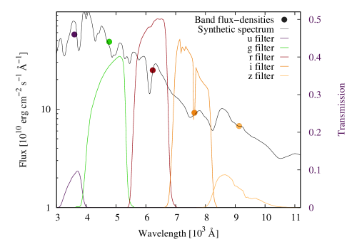
Figure 7: Left panel: The Hsiao template spectrum at maximum light and the transmission curves of the Johnson-Cousins $UBVRI$ system. Filled symbols indicate the synthetic flux densities. Right panel: the same but for the Sloan $u^{\prime}g^{\prime}r^{\prime}i^{\prime}z^{\prime}$ system.

Since MLCS2k2 is originally designed for only the $UBVRI$ system (Jha, Riess & Kirshner, 2007), one needs to transform its $M_{X}$, $P_{X}$ and $Q_{X}$ vectors ($X=\{U,B,V,R,I\}$) to other filters if data from other photometric system are to be fit. We have computed the transformation to the Sloan $u^{\prime}g^{\prime}r^{\prime}i^{\prime}z^{\prime}$ system via the Hsiao template spectra (Hsiao et al., 2007) in the following way.

First, synthetic fluxes for both $UBVRI$ and $u^{\prime}g^{\prime}r^{\prime}i^{\prime}z^{\prime}$ filters were computed from the Hsiao template spectra by convolving the templates with the corresponding filter functions (Fig.7). This was done for all templates between $-10$ day and $+90$ day. Next, the following flux ratios were defined as the basis of the $UBVRI$ $\rightarrow$ $u^{\prime}g^{\prime}r^{\prime}i^{\prime}z^{\prime}$ transformation: $f(u^{\prime})/f(U)$, $f(g^{\prime})/f(B)$, $f(r^{\prime})/f(R)$, $f(i^{\prime})/f(I)$ and $f(z^{\prime})/f(I)$. Among many other combinations, these flux ratios were found to exhibit the least amount of variation in the $[-10$d,+90d$]$ phase interval. Third, using these flux ratios the MLCS2k2 $UBVRI$ magnitudes were transformed to fluxes, multiplied by the corresponding flux ratios and converted back to Sloan $u^{\prime}g^{\prime}r^{\prime}i^{\prime}z^{\prime}$ magnitudes. Note that this conversion is based on the implicit assumption that the above flux ratios remain the same for SNe having different MLCS2k2 $\Delta$ parameter. This certainly breaks down for SNe having large ($>0.5$) $\Delta$; however, since our SNe have only $\Delta$ within $\pm 0.3$, this assumption should be approximately valid. The feasibility of the whole transformation can also be judged by the consistency between the MLCS2k2 fitting parameters computed from the quasi-simultaneous $UBVRI$ and $u^{\prime}g^{\prime}r^{\prime}i^{\prime}z^{\prime}$ data.

MLCS2k2 also contains a prescription for the time-dependence of the extinction in the $UBVRI$ bands, parametrized as $\zeta_{X}(t)=A_{X}(t)/A_{X}(t_{Bmax})$, where $A_{X}$ is the extinction in the $X$-band. We transformed the $\zeta_{X}$ vectors of Jha, Riess & Kirshner (2007) to the $u^{\prime}g^{\prime}r^{\prime}i^{\prime}z^{\prime}$ system using a similar approach as above. First, following Jha, Riess & Kirshner (2007), the Hsiao templates were reddened with a chosen $A_{V}$ and using the Cardelli-law (Cardelli et al., 1989):

$${A(x)\over A_{V}}=({\alpha}(x)+{{\beta}(x)\over R_{V}}).$$ (A1)

The standard Milky Way reddening slope, $R_{V}=3.1$, was assumed at first, but this condition was relaxed later (see below).

Next, both the reddened and the reddening-free $UBVRI$ magnitudes were transformed to $u^{\prime}g^{\prime}r^{\prime}i^{\prime}z^{\prime}$ magnitudes as above, and their time-dependent differences were used to construct the $\zeta$ vectors for the Sloan system: $\zeta_{X}=(M^{\prime}_{X}(t)-M_{X}(t))/(M^{\prime}_{X}(t_{Bmax})-M_{X}(t_{Bmax}))$, where $M^{\prime}_{X}$ denotes the reddened MLCS2k2 magnitude in the $X$-band.

To be able to handle non-standard (i.e. $R_{V}\neq 3.1$) reddening slopes, the procedure described above has been repeated for $1<R_{V}<6$. It was found that the resulting $\zeta_{X}(R_{V})$ values as a function of $1-\zeta_{X}(3.1)$ can be approximated by a parabola of the following form:

$$1-\zeta_{X}(R_{V})=a_{X}\cdot(1-\zeta_{X}(3.1))^{2}+b_{X}\cdot(1-\zeta_{X}(3.1))+c_{X}.$$ (A2)

Since the $a_{X}$, $b_{X}$ and $c_{X}$ coefficients are different for every $R_{V}$, their dependency on $R_{V}$ were determined by fitting a cubic polynomial to these data as a function of $R_{V}^{-1}$:

$$a_{X} = d_{1,1}\cdot(R_{V}^{-1})^{3}+d_{1,2}\cdot(R_{V}^{-1})^{2}+d_{1,3}\cdot(R_{V}^{-1})+d_{1,4}$$

$$b_{X} = d_{2,1}\cdot(R_{V}^{-1})^{3}+d_{2,2}\cdot(R_{V}^{-1})^{2}+d_{2,3}\cdot(R_{V}^{-1})+d_{2,4}$$ (A3)

$$c_{X} = d_{3,1}\cdot(R_{V}^{-1})^{3}+d_{3,2}\cdot(R_{V}^{-1})^{2}+d_{3,3}\cdot(R_{V}^{-1})+d_{3,4}$$

The fit parameters for both photometric systems are collected in Table 10.

Table 10: The constant parameters from the third-order polynomial fit to $a_{X}$, $b_{X}$ and $c_{X}$ as functions of $R_{V}^{-1}$ (see Eq.A).

	$U$	$B$	$V$	$R$	$I$	$u^{\prime}$	$g^{\prime}$	$r^{\prime}$	$i^{\prime}$	$z^{\prime}$
$d_{1,1}$	-29.637	1.711	0.355	-1.157	-11.212	-41.028	4.925	-0.974	-8.647	-193.074
$d_{2,1}$	2.790	0.845	0.023	0.235	5.962	2.828	0.424	0.120	-1.468	13.272
$d_{3,1}\cdot 10^{-3}$	0.149	-0.222	0.053	0.157	-6.828	-0.126	1.938	0.028	-0.718	44.466
$d_{1,2}$	81.694	-5.761	-0.618	-1.431	9.372	108.431	-9.990	-0.590	0.074	218.568
$d_{2,2}$	-7.388	-2.551	-0.236	0.339	-4.992	-5.476	-1.879	0.268	6.286	-15.035
$d_{3,2}\cdot 10^{-3}$	-0.443	0.777	-0.676	0.215	5.714	-1.256	-3.057	0.051	-0.621	-50.453
$d_{1,3}$	-77.845	-0.101	-2.496	-3.137	-6.392	-79.613	5.363	6.273	1.242	-91.518
$d_{2,3}$	7.736	4.200	2.503	1.409	3.171	6.257	3.709	1.259	-2.521	6.292
$d_{3,3}\cdot 10^{-3}$	0.401	0.409	1.466	1.314	-3.743	0.560	0.973	0.785	0.378	21.295
$d_{1,4}$	17.612	0.573	0.855	1.199	1.443	15.798	-0.897	-1.937	-0.173	12.752
$d_{2,4}$	-0.822	-0.118	0.216	0.502	0.306	-0.545	-0.013	0.562	1.256	0.124
$d_{3,4}\cdot 10^{-3}$	-0.088	-0.205	-0.404	-0.452	0.831	-0.046	-0.084	-0.259	-0.043	-2.997

Appendix B Photometric data

Table 11: Local $BVRI$ standard stars in the vicinity of SN 2012cg

R.A.	Dec.	B	$\sigma_{B}$	V	$\sigma_{V}$	R	$\sigma_{R}$	I	$\sigma_{I}$
12:27:28.9	9:29:33.6	16.241	0.011	15.648	0.013	15.345	0.011	14.932	0.017
12:26:48.0	9:28:50.5	15.408	0.011	14.644	0.013	14.245	0.011	13.771	0.017
12:26:48.3	9:29:57.3	15.805	0.011	14.998	0.013	14.570	0.011	14.050	0.017
12:27:15.9	9:27:27.0	15.046	0.011	14.506	0.013	14.232	0.011	13.841	0.017
12:27:29.8	9:23:53.2	15.919	0.011	15.078	0.013	14.633	0.011	14.106	0.017

Table 12: Photometry of SN 2012cg. The $BVRI$ data are given in Vega-magnitudes. Errors are given in parentheses.

MJD	B	V	R	I
56066.8	14.995 (0.031)	14.679 (0.025)	14.593 (0.023)	14.420 (0.048)
56067.9	14.493 (0.014)	14.221 (0.010)	14.133 (0.011)	13.974 (0.018)
56069.8	13.629 (0.014)	13.490 (0.010)	13.375 (0.009)	13.229 (0.018)
56072.9	12.765 (0.008)	12.674 (0.010)	12.575 (0.008)	12.462 (0.017)
56073.8	12.646 (0.015)	12.475 (0.016)	12.481 (0.012)	12.360 (0.019)
56075.8	12.452 (0.012)	12.175 (0.012)	12.233 (0.007)	12.179 (0.017)
56076.8	12.141 (0.017)	12.172 (0.011)	12.108 (0.011)	12.110 (0.022)
56077.8	12.205 (0.011)	12.150 (0.009)	12.105 (0.009)	12.061 (0.017)
56079.9	12.132 (0.008)	12.018 (0.010)	11.994 (0.008)	12.032 (0.015)
56080.8	12.150 (0.013)	11.995 (0.012)	11.954 (0.009)	12.058 (0.018)
56081.8	12.097 (0.017)	11.951 (0.015)	11.950 (0.012)	12.055 (0.022)
56084.9	12.139 (0.010)	11.904 (0.013)	11.888 (0.012)	12.097 (0.023)
56089.9	12.439 (0.016)	12.055 (0.023)	12.042 (0.024)	12.352 (0.030)
56092.9	12.617 (0.018)	12.258 (0.010)	12.296 (0.008)	12.540 (0.019)
56093.9	12.726 (0.018)	12.325 (0.021)	12.354 (0.012)	12.606 (0.032)
56094.9	12.799 (0.025)	12.355 (0.020)	12.441 (0.013)	12.635 (0.034)
56095.9	12.918 (0.033)	12.462 (0.021)	12.502 (0.014)	12.659 (0.031)
56097.9	13.143 (0.032)	12.576 (0.022)	12.550 (0.018)	12.659 (0.032)
56098.9	13.251 (0.027)	12.629 (0.022)	12.611 (0.010)	12.647 (0.028)
56099.9	13.389 (0.025)	12.677 (0.021)	12.644 (0.017)	12.630 (0.031)
56101.9	13.565 (0.025)	12.834 (0.020)	12.666 (0.010)	12.607 (0.027)
56102.9	13.756 (0.029)	12.884 (0.023)	12.640 (0.018)	12.571 (0.031)
56104.9	13.992 (0.032)	12.951 (0.026)	12.728 (0.013)	12.568 (0.032)

Table 13: Local $BVRI$ standard stars in the vicinity of SN 2012ht

R.A.	Dec.	B	$\sigma_{B}$	V	$\sigma_{V}$	R	$\sigma_{R}$	I	$\sigma_{I}$
10:53:01.648	+16:56:03.06	14.886	0.009	14.225	0.011	13.787	0.014	13.405	0.007
10:54:06.561	+16:45:53.13	15.589	0.005	14.944	0.006	14.697	0.005	14.505	0.009
10:53:39.512	+16:49:17.04	15.914	0.005	15.300	0.006	14.991	0.005	14.575	0.006
10:54:01.309	+16:50:07.90	15.759	0.005	15.149	0.006	14.841	0.005	14.426	0.006
10:52:54.642	+16:59:01.96	15.253	0.010	14.524	0.013	13.995	0.016	13.555	0.008
10:53:05.252	+16:50:56.91	15.838	0.005	15.149	0.006	14.799	0.005	14.354	0.006
10:54:01.439	+16:51:57.31	16.054	0.005	15.160	0.006	14.686	0.005	14.107	0.005
10:52:57.121	+16:54:56.27	15.751	0.006	14.975	0.007	14.497	0.007	13.958	0.007

Table 14: Photometry of SN 2012ht. The $BVRI$ data are given in Vega-magnitudes, while the $g^{\prime}r^{\prime}i^{\prime}z^{\prime}$ data are in AB-magnitudes.

MJD	B	$\sigma_{B}$	V	$\sigma_{V}$	R	$\sigma_{R}$	I	$\sigma_{I}$
56066.8	14.995	0.031	14.679	0.025	14.593	0.023	14.420	0.048
56067.9	14.493	0.014	14.221	0.010	14.133	0.011	13.974	0.018
56069.8	13.629	0.014	13.490	0.010	13.375	0.009	13.229	0.018
56072.9	12.765	0.008	12.674	0.010	12.575	0.008	12.462	0.017
56073.8	12.646	0.015	12.475	0.016	12.481	0.012	12.360	0.019
56075.8	12.452	0.012	12.175	0.012	12.233	0.007	12.179	0.017
56076.8	12.141	0.017	12.172	0.011	12.108	0.011	12.110	0.022
56077.8	12.205	0.011	12.150	0.009	12.105	0.009	12.061	0.017
56079.9	12.132	0.008	12.018	0.010	11.994	0.008	12.032	0.015
56080.8	12.150	0.013	11.995	0.012	11.954	0.009	12.058	0.018
56081.8	12.097	0.017	11.951	0.015	11.950	0.012	12.055	0.022
56084.9	12.139	0.010	11.904	0.013	11.888	0.012	12.097	0.023
56089.9	12.439	0.016	12.055	0.023	12.042	0.024	12.352	0.030
56092.9	12.617	0.018	12.258	0.010	12.296	0.008	12.540	0.019
56093.9	12.726	0.018	12.325	0.021	12.354	0.012	12.606	0.032
56094.9	12.799	0.025	12.355	0.020	12.441	0.013	12.635	0.034
56095.9	12.918	0.033	12.462	0.021	12.502	0.014	12.659	0.031
56097.9	13.143	0.032	12.576	0.022	12.550	0.018	12.659	0.032
56098.9	13.251	0.027	12.629	0.022	12.611	0.010	12.647	0.028
56099.9	13.389	0.025	12.677	0.021	12.644	0.017	12.630	0.031
56101.9	13.565	0.025	12.834	0.020	12.666	0.010	12.607	0.027
56102.9	13.756	0.029	12.884	0.023	12.640	0.018	12.571	0.031
56104.9	13.992	0.032	12.951	0.026	12.728	0.013	12.568	0.032
MJD	g	$\sigma_{g}$	r	$\sigma_{r}$	i	$\sigma_{i}$	z	$\sigma_{z}$
56285.94	14.182	0.227	14.074	0.094	14.277	0.087	–	–
56290.01	13.508	0.107	13.444	0.039	13.657	0.062	13.867	0.075
56291.14	13.347	0.151	13.375	0.094	13.673	0.073	13.730	0.107
56292.11	13.383	0.147	13.250	0.115	13.513	0.119	13.883	0.126
56303.97	13.402	0.140	13.518	0.119	14.306	0.167	14.335	0.173
56315.94	14.700	0.270	14.037	0.109	14.457	0.215	14.213	0.410
56322.94	15.277	0.288	14.537	0.098	14.658	0.188	14.368	0.189
56326.86	15.458	0.202	14.757	0.064	14.873	0.189	14.551	0.178
56330.97	15.601	0.129	14.964	0.078	15.180	0.110	14.953	0.211
56331.91	15.529	0.047	15.003	0.113	15.195	0.121	14.988	0.170
56340.92	15.975	0.153	15.477	0.100	15.616	0.138	15.482	0.157
56351.86	16.162	0.226	15.896	0.143	15.649	0.224	15.316	0.293
56353.86	16.122	0.122	15.815	0.135	16.081	0.188	16.085	0.156
56355.96	16.199	0.199	15.931	0.146	16.201	0.203	16.393	0.254
56356.80	16.392	0.181	15.958	0.181	16.205	0.191	16.624	0.289
56362.91	16.372	0.208	16.206	0.149	16.424	0.224	16.468	0.236
56388.80	16.875	0.175	17.059	0.151	17.456	0.232	17.738	0.394
56395.91	17.092	0.166	17.087	0.045	17.444	0.143	18.357	0.488
56396.80	16.949	0.146	17.281	0.152	17.330	0.241	18.708	1.002
56397.80	16.947	0.133	17.180	0.060	17.666	0.157	18.496	0.410
56398.86	16.930	0.093	17.348	0.100	17.499	0.104	17.457	0.191

Table 15: Local $BVRI$ standard stars in the vicinity of SN 2013dy

R.A.	Dec.	B	$\sigma_{B}$	V	$\sigma_{V}$	R	$\sigma_{R}$	I	$\sigma_{I}$
22:18:22.19	+40:34:21.9	16.233	0.032	15.606	0.014	15.243	0.015	14.844	0.016
22:18:16.96	+40:34:55.9	15.539	0.033	14.927	0.011	14.584	0.015	14.216	0.016

Table 16: $BVRI$ photometry of SN 2013dy, given in the Vega-system

MJD	B	$\sigma_{B}$	V	$\sigma_{V}$	R	$\sigma_{R}$	I	$\sigma_{I}$
56490.9	14.069	0.008	13.824	0.033	13.653	0.045	13.522	0.031
56492.0	13.929	0.021	13.636	0.032	13.459	0.064	13.341	0.065
56493.0	13.720	0.093	13.479	0.022	13.307	0.062	13.205	0.040
56494.0	13.584	0.067	13.359	0.011	13.196	0.070	13.103	0.038
56494.9	13.492	0.028	13.271	0.002	13.118	0.059	13.042	0.039
56495.9	13.388	0.064	13.168	0.038	13.050	0.067	12.980	0.055
56496.9	13.376	0.052	13.118	0.041	12.998	0.088	12.955	0.038
56497.9	13.325	0.045	13.036	0.066	12.954	0.057	12.950	0.030
56498.8	13.282	0.027	13.028	0.022	12.934	0.051	12.957	0.042
56499.8	13.274	0.076	13.043	0.002	12.902	0.063	12.970	0.058
56500.8	13.316	0.002	12.981	0.021	12.913	0.068	12.983	0.043
56501.8	13.255	0.002	12.957	0.034	12.874	0.063	13.010	0.048
56505.8	13.415	0.010	13.006	0.040	12.939	0.059	13.135	0.055
56506.9	13.427	0.030	13.044	0.030	12.960	0.065	13.203	0.026
56507.9	13.489	0.044	13.070	0.048	13.004	0.075	13.250	0.049
56509.8	13.610	0.064	13.153	0.019	13.112	0.061	13.369	0.059
56511.8	13.748	0.074	13.268	0.029	13.248	0.069	13.499	0.060
56512.8	13.827	0.068	13.335	0.033	13.332	0.054	13.569	0.034
56520.9	14.717	0.060	13.801	0.012	13.622	0.051	13.614	0.045
56521.9	14.819	0.039	13.849	0.058	13.652	0.055	13.588	0.054
56534.8	15.934	0.001	14.382	0.045	13.972	0.064	13.528	0.030
56536.8	16.040	0.013	14.518	0.031	14.089	0.043	13.619	0.048
56538.8	16.127	0.040	14.624	0.016	14.198	0.073	13.750	0.028
56539.8	16.166	0.043	14.677	0.007	14.265	0.053	13.808	0.027
56541.8	16.215	0.024	14.782	0.044	14.389	0.065	13.928	0.053
56542.8	16.271	0.047	14.843	0.018	14.433	0.068	13.998	0.046
56554.9	16.465	0.038	15.236	0.017	14.898	0.052	14.621	0.059
56563.0	16.568	0.022	15.473	0.036	15.167	0.046	14.980	0.044
56566.8	16.598	0.035	15.559	0.025	15.288	0.062	15.160	0.035
56573.8	16.701	0.054	15.760	0.023	15.513	0.053	15.424	0.043
56577.8	16.730	0.042	15.866	0.027	15.625	0.059	15.588	0.014
56590.9	16.905	0.061	16.182	0.028	16.021	0.067	16.073	0.046
56591.9	16.912	0.018	16.203	0.043	16.052	0.050	16.099	0.027
56596.7	16.973	0.042	16.328	0.012	16.200	0.035	16.294	0.030
56603.9	17.017	0.054	16.584	0.026	16.424	0.064	16.540	0.066

Table 17: $g^{\prime}r^{\prime}i^{\prime}z^{\prime}$ photometry of SN 2013dy, given as AB-magnitudes

MJD	g	$\sigma_{g}$	r	$\sigma_{r}$	i	$\sigma_{i}$	z	$\sigma_{z}$
56490.92	13.901	0.079	13.689	0.060	13.789	0.050	13.901	0.131
56491.90	13.705	0.110	13.481	0.057	13.557	0.078	13.607	0.121
56492.91	13.623	0.101	13.332	0.068	13.365	0.086	13.527	0.115
56493.91	13.534	0.124	13.198	0.041	13.320	0.047	13.463	0.074
56494.91	13.462	0.115	13.174	0.051	13.313	0.063	13.440	0.083
56495.88	13.377	0.130	13.100	0.056	13.271	0.068	13.364	0.079
56496.84	13.176	0.103	13.036	0.094	13.257	0.092	13.473	0.203
56497.85	13.349	0.134	13.022	0.050	13.272	0.065	13.336	0.121
56498.89	13.170	0.104	12.924	0.079	13.201	0.074	13.237	0.080
56502.90	13.036	0.061	12.980	0.063	13.237	0.119	13.335	0.138
56503.93	13.017	0.070	12.888	0.032	13.366	0.045	13.322	0.108
56504.88	13.120	0.082	12.882	0.036	13.373	0.059	13.330	0.099
56505.88	12.998	0.058	12.895	0.041	13.449	0.044	13.334	0.088
56508.88	13.160	0.068	13.005	0.038	13.558	0.079	13.605	0.108
56509.84	13.217	0.071	13.112	0.048	13.587	0.077	13.579	0.116
56510.86	13.209	0.048	13.175	0.033	13.726	0.041	13.600	0.155
56511.84	13.426	0.083	13.222	0.053	13.745	0.064	13.656	0.134
56512.85	13.394	0.064	13.315	0.031	13.872	0.054	13.842	0.136
56513.85	13.622	0.085	13.416	0.051	13.938	0.102	13.670	0.085
56515.86	13.520	0.050	13.496	0.032	14.060	0.050	13.651	0.083
56519.83	14.033	0.108	13.608	0.045	14.033	0.074	13.647	0.096
56520.83	14.096	0.097	13.617	0.053	14.086	0.065	13.736	0.143
56521.82	14.133	0.091	13.660	0.055	14.036	0.064	13.644	0.124
56526.82	14.525	0.159	13.803	0.088	13.916	0.097	13.582	0.087
56530.87	14.663	0.067	13.826	0.054	13.913	0.053	13.580	0.125
56534.87	14.812	0.061	13.959	0.029	13.977	0.035	13.640	0.100
56535.79	14.929	0.077	14.060	0.046	14.121	0.096	13.792	0.215
56538.82	15.068	0.053	14.214	0.044	14.200	0.061	13.836	0.112
56539.81	15.108	0.067	14.252	0.033	14.261	0.043	13.921	0.126
56541.79	15.152	0.051	14.348	0.035	14.371	0.059	13.991	0.126
56542.83	15.225	0.057	14.380	0.031	14.412	0.064	14.071	0.126
56543.83	15.377	0.118	14.487	0.051	14.463	0.067	14.187	0.098
56551.76	15.989	0.190	14.911	0.082	15.037	0.113	14.768	0.153
56552.80	15.496	0.103	14.731	0.054	14.866	0.077	14.616	0.123
56554.83	15.782	0.162	14.813	0.043	14.900	0.052	14.880	0.101
56557.79	15.536	0.100	14.899	0.062	14.908	0.075	14.920	0.150
56558.90	15.572	0.085	14.879	0.036	15.002	0.053	14.842	0.099
56559.77	15.496	0.066	14.939	0.033	15.049	0.046	15.022	0.142
56560.76	15.517	0.078	14.978	0.052	15.071	0.068	15.149	0.207
56568.79	15.570	0.068	15.117	0.042	15.269	0.063	15.257	0.082
56569.77	15.636	0.066	15.188	0.058	15.240	0.064	15.241	0.135
56575.91	15.752	0.074	15.262	0.049	15.444	0.067	15.529	0.129
56578.73	15.815	0.095	15.325	0.046	15.479	0.055	15.537	0.116
56582.90	16.002	0.110	15.504	0.062	15.520	0.068	15.640	0.119
56584.74	15.941	0.132	15.432	0.055	15.952	0.131	15.511	0.131
56586.78	15.976	0.102	15.548	0.058	15.726	0.074	15.618	0.108
56588.81	15.836	0.091	15.538	0.058	15.659	0.060	15.863	0.136
56590.80	15.880	0.081	15.650	0.069	15.705	0.061	15.781	0.139
56591.77	15.842	0.061	15.533	0.038	15.645	0.059	15.759	0.109
56594.73	15.907	0.048	15.652	0.050	15.743	0.063	16.255	0.201
56595.98	16.008	0.092	15.909	0.129	15.789	0.102	16.586	0.356
56597.97	15.893	0.134	15.911	0.126	15.958	0.182	16.909	0.590
56603.75	15.991	0.052	15.709	0.037	15.882	0.052	15.871	0.103
56627.82	16.224	0.072	16.012	0.058	16.025	0.076	16.152	0.180
56628.82	16.319	0.085	16.127	0.089	16.120	0.084	15.890	0.149

Table 18: Local $BVRI$ standard stars in the vicinity of SN 2014J

R.A.	Dec.	B	$\sigma_{B}$	V	$\sigma_{V}$	R	$\sigma_{R}$	I	$\sigma_{I}$
09:56:37.96	+69:41:18.9	15.024	0.012	14.277	0.010	13.855	0.007	13.396	0.010
09:56:32.99	+69:39:17.9	13.983	0.008	13.504	0.007	13.209	0.005	12.816	0.008

Table 19: Photometry of SN 2014J. The $BVRI$ data are given in Vega-magnitudes, while the $g^{\prime}r^{\prime}i^{\prime}z^{\prime}$ data are in AB-magnitudes.

MJD	B	$\sigma_{B}$	V	$\sigma_{V}$	R	$\sigma_{R}$	I	$\sigma_{I}$
56684.0	12.142	0.040	10.921	0.018	10.282	0.003	9.802	0.031
56688.8	11.846	0.068	10.669	0.015	10.093	0.028	9.697	0.002
56691.0	11.971	0.117	10.622	0.025	10.040	0.008	9.827	0.004
56692.0	11.931	0.081	10.588	0.037	10.071	0.015	9.858	0.020
56693.0	11.965	0.032	10.584	0.031	10.078	0.027	9.819	0.011
56703.0	12.818	0.020	11.136	0.022	10.655	0.013	10.367	0.005
56706.2	13.211	0.071	11.345	0.041	10.835	0.018	10.348	0.027
56709,0	13.538	0.085	11.362	0.071	10.770	0.037	10.280	0.078
56712.0	13.745	0.020	11.458	0.027	10.789	0.007	10.122	0.004
56717.8	14.521	0.001	11.726	0.002	10.995	0.004	10.184	0.012
56724.9	14.822	0.024	12.179	0.021	11.326	0.009	10.425	0.010
56726.0	14.944	0.035	12.152	0.026	11.371	0.014	10.480	0.015
56727.0	15.009	0.040	12.250	0.008	11.457	0.003	10.545	0.019
56728.0	14.969	0.006	12.343	0.040	11.537	0.018	10.632	0.020
56729.0	15.060	0.006	12.367	0.041	11.550	0.001	10.687	0.030
56730.9	15.003	0.002	12.438	0.019	11.650	0.023	10.643	0.008
56736.9	15.042	0.004	12.659	0.006	11.904	0.005	11.148	0.015
56739.0	15.124	0.017	12.714	0.016	11.958	0.043	11.034	0.024
56741.9	15.169	0.018	12.792	0.019	12.035	0.002	11.238	0.005
56742.8	15.156	0.001	12.809	0.001	12.065	0.001	11.371	0.001
56744.8	15.142	0.026	12.855	0.002	11.920	0.014	11.370	0.012
56746.0	15.198	0.017	12.916	0.022	12.092	0.005	11.411	0.011
56746.9	15.200	0.001	12.938	0.007	12.060	0.007	11.480	0.009
56751.8	15.223	0.019	13.045	0.018	12.318	0.008	11.711	0.025
56754.8	15.248	0.030	13.124	0.008	12.420	0.007	11.790	0.006
56774.8	15.215	0.029	13.602	0.004	12.945	0.007	12.480	0.013
56777.9	15.407	0.008	13.682	0.021	13.062	0.004	12.608	0.035
56785.8	15.405	0.043	13.829	0.002	13.199	0.010	12.731	0.008
56798.9	15.571	0.014	14.108	0.020	13.545	0.007	13.078	0.025
MJD	g	$\sigma_{g}$	r	$\sigma_{r}$	i	$\sigma_{i}$	z	$\sigma_{z}$
56680.05	12.295	0.030	10.941	0.056	10.836	0.023	10.415	0.034
56682.97	11.733	0.033	10.554	0.063	10.397	0.013	10.072	0.037
56683.97	11.582	0.018	10.504	0.081	10.281	0.033	9.872	0.058
56691.07	11.267	0.014	10.213	0.012	10.311	0.019	9.977	0.029
56692.10	11.278	0.016	10.199	0.007	10.340	0.016	10.018	0.032
56692.97	11.284	0.011	10.218	0.012	10.354	0.016	10.044	0.038
56698.12	11.414	0.016	10.435	0.004	10.610	0.026	10.172	0.024
56700.98	11.540	0.017	10.694	0.020	10.967	0.046	10.269	0.033
56701.79	11.627	0.010	10.719	0.010	10.908	0.031	10.254	0.033
56702.97	11.687	0.012	10.787	0.011	10.970	0.028	10.267	0.039
56703.76	11.718	0.005	10.851	0.006	10.970	0.023	10.259	0.052
56713.90	12.509	0.017	10.958	0.010	10.821	0.032	10.075	0.037
56714.84	12.518	0.015	10.990	0.014	10.749	0.021	10.104	0.034
56715.77	12.572	0.029	10.987	0.017	10.734	0.019	10.091	0.062
56717.85	12.697	0.012	11.069	0.011	10.815	0.030	10.124	0.038
56719.91	12.879	0.011	11.134	0.010	10.878	0.023	10.116	0.030
56724.97	13.230	0.009	11.489	0.012	11.133	0.026	10.336	0.035
56725.86	13.225	0.021	11.581	0.010	11.182	0.026	10.443	0.035
56727.93	13.375	0.014	11.650	0.016	11.336	0.030	10.509	0.036
56728.93	13.467	0.020	11.747	0.012	11.424	0.029	10.584	0.034
56729.95	13.473	0.027	11.765	0.016	11.489	0.035	10.620	0.030
56730.80	13.400	0.022	11.807	0.012	11.471	0.030	10.752	0.034
56733.93	13.552	0.016	11.961	0.017	11.614	0.032	10.938	0.029
56734.75	13.457	0.047	11.899	0.057	11.565	0.035	11.144	0.053
56737.85	13.627	0.013	12.047	0.018	11.760	0.033	11.074	0.040
56745.79	13.815	0.011	12.297	0.019	12.063	0.039	11.482	0.040
56746.92	13.748	0.104	12.300	0.035	12.112	0.051	11.655	0.119
56754.82	13.980	0.016	12.558	0.022	12.293	0.040	11.866	0.049
56768.80	14.227	0.020	12.910	0.030	12.682	0.047	12.493	0.052
56769.88	14.236	0.018	12.965	0.029	12.715	0.044	12.390	0.058
56773.86	14.314	0.018	13.079	0.028	12.852	0.046	12.551	0.058
56775.88	14.255	0.028	13.095	0.034	12.896	0.054	12.976	0.114
56782.84	14.382	0.024	13.294	0.029	13.037	0.052	12.750	0.058
56783.84	14.464	0.018	13.346	0.028	13.060	0.056	12.849	0.069
56785.81	14.512	0.019	13.361	0.032	13.098	0.052	12.828	0.062
56787.86	14.547	0.022	13.384	0.032	13.114	0.055	12.887	0.069
56796.91	14.654	0.029	13.628	0.049	13.388	0.068	13.056	0.081
56797.88	14.672	0.025	13.604	0.049	13.312	0.068	13.033	0.085
56798.84	14.670	0.029	13.603	0.043	13.245	0.057	12.918	0.068
56799.89	14.686	0.022	13.633	0.037	13.305	0.060	13.097	0.076
56805.87	14.834	0.028	13.747	0.054	13.362	0.077	13.156	0.084
56811.86	14.898	0.035	13.893	0.052	13.530	0.072	13.187	0.088

References

- Amanullah et al. (2014) Amanullah, R., Goobar, A., Johansson, J., et al. 2014, ApJ, 788, L21
- Amanullah et al. (2015) Amanullah, R., Johansson, J., Goobar, A., et al. 2015, MNRAS, 453, 3300
- Astier et al. (2006) Astier, P., Guy, J., Regnault, N., et al. 2006, A&A, 447, 31
- Benitez-Herrera et al. (2013) Benitez-Herrera, S., Ishida, E. E. O., Maturi, M., et al. 2013, MNRAS, 436, 854
- Betoule et al. (2014) Betoule, M., Kessler, R., Guy, J., et al. 2014, A&A, 568, A22
- Brown et al. (2015) Brown, P. J., Smitka, M. T., Wang, L., et al. 2015, ApJ, 805, 74
- Burns et al. (2011) Burns, C. R., Stritzinger, M., Phillips, M. M., et al. 2011, AJ, 141, 19
- Burns et al. (2014) Burns, C. R., Stritzinger, M., Phillips, M. M., et al. 2014, ApJ, 789, 32
- Cardelli et al. (1989) Cardelli, J. A., Clayton, G. C., & Mathis, J. S. 1989, ApJ, 345, 245
- Conley et al. (2008) Conley, A., Sullivan, M., Hsiao, E. Y., et al. 2008, ApJ, 681, 482-498
- Conley et al. (2011) Conley, A., Guy, J., Sullivan, M., et al. 2011, ApJS, 192, 1
- Cortés et al. (2006) Cortés, J. R., Kenney, J. D. P., & Hardy, E. 2006, AJ, 131, 747
- Dale et al. (2007) Dale, D. A., Gil de Paz, A., Gordon, K. D., et al. 2007, ApJ, 655, 863
- Dhawan et al. (2017) Dhawan, S., Jha, S. W., & Leibundgut, B. 2017, arXiv:1707.00715
- Draine (2003) Draine, B. T. 2003, ARA&A, 41, 241
- Folatelli et al. (2010) Folatelli, G., Phillips, M. M., Burns, C. R., et al. 2010, AJ, 139, 120
- Foley et al. (2014) Foley, R. J., Fox, O. D., McCully, C., et al. 2014, MNRAS, 443, 2887
- Fossey et al. (2014) Fossey, S. J., Cooke, B., Pollack, G., Wilde, M., & Wright, T. 2014, Central Bureau Electronic Telegrams, 3792, 1
- Friedman et al. (2015) Friedman, A. S., Wood-Vasey, W. M., Marion, G. H., et al. 2015, ApJS, 220, 9
- Gao et al. (2015) Gao, J., Jiang, B. W., Li, A., Li, J., & Wang, X. 2015, ApJ, 807, L26
- Goobar et al. (2014) Goobar, A., Johansson, J., Amanullah, R., et al. 2014, ApJ, 784, L12
- Guy et al. (2007) Guy, J., Astier, P., Baumont, S., et al. 2007, A&A, 466, 11
- Guy et al. (2010) Guy, J., Sullivan, M., Conley, A., et al. 2010, A&A, 523, A7
- Hicken et al. (2009) Hicken, M., Wood-Vasey, W. M., Blondin, S., et al. 2009, ApJ, 700, 1097
- Hsiao et al. (2007) Hsiao, E. Y., Conley, A., Howell, D. A., et al. 2007, ApJ, 663, 1187
- Jha et al. (1999) Jha, S., Garnavich, P. M., Kirshner, R. P., et al. 1999, ApJS, 125, 73
- Jha, Riess & Kirshner (2007) Jha, S., Riess, A. G., & Kirshner, R. P. 2007, ApJ, 659, 122
- Jordi et al. (2006) Jordi, K., Grebel, E. K., & Ammon, K. 2006, A&A, 460, 339
- Kelly et al. (2010) Kelly, P. L., Hicken, M., Burke, D. L., Mandel, K. S., & Kirshner, R. P. 2010, ApJ, 715, 743
- Kessler et al. (2009) Kessler, R., Becker, A. C., Cinabro, D., et al. 2009, ApJS, 185, 32
- Lampeitl et al. (2010) Lampeitl, H., Smith, M., Nichol, R. C., et al. 2010, ApJ, 722, 566
- Le Borgne & Rocca-Volmerange (2002) Le Borgne, D., & Rocca-Volmerange, B. 2002, A&A, 386, 446
- Mandel et al. (2011) Mandel, K. S., Narayan, G., & Kirshner, R. P. 2011, ApJ, 731, 120
- Marion et al. (2015a) Marion, G. H., Sand, D. J., Hsiao, E. Y., et al. 2015, ApJ, 798, 39
- Marion et al. (2015b) Marion, G. H., Brown, P. J., Vinkó, J., et al. 2015, arXiv:1507.07261
- Mazzei et al. (2017) Mazzei, P., Marino, A., Rampazzo, R., et al. 2017, arXiv:1710.07474
- Mosher et al. (2014) Mosher, J., Guy, J., Kessler, R., et al. 2014, ApJ, 793, 16
- Munari et al. (2013) Munari, U., Henden, A., Belligoli, R., et al. 2013, New A, 20, 30
- Pan et al. (2014) Pan, Y.-C., Sullivan, M., Maguire, K., et al. 2014, MNRAS, 438, 1391
- Pan et al. (2015) Pan, Y.-C., Foley, R. J., Kromer, M., et al. 2015, MNRAS, 452, 4307
- Pereira et al. (2013) Pereira, R., Thomas, R. C., Aldering, G., et al. 2013, A&A, 554, A27
- Perlmutter et al. (1999) Perlmutter, S., Aldering, G., Goldhaber, G., et al. 1999, ApJ, 517, 565
- Phillips (1993) Phillips, M. M. 1993, ApJ, 413, L105
- Planck Collaboration et al. (2014) Planck Collaboration, Ade, P. A. R., Aghanim, N., et al. 2014, A&A, 571, A16
- Planck Collaboration et al. (2015) Planck Collaboration, Ade, P. A. R., Aghanim, N., et al. 2015, arXiv:1502.01589
- Poznanski et al. (2012) Poznanski, D., Prochaska, J. X., & Bloom, J. S. 2012, MNRAS, 426, 1465
- Prieto et al. (2006) Prieto, J. L., Rest, A., & Suntzeff, N. B. 2006, ApJ, 647, 501
- Pskovskii (1977) Pskovskii, I. P. 1977, AZh, 54, 1188
- Rest et al. (2014) Rest, A., Scolnic, D., Foley, R. J., et al. 2014, ApJ, 795, 44
- Richmond et al. (1994) Richmond, M. W., Treffers, R. R., Filippenko, A. V., et al. 1994, AJ, 107, 1022
- Riess et al. (1998) Riess, A. G., Filippenko, A. V., Challis, P., et al. 1998, AJ, 116, 1009
- Riess et al. (2005) Riess, A. G., Li, W., Stetson, P. B., et al. 2005, ApJ, 627, 579
- Riess et al. (2007) Riess, A. G., Strolger, L.-G., Casertano, S., et al. 2007, ApJ, 659, 98
- Riess et al. (2011) Riess, A. G., Macri, L., Casertano, S., et al. 2011, ApJ, 730, 119
- Riess et al. (2016) Riess, A. G., Macri, L. M., Hoffmann, S. L., et al. 2016, ApJ, 826, 56
- Saunders et al. (2015) Saunders, C., Aldering, G., Antilogus, P., et al. 2015, ApJ, 800, 57
- Schlafly & Finkbeiner (2011) Schlafly, E. F., & Finkbeiner, D. P. 2011, ApJ, 737, 103
- Scolnic et al. (2014) Scolnic, D., Rest, A., Riess, A., et al. 2014, ApJ, 795, 45
- Scolnic et al. (2015) Scolnic, D., Casertano, S., Riess, A., et al. 2015, ApJ, 815, 117
- Scolnic & Kessler (2016) Scolnic, D., & Kessler, R. 2016, ApJ, 822, L35
- Shariff et al. (2016) Shariff, H., Dhawan, S., Jiao, X., et al. 2016, MNRAS, 463, 4311
- Silverman et al. (2012) Silverman, J. M., Ganeshalingam, M., Cenko, S. B., et al. 2012, ApJ, 756, L7
- Sullivan et al. (2010) Sullivan, M., Conley, A., Howell, D. A., et al. 2010, MNRAS, 406, 782
- Vinkó et al. (2012) Vinkó, J. et al. 2012, A&A546, 12
- Walker et al. (2015) Walker, E. S., Baltay, C., Campillay, A., et al. 2015, ApJS, 219, 13
- Weyant et al. (2017) Weyant, A., Wood-Vasey, W. M., Joyce, R., et al. 2017, arXiv:1703.02402
- Wood-Vasey et al. (2007) Wood-Vasey, W. M., Miknaitis, G., Stubbs, C. W., et al. 2007, ApJ, 666, 694
- Yamanaka et al. (2014) Yamanaka, M., Maeda, K., Kawabata, M., et al. 2014, ApJ, 782, L35
- Yusa et al. (2012) Yusa, T., Itagaki, K., Nakano, S., et al. 2012, Central Bureau Electronic Telegrams, 3349, 1
- Zhai et al. (2016) Zhai, Q., Zhang, J.-J., Wang, X.-F., et al. 2016, AJ, 151, 125
- Zhang et al. (2017) Zhang, B. R., Childress, M. J., Davis, T. M., et al. 2017, MNRAS, 471, 2254
- Zheng et al. (2013) Zheng, W., Silverman, J. M., Filippenko, A. V., et al. 2013, ApJ, 778, L15
- Zheng et al. (2014) Zheng, W., Shivvers, I., Filippenko, A. V., et al. 2014, ApJ, 783, L24