All-atom computations with irreversible Markov chains

Abstract

The event-chain Monte Carlo (ECMC) method is an irreversible Markov process based on the factorized Metropolis filter and the concept of lifted Markov chains. Here, ECMC is applied to all-atom models of multi-particle interactions that include the long-ranged Coulomb potential. We discuss a line-charge model for the Coulomb potential and demonstrate its equivalence with the standard Coulomb model with tin-foil boundary conditions. Efficient factorization schemes for the potentials used in all-atom water models are presented, before we discuss the best choice for lifting schemes for factors of more than three particles. The factorization and lifting schemes are then applied to simulations of point-charge and charged-dipole Coulomb gases, as well as to small systems of liquid water. For a locally charge-neutral system in three dimensions, the algorithmic complexity is $\mathcal{O}(N\log N)$ in the number $N$ of particles. In ECMC, a Particle–Particle method, it is achieved without the interpolating mesh required for the efficient implementation of other modern Coulomb algorithms. An event-driven, cell-veto-based implementation samples the equilibrium Boltzmann distribution using neither time-step approximations nor spatial cutoffs on the range of the interaction potentials. We discuss prospects and challenges for ECMC in soft condensed-matter and biological physics.

I Introduction

I.1 Irreversible Markov processes

Numerical methods are ubiquitous in the natural sciences, with Markov-chain Monte Carlo Metropolis et al. (1953) and molecular dynamics Alder and Wainwright (1957) playing central roles. Markov-chain Monte Carlo applies to any computational science problem that can be formulated as an (perhaps fictitious) equilibrium-statistical-physics system and whose solution requires sampling its probability distribution. As in physical and chemical systems, equilibrium within the computational context usually means that all probability flows vanish. This requirement is enforced by the detailed-balance condition, an essential ingredient of most Markov-chain Monte Carlo methods and notably of the Metropolis algorithm Krauth (2006). Monte Carlo algorithms usually take much time to approach equilibrium Levin, Peres, and Wilmer (2008), and, once in equilibrium, to generate independent samples. This is, in part, due to the fact that detailed balance leads to time-reversible Markov-chain dynamics, which is diffusive and therefore slow.

In recent years, a new class of irreversible “event-chain” Monte Carlo (ECMC) algorithms has been proposed Bernard, Krauth, and Wilson (2009); Michel, Kapfer, and Krauth (2014). ECMC algorithms violate detailed balance but satisfy a weaker global-balance condition. Configurations at large times sample the equilibrium distribution, but the asymptotic steady state comes with non-vanishing probability flows. In particle systems with periodic boundary conditions, for example, atoms may continue to move preferentially in certain directions. In continuous spin systems, likewise, configurations realize the equilibrium distribution even though spins rotate in a preferred way Nishikawa et al. (2015); Michel, Mayer, and Krauth (2015); Lei and Krauth (2018). ECMC moves (displacements of particles, rotations of spins, etc.) are infinitesimal and persistent: An “active” particle moves directly from one event to the next, that is, it continues to move until a proposed move is vetoed by a unique “target” particle, which in turn becomes the active particle. This passing of the active-particle label is called a lifting Diaconis, Holmes, and Neal (2000); Chen, Lovász, and Pak (1999) and this concept overcomes the characteristic rejections of randomly proposed finite moves in the Metropolis algorithm. ECMC algorithms are powerful Bernard and Krauth (2011); Michel, Kapfer, and Krauth (2014); Nishikawa et al. (2015); Lei and Krauth (2018): In a one-dimensional particle system, they were demonstrated to mix on shorter time scales than Markov chains that satisfy detailed balance Kapfer and Krauth (2017).

In ECMC, the traditional Metropolis acceptance criterion based on the change in potential is replaced by a consensus rule. This is the essence of the factorized Metropolis filter, which applies to translation-invariant systems with pair-wise interactions between particles Michel, Kapfer, and Krauth (2014) and, more generally, to models whose interactions can be split into sets of independent factors Harland et al. (2017). The ECMC algorithm does not compute the total system potential energy. This makes it very appealing for long-range-interacting systems, where this computation is costly. For Coulomb systems, ECMC altogether avoids traditional algorithms for the electrostatic potential de Leeuw, Perram, and Smith (1980), the dominant computational bottleneck for long-range-interacting models. Rather, the cell-veto algorithm Kapfer and Krauth (2016) efficiently establishes consensus on the acceptance or the rejection of a proposed move, even if all particles interact with each other. This is the starting point for the present work.

Generally, computations in statistical physics fall into two categories. They either aim at thermodynamic averages (energy, specific heat, spatial correlation functions, etc.) or at dynamic properties (time correlations, nucleation barriers, coarsening, etc.). In principle, the computation of thermodynamic averages is the realm of Markov-chain Monte Carlo, whereas the analysis of dynamical behavior calls on molecular dynamics, as it solves Newton’s equations of motion. Specifically, however, the field of large-scale all-atom computations with long-ranged interactions is today dominated by molecular dynamics for both categories. The dominance of molecular dynamics is rooted in two facts: Firstly, traditional Monte Carlo methods usually update just $\mathcal{O}(1)$ particles at a time, and the acceptation/rejection step then requires the exact computation of the change in potential. The best currently known algorithm Berthoumieux and Maggs (2010) for the change in potential after such a local update in a Coulomb system is of complexity $\mathcal{O}(\sqrt{N})$ so that one Monte Carlo sweep (a sequential update of all $N$ particles) requires $\mathcal{O}(N^{3/2})$ computations. In molecular dynamics, in contrast, the discretized Newton’s equations update all particle positions simultaneously, and the necessary computation of the forces on all particles comes at a cost of $\mathcal{O}(N\log N)$, much less than for a Monte Carlo sweep. Secondly, Newtonian dynamics conserves momentum and explores phase space more efficiently than the local Metropolis algorithm. This advantage of molecular dynamics over Monte Carlo is, for example, brought out by the different scaling of the velocity auto-correlation functions in the context of long-time tails Alder and Wainwright (1970); Wittmer et al. (2011).

The time evolution of molecular dynamics has physical meaning, but from an algorithmic point of view, it is constrained by the requirement that it must implement Newton’s law. As a result, there is no additional freedom to accelerate the exploration of phase space. In contrast, Monte Carlo dynamics is non-physical and only constrained by the global-balance condition. A well-chosen Monte Carlo dynamics can considerably speed up the sampling of the equilibrium distribution. Those equilibrium samples may also serve as starting configurations for parallel molecular-dynamics calculations that give access to high-precision dynamical correlation functions. Furthermore, if more complex out-of-equilibrium rare-event physical phenomena (such as protein folding) are of interest, the timescales of long-time features can be accessed by the inspection of the rare events produced by parallel simulation on $N_{\text{proc}}$ processors. Similar to the half-life analysis of radioactive substances composed of large numbers of atoms, a rare event that takes place on a time scale $\tau$ on a single processor will then take place on a time scale $\tau/N_{\text{proc}}$ on one of the $N_{\text{proc}}$ processors.

In this work, we develop the framework for the application of ECMC to classical long-range-interacting all-atom systems. In particular, we demonstrate efficient ECMC methods that rigorously sample the canonical ensemble, without even evaluating the total potential. The factorizations that we implement with the cell-veto algorithm allow us to move a single particle from one event to the next in a CPU time that is independent of the number of point charges in a system. For a locally charge-neutral system, the mean free path (the mean distance between events) decreases only logarithmically with the number of point charges in the system. This implies that the computational effort required to move every particle in a simulation a constant distance scales as only $\mathcal{O}(N\log N)$, with no approximation and without the numerically intensive interpolation mesh used in many modern electrostatic simulations.

We validate our algorithm through explicit comparisons with a standard Metropolis algorithm and with molecular-dynamics simulations, each performed with Ewald summations. We focus on two conceptual issues. One is the computation of Coulomb pair-event rates, that is, essentially, the derivatives of the two-particle Coulomb potential with respect to the position of the “active” particle. In the simplest version of ECMC, this corresponds to the probability with which an active particle will stop and induce a lifting to a target particle. The other issue concerns the factorization schemes of the system potential in which we lump together different interactions that partially compensate each other so that the ECMC mean free path between events is much increased. We first apply our ECMC algorithm to a pair of like Coulomb point charges and then to systems of charge-neutral dipoles in a three-dimensional simulation box with periodic boundary conditions. We finally demonstrate the perfect agreement of thermodynamic observables between ECMC and conventional Monte Carlo and molecular dynamics for up to $256$ water molecules at standard density and temperature. The ECMC algorithm leaves ample room for improvements. We expect it to be widely applicable to all-atom simulations of charged systems.

I.2 All-atom molecular simulations

Of great importance in soft-matter research, biological physics and related fields, the all-atom approach projects the full quantum-mechanical many-body system onto the reduced classical degrees of freedom of the atomic positions. The projection yields the potential energy as a function of all the particle positions, and the Monte Carlo method can then, in principle, be applied directly. Molecular dynamics also starts from the atomic potential, as the forces in Newton’s equations are given by its spatial derivatives. Present-day parametrized empirical force-field models Leach (2009); Schlick (2002) further break up the potentials and make them amenable to practical computations. For example, separate terms in the potential typically describe deviations of chemical bonds from their equilibrium values, with individual contributions for stretching, bending and torsion. Likewise, distinct intermolecular potentials capture longer-ranged features of the interactions; for example, dispersion forces, hard-core repulsions and long-ranged charge–charge and dipolar interactions. The all-atom reduction from quantum mechanics to a classical interacting system is approximate and not uniquely defined. Various force-field models are used in a number of code bases Cornell et al. (1995); Brooks et al. (2009), which are also implemented in other prominent codes Van der Spoel et al. (2005); Phillips et al. (2005); Shaw et al. (2007). The parameters in each force-field model are optimized to reproduce thermodynamic and structural features over a reduced range of temperatures and pressures. Different potential functions coexist even for the description of simple molecules such as water Jorgensen et al. (1983). We use in this work an all-atom potential for water that features two-body bond stretching, three-body bending as well as long-ranged Coulomb interactions, and a Lennard-Jones potential Wu, Tepper, and Voth (2006).

Modern codes generally compute the long-ranged Coulomb potential through variants of the Ewald algorithm applied to a discretized analogue of the continuous position space. The Fourier contribution to the potential is evaluated by first interpolating each point charge to multiple points on a mesh and then solving the Poisson equation via fast Fourier transform, which, combined, is of complexity $\mathcal{O}(N\log\!\,N)$ per computation of the potential energy. Numerous formulations of this algorithm have been developed starting with the Particle–Particle–Particle–Mesh method Hockney and Eastwood (1988). More recent generations combine the Particle–Mesh philosophy with the Ewald formula, to create the Particle–Mesh–Ewald method Essmann et al. (1995) together with many variants Shan et al. (2005); Limbach et al. (2006); Sagui and Darden (2001) which, together, remain the workhorse of modern simulation codes. The charge interpolation onto the mesh generally presents the main computational workload. These methods use intricate strategies to maintain a high level of accuracy. Mesh interpolation leads to very large self-energy artifacts which have to be subtracted with great care in order not to modify the physical interactions.

Alternative approaches exist for the computation of the Coulomb potential and the electrostatic forces on particles. The hierarchical multipole-moment expansion Greengard and Rokhlin (1987), for example, expands the interactions of a particle with all the other particles in terms of spherical harmonics, and therefore avoids Fourier transforms and lattice interpolations. However, the expansion converges only with high orders of the multipole moments so that one molecular-dynamics time step, although it is of complexity $\mathcal{O}(N)$, comes with a prohibitive prefactor. Local algorithms that propagate electric fields rather than solve the Poisson equation also bypass the fast Fourier transform Maggs and Rossetto (2002); Maggs (2002, 2004). This is an advantage in architectures where the Fourier transform involves large-scale non-local information transfers. In these algorithms, the complexity of a single-particle update is $\mathcal{O}(1)$ but the use of a background lattice to discretize the electrostatic degrees of freedom again leads to costly interpolations from the continuum charges to the grid Rottler and Maggs (2004a, b). In contrast to well-established methods, ECMC is directly formulated in continuous space, and its successful implementation only relies on translational invariance on all length scales. In essence, ECMC requires no discretization of the simulation box, and the total Coulomb potential and forces may remain unknown throughout the simulation.

All-atom molecular-dynamics simulations must take into account a variety of time scales and lengths. Indeed, the high-precision time integration of intramolecular spring forces requires a discretization time in the femtosecond range. The physics associated with the much longer time scales that one wishes to study include density fluctuations (which relax on the picosecond time scale), Debye-layer equilibration (nanoseconds), and conformation changes (milliseconds). At the same time, the precise rendering of dielectric and screening properties requires high-quality computations, and the long-ranged nature of the interaction calls for large system sizes in order to overcome finite-size effects. In order to efficiently manage both the stiffness (the presence of many relevant time scales) and long-ranged potentials, interactions are often broken up, and sophisticated multiple time-step algorithms are implemented Morrone, Zhou, and Berne (2010); Shaw et al. (2010). Use of a thermostat Frenkel and Smit (2001) is crucial in order to counteract a drift of the system energy and to connect the potential-energy surface with the system temperature. The ECMC algorithm considers the same potentials as its competitors, but it is fundamentally event-driven so that the exact Boltzmann distribution is sampled at any given temperature. This renders the thermostat unnecessary. In our application, the triggering of events remains well balanced between intramolecular, short-range intermolecular and long-ranged intermolecular Coulomb events.

II ECMC algorithm

ECMC Bernard, Krauth, and Wilson (2009); Michel, Kapfer, and Krauth (2014) is an irreversible continuous-time Markov process: Its moves are thus infinitesimal. Analogously, Newton’s differential equations are of course also defined in continuous time. The molecular-dynamics algorithms that solve Newton’s equations must be time-discretized for all systems except for hard spheres Alder and Wainwright (1957) or for stepwise constant potentials Alder and Wainwright (1959); Bannerman and Lue (2010). In contrast, in ECMC, discretization is generally avoided through the event-driven approach. In the present section, we discuss the essential issues of the algorithm’s setup and implementation as well as its complexity.

II.1 Factors, factorized Metropolis filter

In ECMC, the interactions in an $N$-particle system are split into a finite or infinite set of factors $M=\left(I_{M},T_{M}\right)\in\mathcal{P}(\{1,\ldots,N\})\times\mathcal{T}$, where $\mathcal{P}$ is the power set of the indices (comprising all indices, pairs of indices, triplets, etc), and $\mathcal{T}$ is a set of interaction types. We refer to $I_{M}$ as the index set of the factor and to $T_{M}$ as its type. The total potential $U$, which is a function of all particle positions $\{\mathbf{r}_{1},\ldots,\mathbf{r}_{N}\}$, is written as a sum over factor potentials $U_{M}$:

$$U(\{\mathbf{r}_{1},\ldots,\mathbf{r}_{N}\})=\sum_{M\in\mathcal{M}}U_{M}(\{\mathbf{r}_{i}:i\in I_{M}\}),$$ (1)

where $U_{M}$ only depends on the factor indices $I_{M}$ and is of type $T_{M}$. In eq. (1), the set $\mathcal{M}=\{M:U_{M}\neq 0\}\subset\mathcal{P}(\{1,\ldots,N\})\times\mathcal{T}$ only contains factors that have a non-zero contribution for some values of the positions. In a system with only pair interactions, a non-zero factor may be $\left(\{i,j\},\,\text{\text{pair}}\right)$. The corresponding factor potential would then be $U_{\left(\{i,j\},\,\text{\text{pair}}\right)}(\mathbf{r}_{i},\mathbf{r}_{j})$, and the total potential in eq. (1) then becomes $U=\sum_{i<j}U_{\left(\{i,j\},\,\text{\text{pair}}\right)}(\mathbf{r}_{i},\mathbf{r}_{j})$, which is normally written as $U=\sum_{i<j}U_{\text{pair}}(\mathbf{r}_{i},\mathbf{r}_{j})$.

In this work, we use more general factorizations. The Lennard-Jones factor, that we write as $\left(\{i,j\},\,\text{\text{LJ}}\right)$, has a factor potential

$$U_{\left(\{i,j\},\,\text{\text{LJ}}\right)}(\mathbf{r}_{ij})=k_{\text{LJ}}\left[\left(\frac{\sigma}{|\mathbf{r}_{ij}|}\right)^{12}-\left(\frac{\sigma}{|\mathbf{r}_{ij}|}\right)^{6}\right],$$ (2)

where $\mathbf{r}_{ij}=\mathbf{r}_{j}-\mathbf{r}_{i}$ is the shortest separation vector from particle $i$ to particle $j$, possibly corrected for periodic boundary conditions. The Lennard-Jones factor “LJ” in eq. (2) may be replaced by two types, namely the type $\,\text{LJ}_{6}$ (describing the $1/|\mathbf{r}_{ij}|^{6}$ part of the Lennard-Jones interaction) and the type $\,\text{LJ}_{12}$ (describing its $1/|\mathbf{r}_{ij}|^{12}$ part) Michel, Kapfer, and Krauth (2014). For two indices $i$ and $j$, this yields two factors, namely $\left(\{i,j\},\,\text{LJ}_{6}\right)$ and $\left(\{i,j\},\,\text{LJ}_{12}\right)$. Likewise, the bending energy in a water molecule with particles $i,j,k$ will correspond to a factor index $I_{M}=\{i,j,k\}$ and to a factor type given by the specific function chosen for this interaction. A similar approach was introduced for modeling neighboring beads in a polymer Harland et al. (2017). In Sections IV.2 and V, we consider factors that lump together all of the Coulomb interactions between the four particles comprising two distinct dipoles, and even between the six particles of two water molecules, respectively. The factor corresponding to the latter case is given by $\left(\{i,j,k,l,m,n\},\,\text{Coulomb}\right)$. (For simplicity of notation, we do not differentiate in this work the Coulomb types for two, four and six particles.) As mentioned, the set of factors can be infinite Kapfer and Krauth (2016), even for finite $N$. As an example, in a finite periodic system, one can view the three-dimensional Coulomb interaction between particles $i$ and $j$ as a sum of interactions between $i$ and each periodic copy of $j$ indexed by an image index $\mathbf{n}\in\mathbb{Z}^{3}$. For the case of the above two-water-molecule Coulomb interaction, we would then have $M=\left(\{i,j,k,l,m,n\},\,\text{Coulomb}_{\mathbf{n}}\right)$. The type set $\mathcal{T}$ would then contain all of the separate-image Coulomb interactions:

$$\{\,\text{Coulomb}_{\mathbf{n}}:\mathbf{n}\in\mathbb{Z}^{3}\}\subseteq\mathcal{T},$$ (3)

where the set of Coulomb types may be a proper or an improper subset of $\mathcal{T}$. We will treat such factor types in Section III.

Given the potential factorization enforced by eq. (1), the Boltzmann weight $\pi(c)=\exp\left[-\beta U(c)\right]$ of configuration $c=\{\mathbf{r}_{1},\ldots,\mathbf{r}_{N}\}$ reduces to a product over factor weights $\pi_{M}(c_{M})=\exp\left[-\beta U_{M}(c_{M})\right]$:

$$\pi(c)=\prod_{M}\pi_{M}(c_{M})=\prod_{M}\exp\left[-\beta U_{M}(c_{M})\right],$$ (4)

where $c_{M}$ is the factor configuration, that is, the configuration $c$ restricted to the indices of factor $M$. The traditional Metropolis filter Metropolis et al. (1953), which defines the acceptance probability for a move from configuration $c$ to configuration $c^{\prime}$ in the Metropolis algorithm, does not factorize in a similar fashion:

$$p^{\text{Met}}(c\to c^{\prime}) =\min\left[1,\exp\left(-\beta\Delta U\right)\right],$$ (5)

$$=\min\left[1,\prod_{M}\exp\left(-\beta\Delta U_{M}\right)\right],$$ (6)

where $\Delta U_{M}=U_{M}(c^{\prime}_{M})-U_{M}(c_{M})$ is the factor-potential difference between factor configurations $c_{M}$ and $c^{\prime}_{M}$. The recent factorized Metropolis filter Michel, Kapfer, and Krauth (2014) inverts the order of the product and the minimization and thus casts the acceptance probability of a move into the same factorized form as the Boltzmann weight:

$$p^{\text{Fact}}(c\to c^{\prime})=\prod_{M}\min\left[1,\exp\left(-\beta\Delta U_{M}\right)\right].$$ (7)

The factorized filter in eq. (7) and the Boltzmann weight are now written as analogous products. Strictly speaking, $M$ is a generalized index denoting a factor ($\exp\left(-\beta\Delta U_{M}\right)$ or $\min\left[1,\exp\left(-\beta\Delta U_{M}\right)\right]$). It is for simplicity that we refer to $M$ as a “factor” rather than a “generalized index for the Boltzmann factor and the filter factor”.

The factorized Metropolis filter satisfies the detailed-balance condition:

$$\pi(c)p^{\text{Fact}}(c\to c^{\prime})=\pi(c^{\prime})p^{\text{Fact}}(c^{\prime}\to c).$$ (8)

This is evident if there is only a single factor ($U=U_{M}$ in eq. (1) so that eqs (5) and (7) are identical), because the Metropolis algorithm itself is well known to satisfy it:

$$\underbrace{\pi(c)p^{\text{Met}}(c\to c^{\prime})}_{\mathcal{F}^{\text{Met}}_{c\to c^{\prime}}}=\underbrace{\pi(c^{\prime})p^{\text{Met}}(c^{\prime}\to c)}_{\mathcal{F}^{\text{Met}}_{c^{\prime}\to c}}.$$ (9)

If there is more than one factor, $p^{\text{Fact}}$ also satisfies detailed balance because the Boltzmann weight $\pi$ of eq. (4) and the factorized Metropolis filter $p^{\text{Fact}}$ of eq. (7) factorize (that is, break up) in exactly the same way and eq. (7), on the level of a single factor, is again equivalent to the Metropolis algorithm.

Applying the Metropolis filter $p^{\text{Met}}$ of eq. (5) is equivalent to drawing a Boolean random variable:

$$X^{\text{Met}}(c\to c^{\prime})=\begin{cases}\text{``True''}\quad&\text{if}\ \operatorname{ran}\!\left(0,1\right)<p^{\text{Met}}(c\to c^{\prime})\\ \text{``False''}\quad&\text{else},\\ \end{cases}$$ (10)

where “True” means that the move from configuration $c$ to configuration $c^{\prime}$ is accepted. Similarly, the factorized Metropolis filter $p^{\text{Fact}}$ could be applied by drawing a single Boolean random variable with $p^{\text{Fact}}$ replacing $p^{\text{Met}}$ in eq. (10). However, because $p^{\text{Fact}}\leq p^{\text{Met}}$, this would yield a less efficient algorithm. We rather view the factorized Metropolis filter as a conjunction of Boolean random variables:

$$X^{\text{Fact}}(c\to c^{\prime})=\bigwedge_{M\in\mathcal{M}}X_{M}(c_{M}\to c^{\prime}_{M}).$$ (11)

Now, $X^{\text{Fact}}(c\to c^{\prime})$ is “True” if the independently drawn factorwise Booleans $X_{M}$ are all “True”:

$$X_{M}=\begin{cases}\text{``True''}\quad&\text{if}\ \operatorname{ran}_{M}\!\left(0,1\right)<\mathrm{e}^{-\beta\Delta U_{M}},\\ \text{``False''}\quad&\text{else},\end{cases}$$ (12)

where the uniform random variables $\operatorname{ran}_{M}\!\left(0,1\right)$ are mutually independent for all $M$.

The conjunction of eq. (11) formulates the consensus principle: In order to be accepted, the move $c\to c^{\prime}$ must be independently accepted by all factors $M$. For example, for a homogeneous $N$-particle system with pair factors $\left(\{i,j\},\text{pair}\right)$, the move of a single particle $k$ must be individually accepted by the factors $\left(\{k,j\},\text{pair}\right)\ \forall j\neq k$. In other words, the move of particle $k$ must be accepted by all other particles, each through its individual Metropolis filter.

For a continuously varying potential, the acceptance probability of a single factor $M$ has the following infinitesimal limit:

$$\min\left[1,\exp\left(-\beta\Delta U_{M}\right)\right]=\exp\left(-\beta\,\Delta U_{M}^{+}\right)\\ \xrightarrow{\Delta U_{M}\to\mathrm{d}U_{M}}1-\beta\,\mathrm{d}U_{M}^{+},$$ (13)

where

$$\,x^{+}=\max(0,x)$$ (14)

is the unit ramp function of a real number $x$. In this limit, the factorized Metropolis filter becomes

$$p^{\text{Fact}}(c\to c^{\prime})=1-\beta\sum_{M}\left[\mathrm{d}U_{M}(c_{M}\to c^{\prime}_{M})\right]^{+},$$ (15)

and the total rejection probability for the move becomes a sum over factors:

$$1-p^{\text{Fact}}(c\to c^{\prime})=\beta\sum_{M}\left[\mathrm{d}U_{M}(c_{M}\to c^{\prime}_{M})\right]^{+}.$$ (16)

In ECMC, the infinitesimal limit generally corresponds to the continuous-time displacement of a particle $k$ at position $\mathbf{r}_{k}=(x_{k},y_{k},z_{k})$ and it is usually along a coordinate axis. Supposing that this displacement is in direction $\hat{\mathbf{e}}_{x}$, the differential of the factor potential becomes

$$\mathrm{d}U_{M}=\tilde{q}_{M,k}\,\mathrm{d}x_{k},$$ (17)

where

$$\tilde{q}_{M,k}(\{\mathbf{r}_{i}:i\in I_{M}\})=\frac{\partial U_{M}}{\partial x_{k}},\quad(k\in I_{M}),$$ (18)

is the factor derivative with respect to particle $k$. We then define the factor event rate with respect to particle $k$ as

$$q_{M,k}=\beta\left[\tilde{q}_{M,k}\right]^{+},$$ (19)

so that each of the terms $\,\mathrm{d}U_{M}^{+}$ becomes

$$\beta\,\mathrm{d}U_{M}^{+}=q_{M,k}\,\mathrm{d}x_{k}.$$ (20)

The event rate $q_{M,k}$ yields the probability of an event being triggered by particle $k$ within factor $M$. The total event rate

$$Q_{k}(\{\mathbf{r}_{1},\ldots,\mathbf{r}_{N}\})=\!\!\!\!\!\!\!\!\!\!\!\!\sum_{M=\left(I_{M},T_{M}\right):k\in I_{M}}\!\!\!\!\!\!\!\!\!\!\!\!q_{M,k}(\{\mathbf{r}_{i}:i\in I_{M}\})$$ (21)

with respect to a particle $k$ naturally involves only event rates for factors that contain $k$ in their index set.

II.2 Lifting and factorization schemes

The lifting concept Diaconis, Holmes, and Neal (2000) is central to ECMC. It lends persistence to the individual Monte Carlo moves and thereby allows one to take the zero-displacement limit. It is in this limit that the sampling of factors becomes unique. We now describe the implementation of a lifted irreversible Markov chain for the simulation of pair-interacting particles Michel, Kapfer, and Krauth (2014), starting with a single pair. We then generalizeHarland et al. (2017) the method to complex multi-particle potentials.

In a standard Markov-chain Monte Carlo algorithm, the rejection of a move of some particle at time $s$ imposes that the state $c(s+1)$ of the Markov chain at time $s+1$ remains unchanged with respect to the state $c(s)$ at time $s$. A new move is then proposed. For a local Monte Carlo algorithm in a particle system, this new move normally consists in an independently sampled displacement applied to another randomly chosen particle. In order to converge towards the correct stationary distribution $\pi$, we recall that the Markov chain must satisfy the global-balance condition:

$$\mathcal{F}_{c}=\sum_{c^{\prime\prime}}\mathcal{F}_{c^{\prime\prime}\to c}=\sum_{c^{\prime\prime}}\pi(c^{\prime\prime})p(c^{\prime\prime}\to c)=\pi(c),$$ (22)

meaning that the total flow $\mathcal{F}_{c}$ into a configuration $c$ must equal its Boltzmann weight . The detailed-balance condition of eq. (8) is only a special solution of eq. (22). In addition to the global-balance condition, the Markov chain must also be irreducible and aperiodic. These two conditions are easily satisfied Levin, Peres, and Wilmer (2008); the former guarantees that any configuration will eventually be visited, while the latter guarantees that the large-time limit has no hidden periodicities.

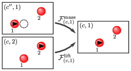
Figure 1: Mass flow (from $(c^{\prime\prime},1)$) and lifting flow (from $(c,2)$) into a lifted configuration $(c,1)$, corresponding to an accepted and a rejected particle move, respectively (see eq. (26)). The total flow should equal the Boltzmann weight $\pi(c)$ in order to satisfy the global balance condition of eq. (22).

In ECMC, any physical configuration $c$ (that is, any set of particle coordinates) is augmented (or “lifted”Chen, Lovász, and Pak (1999)) to include a so-called lifting variable describing which particle is “active”:

$$c\equiv\{\mathbf{r}_{1},\ldots,\mathbf{r}_{N}\}\mapsto(c,a).$$ (23)

In principle, the Boltzmann weight now depends on $a$, but, for simplicity, we require $\pi[(c,a)]=\pi(c)/N$ and absorb the normalization factor $1/N$ into the zero of the potential and omit it in the following.

In ECMC, furthermore, the particle $a$ (the active particle) remains active for subsequent moves as long as they are accepted, and the displacement (in the case that we will treat) is always the same . For simplicity of notation, in the following, the displacement ${\eta}$ is applied in the $\hat{\mathbf{e}}_{x}$ direction for all moves so that the position $\mathbf{r}_{a}$ is updated to $\mathbf{r}_{a}+{\eta}\hat{\mathbf{e}}_{x}$ for accepted moves. When a displacement $\mathbf{r}_{a}\to\mathbf{r}_{a}+{\eta}\hat{\mathbf{e}}_{x}$ is rejected by a target particle $t$, the state of the lifted Markov chain changes in the augmented space as

$$(c,a)\to(c,t),$$ (24)

but the physical configuration $c$ remains unchanged. Liftings thus replace rejections. The global-balance condition must be written in terms of the augmented configurations, and the probability flow $\mathcal{F}_{(c,a)}$ into each lifted configuration $(c,a)$ is then given by the sum of the mass flow $\mathcal{F}^{\text{mass}}_{(c,a)}$, that is, flow corresponding to a particle displacement, and the lifting flow $\mathcal{F}^{\text{lift}}_{(c,a)}$. This sum must equal the statistical weight of $(c,a)$ that, as discussed, equals $\pi(c)$:

$$\mathcal{F}_{(c,a)}=\mathcal{F}^{\text{mass}}_{(c,a)}+\mathcal{F}^{\text{lift}}_{(c,a)}=\pi(c).$$ (25)

In order to assure irreducibility of the Markov chain, one may change the direction of motion, most simply by selecting from the set $\{\hat{\mathbf{e}}_{x},\hat{\mathbf{e}}_{y},\hat{\mathbf{e}}_{z}\}$ in a way that does not need to be random (see the discussion in Section V.2). In ECMC, the process in between two changes of direction is the eponymous “event chain”. The length $\ell$ of an event chain (the cumulative sum of the displacements), and the distribution of $\ell$ are essential parameters for the performance of the algorithm.

To demonstrate that ECMC satisfies the global balance condition, and to study the conditions on the lifting probabilities, we first consider a system of two particles $\{1,2\}$. We may suppose, without restriction, that the active particle is $1$  so that, at a given time, the lifted configuration is $(c,1)$. This lifted configuration can only be reached from two other lifted configurations, one that differs in the configuration variable, and the other in the lifting variable (see Fig. 1). The lifted configurations and the corresponding flows are:

$$\leavevmode\hbox to97.08pt{\vbox to123.28pt{\text{[drawing]}}}. {(c^{\prime\prime},1)} {(c,1)} {(c,2)} {(c^{\prime},2)} \scriptstyle\mathcal{F}^{\text{mass}}_{(c,1)} \scriptstyle\mathcal{F}^{\text{lift}}_{(c,1)} \scriptstyle\mathcal{F}^{\text{mass}}_{(c^{\prime},2)} {(c^{\prime\prime},1)} {(c,1)} {(c,2)} {(c^{\prime},2)} \scriptstyle\mathcal{F}^{\text{mass}}_{(c,1)} \scriptstyle\mathcal{F}^{\text{lift}}_{(c,1)} \scriptstyle\mathcal{F}^{\text{mass}}_{(c^{\prime},2)}$$ (26)

where $c=\{\mathbf{r}_{1},\mathbf{r}_{2}\}$, $c^{\prime\prime}=\{\mathbf{r}_{1}-{\eta}\hat{\mathbf{e}}_{x},\mathbf{r}_{2}\}$, and $c^{\prime}=\{\mathbf{r}_{1},\mathbf{r}_{2}+{\eta}\hat{\mathbf{e}}_{x}\}$. The mass flow of the lifted algorithm from $(c^{\prime\prime},1)$ to $(c,1)$ equals the total Metropolis flow from the nonlifted configuration $c^{\prime\prime}$ to $c$. Because of detailed balance, the latter equals the (nonlifted) Metropolis flow from $c$ to $c^{\prime\prime}$, so that:

$$\mathcal{F}^{\text{mass}}_{(c,1)}=\underbrace{\mathcal{F}^{\text{Met}}_{c^{\prime\prime}\to c}=\mathcal{F}^{\text{Met}}_{c\to c^{\prime\prime}}}_{\text{see eq.~{}\eqref{equ:DetBalMet} }}=\pi(c)p^{\text{Met}}(c\to c^{\prime\prime}).$$ (27)

The lifting flow in eq. (26) equals the rejection probability of the Metropolis move $c\to c^{\prime}$. Because of translational invariance ($c^{\prime\prime}$ is a translated version of $c^{\prime}$), it agrees with the Metropolis rejection probability of the move back from $c$ to $c^{\prime\prime}$:

$$\mathcal{F}^{\text{lift}}_{(c,1)}=\pi(c)\left[1-p^{\text{Met}}(c\to c^{\prime})\right]\\ =\pi(c)\left[1-p^{\text{Met}}(c\to c^{\prime\prime})\right].$$ (28)

$\mathcal{F}^{\text{mass}}_{(c,1)}$ and $\mathcal{F}^{\text{lift}}_{(c,1)}$ thus add up to the Boltzmann weight $\pi(c)$, and global balance is satisfied. The validity of the lifted algorithm (which only satisfies global balance, but breaks detailed balance) hinges on the fact that the underlying Metropolis algorithm satisfies detailed balance and on the translation invariance of the system.

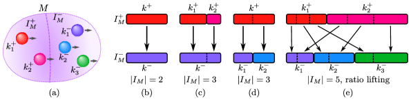
Figure 2: Factors and lifting schemes. (a): A factor $M$ consisting of $|I_{M}|=5$ particles, split into non-empty sets $I_{M}^{+}$ (particles that increase the factor potential) and $I_{M}^{-}$ (see eqs (30) and (31)). (b–e): Lifting schemes. Unit branching $\gamma_{k^{+}\to k^{-}}=1$ and $\gamma_{k^{+}_{1}\to k^{-}}=1,\gamma_{k^{+}_{2}\to k^{-}}=1$ for a pair-particle factor ((b)) and a three-partice factor with $|I_{M}^{-}|=1$ ((c)), and “ratio” lifting scheme for $|I_{M}|=3,|I_{M}^{+}|=1$ ((d)) and for $|I_{M}|>3$ ((e), see eq. (40)).

In the infinitesimal limit, for $N$ particles and a particle-pair factorized potential, the total probability flow into a lifted configuration $(c,a)$ has up to $N$ components, namely $N-1$ lifting flows from $(c,k)$ to $(c,a)$ for $k\neq a$ and one mass move from $(c^{\prime},a)$ to $(c,a)$, where $c^{\prime}$ is again the nonlifted configuration with $x_{a}$ replaced by $x_{a}-\mathrm{d}x$. This corresponds to one lifting flow $\mathcal{F}^{\text{lift}}(k\to a)$ equivalent to that in eq. (26) per target particle $k\neq a$, and a mass flow that is the infinitesimal analogue of that in eq. (26). Furthermore, a particle-pair potential may be further factorized according to multiple factor types $T_{M}$; there then exist $N-1$ lifting flows for each factor $M$ consisting of two particles ($|I_{M}|=2$, with $I_{M}$ the index set of $M$). Of course, factors that do not contain $a$ in their index set do not contribute to this flow.

Factors $M$ with more than two particles ($|I_{M}|>2$) can also be handled within the lifting framework Harland et al. (2017) because, by translational invariance, the sum over the factor derivatives with respect to particle $k$ satisfies:

$$\sum_{k\in I_{M}}\partial_{x_{k}}U_{M}(\{\mathbf{r}_{i}:i\in I_{M}\})=0.$$ (29)

It is useful to separate the particle indices $k\in I_{M}$ of a factor $M$ into two sets $I_{M}^{+}$ (with positive factor derivatives) and $I_{M}^{-}$ (negative factor derivatives) such that:

$$k^{+}\in I_{M}^{+}\Leftrightarrow\quad \partial_{x_{k^{+}}}U_{M}>0$$ (30)

$$k^{-}\in I_{M}^{-}\Leftrightarrow\quad \partial_{x_{k^{-}}}U_{M}<0,$$ (31)

where the factor derivatives satisfy

$$\sum_{k^{+}\in I_{M}^{+}}\partial_{x_{k^{+}}}U_{M}=-\sum_{k^{-}\in I_{M}^{-}}\partial_{x_{k^{-}}}U_{M}$$ (32)

(see Fig. 2a).

The mass flow into a lifted configuration $(c,k^{+})$ with $k^{+}\in I_{M}^{+}$ by itself satisfies global balance,

$$\mathcal{F}^{\text{mass}}_{(c,k^{+})}=\pi_{M}(c^{\prime\prime})p^{\text{Met}}_{M}(c^{\prime\prime}\to c)\\ =\pi_{M}(c)p^{\text{Met}}_{M}(c\to c^{\prime\prime})=\pi_{M}(c),$$ (33)

so that there can be no additional lifting moves into $(c,k^{+})$. This implies that lifting moves are always of the type $(c,k^{+})\to(c,k^{-})$, that is, from an active particle in $I_{M}^{+}$ to a target particle in $I_{M}^{-}$. In contrast, the mass flow into the configuration $(c,k^{-})$ is smaller than $\pi_{M}(c)$:

$$\mathcal{F}^{\text{mass}}_{(c,k^{-})}=\pi_{M}(c^{\prime\prime})p^{\text{Met}}_{M}(c^{\prime\prime}\to c)\\ =\pi_{M}(c)p^{\text{Met}}_{M}(c\to c^{\prime\prime})\\ =\pi_{M}(c)(1+\underbrace{\beta\partial_{x_{k^{-}}}U_{M}}_{<0\,\text{(see eq.~{}\eqref{equ:MMinusDef})\!\!\!\!\!\!\!\!\!\!\!\!\!\!\!\!\!\!}}\mathrm{d}x).$$ (34)

The total lifting flow into $(c,k^{-})$ comes from all lifted configurations $(c,k^{+})$ with $k^{+}\in I_{M}^{+}$:

$$\mathcal{F}^{\text{lift}}_{(c,k^{-})}=\pi_{M}(c)\beta\sum_{k^{+}\in I_{M}^{+}}\partial_{x_{k^{+}}}U_{M}\mathrm{d}x\gamma_{k^{+}\to k^{-}},$$ (35)

where $\gamma_{k^{+}\to k^{-}}$ is the lifting probability from $k^{+}$ to $k^{-}$ once the displacement of $k^{+}$ has been rejected. In order for global balance to hold, eqs (34) and (35) must add up to $\pi(c)$ for all $k^{-}\in M^{-}$. Therefore, and for the algorithm to be rejection-free, one needs Harland et al. (2017):

$$\forall k^{-}\in I_{M}^{-}:\underbrace{\partial_{x_{k^{-}}}U_{M}}_{<0}+\!\!\sum_{k^{+}\in I_{M}^{+}}\underbrace{\partial_{x_{k^{+}}}U_{M}}_{>0}\gamma_{k^{+}\to k^{-}} =0,$$ (36)

$$\forall k^{+}\in I_{M}^{+}:\sum_{k^{-}\in I_{M}^{-}}\gamma_{k^{+}\to k^{-}} =1.$$ (37)

Eqs (36) and (37) can be visualized as $|I_{M}^{+}|$ intervals of length $\partial_{x_{k^{+}}}U_{M}$ placed on the upper row of a two-row table, and of $|I_{M}^{-}|$ intervals of length $|\partial_{x_{k^{-}}}U_{M}|$ on the lower row (see Fig. 2b-e). The total lengths of the two rows are equal (see eq. (32)), and $\gamma_{k^{+}\to k^{-}}$ is the fraction of the interval $k^{+}$ on the upper row that lifts into $k^{-}$ on the lower row. Eq. (36) describes a conservation of the interval lengths from the upper row to the lower row.

For a pair factor ($|I_{M}|=2$), each row has one element, and the lifting is unique ($\gamma=\gamma_{k^{+}\to k^{-}}=1$, see Fig. 2b). For a three-particle factor ($|I_{M}|=3$), if $|I_{M}^{+}|=2$, again clearly $\gamma_{k^{+}\to k^{-}}=1$ for each one of the particles $k^{+}\in I_{M}^{+}$ (see Fig. 2c). If $|I_{M}^{+}|=1$ and $|I_{M}^{-}|=2$, then eq. (36) yields the unique branching probabilities Harland et al. (2017) from $a$ to $k^{-}_{1}$ and $k^{-}_{2}$:

$$\gamma_{k^{+}\to k^{-}_{1}} =-\frac{\partial_{x_{k^{-}_{1}}}U_{M}}{\partial_{x_{k^{+}}}U_{M}}\propto|\partial_{x_{k^{-}_{1}}}U_{M}|,$$ (38)

$$\gamma_{k^{+}\to k^{-}_{2}} =-\frac{\partial_{x_{k^{-}_{2}}}U_{M}}{\partial_{x_{k}^{+}}U_{M}}\propto|\partial_{x_{k^{-}_{2}}}U_{M}|,$$ (39)

which is readily understood from Fig. 2d. Analogously, for factors with $|I_{M}|>3$, the “ratio” lifting corresponds to cutting up each element in the upper row of the table into pieces of length proportional to the elements in the lower row so that

$$\gamma_{k^{+}\to k^{-}}=\frac{\left|\partial_{x_{k^{-}}}U_{M}\right|}{\sum_{k^{-}\in I_{M}^{-}}\left|\partial_{x_{k^{-}}}U_{M}\right|}$$ (40)

(see Fig. 2e). For factors with more than three particles ($|I_{M}|>3$), the “ratio” lifting scheme is not unique Harland et al. (2017). We will make use of this freedom, in Sections IV and V, for factors with up to six particles corresponding to the atoms of two H₂O molecules.

II.3 Event-driven and cell-veto methods

The implementation of ECMC differs notably from that of the Metropolis algorithm, both because of the continuous-time nature of the Markov chain, which can be simulated without approximations using the event-driven approach Peters and de With (2012), and because of the consensus property, which can be checked in $\mathcal{O}(1)$ operations via the cell-veto method, even for infinite-ranged interactions Kapfer and Krauth (2016). It is these two features that we explore in the present section. The intent is to overcome the limitations of time-driven ECMC which considers a finite move ${\eta}\hat{\mathbf{e}}_{x}$ of the active particle:

$$\{\mathbf{r}_{1},\ldots,\mathbf{r}_{a},\ldots,\mathbf{r}_{N}\}\to\{\mathbf{r}_{1},\ldots,\mathbf{r}_{a}+\eta\hat{\mathbf{e}}_{x},\ldots,\mathbf{r}_{N}\}.$$ (41)

This move is either accepted (and then repeated) or it leads to a rejection (by a factor $M\in\mathcal{M}$ containing particle $a$), and it gives rise to a lifting (or possibly to multiple simultaneous liftings). The complexity of time-driven ECMC is $\mathcal{O}(|\{M:a\in I_{M}\}|)$ per displacement ${\eta}\hat{\mathbf{e}}_{x}$. Time-driven ECMC has a discretization error, as it becomes inconsistent if more than one factor simultaneously rejects the move in eq. (41). The parameter ${\eta}$ must be small enough for multiple rejections to be rare. Time-driven ECMC is thus slow, especially for long-ranged interactions, and inexact. It is useful only for testing.

The finite-move ECMC can be implemented as an event-driven, rather than as a time-driven, algorithm Peters and de With (2012); Bortz, Kalos, and Lebowitz (1975), and because all factors are independent, we may consider a single one of them. In the above time-driven ECMC, if the move in eq. (41) (the first move, $m=1$) is accepted, another displacement of magnitude ${\eta}$ is attempted. The $l$th move is:

$$\{\mathbf{r}_{1},\ldots,\mathbf{r}_{a}+(l-1){\eta}\hat{\mathbf{e}}_{x},\ldots,\mathbf{r}_{N}\}\\ \to\{\mathbf{r}_{1},\ldots,\mathbf{r}_{a}+l{\eta}\hat{\mathbf{e}}_{x},\ldots,\mathbf{r}_{N}\}.$$ (42)

After $m-1$ acceptances, finally, the $m$th such move is rejected (and leads to a lifting). The parameter $m$ is itself a random variable distributed with a factor-dependent probability

$$p_{M}(m)=\underbrace{\prod_{l=1}^{m-1}\mathrm{e}^{-\beta\,\Delta U_{M}^{+}(l)}}_{\text{accepted; see eq.~{}\eqref{equ:AcceptanceFactors}}}\overbrace{\left[1-\mathrm{e}^{-\beta\,\Delta U_{M}^{+}(m)}\right]}^{\text{move $m$ rejected}},$$ (43)

where $\,\Delta U_{M}^{+}(l)$ is the change $\,\Delta U_{M}^{+}$ corresponding to the $l$th move in eq. (42). The variable $m$ can be sampled from eq. (43), and the move $\mathbf{r}_{a}\to\mathbf{r}_{a}+(m-1){\eta}\hat{\mathbf{e}}_{x}$ accepted in one step. Although the right-hand side of eq. (43), gives a probability distribution for the displacement of the active particle $a$, it only depends on the positive increments of the factor potential. In the continuum limit ${\eta}\to 0$, the second term on the right-hand side becomes $\beta\mathrm{d}\,U_{M}^{+}(\mathbf{r}_{a}+{\eta}_{M}\hat{\mathbf{e}}_{x})$, that is, the factor event rate of eq. (20), where ${\eta}_{M}$ is the total displacement before a rejection by factor $M$ takes place. In this limit, the exponent in the first term on the right-hand side contains the integral of the factor event rate for the displacement of $\mathbf{r}_{a}$ between $0$ and $\eta_{M}$. This gives the probability density Peters and de With (2012):

$$p_{M}(\,U_{M}^{+})=\beta\exp\left(-\beta\,U_{M}^{+}\right).$$ (44)

In eq. (44), the exponential distribution is sampled by:

$$\beta\,U_{M}^{+}=-\log\left\{\operatorname{ran}_{M}\!\left(0,1\right)\right\},$$ (45)

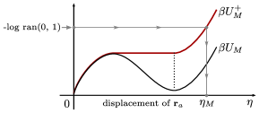
Figure 3: Event-driven ECMCPeters and de With (2012) for a two-particle factor $M$. The integral of the factor derivative multiplied with $\beta$ equals $\beta U_{M}$, whereas the integral of the event rate (in red) must equal $\beta\,U_{M}^{+}$, which is sampled from eq. (45). The calculation of the displacement ${\eta}_{M}$ from the sampled value of $\beta\,U_{M}^{+}=-\log\!\,\operatorname{ran}\!\left(0,1\right)$ is indicated by arrows.

where

$$\underbrace{\beta\,U_{M}^{+}(\mathbf{r}_{a}+{\eta}_{M}\hat{\mathbf{e}}_{x})}_{\text{sampled via eq.~{}\eqref{equ:SampleEta}}}\\ =\int_{0}^{{\eta}_{M}}\underbrace{\beta\left[\partial_{x_{a}}U_{M}(\{\mathbf{r}_{a}+{\eta}\hat{\mathbf{e}}_{x},\mathbf{r}_{k}:k\in I_{M}\})\right]^{+}}_{\text{factor event rate, see eq.~{}\eqref{equ:DiffUEvRate}}}\mathrm{d}{\eta}.$$ (46)

In other words, $\beta\,U_{M}^{+}$ is the cumulative event rate of eq. (20). Eq. (46) is an implicit relation for the limiting displacement ${\eta}_{M}$ at which the rejection takes place as a function of the sampled value of $\beta\,U_{M}^{+}$. For a two-particle factor $M=\left(\{a,k\},\text{pair}\right)$, the integration of the pair event rate in eq. (46) consists in the replacement of the potential $U_{M}$ by a related potential which is zero at $\mathbf{r}_{a}$, and where all the negative increments are replaced by horizontal lines (see Fig. 3).

As mentioned, the factors are independent, and each concerned factor $M$ provides a value ${\eta}_{M}$. The next event takes place at

$${\eta}=\min_{M:a\in I_{M}}{\eta}_{M}$$ (47)

and the factor which realizes this minimum (that is, ${\eta}$)

$$\text{argmin}_{M:a\in I_{M}}{\eta}_{M}$$ (48)

is the one in which the lifting takes place. For a continuous potential, this factor is uniquely defined, and possible simultaneous events, due to finite-precision arithmetic, are too rare to play a role.

The integration of the factor event rate in eq. (46) can be tedious if it cannot be cast into an explicit analytical form. This will for example be the case for the Coulomb potential in the merged-image framework of Section III.3. In addition, the inversion of the factor potential (the computation of ${\eta}_{M}$ in eq. (46)) can be non-trivial. Finally, this calculation must in principle be redone for all the factors that contain the active particle $a$. For a long-ranged potential, this requires $\mathcal{O}(N)=\mathcal{O}(|\{M\in\mathcal{M}:i\in I_{M}\}|)$ event-rate integrations and inversions per event. The cell-veto algorithm Kapfer and Krauth (2016), by use of a comparison function, avoids the integration and the inversion of the event rate, and it moreover reduces the overall complexity of ECMC to $\mathcal{O}(1)$ per event.

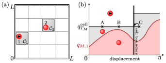
Figure 4: Cell-veto algorithm for a two-particle factor $M$. (a): Active particle $1$ in cell $\mathcal{C}_{1}$ and target particle $2$  in cell $\mathcal{C}_{2}$. (b): The event-rate $q_{M,1}(\mathbf{r}_{1},\mathbf{r}_{2})$ is bounded from above by the cell-event rate $q^{\text{cell}}_{T_{M}}(\mathcal{C}_{1},\mathcal{C}_{2})$, which can be sampled trivially. A cell event may either be rejected (at point “A”) or confirmed (at point “B”) as a particle event (see eq. (50)), while a cell event taking place outside $\mathcal{C}_{1}$ (at point “C”) means that the active particle $1$ will be advanced towards the cell boundary.

We again first consider a pair factor $\left(\{1,2\},\text{pair}\right)$, with $1$ the active particle. The lifted position is $(c,1)$ (with $c=(\mathbf{r}_{1},\mathbf{r}_{2})$) and the displacement is again in direction $\hat{\mathbf{e}}_{x}$ (as in the situation in Fig. 1). We embed the two particles in disjoint cells $\mathcal{C}_{1}$ and $\mathcal{C}_{2}$ (see Fig. 4). The potentials that we consider here are singular only at $\mathbf{r}_{1}=\mathbf{r}_{2}$, so that the event rate for factor $M$ may be bounded by a constant “cell-event” rate $q^{\text{cell}}_{T_{M}}(\mathcal{C}_{1},\mathcal{C}_{2})$:

$$q_{M,1}(\mathbf{r}_{1},\mathbf{r}_{2})\leq q^{\text{cell}}_{T_{M}}(\mathcal{C}_{1},\mathcal{C}_{2})\quad\forall\mathbf{r}_{1}\in\mathcal{C}_{1},\mathbf{r}_{2}\in\mathcal{C}_{2},$$ (49)

where the right-hand side only depends on the factor type. This factor-type dependence may take into account separate cell schemes that could for example correspond to Coulomb interactions between isolated charges, dipole–dipole interactions, or to the Lennard-Jones potential. (We recall that we do not differentiate the different Coulomb types for $2,4,6$ particles to ease notation.) In this work, the condition $\mathcal{C}_{1}\neq\mathcal{C}_{2}$ is adequate to ensure a reasonable value of the cell-event rate. In other cases Kapfer and Krauth (2016), one must exclude a local set of cells, and treat local neighbors outside the cell-veto framework. Cell-event rates are easily tabulated in advance of the ECMC computation proper.

The probability of the event taking place for an infinitesimal displacement $\mathrm{d}x$ equals $q_{M,1}(\mathbf{r}_{1},\mathbf{r}_{2})\mathrm{d}x$. Since

$$q_{M,1}(\mathbf{r}_{1},\mathbf{r}_{2})\mathrm{d}x=\underbrace{q^{\text{cell}}_{T_{M}}(\mathcal{C}_{1},\mathcal{C}_{2})\mathrm{d}x}_{\text{infinitesimal}}\underbrace{\frac{q_{M,1}(\mathbf{r}_{1},\mathbf{r}_{2})}{q^{\text{cell}}_{T_{M}}(\mathcal{C}_{1},\mathcal{C}_{2})}}_{\lesssim 1},$$ (50)

the event can initially be sampled as a “cell event” with the constant infinitesimal probability $q^{\text{cell}}_{T_{M}}(\mathcal{C}_{1},\mathcal{C}_{2})\mathrm{d}x$, before being confirmed with the finite probability $q_{M,1}(\mathbf{r}_{1},\mathbf{r}_{2})/q^{\text{cell}}_{T_{M}}(\mathcal{C}_{1},\mathcal{C}_{2})\leq 1$. We may suppose that the cell event takes place at a lifted configuration $(c^{\prime},1)$ with

$$c^{\prime} =(\mathbf{r}_{1}+\eta\hat{\mathbf{e}}_{x},\mathbf{r}_{2})$$ (51)

$$\pi(\eta) =\exp\left[-\eta q^{\text{cell}}_{T_{M}}(\mathcal{C}_{1},\mathcal{C}_{2})\right],$$ (52)

where $$\eta$$ can be sampled via

$$\eta =-\log\left[\operatorname{ran}\!\left(0,1\right)\right]/q^{\text{cell}}_{T_{M}}(\mathcal{C}_{1},\mathcal{C}_{2}).$$ (53)

Three outcomes are possible for the sampled values of ${\eta}$ and the subsequent confirmation step. First, the cell event may correspond to a configuration $c^{\prime}$ (in eq. (51)) that is already outside the active-particle cell ($c^{\prime}\not\in\mathcal{C}_{1}$). In this case, the move is $(c,1)\to(c^{\prime\prime},1)$, where $c^{\prime\prime}$ is the configuration intersecting the trajectory of particle $1$ with the boundary of $\mathcal{C}_{1}$. Such a cell-boundary event moves the particle, but does not trigger a lifting. Second, the cell event may take place at a configuration $c^{\prime}\in\mathcal{C}_{1}$ but fail to be confirmed as an event (because a uniform random number $\operatorname{ran}\!\left\{0,q^{\text{cell}}_{T_{M}}(\mathcal{C}_{1},\mathcal{C}_{2})\right\}>q_{M,1}(\mathbf{r}_{1},\mathbf{r}_{2})$) (see the second term on the right-hand side of eq. (50)). In this case, the move is $(c,1)\to(c^{\prime},1)$ and no lifting takes place. Third, a cell event may take place at a position $c^{\prime}\in\mathcal{C}_{1}$ and it is confirmed as an event. This event induces a lifting $(c^{\prime},1)\to(c^{\prime},2)$ (see Fig. 4b). In this whole process, the factor derivative $\tilde{q}_{M,1}$ is evaluated only when a cell event is triggered from the exponential distribution in eq. (52). The costly integration of the factor event rate in eq. (46) is thus avoided.

For an $N$-particle system, the cell-veto algorithm organizes the search of the next lifting in $\mathcal{O}(1)$ operations. It suffices to choose a regular grid of cells such that, normally, only a single particle belongs to each cell. (Exceptional double-cell occupancies can be handled easily Kapfer and Krauth (2016).) In this case, the total event rate with respect to factor type $T_{M}$ for an active particle in $\mathcal{C}_{a}$ is bounded by the total cell event rate

$$Q^{\text{cell}}_{T_{M}}(\mathcal{C}_{a})=\sum_{\text{cells}\ \mathcal{C}_{t}\neq\mathcal{C}_{a}}q^{\text{cell}}_{T_{M}}(\mathcal{C}_{a},\mathcal{C}_{t}).$$ (54)

In a translationally invariant system, the total cell event rate does not depend on the active cell, so that $Q^{\text{cell}}_{T_{M}}(\mathcal{C}_{a})\equiv Q^{\text{cell}}_{T_{M}}$, a constant that is computed before the ECMC simulation starts from the total number of cells that scales as $\mathcal{O}(N)$. The next cell event is obtained from an exponential distribution with parameter $Q^{\text{cell}}_{T_{M}}(\mathcal{C}_{a})$. This event corresponds to cell $\mathcal{C}_{t}$ with probability $\propto q^{\text{cell}}_{T_{M}}(\mathcal{C}_{a},\mathcal{C}_{t})$, posing a discrete sampling problem that can be solved in $\mathcal{O}(1)$ by Walker’s algorithm Walker (1977); Kapfer and Krauth (2016).

The cell-veto algorithm samples the Boltzmann distribution without performing the event-rate integration in eq. (46). It requires only $\mathcal{O}(1)$ factor-potential evaluations per event in an $N$-particle system. As a consequence, the total potential of eq. (1) is not updated and the potential remains unknown as the Markov chain evolves. This is what sets ECMC apart from traditional simulation approaches.

III ECMC Coulomb algorithms

In a three-dimensional simulation box with periodic boundary conditions, the Coulomb potential is only conditionally convergent for a charge-neutral system, and it is infinite for a system with a net charge. Finiteness of the potential can be recovered in both cases if each point charge is compensated by a background charge distribution. Traditionally, this is chosen as uniform within the simulation box de Leeuw, Perram, and Smith (1980). The precise association of each background charge with its point charge is not unique. This leads to different electrostatic boundary conditions, which are linked to the polarization state of the simulation box. Consistency imposes a distinct fluctuation theoremde Leeuw, Perram, and Smith (1980) for each choice of boundary condition when computing macroscopic physical properties such as the dielectric constant. Alternatively to the uniform compensating background charge, in ECMC, a line-charge model was introduced Kapfer and Krauth (2016). In this model, the background charge distribution is one-dimensional and the factor derivatives are absolutely convergent. The potential for different variants of the line-charge model can be absolutely or conditionally convergent.

As discussed in Section II.1, ECMC allows for different Coulomb factor sets, that may influence the convergence properties of the algorithm, although the steady state is invariably given by the Boltzmann distribution. Roughly, there are two inequivalent Coulomb factorizations Kapfer and Krauth (2016). Firstly, the periodic two-particle problem can be embedded on a three-dimensional torus and the potential merged from all the topologically inequivalent minimal paths between particles (see Fig. 5a). For two particles, $\{1,2\}$, this “merged-image” system has a single factor $\left(\{1,2\},\,\text{Coulomb}\right)$. For $N$ particles, this gives the factor set

$$\{\left(\{i,j\},\,\text{Coulomb}\right):i<j\in\{1,\ldots,N\}\}.$$ (55)

In general, the merged-image factors may comprise more than two particles, but they do not distinguish between the different images of a local configuration (for example an H₂O molecule). Secondly, we may picture the three-dimensional periodic system as an infinite number of periodic images of the simulation box indexed by an integer vector $\mathbf{n}\in\mathbb{Z}^{3}$. For two particles already, this “separate-image” system has an infinite number of factors and for $N$ particles, the factor set is

$$\{\left(\{i,j\},\,\text{Coulomb}_{\mathbf{n}}\right):i<j\in\{1,\ldots,N\},\mathbf{n}\in\mathbb{Z}^{3}\}.$$ (56)

More generally, an individual “separate-image” factor may describe an image of certain particles inside the simulation box.

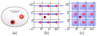
Figure 5: Periodic two-particle Coulomb system. (a): Toroidal representation corresponding to a merged-image factor. (b): Line-charge representation. The target point-charge particle and each of its copies are compensated by line charges of length $2L$. The active particle inside the central simulation box $[0,L)^{3}$ is not replicated. (c): Compensating volume-charge representation corresponding to “tin-foil” boundary conditions.

The aim of this section is threefold. First, we present the tin-foil and the line-charge Coulomb formulations and then demonstrate that, although the potentials differ, the Coulomb factor derivatives (that for pair factors yield the event rates) are identical. Second, we discuss two efficient algorithms for the merged-image Coulomb derivatives of a pair of particles, one algorithm from the tin-foil perspective and the other summing up line-charge derivatives. Third, we set up an ECMC simulation for two particles in a periodic three-dimensional simulation box in order to validate that the merged-image and the separate-image factor sets indeed show indistinguishable equilibrium properties. We then discuss possible applications for both factorizations.

III.1 Tin-foil electrostatics within ECMC

The traditional treatment of electrostatic interactions with periodic boundary conditions is based de Leeuw, Perram, and Smith (1980) on a large spherical aggregate of images of the three-dimensional cubic simulation box. The polarization state of the simulation box is expressed through electrostatic boundary conditions. With “tin-foil” boundary conditions, the potential of $N$ particles $i\in\{1,\ldots,N\}$ of charge $c_{i}$ (in units where the Coulomb potential between two point charges in free space is $U_{ij}=c_{i}c_{j}/|\mathbf{r}_{ij}|$), is de Leeuw, Perram, and Smith (1980):

$$U_{\text{C}}(\{\mathbf{r}_{1},\ldots,\mathbf{r}_{N}\},\{c_{1},\ldots,c_{N}\})\\ =\frac{1}{2}\sum_{i=1}^{N}c_{i}\psi(\mathbf{r}_{i})+U_{\text{self}}(\alpha),$$ (57)

with the electrostatic potential $\psi$:

$$\psi(\mathbf{r}_{i})=\, \sum_{j\neq i=1}^{N}c_{j}\left[\sum_{\mathbf{n}\in\mathbb{Z}^{3}}\frac{{\rm erfc}(\alpha|\mathbf{r}_{ij}+\mathbf{n}L|)}{|\mathbf{r}_{ij}+\mathbf{n}L|}\right.$$

$$\left.+\frac{4\pi}{L^{3}}\sum_{\mathbf{q}\neq(0,0,0)}\frac{\mathrm{e}^{-\mathbf{q}^{2}/(4\alpha^{2})}}{\mathbf{q}^{2}}\cos\left(\mathbf{q}\cdot\mathbf{r}_{ij}\right)\right],$$ (58)

where the Fourier-space sum is over $\mathbf{q}=2\pi\mathbf{m}/L$ with $\mathbf{m}\in\mathbb{Z}^{3}$. The self-energy contribution $U_{\text{self}}(\alpha)$ is independent of the particle positions, and drops out of our considerations, which are only concerned with derivatives of the potential. The left-hand side of eq. (57) is independent of the convergence factor $\alpha>0$, which however influences the speed of evaluation of eq. (58). Direct evaluation of the sums for $N$ point charges leads to an optimal choice $\alpha\sim N^{1/6}/L$, and a scaling in operations $\mathcal{O}(N^{3/2})$. The Particle–Mesh Ewald method uses an interpolating mesh to approximate the Fourier sum, leading to $\mathcal{O}(N\log{N})$ operations to evaluate the potential. In merged-image ECMC we only use eq. (58) for $N=2$ with $\alpha=\mathcal{O}(1/L)$, and evaluate the derivative of the Coulomb potential to machine precision with $\mathcal{O}(1)$ effort.

We continue, as in Section II.2, with a two-particle factor $\left(\{1,2\},\,\text{\text{Coulomb}}\right)$. The tin-foil factor derivative is given by:

$$\tilde{q}_{\left(\{1,2\},\,\text{\text{Coulomb}}\right),1}(\mathbf{r}_{12},\{c_{1},c_{2}\})\\ =\tilde{q}_{\text{Real}}(\mathbf{r}_{12})+\tilde{q}_{\text{Four.}}(\mathbf{r}_{12}),$$ (59)

with the real-space derivative $\tilde{q}_{\text{real}}$

$$\tilde{q}_{\text{real}}(\mathbf{r}_{12})= c_{1}c_{2}\sum_{\mathbf{n}\in\mathbb{Z}^{3}}\frac{\mathbf{r}_{12}+n_{x}L}{|\mathbf{r}_{12}+\mathbf{n}L|^{2}}\left[\frac{{\rm erfc(\alpha|\mathbf{r}_{12}+\mathbf{n}L|)}}{|\mathbf{r}_{12}+\mathbf{n}L|}\right.$$

$$\left.+\frac{2\alpha\mathrm{e}^{-\alpha^{2}|\mathbf{r}_{12}+\mathbf{n}L|^{2}}}{\pi^{1/2}}\right],$$ (60)

and the Fourier-space derivative $\tilde{q}_{\text{Four.}}$

$$\tilde{q}_{\text{Four.}}(\mathbf{r}_{12})= c_{1}c_{2}\frac{4\pi}{L^{3}}\sum_{\mathbf{q}\neq 0}q_{x}\frac{\mathrm{e}^{-\mathbf{q}^{2}/(4\alpha^{2})}}{\mathbf{q}^{2}}\sin\left(\mathbf{q}\cdot\mathbf{r}_{12}\right).$$ (61)

For two particles and, more generally, for pair factors in an $N$-particle system, the merged-image Coulomb pair-event rate, from eq. (59), is given by:

$$q_{\left(\{1,2\},\,\text{\text{Coulomb}}\right),1}(\mathbf{r}_{12},\{c_{1},c_{2}\})\\ =\beta\left[\tilde{q}_{\left(\{1,2\},\,\text{\text{Coulomb}}\right),1}(\mathbf{r}_{12},\{c_{1},c_{2}\})\right]^{+}.$$ (62)

In Sections IV and V, we will consider dipole–dipole factors with an index set comprising the four or six particles of two molecules and the “Coulomb” type corresponding to all the Coulomb interactions between the two molecules. The factor potential in this case is the sum over Coulomb pairs within the factor, and the factor derivatives needed in eq. (36) are the sum of a finite number of pairwise Coulomb derivatives as in eq. (59). The evaluation of the dipole–dipole factor derivatives remains of complexity $\mathcal{O}(1)$ because the number of elements in each factor remains finite as $N\to\infty$. In ECMC, only a single factor has to be evaluated precisely for each move (see Section II.3) whereas in traditional MCMC or MD computations the Coulomb potential in eq. (57) or its derivatives are computed for all $N$ particles.

III.2 Line-charge model

In a large periodically reproduced aggregate of the simulation box, the sum over the Coulomb derivatives between a charged active particle and multiple target images (without neutralizing backgrounds) is ill-defined. However, the compensating uniform volume charge is not the only option to regularize the sum, as the line-charge model Kapfer and Krauth (2016) and its variants provide alternatives to tin-foil electrostatics. Here, straight lines of charges are associated with each copy of the target particle, and aligned with its direction of motion (in our example $\hat{\mathbf{e}}_{x}$, see Fig. 5b). Although the merged-image line-charge potential, in its simplest version, is itself not absolutely convergent, its factor derivatives are unequivocally defined and equivalent to those obtained with tin-foil boundary conditions. By itself, the line charge neutralizes the charge of the target particle, and (because it is centered) also creates an object with zero dipole moment. Previous work Kapfer and Krauth (2016) used line charges of length $L$. Here, we consider lengths $pL$ with integer $p$ (see Fig. 5b). The line charges are replicated over a cubic lattice indexed by the lattice vector $\mathbf{n}$. Lines of different images meet (see Fig. 5b). The Coulomb potential of the line-charge model naturally differs from the one of the tin-foil model because the background charge distributions are manifestly different. However, the merged-image Coulomb derivative of the line-charge model, relevant to ECMC, is identical to the tin-foil expression.

Explicitly, the contribution to the Coulomb derivative from an image $\mathbf{n}$ (with $\mathbf{n}=(0,0,0)$ the original simulation box) is

$$\tilde{q}_{\left(\{1,2\},\,\text{\text{Coulomb}}_{\mathbf{n}}\right),1}(\mathbf{r}_{12})=c_{1}c_{2}\left\{\frac{\mathbf{r}_{12}+n_{x}L}{|\mathbf{r}_{12}+\mathbf{n}L|^{3}}+\right.\\ \left.\frac{1}{pL}\left[\frac{1}{|\mathbf{r}_{12}+L\left(\mathbf{n}+p\hat{\mathbf{e}}_{x}\right)/2|}-\frac{1}{|\mathbf{r}_{12}+L\left(\mathbf{n}-p\hat{\mathbf{e}}_{x}\right)/2|}\right]\right\}$$ (63)

The line charge generates an electrostatic potential at large separations, $\mathbf{r}=L\mathbf{n}$, which varies with a quadrupolar form. Thus, in any given direction the Coulomb derivative decays as $1/|\mathbf{r}|^{4}$. For this reason, the sum over the images of the Coulomb derivatives of eq. (63) converges absolutely. The merged-image Coulomb derivative, in the line-charge formulation, is thus

$$\overbrace{\tilde{q}_{\left(\{1,2\},\,\text{\text{Coulomb}}\right),1}(\mathbf{r}_{12},\{c_{1},c_{2}\})}^{\text{tin-foil expression, eq.~{}\eqref{equ:CoulombDirectDeriv}}}\\ =\underbrace{\sum_{\mathbf{n}}\tilde{q}_{\left(\{1,2\},\,\text{\text{Coulomb}}_{\mathbf{n}}\right),1}(\mathbf{r}_{12})}_{\text{sum over line charges, eq.~{}\eqref{equ:imagewiseLineChargeDirectDeriv}}}.$$ (64)

To show this, we first consider the target particle $2$ in the simulation box and all its images to be surrounded by a cube of neutralizing charge of volume $L^{3}$ centered on the particle $2$ and its images. This volume-charge model (see Fig. 5c) is closely connected to the the line-charge model (see Fig. 5b). Point charge and associated volume charge have vanishing charge, dipole and quadrupole moments (whereas the line-charge model, in its simplest form, has a finite quadrupole moment). We now compare spherical (radius $R\gg L$) and cubic aggregates (of side $2R$) of target images, and study the electrostatic potential within the central simulation box. In this process, the active particle is not replicated, and it remains within the simulation box. Due to the vanishing quadrupole moment of the volume charges, the difference in the electrostatic potential on the particle $1$ in the spherical and cubic aggregates decreases at least as fast as $1/R^{2}$. However the electrostatic potential in the center of the spherical aggregate corresponds to a zero-polarization state which is identical to the tin-foil expression of eq. (58).

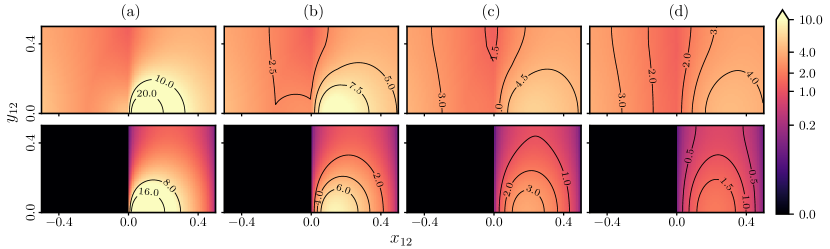
Figure 6: Comparison of the sum of the separate-image event rates $\sum_{\mathbf{n}}\beta\left[\tilde{q}_{\left(\{1,2\},\,\text{\text{Coulomb}}_{\mathbf{n}}\right),1}(\mathbf{r}_{12})\right]^{+}$ (upper row) and the merged-image event rate $\beta\left[\tilde{q}_{\left(\{1,2\},\,\text{\text{Coulomb}}\right),1}(\mathbf{r}_{12})\right]^{+}$ (lower row). In all panels $\mathbf{r}_{12}=(x_{12},y_{12},z_{12})$ with (a): $z_{12}=0.1$, (b): $z_{12}=0.2$, (c): $z_{12}=0.3$, and (d): $z_{12}=0.4$. $L=1$ and $\beta c_{1}c_{2}=1$ throughout.

We now find explicit integral expression for the Coulomb derivative of an aggregate of line charges and volume charges and show that the difference is zero in the limit of a large assembly. We again consider the interaction between an active particle and the cubic aggregate of the ${(2{K}+1)}^{3}$ copies of the target particle (the central simulation box and its images). (The active particle is placed inside the simulation box.) The Coulomb potential between the active particle and a single target particle is

$$U_{12}=4\pi c_{1}\int_{-\infty}^{\infty}\frac{\mathrm{d}^{3}\mathbf{q}}{{(2\pi)}^{3}}\,e^{i{\mathbf{q}}\cdot\mathbf{r}_{12}}\frac{\rho_{2}({\mathbf{q}})}{|\mathbf{q}|^{2}},$$ (65)

where $\rho_{2}({\mathbf{q}})$ is the structure factor of the target particle and the background. We now sum over the images, separated by a multiple of the simulation box size $L$ along each axis. This requires evaluating the sum

$$D_{K}(q_{x})=\sum_{l=-K}^{K}\mathrm{e}^{iq_{x}lL}=\frac{\sin\left[q_{x}L(K+1/2)\right]}{\sin(q_{x}L/2)},$$ (66)

and analogously for $q_{y}$ and $q_{z}$. With the product

$$\tilde{D}_{K}(\mathbf{q})=D_{K}(q_{x})D_{K}(q_{y})D_{K}(q_{z}),$$ (67)

this gives the potential of the active particle in the aggregate of the target particle and its images:

$$U_{K}=4\pi c_{1}\int_{-\infty}^{\infty}\frac{\mathrm{d}^{3}\mathbf{q}}{{(2\pi)}^{3}}\tilde{D}_{K}(\mathbf{q})\,\mathrm{e}^{i{\mathbf{q}}\cdot\mathbf{r}_{12}}\,\frac{\rho_{2}({\mathbf{q}})}{|\mathbf{q}|^{2}}.$$ (68)

Eq. (66) is the Dirichlet kernel which converges, in a weak sense, to a sum of $\delta$-functions in the limit of large $K$:

$$D_{K}(q_{x})\xrightarrow[K\to\infty]{}\frac{2\pi}{L}\sum_{m=-\infty}^{\infty}\delta\left(q_{x}-m\frac{2\pi}{L}\right),$$ (69)

and similarly for $q_{y}$ and $q_{z}$. The width of the central peak of $D_{K}$ scales as $1/K$ for large $K$. Integrals over sufficiently well-behaved objects become summations in the limit of large $K$:

$$\int\frac{\mathrm{d}^{3}\mathbf{q}}{{(2\pi)}^{3}}\tilde{D}_{K}(\mathbf{q})f({\mathbf{q}})\rightarrow\frac{1}{L^{3}}\sum_{{\mathbf{q}}=2\pi{\bf m}/L}f({\mathbf{q}}).$$ (70)

For the volume-charge model, the structure factor is

$$\rho_{2}({\mathbf{q}})=c_{2}\left(1-\operatorname{sinc}\frac{q_{x}L}{2}\operatorname{sinc}\frac{q_{y}L}{2}\operatorname{sinc}\frac{q_{z}L}{2}\right),$$ (71)

where the first term on the right-hand side describes the point charge and the product of cardinal sine functions, $\operatorname{sinc}(q_{x})=\sin(q_{x})/q_{x}$, etc., the uniform background volume charge.

From eqs (68) and (71), the potential of a finite cubic array of images of the particle $2$, with active particle $1$, is

$$U_{K}^{\text{volume}}=c_{1}c_{2}\int\frac{\mathrm{d}^{3}\mathbf{q}}{2\pi^{2}}\tilde{D}_{K}(\mathbf{q})\frac{\mathrm{e}^{i{\mathbf{q}}\cdot{\mathbf{r}_{12}}}}{|\mathbf{q}|^{2}}\\ \times\left(1-\operatorname{sinc}\frac{q_{x}L}{2}\operatorname{sinc}\frac{q_{y}L}{2}\operatorname{sinc}\frac{q_{z}L}{2}\right).$$ (72)

For line charges of length $pL$, we find

$$U_{K}^{\text{line}}=c_{1}c_{2}\!\!\int\frac{\mathrm{d}^{3}\mathbf{q}}{2\pi^{2}}\tilde{D}_{K}(\mathbf{q})\frac{\mathrm{e}^{i{\mathbf{q}}\cdot{\mathbf{r}_{12}}}}{|\mathbf{q}|^{2}}\!\left(1-\operatorname{sinc}\frac{pq_{x}L}{2}\right).$$ (73)

The volume-charge model is equivalent to the tin-foil Coulomb potential. The line-charge model, whose potential is not absolutely convergent, is nevertheless equivalent for ECMC because, as we will see, the integrals in eqs (72) and (73) yield uniquely defined and equivalent Coulomb derivatives for large $K$. The difference between the two is given by:

$$\Delta U_{K}=(U_{K}^{\text{line}}-U_{K}^{\text{volume}})=c_{1}c_{2}\int\,\frac{\mathrm{d}^{3}\mathbf{q}}{2\pi^{2}}\,\tilde{D}_{K}(\mathbf{q})\frac{\mathrm{e}^{i{\mathbf{q}}\cdot{\mathbf{r}_{12}}}}{|\mathbf{q}|^{2}}\\ \times\left(\operatorname{sinc}\frac{q_{x}L}{2}\operatorname{sinc}\frac{q_{y}L}{2}\operatorname{sinc}\frac{q_{z}L}{2}-\operatorname{sinc}\frac{pq_{x}L}{2}\right)$$

The Dirichlet kernels imply that the integral in this equation is dominated by contributions near $\mathbf{q}=2\pi\mathbf{m}/L$. However, the function $\operatorname{sinc}(q_{i}L/2)$ also has zeros at these same points (except when $q_{i}=0$, where the $\operatorname{sinc}$ function is equal to one). For large $K$, the potential differences is thus dominated by a sum over $q_{y}$, $q_{z}$, with $q_{x}=0$. This implies that the potential on the active particle equals (to within a constant) the tin-foil potential for motion parallel to the line-charges, but the difference of potentials is corrugated in the perpendicular $y-z$ plane. This is a consequence of the fusion of multiple aligned line charges into a single uniform line when $p$ is integer (see Fig. 5b).

We examine the derivative of $\Delta U_{K}$ to show that the Coulomb derivatives converge to the same value:

$$\partial_{x_{1}}\Delta U_{K}=\int\,\frac{\mathrm{d}^{3}\mathbf{q}}{2\pi^{2}}\,\tilde{D}_{K}(\mathbf{q})\frac{q_{x}\sin(\mathbf{q}\cdot\mathbf{r}_{12})}{|\mathbf{q}|^{2}}\\ \times\left(\operatorname{sinc}\frac{q_{x}L}{2}\operatorname{sinc}\frac{q_{y}L}{2}\operatorname{sinc}\frac{q_{z}L}{2}-\operatorname{sinc}\frac{pq_{x}L}{2}\right),$$ (74)

which suppresses the contributions which remained for the calculation of the potential, due to the factor $q_{x}\sin(q_{x}x)$ near $q_{x}=0$.

Finally, we consider explicitly the possible divergence at $|\mathbf{q}|=0$ in eq. (74), due to the presence of the term $1/|\mathbf{q}|^{2}$. We expand all the trigonometric functions in the integrand, $\Delta I_{K}$, to find

$$\Delta I_{K}\xrightarrow[\mathbf{q}\rightarrow 0]{}\text{const}\times\frac{q_{x}^{2}\left[(p^{2}-1)q_{x}^{2}-q_{y}^{2}-q_{z}^{2}\right]}{|\mathbf{q}|^{2}}\tilde{D}_{K}(\mathbf{q}).$$

Even this contribution is thus driven to zero for large $K$. We conclude that in a periodic three-dimensional system, the line-charge model becomes equivalent to the volume-charge model, and therefore to tin-foil electrostatics. The line charges must lie parallel to the direction of motion but can of course be switched at will. In contrast, the volume-charge model gives the tin-foil Coulomb derivatives in all directions.

III.3 Algorithms for Coulomb derivatives

The merged-image Coulomb derivatives are best computed from the tin-foil expressions of eq. (62). To accelerate the evaluation, we reduce the Fourier-space component of eq. (61) to a sum over non-negative components $(m_{x},m_{y},m_{z})$:

$$\tilde{q}_{f}(\mathbf{r}_{12})=A_{xyz}\sin(\lambda_{12}^{x})\cos(\lambda_{12}^{y})\cos(\lambda_{12}^{z}),$$ (75)

where $\lambda_{12}^{x}=2\pi m_{x}x_{12}/L$, and similarly in $y$ and $z$ and where

$$A_{xyz}=\frac{16c_{1}c_{2}m_{x}}{L^{2}|\mathbf{m}|^{2}2^{\delta_{m_{y},0}+\delta_{m_{z},0}}}\exp\left(-\frac{\pi^{2}|\mathbf{m}|^{2}}{\alpha^{2}L^{2}}\right)$$ (76)

is a position-independent tensor that can be computed before the simulation starts. In eq. (75), repeated indices $(x,y,z)$ are summed over non-negative integers $(m_{x},m_{y},m_{z})$.

The merged-image Coulomb derivatives can also be computed from the sum of the line-charge derivatives (see the right-hand side of eq. (64)). Because of the symmetry of the line charges, the quadrupolar contribution to the derivative is an odd function of $x$, so that forward and backward terms cancel, and that the sum converges as $1/{K}^{2}$ for large ${K}$. The convergence may be accelerated using Richardson extrapolation Bender and Orszag (1978) (see Fig. 7). Denoting the finite line-charge sum over the range $\mathbf{n}\in[-{K},{K}]^{3}$ as $S_{K}$ and assuming that:

$$S_{{K}}=S_{\infty}+\frac{A}{{K}^{p}},$$ (77)

one may eliminate $A$ as:

$$S^{\prime}_{{K}+1}=\frac{{({K}+1)}^{p}S_{{K}+1}-{{K}^{p}}S_{{K}}}{{({K}+1)}^{p}-{{K}^{p}}}.$$ (78)

The sequence $(S^{\prime}_{{K}+1}-S_{\infty})$ then decays as $1/{K}^{p+1}$. The transformation of eq. (78) can be iterated, each time gaining one power in the asymptotic behavior of the sequence. The merged-image line-charge derivatives converge to the tin-foil expression of eq. (59), confirming that the two algorithms compute the same object and that individual factors in the line-charge model may be used to simulate tin-foil potentials.

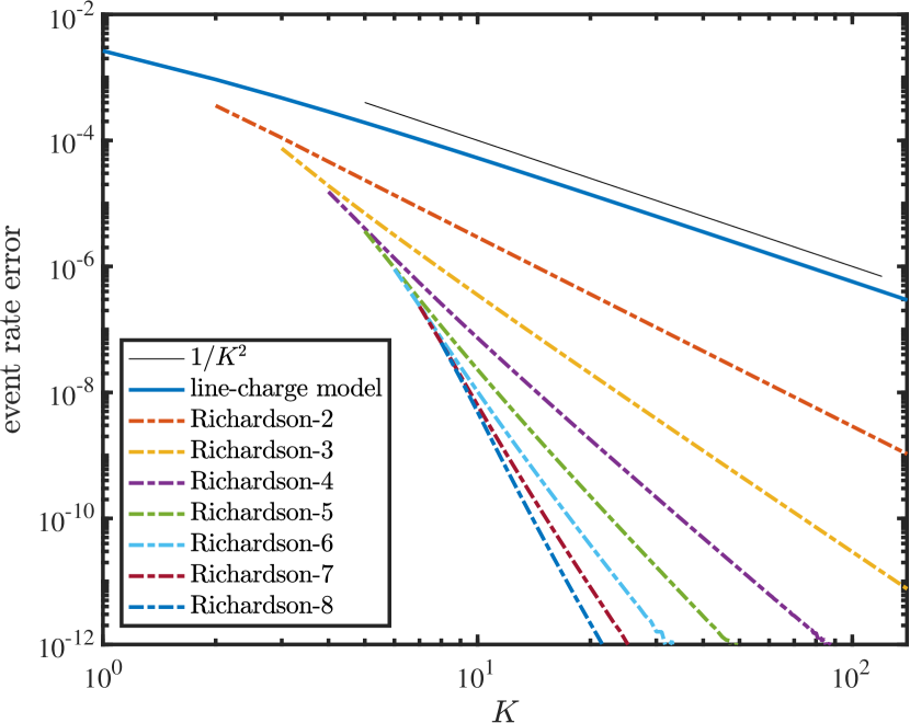
Figure 7: Comparison of the tin-foil expression for the Coulomb factor derivative and the sum over line charges for a given value of $\mathbf{r}_{12}$ (see eq. (64)) as a function of the cutoff ${K}$. The 8-fold iterated Richardson extrapolation for the line-charge expression agrees with the tin-foil expression to within $10^{-12}$ for ${K}\approx 20$.

As in the line-charge model, one may sum up the associated point charges and their compensating volume charges explicitly, rather than proceeding through Fourier transformation. However, the analytic formulas are difficult to work with. A further possibility consists in compensating each point charge with more than one line charge. Remarkably, four line charges arranged on a square of side $L/\sqrt{12}$ in the $y-z$ plane, cancel dipole and quadrupole moments in the multipole expansion and lead to an absolutely converging sum for the electrostatic potential. One may also construct more elaborate sheets and volumes of screening charges to cancel higher orders in the multipole expansion. All of these screening objects presented here regularize the sum of the pair derivatives over images and allow for separate-image factor sets (analogous to eq. (56), see Section III.4). Although the sequence $S_{K}$ decays faster, the Coulomb event rate is not reduced by these different objects.

III.4 Separate-image ECMC

As we have seen, all the Coulomb interactions in a finite system with periodic boundary conditions can be image-merged into a single Coulomb  type that sums over all the inequivalent minimal paths between two points on a torus, and that correspond to images in the rolled-out representation of periodic boundary conditions. For two particles $1$ and $2$, this is expressed through a single factor $M=\left(\{1,2\},\,\text{\text{Coulomb}}\right)$. The corresponding factor derivatives can then be computed with the traditional tin-foil expression (eq. (59)) or within the line-charge framework (eq. (64)). The choice of one over the other is a matter of efficiency only (the algorithmic complexity being the same). Each of the formulations suggest other choices for the interaction types. In the line-charge formulation, the choice of an infinite set of types $\{\,\text{Coulomb}_{\mathbf{n}}:\mathbf{n}\in\mathbb{Z}^{3}\}$ suggests itself. For two particles $1$ and $2$, the set of separate-image factors is $\{\left(\{1,2\},\,\text{Coulomb}_{\mathbf{n}}\right):\mathbf{n}\in\mathbb{Z}^{3}\}$. Within ECMC, these images are statistically independent but only one of them must be computed precisely for each event. This is because, as in Section II, we can use a variant of the cell-veto algorithm (supplemented with an asymptotic bounding function Kapfer and Krauth (2016)), in order to sample the relevant image index $\mathbf{n}$ and to then compute the corresponding factor derivative of $M_{\mathbf{n}}$.

Separate-image Coulomb factors generally come with larger pair event rates, as the contributions from different images do not compensate (see Fig. 6). On the other hand, evaluating a separate-image Coulomb derivative (as in eq. (63)) to machine precision requires just a few operations, many fewer than what is required for its merged-image counterpart. Details of the separate-image Coulomb factors can influence the efficiency of the algorithm. As an example, the terminal point of the line charge is a singular point of eq. (63) and should not approach another point charge in the system. This motivates our choice of length $2L$ (or multiples thereof), as the terminal point of one line charge then coincides with the position of an image of the original particle. For the Coulomb potential, the nonphysical line-charge singularity, confounded with the singularity of the point charge, no longer disrupts the ECMC dynamics.

The dynamic behavior of the different factor sets for the Coulomb problem have not yet been explored in detail. As a first step, for a system of two like Coulomb charges, merged-image and separate-image ECMC was validated against the regular tin-foil Metropolis algorithm (see Fig. 8). All three methods clearly sample the Boltzmann distribution in the asymptotic steady state.

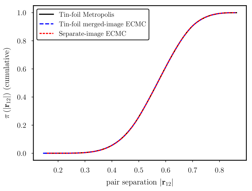
Figure 8: Cumulative histogram of the pair separation $|\mathbf{r}_{12}|$ for two particles of equal charge in a periodic three-dimensional simulation box ($\beta c_{1}c_{2}=2$, $L=1$).

IV Dipole–dipole factors

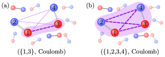
Figure 9: Model of two-particle dipoles. (a): Particle–particle factor associating two point charges that belong to different dipoles. (b): “dipole–dipole” factor comprising four Coulomb interactions.

In ECMC, one may tailor the factor sets to the problems at hand. In electrostatic systems made up of local dipoles, specific “dipole–dipole” Coulomb factors may thus contain all the atoms distributed over two molecules that can be far apart from each other. These factors yield much smaller event rates than “particle–particle” pair factors. In addition, a special “inside-first” lifting scheme can direct most of the lifting flow from the active particle to a target particle situated on the same molecule. Even for a non-local factor made up of two distant dipoles, the lifting flow will thus mostly be between an active particle and a target particle on the same molecule (the probability of an intramolecular lifting grows like $\log\!\,N$, whereas all the intermolecular liftings remain constant). We expect such a local lifting scheme for extended factors to show interesting dynamic properties. In the present section, we explore dipole–dipole factors in a simple model of charge-neutral two-particle molecules before employing them, in Section V, to a model of liquid water. We expect dipole–dipole factors and their variants to have useful applications in ECMC.

Concretely, for a simple model of two-particle dipoles in a three-dimensional periodic simulation box, the dipole–dipole factor for the particles $\{1,2,3,4\}$ is given by:

$$\left(\{1,2,3,4\},\,\text{\text{Coulomb}}\right),$$ (79)

(see Fig. 9b), where the corresponding Coulomb factor potential is:

$$U_{\left(\{1,2,3,4\},\,\text{Coulomb}\right)}(\mathbf{r}_{1},\ldots,\mathbf{r}_{4})\\ =\sum_{i=1}^{2}\sum_{j=3}^{4}U_{\text{C}}(\mathbf{r}_{ij},\{c_{i},c_{j}\}).$$ (80)

The factor of eq. (79) thus comprises the four Coulomb potentials between these particles, using the Coulomb potential of eq. (57). The model excludes, as is usual Wu, Tepper, and Voth (2006), Coulomb interactions within a dipole. For the same four particles, one may also use the “particle–particle” factors

$$\{\left(\{1,3\},\,\text{Coulomb}\right),\left(\{1,4\},\,\text{Coulomb}\right)\\ \left(\{2,3\},\,\text{Coulomb}\right),\left(\{2,4\},\,\text{Coulomb}\right)\},$$ (81)

with the “particle–particle” factor potential:

$$U_{\left(\{i,j\},\,\text{Coulomb}\right)}(\mathbf{r}_{ij},\{c_{i},c_{j}\})=U_{\text{C}}(\mathbf{r}_{ij},\{c_{i},c_{j}\})$$ (82)

(see Fig. 9a). We suppose that the particle $1$ is active. The dipole–dipole event rate

$$\beta\left[\tilde{q}_{\left(\{1,2,3,4\},\,\text{Coulomb}\right),1}\right]^{+}$$ (83)

then allows the interactions $U_{\text{C}}(\mathbf{r}_{13})$ and $U_{\text{C}}(\mathbf{r}_{14})$ to compensate each other (and to give the event rate corresponding to a point charge interacting with a dipole), while the particle–particle event rate

$$\beta\left[\tilde{q}_{\left(\{1,3\},\,\text{Coulomb}\right),1}\right]^{+}+\beta\left[\tilde{q}_{\left(\{1,4\},\,\text{Coulomb}\right),1}\right]^{+}$$ (84)

remains much larger (corresponding to a point charge separately interacting with two isolated point charges), because the unit-ramp functions are both non-negative (see eq. (14)) and one of them is usually zero.

IV.1 Event-rate scaling for Coulomb factors

We now consider a homogeneous system of dipoles of size $|\mathbf{d}|\sim d$ small compared to the simulation box (see Fig. 10). For concreteness, we suppose that particle $1$ is the active particle. The event rate, whose scaling with system size we compute in the present section, is the result of the interaction between the particle $1$ and the distant dimer (in Fig. 9 made up of particles $3$ and $4$). As there is no Coulomb interaction between particles on the same dipole, the position of particle $2$ (the dipole partner of particle $1$) does not come into play for the event rate. We will see in Section IV.2, that this is no longer true for the lifting rates, which are influenced both by the distant dimer and by the local dimer of particle $1$, that is, by the position of particle $2$.

The electrostatic potential at a distance $\mathbf{r}$ from a point charge $c_{k}$, within the merged-image (tin-foil) formulation in a box of side $L$, is given by the scaling form:

$$\psi_{L}(\mathbf{r})=\frac{c_{k}}{|\mathbf{r}|}f_{E}(\mathbf{r}/L),$$ (85)

which generalizes Coulomb’s law valid in free space. The function $f_{E}(\mathbf{x})$, is smooth and remains $\mathcal{O}(1)$ for all $\mathbf{x}\in{[-1/2,1/2]}^{3}$. For separations such that $|\mathbf{r}|/L\ll 1$ the potential given by eq. (85) has the expansion Fraser et al. (1996):

$$\psi(\mathbf{r})=c_{k}\left(\frac{1}{|\mathbf{r}|}+\frac{\text{const}}{L}+\frac{2\pi|\mathbf{r}|^{2}}{3L^{3}}+\dots\right).$$ (86)

The $n$th-order derivatives of $f_{E}(\mathbf{r}/L)$ are also smooth and have an amplitude which scale as $L^{-n}$. The Coulomb derivative between an active particle and a particle $k$, separated by a vector $\mathbf{r}\in{[-L/2,L/2]}^{3}$, also has the scaling form:

$$\beta\tilde{q}_{\left(\{1,k\},\,\text{\text{Coulomb}}\right),1}=\frac{l_{\text{B}}}{|\mathbf{r}|^{2}}f^{1}_{E}(\mathbf{r}/L).$$ (87)

Here, we have introduced the characteristic Bjerrum length $l_{\text{B}}=|e^{2}|\beta$, with $e$ the elementary charge, the distance at which the Coulomb interaction equals the thermal energy and used $f_{E}^{1}$ as a new scaling function, which again remains $\mathcal{O}(1)$. An explicit form for eq. (87) at small separations can be found from eq. (86). For a constant number density $\rho$ of particles within the simulation cell, the mean total Coulomb event rate per particle, $\left\langle Q_{\text{p--p}}\right\rangle$, is given by the integral:

$$\left\langle Q_{\text{p--p}}\right\rangle= \sum_{k\neq 1}\left\langle q_{\left(\{1,k\},\,\text{\text{Coulomb}}\right)}\right\rangle$$ (88)

$$= \int_{{[-L/2,L/2]}^{3}}\frac{l_{\text{B}}\rho}{|\mathbf{r}|^{2}}f^{1}_{E}(\mathbf{r}/L)\,\mathrm{d}^{3}\mathbf{r}$$

$$= l_{\text{B}}\rho L\int_{{[-1/2,1/2]}^{3}}\frac{1}{\mathbf{x}^{2}}f^{1}_{E}(\mathbf{x})\,\mathrm{d}^{3}\mathbf{x}\sim{l_{\text{B}}\rho L}.$$ (89)

This mean total event rate thus diverges as $\mathcal{O}(L)$. The inverse of $\left\langle Q_{\text{p--p}}\right\rangle$ sets the scale for the mean-free path due to charge–charge interactions, and it is of length scale $\mathcal{O}(1/L)$. The result agrees with the naive free-space argument Kapfer and Krauth (2016) based on the bare $1/|\mathbf{r}|$ Coulomb interaction. At constant density, the divergence of eq. (89) in $L\sim N^{1/3}$ implies that the active and target particles are often widely separated from each other. With pair factors, one thus expects a complexity of $\mathcal{O}(N^{4/3})$ for an $\mathcal{O}(1)$ displacement of all particles in the system.

The scaling form of the potential can also be used to determine the event rate for dipole–dipole factors (as in Fig. 9b), the interaction of point charges with dipoles, or the interaction of pairs of well-separated dipoles. The potential at a distance $\mathbf{r}$ from a dipole in the periodic box is found from eq. (85) by applying the operator $(-\mathbf{d}\cdot\nabla)$, with $\mathbf{d}$ the dipole moment. Using again $|\mathbf{d}|\sim d$, this implies that the event rate of the dipole–dipole factor, resulting from the interaction of the active particle $1$ with the dipole at a distance $\mathbf{r}$ corresponds to a particle–dipole Coulomb interaction. The dipole–dipole event rate, for two dipoles separated by a vector $\mathbf{r}\in{[-L/2,L/2]}^{3}$ is given by:

$$\beta\tilde{q}_{\left(\{1,2,3,4\},\,\text{\text{Coulomb}}\right),1}\sim\frac{dl_{\text{B}}}{|\mathbf{r}|^{3}}f^{1}_{E}(\mathbf{r}/L),$$ (90)

where $\mathbf{r}$ denotes the vector from the active particle to the dipole. Eq. (90) implies that ECMC with dipole–dipole factors has a much lower mean total Coulomb event rate $\left\langle Q_{\text{Coulomb}}\right\rangle$:

$$\left\langle Q_{\text{Coulomb}}\right\rangle=\int_{{[-L/2,L/2]}^{3}}\frac{l_{\text{B}}\rho d}{|\mathbf{r}|^{3}}f^{2}_{E}(\mathbf{r}/L)\,\mathrm{d}^{3}\mathbf{r}\\ =l_{\text{B}}\rho d\int_{{[-1/2,1/2]}^{3}}\frac{1}{|\mathbf{x}|^{3}}f^{2}_{E}(\mathbf{x})\,\mathrm{d}^{3}\mathbf{x},$$ (91)

where $f^{2}_{E}$ is another scaling function. The second integral in eq. (91) is weakly divergent near the origin (which simply means that in ECMC very nearby dipoles have to be treated individually). Excluding a region of radius $\mathcal{O}(d/L)$, the mean total Coulomb event rate using dipole–dipole factors is

$$\left\langle Q_{\text{Coulomb}}\right\rangle\sim l_{\text{B}}\rho d\log\left(L/d\right).$$ (92)

This much reduced total event rate, obtained by limiting the contributions from large distances, is our main motivation for using dipole–dipole factors.

The scaling obtained in eqs (90) and (92) is independent of the specific definition of the dipole model. It only relies on the use of dipole–dipole factors connecting two charge-neutral molecules that may be far apart (see Section V, where the dipoles are realized by H₂O molecules). The scaling is also insensitive to the introduction of screening charge distributions, and it holds both for the merged-image and for the separate-image factor sets. Adapting this factorization framework to systems composed of molecules that behave as approximate higher-order multipoles would further improve the scaling.

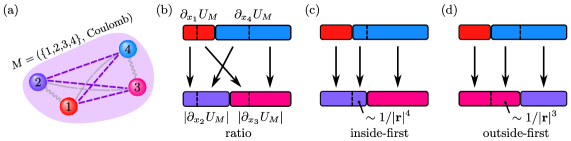
Figure 10: Lifting schemes for a dipole–dipole factor. (a): Dipole–dipole factor with four Coulomb interactions. It is assumed that $\partial_{x_{1}}U_{M}>0$, $\partial_{x_{4}}U_{M}>0$, and $\partial_{x_{2}}U_{M}<0$, $\partial_{x_{3}}U_{M}<0$. (b): “ratio” lifting, (c): “inside-first” lifting (d): “outside-first” lifting.

IV.2 Dipole–dipole lifting schemes

We now consider lifting schemes for dipole–dipole factors, and for concreteness, we consider a four-particle system of particles $\{1,2\}$, forming a charge-neutral dipole $\mathbf{d}_{12}$ and particles $\{3,4\}$, forming an analogous dipole $\mathbf{d}_{34}$. In this two-dipole system, particle $1$, for example, not only interacts with a charge-neutral dipole $\mathbf{d}_{34}$, but is itself inside such a dipole $\mathbf{d}_{12}$. Although the Coulomb lifting rate is oblivious to the position of $2$ (as there is no Coulomb interaction between particles $1$ and $2$), particle $2$ is part of the dipole–dipole factor, and its position influences the relative lifting rates.

We obtain the derivatives with respect to particles $1$ and $2$ for the factor $M=\left(\{1,2,3,4\},\,\text{\text{Coulomb}}\right)$ as follows:

$$\beta\tilde{q}_{M,1}= l_{\text{B}}\left[a\frac{|\mathbf{d}_{34}|}{|\mathbf{r}|^{3}}+\mathcal{O}\left(\frac{|\mathbf{d}_{34}|^{2}}{|\mathbf{r}|^{4}}\right)+\mathcal{O}\left(\frac{|\mathbf{d}_{34}|}{L^{3}}\right)\right],$$ (93)

$$\beta\tilde{q}_{M,2}= l_{\text{B}}\left[-a\frac{|\mathbf{d}_{34}|}{|\mathbf{r}|^{3}}+\mathcal{O}\left(\frac{|\mathbf{d}_{34}|^{2}}{|\mathbf{r}|^{4}}\right)+\mathcal{O}\left(\!\frac{|\mathbf{d}_{34}|}{L^{3}}\!\right)\right].$$ (94)

The dominant terms in these two equations are equal in magnitude yet opposite in sign, reflecting that particles $$1 2 \mathbf{d}_{34} \mathbf{d}_{12} 3 4$$ and interact with the same distant dipole , are of opposite sign, and close to each other (on the dipole ). For the factor derivatives with respect to particles and , we find:

$$\beta\tilde{q}_{M,3}= l_{\text{B}}\left[\tilde{a}\frac{|\mathbf{d}_{12}|}{|\mathbf{r}|^{3}}+\mathcal{O}\left(\frac{|\mathbf{d}_{12}|^{2}}{|\mathbf{r}|^{4}}\right)+\mathcal{O}\left(\frac{|\mathbf{d}_{12}|}{L^{3}}\right)\right],$$ (95)

$$\beta\tilde{q}_{M,4}= l_{\text{B}}\left[-\tilde{a}\frac{|\mathbf{d}_{12}|}{|\mathbf{r}|^{3}}+\mathcal{O}\left(\frac{|\mathbf{d}_{12}|^{2}}{|\mathbf{r}|^{4}}\right)+\mathcal{O}\left(\!\frac{|\mathbf{d}_{12}|}{L^{3}}\!\right)\right].$$ (96)

(For ease of notation, we used here eq. (86) for small $|\mathbf{r}|/L$ rather than the full scaling form.)

The coefficient $a$ (and analogously for $\tilde{a}$) reflects the orientation of $\mathbf{d}_{34}$ with respect to the distance vector between the two dipoles (see Fig. 10). Remarkably, the factor derivatives of $M$ with respect to the particles within each dipole ($\tilde{q}_{M,1}+\tilde{q}_{M,2}$ and $\tilde{q}_{M,2}+\tilde{q}_{M,4}$) cancel at order $1/|\mathbf{r}|^{3}$ and leave a remainder of $1/|\mathbf{r}|^{4}$. This dipole–dipole compensation to order $1/|\mathbf{r}|^{3}$ of the factor derivatives is a general feature for pairs of local dipoles (that can be composed of more than two atoms) inside a factor, and occurs in the same manner with the full scaling functions in the merged-image potential.

Lifting scheme	$q_{\text{intra}}\,\,q_{\text{inter}}$	$\left\langle Q_{\text{intra}}\right\rangle\,\,\,\left\langle Q_{\text{inter}}\right\rangle$	Lifting
particle	$\,0$        $1/|\mathbf{r}|^{2}$	0   $L$	inter-dipole
ratio	$1/|\mathbf{r}|^{3}$  $1/|\mathbf{r}|^{3}$	$\log L\,\,\log L$	inter+intra
outside-first	$1/|\mathbf{r}|^{3}$  $1/|\mathbf{r}|^{3}$	$\log\!\,L\,\,\log\!\,L$	inter+intra
inside-first	$1/|\mathbf{r}|^{3}$  $1/|\mathbf{r}|^{4}$	$\log\!\,L\,\,\,\text{const}$	intra-dipole

Table 1: Coulomb lifting rates for two dipoles separated by a distance $|\mathbf{r}|/L\ll 1$, together with full integrated rate in simulation box of size $L^{3}$: One particle–particle and three dipole–dipole schemes (“ratio”, “outside-first” and “inside-first”). $q_{\text{intra}}$: lifting rate to the non-active particle within the active dipole. $q_{\text{inter}}$: lifting rate to the triggering dipole. $\left\langle Q_{\text{intra}}\right\rangle$ and $\left\langle Q_{\text{inter}}\right\rangle$ denote the mean total event rates (using the full scaling form, as in Section IV.1), integrated over the simulation box.

We recall from eq. (29) that the four factor derivatives exactly sum up to zero. As illustrated in Section II.2 (see Fig. 2), the lifting scheme corresponds to arranging the indices $k^{+}\in I_{M}^{+}$ on the upper row of a two-row table and the indices $k^{-}\in I_{M}^{-}$ on the lower row. In a factor with large separation $|\mathbf{r}|$, each row contains one element corresponding to each of the two dipoles (see Fig. 10).

The “ratio” lifting scheme is as described in Section II.2. All elements fall off as $\mathcal{O}(1/|\mathbf{r}|^{3})$ (see eq. (90)), and both rows contain elements representing each dipole. From eqs (94) and (96), this leads to comparable proportions of intra- and inter-molecular liftings. Both rates fall off at the same rate, but their coefficients are different reflecting the orientations of the dipoles. The total inter- and intra-dipole lifting rates both scale as $\log{L}$ (see Fig. 10b and Table 1).

In the “inside-first” lifting scheme, the elements corresponding to each dipole are aligned with each other. The two match to order $\sim 1/|\mathbf{r}|^{3}$. The mismatch in bar length is $\mathcal{O}(1/|\mathbf{r}|^{4})$ in eqs (93) and (94). In the full scaling picture, the difference in length of the elements can be computed analogously. Coulomb liftings thus occur mostly within a dipole, and long-ranged inter-dipole liftings remain bounded in number for large system sizes (see Fig. 10c and Table 1).

Finally, the “outside-first” lifting scheme consists in vertically aligning elements corresponding to different dipoles. Aligned elements are of length $\sim|a|$ and $\sim|\tilde{a}|$, so that intra- and inter-dipole lifting rates again both fall off as $\mathcal{O}(1/|\mathbf{r}|^{3})$. The situation is analogous to the one for the “ratio” lifting, and the “outside-first” scheme remains strongly non-local (see Fig. 10d and Table 1).

In contrast to the above dipole–dipole factors, the “particle–particle” factor, as argued in eqs (87) and (89), produces events which occur at the scale of the simulation box at a rate which decreases as only $1/|\mathbf{r}|^{2}$, leading to a total event rate increasing linearly with $L$. The lifting flow is between one dipole and the other, and the intra-dipole lifting rate is zero (see Table 1).

IV.3 Validation of factors and liftings

The dipole–dipole factors and their different lifting schemes can be checked for consistency for two charge-neutral dipoles with a short-ranged vibrational intra-dipole potential, a repulsive potential between oppositely charged particles (needed to keep dipoles apart from each other) as well as intermolecular Coulomb interactions. With particles numbered as in Fig. 9, the model corresponds to a factor set

$$\{\left(\{1,2\},\,\text{bond}\right),\left(\{3,4\},\,\text{bond}\right),\left(\{1,4\},\,\text{rep}\right),\\ \left(\{2,3\},\,\text{rep}\right),\left(\{1,2,3,4\},\,\text{Coulomb}\right)\},$$ (97)

with the harmonic bond factor potential,

$$U_{\left(\{i,j\},\,\text{\text{bond}}\right)}(\mathbf{r}_{ij})=\frac{1}{2}k_{b}\left(|\mathbf{r}_{ij}|-r_{0}\right)^{2},$$ (98)

with $k_{b}>0$, a short-range repulsive potential

$$U_{\left(\{i,j\},\,\text{rep}\right)}(\mathbf{r}_{ij})=\frac{1}{2}k_{2}\left(\frac{r_{0}}{|\mathbf{r}_{ij}|}\right)^{6},$$ (99)

with $k_{2}>0$, and a scalar separation $r_{0}$, in addition to the dipole–dipole Coulomb factor potential of eq. (80).

The dipole–dipole Coulomb factor differs from the particle–particle Coulomb factors in the set:

$$\{\left(\{1,2\},\,\text{bond}\right),\left(\{3,4\},\,\text{bond}\right),\left(\{1,4\},\,\text{rep}\right),\\ \left(\{2,3\},\,\text{rep}\right),\left(\{1,3\},\,\text{Coulomb}\right),\left(\{1,4\},\,\text{Coulomb}\right)\\ \left(\{2,3\},\,\text{Coulomb}\right),\left(\{2,4\},\,\text{Coulomb}\right)\},$$ (100)

where the factor potentials corresponding to bond vibrations and the repulsion between unlike charges are as in eqs (98) and (99) and the Coulomb factor potentials are those of eq. (82). In addition, since $|I_{M}|=2$ for each particle-factorized factor $M$, we have no freedom in choosing a lifting scheme (see Section IV.2).

The “ratio”, “inside-first” and “outside-first” lifting schemes for the dipole–dipole factor are easily implemented and compared to the particle–particle lifting scheme. By construction, they yield identical thermodynamic correlations (see Fig. 11). Although the event rates are fixed by the decomposition of the total potential into factors, the different lifting schemes may differ in their dynamical behavior.

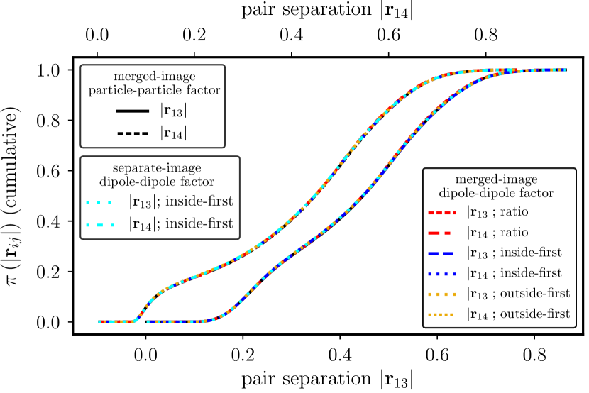
Figure 11: Cumulative histograms of the distances $|\mathbf{r}_{13}|$ (like charges, see Fig. 10a) and $|\mathbf{r}_{14}|$ (opposite charges, see Fig. 10a) for the particle–particle factor set of eq. (100), and also for the factor set of eq. (97) using dipole–dipole Coulomb factors, using the three lifting schemes of Fig. 10b-d. Also separate-image dipole–dipole factors with inside-first lifting. Periodic cubic simulation box with $L=1$, $c_{i}=\pm 1$ point charges, $\beta=1$, $k_{b}=400$, $k_{2}=1$ and $r_{0}=0.1$.

V Liquid water and dipole–dipole factors

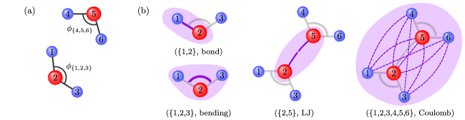
Figure 12: SPC/Fw water model and ECMC factors. (a): Two H₂O molecules, with particles $\{1,2,3\}$ and $\{4,5,6\}$, respectively ($2$ and $5$ being the oxygens). Each of the molecules has a finite dipole moment. (b): “bond”, “bending”, “LJ” and Coulomb factors implementing the SPC/Fw model. Factors contain between two and six particles.

To explore ECMC in a realistic context, we implement in this section the SPC/Fw liquid-water model Wu, Tepper, and Voth (2006). This model combines the long-ranged Coulomb potential with hydrogen–oxygen bond-length vibrations, a flexible hydrogen–oxygen–hydrogen angle, and a specific oxygen–oxygen interaction of the Lennard-Jones type. The SPC/Fw model is closely related to one used in molecular-dynamics simulations of solvated peptides Shaw et al. (2010).

Naturally, each water molecule is charge-neutral and dipolar, so that the dipole–dipole factorization of Section IV applies. This realizes a mean free path for a single particle as $\sim 1/\log\!\,N$ in the thermodynamic limit. (An earlier ECMC Coulomb algorithm Kapfer and Krauth (2016) had obtained a mean-free path of as $\sim 1/N^{1/3}$.)

V.1 Factors in the SPC/Fw water model

To simulate liquid water with the SPC/Fw potential, we use the following type set:

$$\{\,\text{\text{bond}},\,\text{\text{bending}},\,\text{\text{LJ}},\,\text{\text{Coulomb}}\}.$$ (101)

As an example, the factor set for two water molecules, containing particles $\{1,2,3\}$ and $\{4,5,6\}$, respectively, (and with $2$ and $5$ being the oxygens, see Fig. 12a) is:

$$\{\left(\{1,2\},\,\text{\text{bond}}\right),\left(\{2,3\},\,\text{\text{bond}}\right),\\ \left(\{4,5\},\,\text{\text{bond}}\right),\left(\{5,6\},\,\text{\text{bond}}\right),\left(\{2,5\},\,\text{\text{LJ}}\right),\\ \left(\{1,2,3\},\,\text{\text{bending}}\right),\left(\{4,5,6\},\,\text{\text{bending}}\right),\\ \left(\{1,\ldots,6\},\,\text{\text{Coulomb}}\right)\}.$$ (102)

This factor set (see Fig. 12b) trivially generalizes to more than two H₂O molecules.

In eq. (102), the “bond” factor potential of eq. (98) describes oxygen–hydrogen bond vibrations with the equilibrium bond distance $r_{0}=$1.012\text{\,}\mathrm{\SIUnitSymbolAngstrom}$$ and $k_{b}=1059.162\,\mathrm{kcal}\,\mathrm{mol}^{-1}\,\mathrm{rad}^{-2}$, that correspond to the SPC/Fw parameters. The “bending” factor potential describes the fluctuations in the bond angle within each H₂O molecule:

$$U_{\left(\{i,j,k\},\,\text{\text{bending}}\right)}(\mathbf{r}_{i},\mathbf{r}_{j},\mathbf{r}_{k})=\frac{1}{2}k_{a}\left(\phi_{\{i,j,k\}}-\phi_{0}\right)^{2},$$

where $\phi_{\{1,2,3\}}$ and $\phi_{\{4,5,6\}}$ denote the internal angle between the two legs of each H₂O molecule (see Fig. 12). We adopt the SPC/Fw parameters: $\phi_{0}=113.24^{\circ}$ and $k_{a}=75.90\,\mathrm{kcal}\,\mathrm{mol}^{-1}\,{\text{\AA}}^{-2}$. The specific Lennard-Jones interaction between oxygen atoms corresponds to the “LJ” factor potential

$$U_{\left(\{2,5\},\,\text{\text{LJ}}\right)}(\mathbf{r}_{25})=k_{\text{\text{LJ}}}\left[\left(\frac{\sigma}{|\mathbf{r}_{25}|}\right)^{12}-\left(\frac{\sigma}{|\mathbf{r}_{25}|}\right)^{6}\right],$$ (103)

where $k_{\text{\text{LJ}}}=0.62\,\text{kcal}\,\text{mol}^{-1}$ and $\sigma=3.165\,\text{\AA}$ are prescribed in the SPC/Fw model. The Lennard-Jones interaction is truncated beyond $9.0\,\text{\AA}$. Finally, the dipole–dipole “Coulomb” factor potential, in direct generalization of eq. (80), is given by:

$$U_{\left(\{1,\ldots,6\},\,\text{\text{Coulomb}}\right)}(\mathbf{r}_{1},\ldots,\mathbf{r}_{6})\\ =\sum_{i=1}^{3}\sum_{j=4}^{6}U_{\text{C}}(\mathbf{r}_{ij},\{c_{i},c_{j}\}).$$ (104)

Here, the Coulomb potential of eq. (57) is used with the SPC/Fw parameters $c_{1}=c_{3}=c_{4}=c_{6}=0.41e$ and $c_{2}=c_{5}=-0.82e$ (with $e$ the elementary charge).

The type set of eq. (101) is by no means unique. We could also break up the Lennard-Jones interaction into two types, corresponding to the two components of the Lennard-Jones potential (as discussed in Section II.1). Also, instead of the merged-image Coulomb type we could adopt any of the variants of the separate-image type, resulting in a type set:

$$\{\,\text{\text{bond}},\,\text{\text{bending}},\,\text{\text{LJ}},\,\text{\text{Coulomb}}_{\mathbf{n}}:\mathbf{n}\in\mathbb{Z}^{3}\}.$$

Finally, it is possible to break up the “bond” and “bending” factors into $N_{\text{\text{H${}_{2}$O}}}-1$ equal terms in order to construct a unique dipole–dipole factor for each pair of H₂O molecules in such a way that the type set only contains a single element. All these choices are correct, but they may differ in the ease of implementation and in the speed with which they approach equilibrium.

V.2 Intrinsic rotations

Our version of ECMC is formulated in terms of displacements that, for a given event chain, are along one of the directions $\{\hat{\mathbf{e}}_{x},\hat{\mathbf{e}}_{y},\hat{\mathbf{e}}_{z}\}$. Each individual event chain can strain the system, but is unable to rotate it, as the coordinates perpendicular to the direction of motion remain unchanged. The flexible SPC/Fw H₂O molecule may itself get strained in a single event chain. Applying strain subsequently in different directions is known to be equivalent to a rotation on all levels, and in particular on the level of a single molecule. This guarantees that the algorithm is irreducible, and can attain all of configuration space.

The rotation that is induced through subsequent event chains in the three directions can be illustrated in an ECMC simulation of a single H₂O molecule, using only the intramolecular factor types in eq. (101). The rotational dynamics of such a single molecule is easily tracked through the equilibrium autocorrelation function of the dipole moment $\mathbf{d}=\mathbf{r}_{21}+\mathbf{r}_{23}$ (see Fig. 12), given by

$$A(s)=\left\langle\mathbf{d}(s^{\prime})\cdot\mathbf{d}(s^{\prime}+s)\right\rangle\sim\exp\left(-s/\lambda\right)\quad\text{for $s\to\infty$},$$

where the variables $s$ and $s+s^{\prime}$ denote the ECMC displacement (proportional to the time of the continuous Markov process). $A(s)$ decays exponentially at large $s$ with a rate that gives the autocorrelation length $\lambda$ of molecular orientation.

At temperature $300\text{\,}\mathrm{K}$, the cumulative chain length it takes to rotate the molecule around itself is about one to two orders of magnitude larger than the H₂O molecule itself (see Fig. 13). In the limit of large chain lengths $\ell$, the autocorrelation length of the dipole moment is proportional to $\ell$. This simply means that lengthening an already long chain does not add to the internal strain of the water molecule, as a local equilibrium is reached.

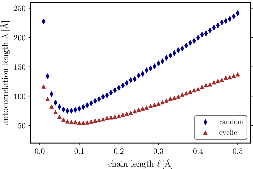
Figure 13: Autocorrelation length $\lambda$ for the dipole moment in ECMC of a single H₂O molecule (fixed chain length $\ell$) for the cyclic sequence of event-chain directions ($\hat{\mathbf{e}}_{x},\hat{\mathbf{e}}_{y},\hat{\mathbf{e}}_{z},\hat{\mathbf{e}}_{x},\dots$) and for their random resampling.

The sequence of chain directions need not be random: The switching of directions merely renders the Markov chain irreducible, whereas global balance is satisfied for any infinitesimal move (without the return move necessary for detailed balance). As a deterministic sequence $\hat{\mathbf{e}}_{x}\hat{\mathbf{e}}_{y}\hat{\mathbf{e}}_{z}\hat{\mathbf{e}}_{x}\hat{\mathbf{e}}_{y}\dots$ avoids repetitions, we find it to decorrelate the dipole moment faster than a uniform random sampling of chain directions (see Fig. 13). The rotations of molecules are thus generated as a byproduct of the switching of event-chain directions. In practical applications, it remains to be seen whether the rotations of molecular ensembles decay particularly slowly. In this case only, the ECMC algorithm will need to be modified in order to explicitly take into account rotations.

V.3 ECMC for liquid water

The SPC/Fw potential is adapted for liquid water at standard temperature $300\text{\,}\mathrm{K}$ and density $1\text{\,}\mathrm{g}\mathrm{/}\mathrm{c}\mathrm{m}^{3}$. An ECMC simulation at these conditions is easily set up with factors (including the dipole–dipole Coulomb factor) as in eq. (102) generalized for $N_{\text{H${}_{2}$O}}>2$. The “ratio”, “outside-first”, and “inside-first” lifting schemes are taken over from the dipole case discussed in Section IV. However, the dipole is now constructed from three particles. For a far distant pair of H₂O molecules, the factor derivatives with respect to the hydrogen positions are usually of the same sign, and of opposite sign to that of the oxygen. In the notations of Fig. 12 and using $M=\left(\{1,\ldots,6\},\,\text{Coulomb}\right)$, we thus have that to order $1/r^{3}$:

$$\partial_{x_{1}}U_{M}\sim\partial_{x_{3}}U_{M}\sim-\frac{1}{2}\partial_{x_{2}}U_{M}.$$ (105)

This can again be used in the inside-first lifting scheme to keep most of the lifting flow inside the molecule of the active particle. Care must be exercised in these lifting schemes to arrange the particles in a fixed order that is independent of which particle is active (it is incorrect to place the active particle systematically on the left-most position on the upper row of the table in Fig. 10).

For long simulation times, the ECMC algorithm exactly samples the Boltzmann distribution of this model, and thermodynamic observables can be compared with Metropolis Monte Carlo using the Ewald summation for the Coulomb potential. This can be verified for the oxygen–oxygen distances that agree to very high precision, demonstrating that the irreversible ECMC converges towards the same steady state as reversible Monte Carlo algorithms (see Fig. 14). To make sure that equilibrium is reached, the initial configurations where chosen randomly in a very dilute system and slowly compressed towards the target density.

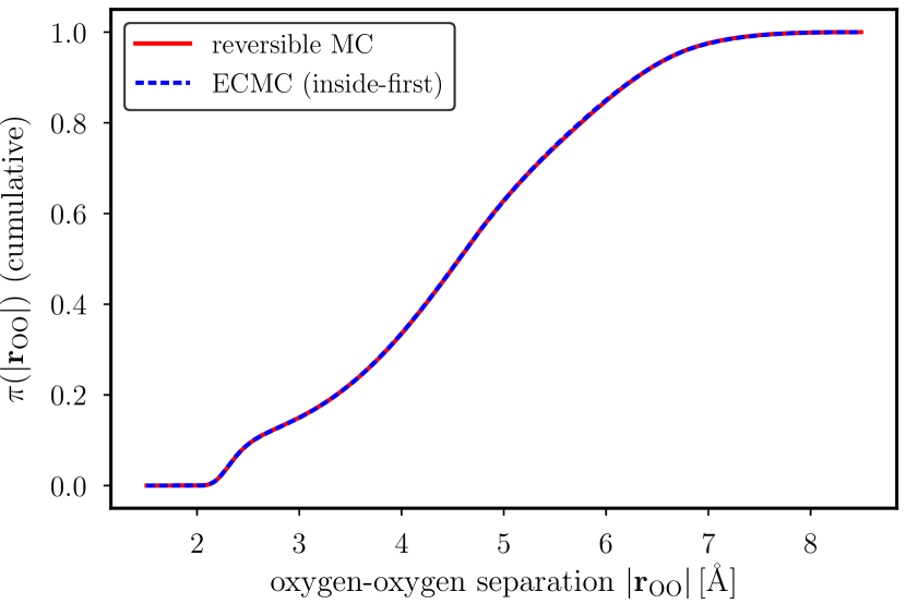
Figure 14: Cumulative histogram of the oxygen–oxygen separation $|\mathbf{r}_{\text{OO}}|$ for $32$ H₂O molecules at standard density and temperature via conventional reversible Monte Carlo and ECMC using the factor set of eq. (102) with inside-first lifting scheme. The random choice of directions was used with a fixed value of $\ell=0.5\text{\AA}$.

In the liquid-water simulation for $N_{\text{H${}_{2}$O}}>2$, the factors $M=\left(I_{M},T_{M}\right)$ belong to four different types (that is, $T_{M}\in\mathcal{T}$ and $|\mathcal{T}|=4$), into which the ensemble-averaged total event rate with respect to particle $k$ (see eq. (21)) can be split:

$$\left\langle Q_{k}(\{\mathbf{r}_{1},\ldots,\mathbf{r}_{N}\})\right\rangle\\ =\sum_{M\in\mathcal{M}}\left\langle q_{M,k}(\{\mathbf{r}_{i}:i\in I_{M}\})\right\rangle=\sum_{T\in\mathcal{T}}\left\langle Q_{T}\right\rangle.$$ (106)

$\left\langle Q_{\text{Coulomb}}\right\rangle$ agrees with the definition in Section III (see eq. (91)). The three local factor types naturally give constant scaling of their associated mean event rates $\left\langle Q_{\text{bond}}\right\rangle$, $\left\langle Q_{\text{LJ}}\right\rangle$, and $\left\langle Q_{\text{bending}}\right\rangle$ with system size, whereas $\left\langle Q_{\text{Coulomb}}\right\rangle$ clearly features $\log N_{\text{H${}_{2}$O}}$ scaling with the number of H₂O molecules (see Fig. 15). The logarithmic scaling of the total Coulomb event rate validates the prediction of eq. (92). The total event rate increases by $$5\text{\,}\mathrm{\SIUnitSymbolAngstrom}$^{-1}$ when $N_{\text{H${}_{2}$O}}$ doubles.

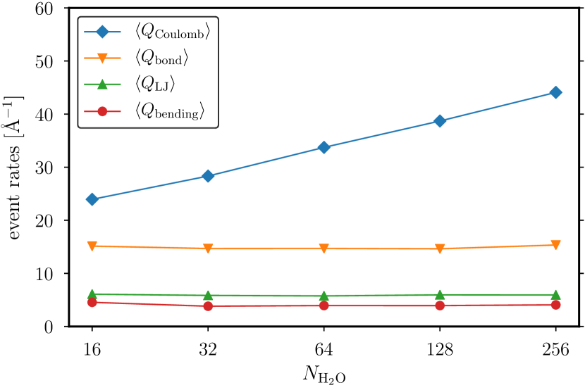
Figure 15: Ensemble-averaged total “Coulomb”, “bond”, “LJ”, and “bending” event rates as a function of the number of H₂O molecules. The Coulomb event rate scales logarithmically. Event rates depend on the choice of factors but are independent of the lifting scheme.

Finally we study the lifting flows for the Couloequ:FactorPotenialWaterBondmb dipole–dipole factors under the “ratio”, “inside-first”, and “outside-first” schemes (see Section IV.2). As discussed in Section IV.1, the event rates are independent of the lifting schemes for a given factor set. However, the probability distributions of the distance $|\mathbf{r}|$ between the active and the target particles are different (see Fig. 16). First, the peak at the oxygen-hydrogen bond length corresponding to a lifting within the molecule increases logarithmically with system size. Second, with increasing system size the distribution of event distances develops a power-law tail. In both the “ratio” and the “outside-first” lifting schemes, the tail of the probability distribution decreases as $|\mathbf{r}|^{-1}$. The “inside-first” scheme decays as $|\mathbf{r}|^{-2}$. These results, corresponding to the evolution of $q_{\text{inter}}$ in $|\mathbf{r}|^{-3}$ and $|\mathbf{r}|^{-4}$ in Table 1.

Remarkably, the “inside-first” lifting scheme induces mostly local lifting flows, even for Coulomb factors that associate H₂O molecules that are far distant from one another. Most of the liftings are local, and the central peak increases as $\log N_{\text{H${}_{2}$O}}$. We expect a local lifting to keep the dynamics of the system coherent, and to lead to faster convergence towards equilibrium. It appears also possible to replace the interaction with far-away H₂O molecules by the interaction with an effective medium (given that the lifting flow remains local). In the “ratio” and “outside-first” lifting schemes, this would probably not be possible as the lifting flow towards far-away dipoles is of the same order of magnitude as the local flow.

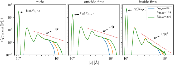
Figure 16: Histogram of distance $|\mathbf{r}|$ between the active and the target particle for the Coulomb events for the “ratio”, “outside-first” and “inside-first” lifting schemes and for 64, 128 and 256 H₂O molecules. The integral of each histogram corresponds to $\left\langle Q_{\text{Coulomb}}\right\rangle$ in Fig. 15. Dashed lines indicate $|\mathbf{r}|^{-z}$ with exponents $z$: $1,1,2$, which corresponds to $q_{\text{inter}}\sim|\mathbf{r}|^{-(z+2)}$ in Table 1.

VI Conclusions

In this work we have outlined the ECMC framework for all-atom computations. Our algorithm advances a single particle in the presence of long-ranged electrostatic interactions in $\mathcal{O}(1)$ operations, with a mean free path which decreases as $\mathcal{O}(1/\log\!\,N)$. This gives an overall complexity of $\mathcal{O}(N\log\!\,N)$ to advance $N$ particles, each by $\mathcal{O}(1)$. This speed can be achieved for locally charge-neutral systems, where particles can be grouped into local dipoles. The algorithm can take into account the presence of free point charges, and its performance worsens only gradually with their number. The algorithm is manifestly translation-invariant and event-driven. It is free of discretization errors, and exactly samples the Boltzmann distribution, without needing a thermostat. Its outstanding property is that it neither computes total forces nor determines the system potential.

ECMC breaks with tradition in two ways. Firstly, as a Markov-chain algorithm, it offers the freedom to choose among a variety of moves. Our approach of advancing single particles may be a first step only. Nevertheless, as we have shown, it effectively rotates dipoles and flexible water molecules in three-dimensional space and samples the entire configuration space. We have explored the great freedom to choose factors and liftings that suit the problem at hand. Secondly, ECMC breaks with tradition in that it is purely Particle–Particle: It treats electrostatic interactions between point charges, but is oblivious to the electrostatic field. This aspect liberates it from the interpolating mesh that in traditional Particle–Particle–Particle–Mesh methods approximates the Coulomb field. Rather, the algorithm is based on the interaction of pairs of particles and, more generally, of factors that may comprise pairs of local dipoles or even more complex objects.

In this work, we have checked that thermodynamic quantities from ECMC agree with those obtained with methods that satisfy detailed balance. As a next step for analyzing ECMC in all-atom systems, it will be important to study its relaxation dynamics in detail. This dynamics will certainly depend on the choice of factors and, for example, for the case of dipole–dipole factors treated here, on the choice of liftings. The inside-first lifting scheme yields mostly local dynamics, and we would expect it to lead to a faster decay of correlation functions. Besides this, we have discussed that the length and the probability distribution of the event-chain parameter $\ell$, and even the sequence of the directions of the event-chain can significantly influence the ECMC dynamics although, as we have verified extensively, the steady state is always given by the Boltzmann distribution. We would hope that, in addition to the overall favorable algorithmic scaling, the fast decay of density fluctuations carries over from short-range-interacting particle and spin systems. The influence of different factorization and lifting schemes on the dynamics of ECMC will also have to be understood. From an algorithmic implementation point of view, we think that the parallelization of the method Kapfer and Krauth (2013) will have to be dealt with carefully.