BELIEF: A distance-based redundancy-proof feature selection method for Big Data.

Abstract

With the advent of Big Data era, data reduction methods are highly demanded given its ability to simplify huge data, and ease complex learning processes. Concretely, algorithms that are able to filter relevant dimensions from a set of millions are of huge importance. Although effective, these techniques suffer from the “scalability” curse as well.

In this work, we propose a distributed feature weighting algorithm, which is able to rank millions of features in parallel using large samples. This method, inspired by the well-known RELIEF algorithm, introduces a novel redundancy elimination measure that provides similar schemes to those based on entropy at a much lower cost. It also allows smooth scale up when more instances are demanded in feature estimations. Empirical tests performed on our method show its estimation ability in manifold huge sets –both in number of features and instances–, as well as its simplified runtime cost (specially, at the redundancy detection step).

1 Introduction

Today the world keeps its relentless pace to the Big Data era by generating quintillion bytes of data daily. We have been surpassed by the challenge of processing such volume of data in a efficient and resilient way. Although researchers are devoting huge effort to cope with voluminous data from the instance side, the opposite side has been largely disregarded by the community despite the more severe implications behind that. Zhai et. al deeply analyzed the dark side of volume in [1]. In this study, authors smartly illustrate the current exponential grow of dimensions in public datasets (millions of features nowadays), as well as the lack of scalability of standard dimensionality reduction (DR) algorithms when facing real-world big data.

Recent developments in technology, science and industry have transformed the explosion of features into reality. Nevertheless, current machine learning (ML) libraries have lagged behind upward trends, thus demanding an urgent revision that enables a rapid learning from large-scale data. Although affected by the same pressing complexity [2], DR techniques are seen as the most certain solution to the curse of dimensionality. They have been widely employed in smaller scenarios to simplify data wideness, and sometimes, have even served to increase subsequent learning performance [3, 4, 5].

From the long taxonomy of DR techniques, the feature selection (FS) family can be highlighted by their high interpretability, popularity, and simplicity [6, 7]. While FS algorithms requires an implicit parameter to delimit the magnitude of selection, feature weighting algorithms offer less constrained schemes based on feature-importance rankings. This subfamily of FS methods is specially relevant for large-scale contexts where interactive selection of thresholds is restricted. Additionally, some of the most outstanding models in FS are focused on feature weighting (e.g.: RELIEF [8]).

Some significant concerns must be addressed by feature selectors in Big Data, specially those based on pairwise correlations as they rapidly shift to trillions when facing millions of features. However, Zhai et al. [1] also underpin the blessing side of the curse showing that in many problems most of features tend to contribute minimally with the correlation objective, and therefore, might be discarded.

Several scalable tools and technologies have emerged in the last years to cope with Big Data. Most of them provide transparent high-level distributed processing services to end-users. MapReduce [9], and its open-source version Hadoop [10, 11], were the pioneer programming models in this area. Recently, a second generation of tools have come along aiming at amending the weaknesses of the first generation. For instance, disk-intensive specialization in Hadoop has being gradually shifted by Apache Spark [12, 13], a framework offering faster memory-based primitives. According to authors, Spark is aimed at accelerating interactive, online, and iterative procedures; normally present in ML algorithms.

Big Data frameworks have given birth to a myriad of large-scale ML libraries, thus enabling standard ML algorithms to perform in huge databases so far unspoiled. MLlib [14], for example, relies on Spark’s operations to speed up the transition between iterations in ML. Although the current state of MLlib is quite advanced, it lacks from several data preprocessing [15] algorithms. Focusing on dimensionality reduction, up to date only the $\chi^{2}$ selector, and an information-theoretic FS framework [16] have been proposed. Still no real scalable feature weighting method has been integrated in Apache Spark up to now (see Section 3.4).

In this work, we propose a distributed design for the feature weighting problem in huge scales inspired by the RELIEF-F algorithm. Our algorithm, called BELIEF, is specially optimized to address large-scale problems with millions of instances and features. Our main contributions with this work are as follows:

• Bridging the gap of dimensionality reduction algorithms in large-scale ML libraries, such as MLlib. In this case, we provide an smart solution for the feature weighting subfield, up to now under-explored.

• Optimization of RELIEF’s main algorithm with two novel procedures: one that squeezes the amount of data transferred during the neighborhood discovery step, and another that replaces instance-wise estimation by one based on the partition scope.

• Built-in redundancy removal to improve selection in problems dominated by feature redundancy. BELIEF takes advantage of feature distances to estimate inter-feature redundancy at nearly zero cost. Our solution based on co-occurrences offers similar schemes to those generated by state-of-the-art information-based measures.

• Comprehensive empirical evaluation of BELIEF. This method has been compared to the current state-of-the-art in distributed FS, showing its advantage in terms of time and precision performance. Datasets with up to $O(10^{7})$ instances and $O(10^{4})$ features have been added to assess the theoretical scalability bounds of our proposal.

The main outline of the paper is as follows. First, some theoretical background information about FS, Big Data, and RELIEF have been captured in Section 2. Then Section 3 describes how BELIEF works, as well as the main optimizations introduced to overcome scalability and redundancy problems. Detailed empirical results and a thorough analysis investigation are embedded in Section 4. Finally, Section 5 outlines the concluding remarks derived from this work.

2 Background

2.1 Feature Selection: problem description and categorization

In data preprocessing, FS algorithms [5] focus on the task of isolating relevant and non-redundant features from the raw set of input features. The pursued objective here is to obtain a simpler and more sanitized subset of features that enables a proper generalization with minimum time cost and predictive degradation. Sometimes output models are not only simpler, but more accurate due to the associated nuances that usually disturb generalization are eliminated [3].

Let $\mathbf{r_{i}}$ be an example $\mathbf{r_{i}}=(r_{i1},\ldots,r_{in},r_{iy})$ from $TR$ (the training set), where $r_{iy}$ value is associated with the output class $y\in C$, whereas $r_{i1}$ value corresponds to the $1$-th feature index, and the $i$-th sample index in the training dataset. $TR$ is formally defined as a bag of $m$ examples, whose instances $\mathbf{r_{i}}$ are formed by a set of input features $X$. Then, the FS problem is trivially defined as the task of finding a subset of features $S_{\theta}\subseteq X$ relevant for the mining process with minimum associated cost.

The current FS state-of-the-art can be roughly summarized in three major categories according to [17]:

1. Wrapper methods: are FS algorithms that rely on a learning method to evaluate fitnesses of features [18]. Wrappers can be deemed as ad-hoc solutions, less prone to perform a proper generalization.

2. Filtering methods: are, on the other hand, independent methods that utilize external measures, such as separability or statistical dependences, to evaluate features. Their generality makes them more appropriate to learn directly from the explicit characteristics of datasets [19].

3. Embedded methods: are integrated methods that exploit a searching procedure implicit in the learning phase [20].

Filtering usually imply a more general/better generalization due to their independence from learners. However, they usually are more conservative at removing features, and require more parameters. Some parameters are crucial for the learning task (e.g.: the number of selected features). They are also more efficient than wrappers, which is advantageous in Big Data environments. This fact explains why most of FS methods implemented in the Big Data literature are based on filtering techniques [15].

2.1.1 Distance-based feature selection

FS methods can alternatively be divided into two groups regarding the shape of output generated: either a subset of features, or a rated list of features (partial or complete) [5]. The latter methods are called rankers, and are one of the most popular subcategory in filtering methods. Rankers rely on a given evaluation measure, such as one based on information dependency or distance, to measure and sort features by predictive importance. Evaluation is performed independently on each feature in these measures. However, although evaluation is performed feature-wisely, it is possible that individual scores somehow imply other features, for example, in redundancy-based measures. Efficient ranking methods are specially relevant for large-scale learning because of its efficiency and simplicity.

Distance measures used in FS range from Euclidean distance to more complex distances like Minkowski distance [21]. Distance measures have not only been bounded to instance-based learning but also applied to class conditional density functions, such as Directed Divergence and Variance. One of the most popular FS solution based on distances is the RELIEF algorithm [22], and its renovated version RELIEF-F [8]. Both are built upon feature distances computed to estimate relevance weights.

RELIEFs are based on the idea that features are deemed relevant as long as they serve to distinguish close instances from alike classes. In RELIEF, we consider a feature $X_{j}\in X$ relevant if for a given instance $\mathbf{r_{i}}$ its near-hit (same class) neighbor $\mathbf{nh}$ is closer than its near-miss (distinct class) neighbor $\mathbf{nm}$ in the space defined by $X_{j}$. Feature-wise distances ($diff$) are accumulated in a weight vector $w$ of size $|X|$ as defined in Equation 1. The parameter $s$ describes the size of the sampling set used in the estimation. The larger $s$, the more reliable is the approximation. This gives us a ranking where we tag as relevant those features whose associated weight exceeds an user-defined relevance threshold $\tau$:

$$w[X_{j}]=w[X_{j}]-diff(nh_{ij},r_{ij})/s+diff(nm_{ij},r_{ij})/s$$ (1)

RELIEF-F [23] extended the original idea of miss-hit by expanding the neighborhood to all classes present in a given multi-class problem (Equation 2). Instead of relying on a single miss, RELIEF-F considers $k$ contributions for each opponent class $NM_{c}$. All contributions are weighted using their respective prior class likelihood as follows:

$$w[X_{j}]=w[X_{j}]-\sum\limits_{i=1}^{k}\frac{diff(nh_{ij},r_{ij})}{s\times k}+\sum_{c\neq y}\sum\limits_{i=1}^{k}\frac{[P(c)\times diff(NM_{cij},r_{ij})]}{s\times k}$$ (2)

Beyond the multi-problem amendment, RELIEF was extended to deal with noise and missing data [23]. Complexity in all RELIEF versions is shared and determined by the neighbor search process, by definition $O(s\times m\times|X|)$.

RELIEF is a reliable estimator whose effectiveness was proven by Kira et al. in [22], among others [24]. Authors showed that under some assumptions the expected weights for relevant features were much larger than those irrelevant. Nevertheless, RELIEF presents some drawbacks like the absence of an explicit mechanism for redundancy elimination. RELIEF directly obviates the final selection set might be fulfilled by both relevant and redundant features, such as those correlated or even duplicated (see Section 2.1.2).

2.1.2 Redundancy elimination in RELIEF models

In recent decades, several variations of RELIEF-F have been proposed. Most of them are focused on providing a solution to the redundancy problem, but there also exist others coping with noise. Here, we outline the most relevant contributions on the redundancy topic, as well as discuss about their possible adaptation to the Big Data environment.

In [25], authors add a posterior phase based on K-means in order to filter out redundancy. K-means discovers cluster of correlated features, and selects those with highest scores as the pivotal elements. Correlation is then the distance measure elected for this algorithm.

Yang et al. [26] proposed the application of Gram-Schmidt orthogonal transformation to detect feature-pair correlations. The idea is to project one of the two feature vectors into the orthogonal dimension, and to re-compute relevance. Authors state that the cosine between the two original features highly influences the new relevance score, and therefore, it determines the correlation between both features. Based on cosine, the algorithm can estimate the redundancy relationship each pair of features.

Conditional RELIEF [27] (CRELIEF) amplifies the original distance-based score idea to one based on three interrelated measures: effectiveness (default), reliability, and informativeness. The latter factor addresses the redundancy problem by relating effectiveness with reliability of higher ranked features. Additionally, authors argue about the necessity of neighbors, and propose to substitute them by random tuples of instances.

Wrapper solutions have also found its niche in the redundancy elimination topic. In [28], Fu et. al proposes to polish RELIEF’s output by applying Support Vector Machine Recursive Feature Elimination as secondary stage. The algorithm starts by dividing the original dataset into several groups in which a single instance of SVM is trained on each one. Feature scores are then normalized and eventually aggregated.

Contrary to the solution above, EN-RELIEF [29] carries out an initial phase of redundancy removal through a regularized linear model. Elastic Net was chosen as the former solution because of its two-norm penalization (L1 and L2). After a post-RELIEF phase, EN-RELIEF generates a sparse vector reflecting the correlation between predictors.

Leaving aside wrappers, all filtering methods described above depends on one way or another on correlation to draw redundancy relationships between features. Notice that the correlation sketch is generated by considering every pair interaction between features which gives us a total of $|X|^{2}$ iterations. In a Big Data context, this is unacceptable as the exponential growth of dimensions is a fact nowadays (see Section 2.2). Consequently, memory and time requirements of current redundancy elimination models should be softened either by reducing the amount of pairwise comparisons, or by alleviating their cost.

2.2 Big Data overview: novel distributed processing tools and techniques and “the curse of dimensionality”

Outstanding technologies, algorithms and tools are required to efficiently process what we call Big Data. The Big Data term was defined by Gartner [30] using the 3Vs concept, namely, high volume, velocity and variety information that require new processing schemes. The V’s list was extended with 2 additional Vs (veracity and value) after a while.

Gartner’s scheme was intended to reflect the increasing number of examples in real-world problems, not envisaging the upcoming phenomenon of Big Dimensionality at least in the first epochs. This phenomenon, also called the “Curse of Dimensionality” [1], revolves around the problem of exponential growth of features and its combinatorial impact in novel datasets.

Little attention have been paid to the curse by ML community despite the exponential growth of dimensions is a fact in most of public data repositories (UCI or libSVM [31, 32]) where it currently measures in the scale of millions.

Despite explosion of correlations sharply affects FS algorithms, Zhai et al. proved in their study [1] FS is in fact an affordable bless for large-scale processing. Studies on the News20 dataset show that features become more sparsely correlated as the dimensionality growths, which imply that the amount of correlation to be accounted is much lower than previously thought. Even so selecting relevant features from the raw set of potentially irrelevant, redundant and noisy features, while complying with the time and storage requirements, is one of the main challenges for scientists and practitioners nowadays.

Big Data processing techniques and tools enable large-scale processing of data within tolerable elapsed times and precision ranges. Google was pioneer in this field by giving birth the MapReduce [9] framework in 2003. MapReduce automatically distributes the load among one or several machines in a easy and transparent way. Unlike other grid computing systems, MapReduce inherently addresses several technical nuances previously controlled by the user. The long list of duties assumed by MapReduce ranges from fault tolerance to network communication, among others.

The final user solely needs to implement two primitives (Map and Reduce) following a key-value scheme. During the Map stage, mappers threads read key-value pairs from local partitions, and transform them into a set of intermediate tuples eventually distributed according to a partitioning scheme (Equation 3). Normally coincident keys are sent to the same node. The Reduce phase read processed pairs and aggregated them to generate a summary result (Equation 4). For extra information about MapReduce and other distributed tools, or the design of distributed algorithms, please refer to [33] and [34].

$$Map(<key_{1},value_{1}>)\rightarrow list(<key_{2},value_{2}>)$$ (3)

$$Reduce(<key_{2},list(value_{2})>)\rightarrow<key_{3},value_{3}>$$ (4)

Despite MapReduce’s popularity in the ML field, the appropriateness of this framework for interactive or iterative processes has been highly criticized [35]. Disk-intensive processing in MapReduce makes it inappropriate or even inapplicable for most of current algorithms.

Apache Spark [36, 13] is a fast and general engine for large-scale data processing designed to overcome the drawbacks presented by Hadoop. Thanks to its built-in memory-based primitives, Spark is able to query data repeatedly deeming it suitable for iterative learning. According to the creators, Spark’s engine is able to run up to 100 times faster than Hadoop in some cases.

Resilient Distributed Dataset (RDD) is the keystone structure on which Spark builds its workflow. RDD operators accompass and extend several distributed models like MapReduce by providing novel and more complex operators. They range from simple filtering and mapping processes to complex joins. As in MapReduce, Spark’s primitives locally transform data within partitions, trying to maintain the data locality property as far as possible. RDDs also allows practitioners to customize data persistence, partitioning and data placement, broadcast read-only variables, track accumulators, and so on. For a full description of Spark operations, see [13].

3 BELIEF: an efficient distributed design for distance-based feature selection

In this section we present BELIEF, a distributed distance-based feature selection algorithm inspired by the popular RELIEF algorithm. BELIEF has been implemented under the Apache Spark development framework to ensure that the two major iterative steps in RELIEF (neighbors searches and weight estimation) are optimized to their fullest degree in the distributed environment.

Neighbor searches are solved in BELIEF by replicating the sample to all the nodes so that distances are completely computed in local (Section 3.1). Neighborhood information for each instance is sent in form of locations to the partitions so that complete instances are not required to be sent. Secondly, BELIEF leverages the previous scheme to create a novel feature weighting estimation procedure where contributions are not instance-wisely anymore, but partition-wise. This mechanism extremely reduces the communication between partitions (Section 3.2).

Besides the time performance enhancements, BELIEF also provides an efficient redundancy removal technique which leverages already computed feature distances to provide redundancy-based weights (Section 3.3).

Algorithm 1 describes BELIEF’s main procedure. It starts by dividing the sample set $S$ into several disjoint batches. Batches are employed in BELIEF for two reasons: to avoid the maximum size allowed by Spark’s broadcasting be surpassed, and to create a feedback procedure between iterations which shorten the list of features to be considered in redundancy calculations. After the split phase, each batch feeds the relevance and redundancy functions. Partial relevance and redundancy matrices are then aggregated and passed to the Sequential Forward Selection (SFS) algorithm which will select features according to Equation 8.

Algorithm 1 BELIEF selection: Main procedure

1:$D$ Dataset

2:$s$ Sample size

3:$b$ # batches

4:$k$ # neighbors

5:$|S|$ # features to be selected

6:$S$ Set of selected features

7:$B\leftarrow$ sample($D,s$).split($b$)

8:$nfeat\leftarrow~{}|X|$

9:$O\leftarrow~{}vector(nfeat)$ $\blacktriangleright$ Marginal likelihood

10:$P\leftarrow~{}matrix(nfeat,nfeat)$ $\blacktriangleright$ Joint likelihood

11:$J\leftarrow~{}vector(nfeat)$ $\blacktriangleright$ Feature weights

12:for $batch~{}\in~{}B$ do

13:   $query\leftarrow~{}$broadcast($batch$)

14:   $NN\leftarrow~{}$broadcast(neighborhood($D,query,k$)) $\blacktriangleright$ Algorithm 2

15:   $J_{p},O_{p},P_{p}\leftarrow~{}$weightEstimation($D,query,NN,k$) $\blacktriangleright$ Algorithm 3

16:   $J\leftarrow J+J_{p};~{}O\leftarrow O+O_{p};~{}P\leftarrow P+P_{p}$

17:end for

18:$I_{\alpha}\leftarrow~{}$computeMCR($O,P$) $\blacktriangleright$ Equation 7

19:$S\leftarrow$ SFS($J,I_{\alpha},|S|$) $\blacktriangleright$ Equation 8

20:return($S$)

3.1 Nearest neighbor search in BELIEF

As we mentioned before, the complexity order of RELIEF, and subsequently BELIEF, is mainly conditioned by the constant seek of neighbors ($\ell=O(s\cdot m)$). Once two examples are paired, weight computations are performed for each feature ($\ell^{*}=O(s\cdot m\cdot\mathbf{|X|})$).

Despite the widely recognized usefulness of RELIEF and other NN-based algorithms, neighbor searches are always compromised by each problem size because of two reasons:

• Execution time: for each search the entire dataset must be revisited. The task is not straightforwardly paralellizable (wide dependencies between partitions). The process becomes even more expensive in case sorting of $k>1$ neighbors is required, which implies to maintain a dedicated structure, such as a bounded heap $O(k\cdot log(k))$.

• Memory consumption: As each pairwise computation must be taken into account in searches, the entire dataset is recommended to be allocated in heap memory. Otherwise, I/O disk operations will dominate global runtime.

The drawbacks mentioned above motivate novel designs for NN search which leverage the distributed technologies presented in Section 2.2, specially those based on in-memory operations.

In this work, we implement distributed searches following the scheme presented in kNN-IS [37]. Assuming $TR$ and $TS$ are split and saved in $p$ disjoint partitions distributed across a cluster of $Z$ nodes. The MapReduce model divides the process into two stages: each mapper reads $p^{*}\leq p$ local partitions from $TR$ and the entire $TS$, computes the distances between each training partition and $TS$. Each reducer collects the local neighbors to each tuple partition-instance and aggregates them by selecting the closest neighbors to them. In our case, $TS$ is replaced by the sampling set in BELIEF.

kNN-IS has proven to be efficient in several real-world problems, however, it presents several bottlenecks to be analyzed. Firstly, the high communication cost derived from the replication of $TS$ to each node (memory consumption: $O(|TS|\cdot|X|$ per node); and secondly, the number of pairs sent to the reducers can become extremely large $p\cdot k\cdot|TS|$, although in this case it is not needed to send the complete instance but only the output variable (classification/prediction) and the distance value. In our case, complexity burden is even worse as $TS$ is replaced by the sampling set in BELIEF. Additionally, BELIEF requires the entire feature vector instead of only the output value.

The reduce step is then revisited in our proposal where entire instances are demanded. However, sending millions of input arrays across the network narrows as invalid, specially in high-dimensional scenarios. The solution adopted consists of sending a lightweight structure that defines the location of candidates in the partitioned dataset. The locator structure is defined as: an integer index pointing at its enclosing partition $I_{g}$, and another index $I_{l}$ for its local position within that partition. This trick reduces the memory and network consumption to $O(|TS|\cdot k\cdot p)$, where $|TS|=s$.

Once candidates are filtered, locators information is broadcasted to every node so that a single map phase can perform BELIEF’s core estimations. Algorithm 2 lists the MapReduce process that describes this process. The following Section explains how the connection between neighbor searches and feature weight estimation.

Algorithm 2 Selection of nearest neighbors for the sample

1:$D$ Dataset

2:$S$ Sample set with size $s$ (broadcasted).

3:$k$ # number of neighbors

4:Neighbors locators $<index,list(<indexP,indexN>)>$

5:   map partitions $<indexP,P>~{}\in~{}D$

6:     for $<index,input>~{}\in~{}S$ do

7:       for $<indexN,inputN>~{}\in~{}P$ do

8:          $d\leftarrow$ computeDistances($inputN$, $input$)

9:          if isTopNN($d$) then

10:             addNN($index$)($indexP,indexN,d$)

11:          end if

12:       end for

13:       emit($<index,addNN(index)>$) $\blacktriangleright$ addNN composed by: $<indexP,indexN,d>$

14:     end for

15:   end map

16:

17:reduce $<index,list(neighbors)>\in D$

18:   $topNN\leftarrow$ selectTopNN(list($neighbors$))

19:   emit($<index,topNN>$) $\blacktriangleright$ topNN composed by pairs: $<indexP,indexN>$

20:end reduce

21:$return(SL)$

3.2 Global weights estimation in BELIEF

The instance-wise estimation model integrated in RELIEF-F have proven to work well in small medical scenarios, such as tumor detection [23] or treatment of myopia [8]. However, its translation to big data scenarios is not straightforward because of the reasons exposed previously. Specifically, sending millions of arrays each time we need to update weights renders as extremely inefficient.

In this paper we propose to re-invent the original RELIEF formula, and to shift from an instance-wise estimation to a more scalable solution based on aggregating partial weights in a partition-wise manner. The pre-conditions we impose for the sake of scalability for this new formulation are:

• For each local process, each sampled instance will have only access to its local neighbors. No communication is allowed between processes. As the entire sample is replicated to all partitions, there will not be degradation in predictive performance.

• Instance-wise output contributions are not longer allowed. A compounding feature-wise solution for each data partition will be the new output.

In order to comply with the previous statements we define a new scheme for distance-based weight estimation, which is indeed applied in a single pass:

$$w[X_{j}]=\sum_{i=1}^{|C|}{\frac{DD_{ij}}{DC_{i}}\times P(C_{i})}-\sum_{i=1}^{|C|}{\frac{ED_{ij}}{EC_{i}}\times P(C_{i})}$$ (5)

where $DD$ and $ED$ are $|C|\times|X|$ matrices that summarize the accumulated feature distance between all sampled instances and its neighbors with distinct and equal class, respectively. $DC$ and $EC$ are $|C|\times 1$ matrices that counts the number of neighbors involved in the calculation of previous $DD$ and $ED$ matrices, respectively.

Matrix computation and weight estimation are computed through two different MapReduce processes described in Algorithm 3. The first phase relies on Equation 2 to compute neighbors’ locations. Then, it creates the feature-class matrices which are updated with distance information. Matrices are eventually aggregated at the subsequent reduce phase. Finally, another MapReduce process (with no reducers) is programmed to apply Equation 5 to each set of matrices.

Algorithm 3 RELIEF’s feature weight estimation

1:$D$ Dataset

2:$S$ Sample set with size $s$ (broadcasted).

3:$NL$ Neighbor locators (broadcasted)

4:Weight by feature

5:   map partitions $<indexP,P>~{}\in~{}D$

6:     $DD\leftarrow$matrix($|C|,|X|$); $ED\leftarrow$matrix($|C|,|X|$)

7:     $DD\leftarrow$matrix($|C|,1$); $EC\leftarrow$matrix($|C|,1$)

8:     for $<index,input,label>~{}\in~{}S$ do

9:       $indices\leftarrow NL$.getLocalLocators($index,indexP$)

10:       for $i~{}\in~{}indices$ do

11:          for $j~{}\in~{}|X|$ do

12:             $distance\leftarrow$ diff($P(i)$.getInput($j$), $input(i)(j)$)

13:             if $P(i)$.label $\neq$ $label$ then

14:               $DD(label)(j)\leftarrow distance$

15:             else

16:               $ED(label)(j)\leftarrow distance$

17:             end if

18:          end for

19:          if $P(i)$.label $\neq$ $label$ then

20:             $DC(label)\leftarrow DC(label)+1$

21:          else

22:             $EC(label)\leftarrow EC(label)+1$

23:          end if

24:       end for

25:     end for

26:     for $j~{}\in~{}|X|$ do

27:       $matrices\leftarrow<DD(*)(j),ED(*)(j),DC(j),EC(j)>$

28:       emit($<j,matrices>$)

29:     end for

30:   end map

31:

32:reduce $<feature,list(matrices)>$

33:   sumMatrices(list($matrices$))

34:end reduce

35:   map $<feature,matrices>~{}$

36:     $weight\leftarrow$ applyBELIEF($matrices$)

37:     emit($<feature,weight>$)

38:   end map

BELIEF’s approach gains scalability and efficiency power with respect to RELIEF, while precision performance remains similar. Although in BELIEF the estimation scope is extended beyond individual instances, our solution keeps unaltered the main idea behind RELIEF. Conceptually the BELIEF method differs from its predecessor in several aspects:

1. In RELIEF each matrix cell would involve an exact $k$ number of neighbors, whereas in BELIEF we resort to standard k-NN search to avoid searches in too broad areas. By weighting each cell value by its neighborhood size this problem is partially addressed.

2. Class likelihood weighting has been extended in BELIEF to the negative part (right side of Equation 5). We understand this model is much more natural and separable for further computations than that presented by RELIEF.

3. As mentioned before, the main improvement introduces revolves around the use of single-pass estimation based on individual feature-class contributions. Though there is substantial shift between both models, BELIEF mimics the same idea based on class separability held in RELIEF. Also notice that some repetitive factors in Equation 1 can be easily removed since they appear in each instance-wise sum, for example, class likelihood or the sample size $s$. In fact, $s$ provides nothing relevant beyond a simple normalization.

3.3 mCR (minimum Collision-based Redundancy): an efficient redundancy removal technique for BELIEF

In Section 2.1.2, we have enumerated different techniques that enable redundancy elimination in RELIEF-F algorithms. Nevertheless, as stated in this section, all these techniques have been designed for small scenarios.

A possible scalable solution for redundancy control may be one based on information theory. An uncertainty measure widely used in the literature is Mutual Information (MI) [38], which expresses the loss of uncertainty of one variable $X_{i}$ after knowing other random variables. MI can be rewritten in entropy terms as follows:

$$I(X_{i};X_{j}) =H(X_{i})-H(X_{i}|X_{j})$$ (6)

$$=\sum_{a\in X_{i}}\sum_{b\in X_{j}}P(a,b)\log\frac{P(a,b)}{P(a)P(b)}.$$

where $X_{i}$ and $X_{j}$ are two discrete random variables with marginal probability mass functions $P(a)$ and $P(b)$, respectively. $H$ represents Shannon entropy, and $P(a,b)$ a joint mass function.

In FS, those features that bears similar information according to MI are considered as redundant, and consequently can be discarded. Some relevant FS filters, like minimum Redundancy Maximum Relevance [39], rely on these information-based measures to make a trade-off with relevancy.

The main drawback of information theoretical techniques is their high complexity. All available combinations between each pair of features (joint likelihood), and all single occurrences in each single feature (marginal likelihood) are accounted for weight estimation, which supposes an unbearable cost in some large-scale scenarios [16].

From the previous formulation we can deduce that entropy is mainly dominated by those co-occurrences more recurrent in the series. Influence of isolated values is then almost negligible. Furthermore, since concrete values in co-occurrences are no longer accounted after being subsumed by the formula, we suggest replacing standard MI by a measure based on directly measuring the number of “collisions” or co-occurrences. This though may imply loss of information and proficiency, it will surely simplifies matrices and computations. After applying Shannon’s entropy to the new “collision” variable, we obtain $I_{\alpha}$:

$$I_{\alpha}(X_{i};X_{j})=PC(X_{i})\log\frac{PC(X_{i},X_{j})}{PC(X_{i})PC(X_{j})}.$$ (7)

where $PC$ represents the likelihood of coincidence within any pair of input feature and/or a single one. We call this measure minimum Collision-based Redundancy (mCR).

mCR can be easily integrated with BELIEF by normalizing both measures and summing their contributions. In our experiments we rely on minmax normalization and a weighting factor $\theta$ to relate both factors. mCR is designed to be integrated in a Sequential Forward Selection process [21] where we start with an empty set of features $S$, and select the best feature in each epoch according to a criteria $J$ until $|S|$ features are selected. Ranks for non-selected features are updated in each iteration taking as reference the last feature selected, and following the formula:

$$J(X_{i})=w(X_{i})-\theta\sum_{X_{j}\in S}I_{\alpha}(X_{j};X_{i}),$$ (8)

where $\theta$ is the factor that weights the impact of redundancy (mCR) and relevance (BELIEF).

One of the most relevant advantages in mCR is that it leverages prior distance values computed in the previous step to construct $PC$ matrices. No extra cost is then associated to mCR beyond the annotation of joint coincidences. Although the number of annotations is infrequent, if this fact is left unmanaged mCR will endure the same problems presented by information-based measures (Section 2.1.2).

In order to control the magnitude of accounted collisions, we introduce a new parameter that limits the number of features considered. The idea is to only update $PC(X_{i},X_{j})$ iff one of them is ranked in top-$(|S|\cdot\eta)$ features by the previous BELIEF phase. It makes sense to leave high irrelevant features aside as they will surely not overtake relevant features in the ranking after the redundancy update. We propose a default value of 2.0 for $\eta$.

mCR is thought to be applied for discrete features where collisions can be easily accounted. However, most of real-world problems partially or entirely consists of continuous features. For continuous scenarios, we propose an alternative solution that replaces 0,1 updates (1 collision hit, 0 otherwise) by a percentage that measures the magnitude of collision, called collision rate $CR$ and defined as follows:

$$CR=1-[(r_{1i}-r_{2i})/\uparrow CR_{X_{i}}]$$ (9)

where $r_{1}$ and $r_{2}$ are two neighbors selected by BELIEF, $\uparrow CR_{X_{i}}$ the maximum collision rate for $X_{i}$ with $\uparrow CR=6\sigma_{i}$ for all the input features, and $\sigma_{i}$ the standard deviation for $X_{i}$.

This decision is motivated by the Chebyshev’s inequality rule which states that 89% of values in most probability distributions are within three standard deviations of the mean. Given that we only focus on the higher collision rates, Chebyshev’s inequality let us to safely ignore outliers, namely, those with the lowest collision values. Another possible solution is to define $\uparrow CR$ equal to the maximum range for each feature, however, this option is highly affected by the shape of distributions.

In order to reduce some effort on annotating coincidences, we establish an upper limit $\kappa$ for collision rates so that values below $\kappa$ are directly skipped. Accepted rates are then utilized to update $PC$ matrices following the scheme $[0\cup[\kappa,1]]$. On the other hand, we apply a Z-score normalization to simplify $\uparrow CR=6\sigma=6$ which improves the homogeneity between features, and at the same time the performance of neighbor searches.

3.4 Other RELIEF adaptations for Big Data tools

In [40], authors proposed a distributed ReliefF-based solution for Apache Spark, called DiReliefF. Despite the algorithm has been successfully tested on real large-scale datasets, authors made some assumptions about the estimation sample which can be deemed as unfair. Namely, they assert that tiny samples with few hundreds of instances are enough to properly estimate class separability in problems formed by millions of instances. As an example, authors states that $6.25\times 10^{-}7\%$ of data in the ECBDL14 problem (see Section 4.1) is enough to correctly underpin feature weights. From our point of view, this premise seems unrealistic as the chance of properly representing millions of instances with such small sample renders as negligible. Experiments focusing on proving the reliability of previous premise will be performed in Section 4.4.

Previous assumptions served as a basement for the optimizations introduced in DiReliefF. For instance, neighborhoods in DiReliefF are computed and moved across the network in their original shape. Although intuitive this procedure impose a high communication cost whenever the number of features or estimation samples increases. Similar cost is imposed by the last step in DiReliefF when neighborhoods are pushed to the driver node to perform feature-side averages. Again this process is simple, but hardly scalable and resource-wasting.

For the above reasons, we think a novel distributed design of ReliefF based on realistic network optimizations, and further enriched with redundancy control techniques can be of great interest for the literature.

4 Empirical evaluation

4.1 Experimental framework

BELIEF has been tested on four large-scale classification datasets, grouped in two categories according to their format and shape. ECBDL14 and epsilon are dense datasets with tabular format, a large number of examples, and a medium number of features. url and kddb are two sparse dataset (from the libSVM repository) formed by millions of key-value pairs.

ECBDL14 is a binary imbalance dataset with an oversampled training set of 65 millions of instances and 631 input features. It is specially remarkable the relevance and difficulty of ECBDL14 given the high imbalance ratio present in the original training set (98%). The remaining datasets are hosted in the LibSVM dataset repository [32]. Their origin, format, and other information can be found in the project’s website.. Table 1 provides basic information about the size and magnitude of all problems.

Table 1: Basic information about the datasets. Included: number of examples for training and test sets (#Train Ex., #Test Ex.), number of features (#Atts.), number of output labels (#Cl) and sparsity condition (binary).

Data Set	#Train Ex.	#Test Ex.	#Atts.	#Cl.	Sparse
epsilon	400 000	100 000	2000	2	No
ECBDL14	65 003 913	2 897 917	630	2	No
url	1 916 904	479 226	3 231 961	2	Yes
kddb	19 264 097	748 401	29 890 095	2	Yes

For comparison purposes we have included a distributed exact version of the minimum Redundancy Maximum Relevance algorithm (DmRMR) [39, 16], implemented in Apache Spark. DmRMR inclusion aims at showing pros and cons of both alternatives, as well as demonstrate the validity of BELIEF. The same argument was proven in [24] where the standard version of both algorithms were compared in a large list of small synthetic datasets.

FS schemes are evaluated using two classification algorithms belonging to the MLlib library [14]: Support Vector Machines (SVM) and Decision Trees (DT). SVMs in Spark internally optimizes the Hinge Loss using Orthant-Wise Limited-memory Quasi-Newton optimizer, whereas DTs perform recursive binary partitioning optimizing an information gain measure (Gini impurity or InfoGain). Parameter configuration for BELIEF is shown in Table 2. Default values for classifiers are left alone. Since all selectors and predictors are based on iterative processes, we cached all the training sets in memory at the beginning.

Table 2: Parameters configuration for selectors

Method	Parameters
BELIEF	k = 3, 5, 10
BELIEF	sampling rate (s) = 0.01, 0.02, 0.25, 0.5
BELIEF	batch size (bs) = 0.1, 0.25
BELIEF	$|S|$ = 10, 50, 100
DmRMR	$|S|$ = 10, 50, 100
BELIEF & DmRMR	Spark partitions = 920

The default level of parallelism was established to 2 times (920) the number of virtual threads available in the cluster (460), thus following the guidelines stated by Spark’s creators .

F1 score (harmonic mean of precision and recall) and prediction accuracy are the two evaluation metrics elected to assess the utility of the selection schemes. To evaluate time performance we rely directly on the overall cluster prediction and feature selection time in seconds.

The cluster involved in the large-scale experiments is composed by 20 slave nodes and 1 master node. The computing nodes hold the following features: 2 CPU processors x Intel Xeon E5-2620, 6 real cores per CPU, 2.00 GHz, 15 MB cache, QDR InfiniBand Network (40 Gbps), 2 TB HDD, 64 GB RAM. All of them running the following software: Apache Spark and MLlib 2.2.0, Hadoop 2.6.0 (HDFS replication factor 2, HDFS default block size 128 MB), 460 virtual threads, 960 RAM GB.

For reproducibility purposes the code have been opensourced and uploaded to GitHub https://github.com/sramirez/spark-RELIEFFC-fselection. In the close future we will send a request for its integration in the main Spark API.

4.2 BELIEF (and mCR) evaluation on small controlled environments

Analysis starts with the evaluation of BELIEF and mCR in small and synthetic problems where relevancy and redundancy is known and well-defined, thus being easier to study algorithms’ behaviors. The same study proposed in a FS review [24] is replicated here in a smaller scale. Table 3 shows the main characteristics of the synthetic datasets used [24], as well as, the composition and nature (relevant/redundant/noise) of synthetic features.

Table 3: Basic information about the synthetic datasets from [24]. From left to right: dataset name, number of rows, number of columns, list of relevant and redundant features, and the baseline accuracy obtained with no FS. (*) SD3 presents six groups of 10 features created to be redundant among themselves; the other 4,000 features are irrelevant. The ideal output is that with one feature from each group.

Dataset	# features	# samples	Relevant	Redundant	Baseline acc.
Corral-100	99	32	1-4	–	56.25%
XOR-100	99	50	1,2	–	52.00%
Parity-3+3	12	64	1-3	4-6	50.00%
SD3	4060	75	G1-G6	*	33.33%
Madelon	500	2400	1-5	6-20	50.13%

Besides accuracy evaluation, we furthermore analyze the composition of the FS schemes generated by using a scoring measure proposed in [24]:

$$Suc.=[\frac{S_{rel}}{X_{rel}}-\zeta\frac{S_{red}}{X_{red}}]\times 100$$ (10)

where $S_{rel},X_{rel}$ is the number of relevant features in $S$ and $X$, respectively. The remaining variables stand for redundant features. The $Suc.$ score described above was designed to penalize redundant features, and to reward relevant selections.

Tables 4 – 8 contains diverse performance information concerning composition, accuracy and success obtained by schemes in mRMR, BELIEF and BELIEF + mCR in five datasets. Specially relevant is the column # red which indicates the degree of redundancy cleaning achieved by each measure. Results shed some light about the potential of the conjunction mCR and BELIEF. This combination overcomes its competitors in 3/5 datasets, being specially relevant in 2/3 datasets with redundant features.

Table 4: Evaluation results for Corral-100. From left to right: the method name, the total number of features selected, and which and how many relevant, redundant and irrelevant are selected. The right-most part contains the prediction results using Naïve Bayes, Decision Tree, and Logistic Regression. Highlighted results in bold indicate the best outcome for each FS scheme.

	Feature Selection						Accuracy
Method	# sel.	Rel.	# rel.	# red.	# irrel.	Success	NB	DT	LR
BELIEF	4	1,3	2	-	2	0.50	0.7105	0.6605	0.6716
	10	1-3	3	-	7	0.75	0.8077	0.6405	0.6216
BELIF+mCR	4	3	1	-	3	0.25	0.6155	0.7266	0.7627
	10	1-3	3	-	7	0.75	0.7466	0.7516	0.7066
mRMR	4	3	1	-	3	0.25	0.6072	0.7266	0.7716
	10	1-4	4	-	6	1.00	0.7655	0.6316	0.8438

Table 5: Evaluation results for XOR-100. From left to right: the method name, the total number of features selected, and which and how many relevant, redundant and irrelevant are selected. The right-most part contains the prediction results using Naïve Bayes, Decision Tree, and Logistic Regression. Highlighted results in bold indicate the best outcome for each FS scheme.

	Feature Selection						Accuracy
Method	# sel.	Rel.	# rel.	# red.	# irrel.	success	NB	DT	LR
BELIF	2	-	0	-	2	0.00	0.7440	1.0000	0.6204
	10	-	0	-	10	0.00	0.7197	0.8383	0.7840
BELIF+mCR	2	-	0	-	2	0.00	0.7440	1.0000	0.6204
	10	-	0	-	10	0.00	0.7190	0.9040	0.6840
mRMR	2	-	0	-	2	0.00	0.4854	0.7157	0.6957
	10	-	0	-	10	0.00	0.7116	0.6173	0.6866

Table 6: Evaluation results for Parity-3+3. From left to right: the method name, the total number of features selected, and which and how many relevant, redundant and irrelevant are selected. The right-most part contains the prediction results using Naïve Bayes, Decision Tree, and Logistic Regression. Highlighted results in bold indicate the best outcome for each FS scheme.

	Feature Selection						Accuracy
Method	# sel.	Rel.	# rel.	# red.	# irrel.	success	NB	DT	LR
BELIEF	3	1,2	2	1	0	0.63	0.3045	0.2902	0.2902
	5	1-3	3	2	0	0.93	0.3045	0.8914	0.2645
BELIEF+mCR	3	1-3	3	0	0	1.00	0.3245	0.8914	0.2645
	5	1-3	3	2	0	0.93	0.3045	0.8914	0.2645
mRMR	3	-	0	0	3	-0.11	0.6195	0.5160	0.6170
	5	2,3	2	0	3	0.56	0.5795	0.4704	0.6295

Table 7: Evaluation results for SD3. From left to right: the method name, the total number of features selected, and which and how many relevant, redundant and irrelevant are selected. The right-most part contains the prediction results using Naïve Bayes, Decision Tree, and Logistic Regression. Highlighted results in bold indicate the best outcome for each FS scheme. Rows with asterisk mean that a previous discretization phase is performed to enable NB prediction.

	Feature Selection					Accuracy
Method	# sel.	# rel.	# red.	# irrel.	success	DT	LR	NB
BELIEF	6	1	5	0	0.17	0.5205	0.5171	-
	20	2	8	10	0.33	0.4927	0.6344	-
BELIEF+mCR	6	1	1	4	0.17	0.5447	0.6033	-
	20	2	7	11	0.33	0.4821	0.7053	-
mRMR	6	2	0	4	0.33	0.8815	0.8758	0.7831
	20	4	3	13	0.67	0.6562	0.9423	0.7921
BELIEF *	6	2	4	0	0.33	0.5780	0.5080	0.1225
	20	3	16	1	0.50	0.7073	0.7058	0.6470
BELIEF+mCR *	6	1	0	5	0.17	0.7240	0.7788	0.6796
	20	4	10	6	0.67	0.6644	0.8006	0.6928

Table 8: Evaluation results for Madelon. From left to right: the method name, the total number of features selected, and which and how many relevant, redundant and irrelevant are selected. The right-most part contains the prediction results using Naïve Bayes, Decision Tree, and Logistic Regression. Highlighted results in bold indicate the best outcome for each FS scheme. Rows with asterisk mean that a previous discretization phase is performed to enable NB prediction.

	Feature Selection						Accuracy
Method	# sel.	Rel.	# rel.	# red.	# irrel.	success	DT	LR	NB
BELIEF	5	-	0	0	5	0.00	0.6890	0.6180	-
	20	-	0	0	20	0.00	0.7664	0.6045	-
BELIEF+mCR	5	-	0	0	5	0.00	0.6890	0.6180	-
	20	-	0	0	20	0.00	0.7953	0.6082	-
mRMR	5	1	1	0	4	0.20	0.6338	0.6083	0.6180
	20	1-5	5	5	10	1.00	0.6742	0.6101	0.6074
BELIEF *	5	-	0	0	5	0.00	0.6337	0.5761	0.5761
	20	1-2	2	0	18	0.40	0.6778	0.6128	0.6195
BELIEF+mCR *	5	-	0	0	5	0.00	0.6337	0.5761	0.5761
	20	1-5	5	0	15	1.00	0.6732	0.6177	0.6058

Furthermore, a pairwise comparison between the two BELIEF alternatives shows a great advantage on using mCR over the standard method. Figure 1 clearly shows this advantage by depicting the difference between the best record achieved by each configuration. In 9/10 records mCR performs better or equal than the standard version. Indeed mCR is not only successful in redundant data ($>50\%$ leap in Parity-3+3), but also effective in redundancy-free problems (e.g.: XOR data).

What it is clear is that mCR perfectly fits its role of redundancy regulator as reflected in Tables 6, 7, and 8. From those tables we can notice the large number of redundant features embraced by standard BELIEF, and how mCR sharply downsizes this set. This fact is also reflected in the success formula, where mCR still performs better.

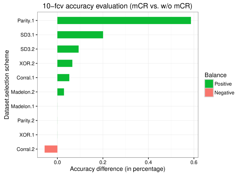
Figure 1: 10-fcv accuracy pairwise comparison BELIEF+mCR vs. BELIEF for several problems and selection schemes. Bars represent the difference between the best marks for each configuration. Row names are composed of the dataset name plus a number (FS configuration, 1: smaller selection, 2: large selection).

4.3 BELIEF evaluation on large environments

Once tested the robustness of mCR in small environments, we move to test its performance in large-scale scenarios. As a starting point, in previous sections we showed how mCR stands as a prominent alternative for small problems. Henceforth we aim at proving that BELIEF stands in large-scale FS as a competitive alternative when compared with the current state-of-the-art.

Starting from a small sampling rate, we provide fine-grained information about the discriminative power of BELIEF in supervised learning. Table 9 shows F1 scores obtained by BELIEF, BELIEF+mCR and DmRMR in 1% sampled. Note that with such small subgroup, BELIEF options are still able to overcome or at least not to be surpassed by DmRMR. Only in kddb, DmRMR is better than BELIEF but with a difference $<1\%$. This fact makes sense as high-dimensional problems have always been a stumble for NN-based algorithms. Conversely, a quantum leap can be noticed in ECBLD14 when applying the tuple BELIEF + mCR.

Table 9: F1-score results after selection and prediction (sampling rate: 0.01, classifier: SVC). In the first column, each block represents a dataset and different parameter configurations for BELIEF. Each of the other columns stand for a single valid FS combination, mixing different thresholds and algorithms. Beliefc indicates BELIEF + mCR. Best score by dataset and threshold is highlighted in bold, the overall best score by dataset is underlined, and the best BELIEF score is marked in italic.

Method/Config.	mRMR	Beliefc	Belief	mRMR	Beliefc	Belief	mRMR	Beliefc	Belief
	100 feat.			50 feat.			10 feat.
epsilon-k5-bs0.25-0	0.7910	0.6597	0.7190	0.7802	0.6175	0.6992	0.6961	0.5973	0.6331
epsilon-k5-bs0.1-0		0.7365	0.7491		0.6909	0.7194		0.6329	0.6647
epsilon-k3-bs0.25-0		0.6445	0.6761		0.6149	0.6487		0.5589	0.3338
epsilon-k3-bs0.1-0		0.6018	0.6625		0.5872	0.6525		0.5135	0.5052
epsilon-k10-bs0.25-0		0.7641	0.7956		0.7247	0.7778		0.6830	0.7050
epsilon-k10-bs0.1-0		0.7320	0.8027		0.7214	0.7910		0.6925	0.7067
baseline-0feat.	0.8976
ecbdl-k5-bs0.25-0	0.4541	0.9749	0.4599	0.4631	0.4729	0.4669	0.5047	0.6650	0.6802
ecbdl-k5-bs0.1-0		0.9749	0.4612		0.4761	0.4694		0.6643	0.6802
ecbdl-k3-bs0.25-0		0.4565	0.4606		0.4885	0.4787		0.6650	0.6803
ecbdl-k3-bs0.1-0		0.9749	0.4606		0.4756	0.4725		0.6651	0.6802
ecbdl-k10-bs0.25-0		0.4521	0.4583		0.4689	0.4709		0.6643	0.6802
ecbdl-k10-bs0.1-0		0.4494	0.4496		0.4675	0.4696		0.6643	0.6643
baseline-0feat.	0.4376
url-k5-bs0.25-0	0.9640	0.9611	0.9605	0.9591	0.9253	0.9263	0.9448	0.9270	0.9269
url-k5-bs0.1-0		0.9608	0.9603		0.9258	0.9393		0.9268	0.9274
url-k3-bs0.25-0		0.9610	0.9598		0.9399	0.9397		0.7016	0.5368
url-k3-bs0.1-0		0.9598	0.9603		0.9412	0.9414		0.5464	0.6869
url-k10-bs0.25-0		0.9605	0.9596		0.9270	0.9274		0.9268	0.9268
url-k10-bs0.1-0		0.9590	0.9600		0.9257	0.9276		0.9268	0.9268
baseline-0feat.	0.9876
kddb-k5-bs0.25-0	0.8413	0.8349	0.8349	0.8093	0.8327	0.8349	0.8349	0.8349	0.8349
kddb-k5-bs0.1-0		0.8343	0.8187		0.8327	0.8327		0.8349	0.8349
kddb-k3-bs0.25-0		0.8187	0.8349		0.8349	0.8327		0.8349	0.8349
kddb-k3-bs0.1-0		0.8349	0.8349		0.8327	0.8155		0.8349	0.8349
kddb-k10-bs0.25-0		0.8187	0.8187		0.8327	0.8349		0.8349	0.8349
kddb-k10-bs0.1-0		0.8349	0.8349		0.8327	0.8327		0.8349	0.8349
baseline-0feat.	?

Focusing on BELIEF versions, we can assert that BELIEF+mCR comes to be more advantageous or similar in $3/4$ datasets. Its poor outcomes in epsilon may be caused by the high noisiness contained in this dataset. Additionally, redundancy among input features in epsilon is negligible.

Table 10 presents similar accuracy results but relying on tree learning to measure predictive power. Outcomes here seem not too illustrative since they tend to reproduce the same behavior shown in Table 9, but with lower scores.

Table 10: F1-score results after selection and prediction phases (sampling rate: 0.01, classifier: DT). In the first column, each block represents a dataset and different parameter configurations for BELIEF. Other columns mean a single combination, mixing different selection thresholds and algorithms. Best score by dataset and threshold is highlighted in bold, overall best score by dataset is underlined, and the best BELIEF score is marked in italic.

Method/Config.	mRMR	Beliefc	Belief	mRMR	Beliefc	Belief	mRMR	Beliefc	Belief-10
	100 feat.			50 feat.			10 feat.
epsilon-k5-bs0.25-0	0.6616	0.6227	0.6516	0.6616	0.6081	0.6516	0.6545	0.6008	0.6269
epsilon-k5-bs0.1-0		0.6550	0.6595		0.6391	0.6595		0.6335	0.6455
epsilon-k3-bs0.25-0		0.6062	0.6386		0.5949	0.6341		0.5591	0.4994
epsilon-k3-bs0.1-0		0.5771	0.6332		0.5769	0.6297		0.5129	0.4982
epsilon-k10-bs0.25-0		0.0000	0.0000		0.0000	0.0000		0.0000	0.0000
epsilon-k10-bs0.1-0		0.0000	0.0000		0.0000	0.0000		0.0000	0.0000
baseline-0feat.	0.6616
ecbdl-k5-bs0.25-0	0.3864	0.4010	0.3481	0.3864	0.3994	0.3373	0.3225	0.4374	0.4732
ecbdl-k5-bs0.1-0		0.3577	0.4209		0.4328	0.4136		0.4366	0.4716
ecbdl-k3-bs0.25-0		0.3609	0.3511		0.4798	0.3373		0.4374	0.4779
ecbdl-k3-bs0.1-0		0.3978	0.3478		0.4327	0.3355		0.4373	0.4729
ecbdl-k10-bs0.25-0		0.4379	0.3608		0.4368	0.3566		0.4368	0.4716
ecbdl-k10-bs0.1-0		0.3800	0.4070		0.3458	0.4178		0.4388	0.4388
baseline-0feat.	0.3789
url-k5-bs0.25-0	0.9635	0.9573	0.9573	0.9586	0.9587	0.9424	0.9568	0.9375	0.9375
url-k5-bs0.1-0		0.9574	0.9574		0.9586	0.9425		0.9375	0.9375
url-k3-bs0.25-0		0.9573	0.9573		0.9490	0.9490		0.7671	0.8075
url-k3-bs0.1-0		0.9577	0.9577		0.9490	0.9490		0.8073	0.8055
url-k10-bs0.25-0		0.9573	0.9573		0.9428	0.9457		0.9375	0.9373
url-k10-bs0.1-0		0.9577	0.9577		0.9608	0.9425		0.9395	0.9395
baseline-0feat.	?
kddb-k5-bs0.25-0	0.8376	0.8349	0.8349	0.8372	0.8349	0.8349	0.8367	0.8349	0.8349
kddb-k5-bs0.1-0		0.8349	0.8349		0.8349	0.8349		0.8349	0.8349
kddb-k3-bs0.25-0		0.8349	0.8349		0.8349	0.8349		0.8349	0.8349
kddb-k3-bs0.1-0		0.8349	0.8349		0.8349	0.8349		0.8349	0.8349
kddb-k10-bs0.25-0		0.8349	0.8349		0.8349	0.8349		0.8349	0.8349
kddb-k10-bs0.1-0		0.8349	0.8349		0.8349	0.8349		0.8349	0.8349
baseline-0feat.	?

4.4 Sampling rate impact on BELIEF

In this section we inspect precision and runtime performance as sampling rate augments, as well as, to analyze the possible negative impact of an excessively small rate. Figures 2 and 3 contain information about the impact of sampling size on accuracy (F1-score). In Figure 2, we can observe the stability of scores as sampling augments. According to the graph, only $1\%$ of data is enough to properly estimate weights in most of cases (except in epsilon). Time measurements recorded in Figure 3 also confirm low rates in BELIEF provides lower reaction times compared to DmRMR.

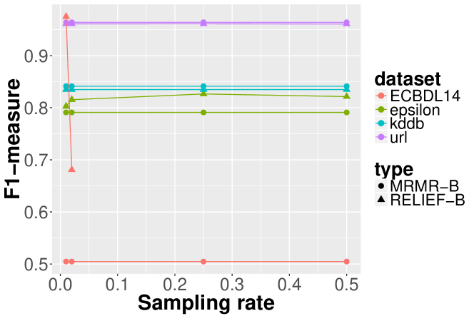
Figure 2: Evolution of F1 measure as sampling rate is increased. For each dataset the most accurate record is depicted. MRMR-B stands for DmRMR with 100 features selected.

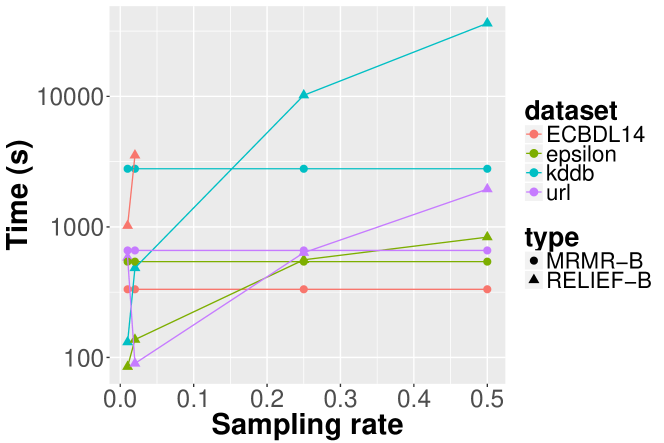
Figure 3: Evolution of runtime performance as sampling rate is increased. For each dataset the most accurate record is depicted. MRMR-B stands for DmRMR with 100 features selected.

In case we rather focus on rapid solutions, Figures 4 and 5 depict empirical results for the most agile configurations in BELIEF and DmRMR. According to these results, we can underpin BELIEF again as the most effective and efficient alternative for low-rate scenarios. For 1% sampled data, BELIEF obtains substantial benefits with respect to DmRMR regarding time performance. Beyond a higher accuracy, low-rate solutions plus offer faster response times than DmRMR. Higher rates seems to be not interesting because of their high runtime cost and lack of accuracy improvement.

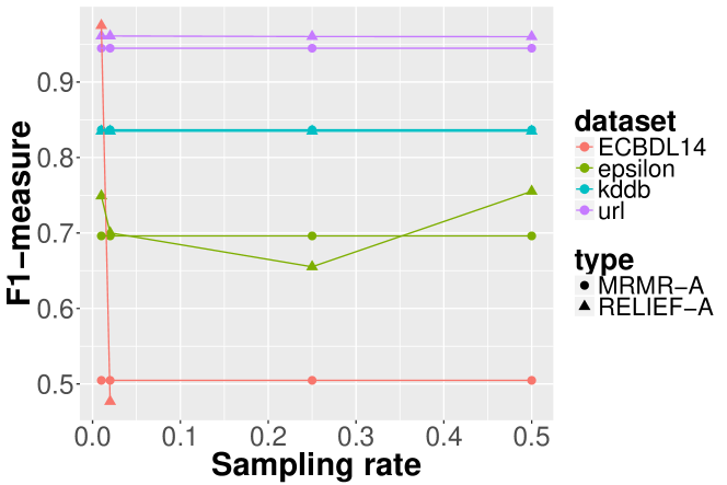
Figure 4: Evolution of F1 measure as sampling rate is increased. For each dataset the most rapid record is depicted. MRMR-A stands for DmRMR with 10 features selected.

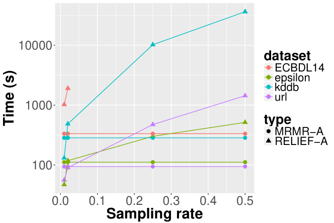
Figure 5: Evolution of runtime performance as sampling rate is increased. For each dataset the most rapid record is depicted. MRMR-A stands for DmRMR with 10 features selected.

In order to study the impact of sampling over-reduction on feature weighting, we have compared the precision results obtained by our smallest scheme (1% of sampling) against those proposed in DiReliefF [40], with only 100 instances. Results on both datasets show a clear drop on F1 score when using extremely small rates, such as only 100 instances from datasets with millions. Then, we can assert with some certainty proper sampling rates render as essential to obtain fair estimations. A solution that allows scaling of sampling set is thus required.

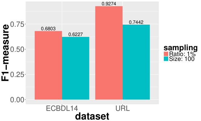
Figure 6: Impact on F1 score associated to over-reduction on sampling rate: 100 instances sampled vs. 1% of sampling rate (about thousands). One dataset for each type was selected (sparse and dense). And the selection number was bounded to the most demanding configuration, namely, only 10 features.

5 Concluding Remarks

In this paper, we have presented BELIEF, a feature weighting algorithm capable of accurately estimating feature importance in large samples –both in number of features and examples–. With this new proposal we aimed at solving the performance deficiencies shown by RELIEF and its distributed versions when facing big datasets, concretely, large estimation samples. By restricting network communication among partitions, and the scope of main computations (moving from instance-wise to partition-wise) in RELIEF, we have managed to create a proper distributed version able to naturally scale up as requested.

Aside from the fully-scalable model, we have addressed lack of redundancy management techniques in RELIEF models by proposing a built-in redundancy removal procedure that detects and eliminates duplicities in selections. Our solution (mCR) relies on feature co-occurrences (collisions) already computed to estimate strong dependencies among input features at barely no time cost. Experiments performed on small data confirmed that no substantial difference between schemes generated by mCR and other information-based models exists beyond a higher cost imposed by the latter ones.

Extended tests comprising several real-world datasets –up to $O(10^{7})$ instances and $O(10^{4})$ features– have asserted as well the relevance of BELIEF in large environments. Results shed light about BELIEF’s predominance in terms of runtime performance and precision of schemes when compared to alternative models such as DiReliefF. As future work, we plan to incorporate some mechanisms to further expedite neighbor searches in BELIEF. They will be based on locality sensitivity hashing tables, or metric trees.

References

- [1] Y. Zhai, Y. Ong, I. W. Tsang, The emerging “big dimensionality”, IEEE Computational Intelligence Magazine 9 (3) (2014) 14–26.
- [2] V. Bolón-Canedo, N. Sánchez-Marono, A. Alonso-Betanzos, Recent advances and emerging challenges of feature selection in the context of big data, Knowledge-Based Systems 86 (2015) 33 – 45.
- [3] I. Guyon, S. Gunn, M. Nikravesh, L. A. Zadeh, Feature Extraction: Foundations and Applications (Studies in Fuzziness and Soft Computing), 2006.
- [4] Z. Zhao, H. Liu, Spectral feature selection for data mining, Chapman & Hall/CRC, 2011.
- [5] V. Bolón-Canedo, N. Sánchez-Maroño, A. Alonso-Betanzos, Feature Selection for High-Dimensional Data, Artificial Intelligence: Foundations, Theory, and Algorithms, Springer, 2015.
- [6] Q. Wu, Z. Wang, F. Deng, Z. Chi, D. Feng, Realistic human action recognition with multimodal feature selection and fusion, Systems, Man, and Cybernetics: Systems, IEEE Transactions on 43 (4) (2013) 875–885.
- [7] V. Bolón-Canedo, N. S.-M. no, A. Alonso-Betanzos, J. Benítez, F. Herrera, A review of microarray datasets and applied feature selection methods, Information Sciences 282 (2014) 111 – 135.
- [8] I. Kononenko, E. Šimec, M. Robnik-Šikonja, Overcoming the myopia of inductive learning algorithms with RELIEFF, Applied Intelligence 7 (1) (1997) 39–55.
- [9] J. Dean, S. Ghemawat, MapReduce: Simplified data processing on large clusters, in: Proceedings of the 6th Conference on Symposium on Opearting Systems Design & Implementation, Vol. 6 of OSDI’04, 2004, pp. 10–10.
- [10] T. White, Hadoop, The Definitive Guide, O’Reilly Media, Inc., 2012.
-
[11]
Apache Hadoop Project, Apache Hadoop,
[Online; accessed May 2018] (2018).
URL http://hadoop.apache.org/ - [12] M. Zaharia, M. Chowdhury, T. Das, A. Dave, J. Ma, M. McCauley, M. J. Franklin, S. Shenker, I. Stoica, Resilient distributed datasets: A fault-tolerant abstraction for in-memory cluster computing, in: Proceedings of the 9th USENIX Conference on Networked Systems Design and Implementation, NSDI’12, 2012, pp. 2–2.
-
[13]
Apache Spark: Lightning-fast cluster computing,
Apache spark, [Online; accessed May 2018]
(2018).
URL https://spark.apache.org/ - [14] X. Meng, J. Bradley, B. Yavuz, E. Sparks, S. Venkataraman, D. Liu, J. Freeman, D. Tsai, M. Amde, S. Owen, D. Xin, R. Xin, M. J. Franklin, R. Zadeh, M. Zaharia, A. Talwalkar, Mllib: Machine learning in apache spark, Journal of Machine Learning Research 17 (34) (2016) 1–7.
- [15] S. García, S. Ramírez-Gallego, J. Luengo, J. M. Benítez, F. Herrera, Big data preprocessing: methods and prospects, Big Data Analytics 1 (1) (2016) 9.
- [16] S. Ramírez-Gallego, H. M. no Talín, D. Martínez-Rego, V. Bolón-Canedo, J. M. Benítez, A. Alonso-Betanzos, F. Herrera, An information theory-based feature selection framework for big data under apache spark, IEEE Transactions on Systems, Man, and Cybernetics: Systems (2017) 1–13.
- [17] A. L. Blum, P. Langley, Selection of relevant features and examples in machine learning, Artificial Intelligence 97 (1-2) (1997) 245–271.
- [18] R. Kohavi, G. H. John, Wrappers for feature subset selection, Artificial Intelligence 97 (1-2) (1997) 273–324.
- [19] I. Guyon, A. Elisseeff, An introduction to variable and feature selection, Journal of Machine Learning Research 3 (2003) 1157–1182.
- [20] Y. Saeys, I. n. Inza, P. Larrañaga, A review of feature selection techniques in bioinformatics, Bioinformatics 23 (19) (2007) 2507–2517.
- [21] S. García, J. Luengo, F. Herrera, Data Preprocessing in Data Mining, Springer, 2015.
- [22] K. Kira, L. A. Rendell, A practical approach to feature selection, in: Proceedings of the Ninth International Workshop on Machine Learning, ML92, Morgan Kaufmann Publishers Inc., 1992, pp. 249–256.
- [23] I. Kononenko, Estimating attributes: Analysis and extensions of relief, Springer Verlag, 1994, pp. 171–182.
- [24] V. Bolón-Canedo, N. Sánchez-Maroño, A. Alonso-Betanzos, A review of feature selection methods on synthetic data, Knowledge and information systems 34 (3) (2013) 483–519.
- [25] J. Bins, B. A. Draper, Feature selection from huge feature sets, in: Proceedings Eighth IEEE International Conference on Computer Vision. ICCV 2001, Vol. 2, 2001, pp. 159–165.
- [26] J. Yang, Y.-P. Li, Orthogonal relief algorithm for feature selection, in: Proceedings of the 2006 International Conference on Intelligent Computing - Volume Part I, ICIC’06, 2006, pp. 227–234.
- [27] T. Wu, K. Xie, C. Nie, G. Song, An adaption of relief for redundant feature elimination, in: Advances in Neural Networks - ISNN 2012 - 9th International Symposium on Neural Networks, Shenyang, China, July 11-14, 2012. Proceedings, Part II, 2012, pp. 73–81.
- [28] R. Fu, P. Wang, Y. Gao, X. Hua, A new feature selection method based on relief and svm-rfe, in: 12th International Conference on Signal Processing (ICSP), 2014, pp. 1363–1366.
- [29] N. Challita, M. Khalil, P. Beauseroy, New technique for feature selection: Combination between elastic net and relief, in: Third International Conference on Technological Advances in Electrical, Electronics and Computer Engineering (TAEECE), 2015, pp. 262–267.
-
[30]
M. Beyer, D. Laney,
3d
data management: Controlling data volume, velocity and variety (2001).
URL http://blogs.gartner.com/doug-laney/files/2012/01/ad949-3D-Data-Management-Controlling-Data-Volume-Velocity-and-Variety.pdf -
[31]
K. Bache, M. Lichman, UCI machine
learning repository (2013).
URL http://archive.ics.uci.edu/ml - [32] C.-C. Chang, C.-J. Lin, LIBSVM: A library for support vector machines, ACM Transactions on Intelligent Systems and Technology 2 (2011) 27:1–27:27, datasets available at http://www.csie.ntu.edu.tw/~cjlin/libsvmtools/datasets/.
- [33] A. Fernández, S. del Río, V. López, A. Bawakid, M. J. del Jesús, J. M. Benítez, F. Herrera, Big data with cloud computing: an insight on the computing environment, mapreduce, and programming frameworks, Wiley Interdisciplinary Rewiews: Data Mining and Knowledge Discovery 4 (5) (2014) 380–409.
- [34] S. Ramírez-Gallego, A. Fernandez, S. García, M. Chen, F. Herrera, Big Data: Tutorial and guidelines on information and process fusion for analytics algorithms with mapreduce, Information Fusion 42 (2018) 51–61.
- [35] J. Lin, Mapreduce is good enough? if all you have is a hammer, throw away everything that’s not a nail!, Big Data 1 (1) (2013) 28–37.
- [36] M. Hamstra, H. Karau, M. Zaharia, A. Konwinski, P. Wendell, Learning Spark: Lightning-Fast Big Data Analytics, O’Reilly Media, Incorporated, 2015.
- [37] J. Maillo, S. Ramírez, I. Triguero, F. Herrera, kNN-IS: An iterative spark-based design of the k-nearest neighbors classifier for big data, Knowledge-Based Systems 117 (Supplement C) (2017) 3 – 15, volume, Variety and Velocity in Data Science.
- [38] T. M. Cover, J. A. Thomas, Elements of Information Theory, 1991.
- [39] H. Peng, F. Long, C. Ding, Feature selection based on mutual information criteria of max-dependency, max-relevance, and min-redundancy, Pattern Analysis and Machine Intelligence, IEEE Transactions on 27 (8) (2005) 1226–1238.
- [40] R.-J. Palma-Mendoza, D. Rodriguez, L. de Marcos, Distributed ReliefF-based feature selection in Spark, Knowledge and Information Systems, in press. doi:10.1007/s10115-017-1145-y.