Ultrafast destruction and recovery of the spin density wave order in iron based pnictides: a multi-pulse optical study

?abstractname?

We report on systematic excitation-density dependent all-optical femtosecond time resolved study of the spin-density wave state in iron-based superconductors. The destruction and recovery dynamics are measured by means of the standard and a multi-pulse pump-probe technique. The experimental data are analyzed and interpreted in the framework of an extended three temperature model. The analysis suggests that the optical-phonons energy-relaxation plays an important role in the recovery of almost exclusively electronically driven spin density wave order.

I Introduction

The collectively ordered electronic states are interesting subjects for driving out of equilibrium by femtosecond optical pulses in order to get better insight into their natureIwai et al. (2007); Kübler et al. (2007); Schmitt et al. (2008); Tomeljak et al. (2009); Petersen et al. (2011); Schmitt et al. (2011); Beaud et al. (2014); Smallwood et al. (2014); Madan et al. (2016) and possibly reveal new meta-stable statesIchikawa et al. (2011); Stojchevska et al. (2014); Morrison et al. (2014) that are not easily reachable by the quasi-equilibrium route. Among such states is also the orthorhombic antiferromagnetic spin-density-wave like state in the parent iron-based superconductors compoundsKamihara et al. (2006, 2008); Stewart (2011), which is interesting not only due to the proximity to the superconducting state but also due to its collective itinerant nature and relation to the nematicChuang et al. (2010); Chu et al. (2010); Dusza, A. et al. (2011) instability.

The ultrafast dynamics of the spin density wave (SDW) state in pnictides has been extensively studied by various time resolved techniquesMertelj et al. (2010); Stojchevska et al. (2010); Rettig et al. (2012); Kim et al. (2012); Pogrebna et al. (2014); Patz et al. (2014); Gerber et al. (2015); Rettig et al. (2016). All-opticalPogrebna et al. (2014) and time resolved (TR) ARPESRettig et al. (2012) studies show sub-picosecond dynamics with slight slowing down near the transition temperature, while the orthorhombic lattice splitting responds much slowerGerber et al. (2015); Rettig et al. (2016) upon the ultrafast perturbation. An interesting question is what sets the sub-picosecond timescale of the suppression and recovery of the electronic SDW order? At weak suppression it appears that the timescale is set by the bottleneck in the relaxation of the nonequilibrium electron distribution function (NEDF) due to the charge gap associated with the SDW order.Stojchevska et al. (2010); Pogrebna et al. (2014) At strong suppression the charge-gap bottleneck is suppressed an the collective SDW dynamics and/or the electron phonon coupling might play a role in setting the timescale.

In order to improve understanding of the suppression and recovery timescales at strong suppression we conducted a systematic fluence-dependent femtosecond time-resolved all-optical study of the SDW state in two iron-based superconductors parent compounds: AFe₂As₂ (A=Eu,Sr). In the study we supplemented the standard pump-probe technique with the multipulse technique that proved to be instrumentalYusupov et al. (2010); Madan et al. (2016) to obtain insights into the collective dynamics in charge density wave systemsYusupov et al. (2010) and superconductorsMadan et al. (2016).

To identify the processes that set the SDW recovery time we analyze the multipulse data in the framework of an extended three temperature model (3TM). Surprisingly, the 3TM analysis suggests that an excitation density dependent optical-phonons - lattice-bath energy-relaxation bottleneck plays a crucial role in the the NEDF relaxation and the SDW order recovery while the collective SDW order dynamics is too fast to influence the dynamics beyond $\sim 200$ fs. Moreover, the resilience of the SDW state to strong ultrafast optical excitation is suggested to be a consequence of a fast electron - optical-phonon energy transfer during the initial NEDF thermalization on a few hundred femtosecond timescale that is enhanced at high excitation densities.

II Experimental

II.1 Samples

Single crystals of EuFe₂As₂ (Eu-122) and SrFe₂As₂ (Sr-122) were grown at Zhejiang University by a flux method as described previously.Pogrebna et al. (2014) In both compounds the onset of the antiferromagnetic SDW-like ordering is concurrent with the structural transition from tetragonal to orthorhombic symmetry $T_{\mathrm{N}}=190$ K for Eu-122Tegel et al. (2008) and $T_{\mathrm{N}}=203$ K for Sr-122.Tegel et al. (2008)

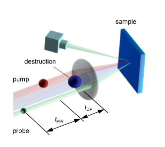
?figurename? 1: (Color online) Schematic representation of the three-pulse experiment and notation of the delays between pulses.

II.2 Optical setup

Measurements of the multi-pulse transient reflectivity were performed using an extension of the standard pump-probe technique, with $\sim 50$ fs optical pulses from either 1-kHz or 250-kHz Ti:Al₂O₃ regenerative amplifiers seeded with Ti:Al₂O₃ oscillators. The output pulse train was split into destruction (D), pump (P) and probe (Pr) pulse trains that were independently delayed with respect to each other. The P and D pulse beams were either at the laser fundamental ($\hbar\omega_{\mathrm{P}}=1.55$ eV) or the doubled ($\hbar\omega_{\mathrm{P}}=3.1$ eV) photon energy, while the Pr beam was always at the the laser fundamental $\hbar\omega_{\mathrm{pr}}=1.55$ eV photon energy.

The resulting beams were focused and overlapped on the sample (see Fig. 1). As in the standard pump-probe stroboscopic experiments the multipulse transient reflectivity $\Delta R_{3}/R$ was measured by monitoring the intensity of the weakest Pr beam. The direct contribution of the unchopped D beam to the total transient reflectivity, $\Delta R$, was rejected by means of a lock-in synchronized to the chopper that modulated the intensity of the P beam only. The fluences of the P and Pr pulses, $\mathcal{\mathcal{F_{\mathrm{Pr}}}<F_{\mathrm{P}}}\lesssim 100$ $\mu$J/cm², were kept in the linear response region.

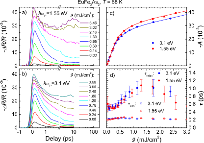
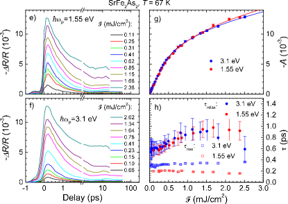
?figurename? 2: (Color online) Fluence dependence of the transient reflectivity in the SDW state for the $\mathcal{P}^{-}$ probe polarization in Eu-122 (a), (b) and Sr-122 (e), (f) at two different pump-photon energies. The amplitude of the transient reflectivity as a function of the pump fluence in Eu-122 (c) and Sr-122 (g). The corresponding transient reflectivity decay and rise times as a function of the pump fluence are shown in (d) and (h). The thin lines in (c) and (g) are the saturation model fits discussed in text.

Due to the chopping scheme the measured quantity in the multipulse experiments is the difference between the transient reflectivity in the presence of P and D pulses, $\Delta R_{\mathrm{DP}}(t_{\mathrm{Pr}},t_{\mathrm{P}},t_{\mathrm{D}})$, and the transient reflectivity in the presence of the D pulse only, $\Delta R_{\mathrm{D}}(t_{\mathrm{Pr}},t_{\mathrm{D}})$:

$$\Delta R_{3}(t_{\mathrm{Pr}},t_{\mathrm{P}},t_{\mathrm{D}})=\Delta R_{\mathrm{DP}}(t_{\mathrm{Pr}},t_{\mathrm{P}},t_{\mathrm{D}})-\Delta R_{\mathrm{D}}(t_{\mathrm{Pr}},t_{\mathrm{D}}),$$ (1)

where $t_{\mathrm{Pr}}$, $t_{\mathrm{P}}$ and $t_{\mathrm{D}}$ correspond to the Pr, P and D pulse arrival times, respectively.

When using the doubled P-photon energy the scattered pump photons were rejected by long-pass filtering, while an analyzer oriented perpendicularly to the P-beam polarization was used for rejection in the case of the degenerate P- and Pr-photon energies. All beams were nearly perpendicular to the cleaved sample surface (001). Both, the P and D beam had polarizations perpendicular to the polarization of the Pr beam, which was oriented with respect to the crystals to obtain the maximum or minimum amplitude of the sub-picosecond $\Delta R/R$ at low temperatures. The pump beam diameters were, depending on experimental conditions, in a 50-100 $\mu$m range with somewhat smaller probe beam diameters. The beam diameters were determined either by a direct measurement of the profile at the sample position by means of a CMOS camera or by measuring the transmission through a set of calibrated pinholes.

III Standard pump-probe results

As noted previouslyPogrebna et al. (2016) we observe a 2-fold rotational anisotropy of the transient reflectivity with respect to the probe polarization with different orientation in different domains. To measure a single domain dominated response the positions on the sample surface with maximal anisotropy of the response have been chosen for measurements. In the absence of information about the in-plane crystal axes orientation in the chosen domains we denote the probe-polarization orientation according to the polarity of the observed sub-picosecond low-$T$ response as $\mathcal{P}^{+}$ and $\mathcal{P}^{-}$. The magnitude of the $\mathcal{P}^{-}$ response is larger than the magnitude of the $\mathcal{P}^{+}$ response in both compounds so in the multi-pulse experiments the $\mathcal{P}^{-}$ Pr polarization was used in most of the cases.

III.1 Fluence dependence

In Fig. 2 we plot the fluence dependence of the standard 2-pulse transient reflectivity in the SDW state. In both compounds we observe a linear scaling of $\Delta R/R$ with the pump fluence ($\mathcal{F}_{\mathrm{P}}$) up to the threshold fluence, $\mathcal{F}_{\mathrm{th}}\sim 0.2$ mJ/cm². Above this value the amplitude of the initial sub-ps transient shows a partial saturation increasing linearly with a different slope and nonzero intercept above $\mathcal{F}_{\mathrm{P}}\sim 1$ mJ/cm². In this region of fluence also a long lived component following the initial sub-ps transient becomes rather prominent.

The risetime of the transients, $\tau_{\mathrm{rise}}$, shows no fluence dependence while the initial sub-ps decay time rises from the below-$\mathcal{F}_{\mathrm{th}}$-value of $\tau_{\mathrm{relax}}\sim 0.6$ ps to a maximum of $\tau_{\mathrm{relax}}\sim 1$ ps at $\mathcal{F}_{\mathrm{P}}\sim 1.5$ mJ/cm² decreasing back to $\tau_{\mathrm{relax}}\sim 0.6$ ps at the highest $\mathcal{F}_{\mathrm{P}}\sim 3$ mJ/cm².

III.2 Transient heating

In order to experimentally assess the transient thermal heating of the experimental volume we measured temperature dependence of $\Delta R_{3}/R$ in Sr-122 at $\mathcal{F}_{\mathrm{D}}=1.55$ mJ/cm² and long $t_{\mathrm{DP}}\sim$250 ps, and compared it to temperature dependence of $\Delta R/R$ in the absence of the D pulse. From Fig. 3 we can see that in the absence of the D pulse the relaxation time shows a characteristicPogrebna et al. (2014) $T$-dependence and can be used as a proxy to the temperature to estimate the transient lattice heating in the presence of the D pulse. In the presence of the D-pulse the characteristic relaxation-time peak at $T_{\mathrm{N}}$ is shifted $\sim 60$ K towards lower temperature and smeared due to the temperature gradient perpendicular to the sample surface. The experimental thermal heating at $T\sim 150$ K is therefore $\Delta T\sim 60$ K at $\mathcal{F}_{\mathrm{D}}=1.55$ mJ/cm² increasing to $\Delta T\sim 90$ K at $T\sim 70$ K.

On the other hand, taking into account the experimental temperature-dependent specific heat capacityHerrero-Martín et al. (2009); Chen et al. (2008) and opticalWu et al. (2009); Charnukha et al. (2013) data we estimate (at $T\sim 70$ K) a temperature increase of $\mbox{$\Delta$}T\sim 210$ K at the fluence $\mbox{$\mathcal{F_{\mathrm{D}}}$}=1.55$ mJ/cm², while the transition temperature of $T_{\mathrm{N}}\sim 200$ K would be reached at $\mbox{$\mathcal{F_{\mathrm{P}}}$}\sim 1$ mJ/cm². The estimated $\mbox{$\Delta$}T$ is therefore more than two times larger than the directly measured.

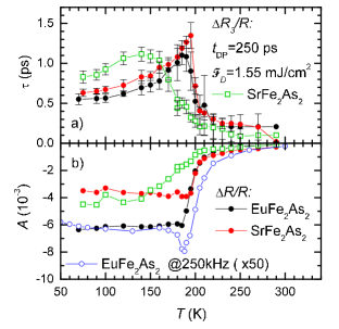
?figurename? 3: (Color online) Temperature dependence of the relaxation time and amplitude for the $\mathcal{P}^{-}$ polarization measured at 1-kHz pulse repetition rate in absence (red and black full circles) and presence of the D-pulse heating (green open squares). For comparison we plot also the amplitude $T$-dependence measured at 250-kHz repetition rate (blue open circles) at $\sim 50$ times lower pump fluence.

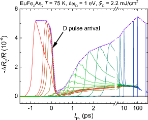
?figurename? 4: (Color online) The $\mathcal{P}^{-}$ multi-pulse transient reflectivity in Eu-122 in the presence of the destruction pulse arriving at $t_{\mathrm{D}}=0$ ps for different pump pulse arrival times measured with the 250-kHz repetition rate laser system. The dashed line represents the trajectory defined in text.

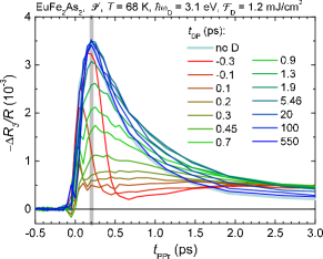
?figurename? 5: (Color online) Example of the multi-pulse transient reflectivity in Eu-122 at different $t_{\mathrm{DP}}$ plot relative to the pump arrival time, $t_{\mathrm{P}}$, measured with the 1-kHz repetition rate laser system. The vertical gray line indicates the trajectory readout pump-probe delay.

IV Multi pulse results

IV.1 Multi-pulse trajectories

In Fig. 4 we plot results of a typical multi-pulse experiment where the destruction pulse arrives at $t_{\mathrm{D}}=0$ ps, while the pump-pulse and probe-pulse arrival times are varied. By tracking the value of $\Delta R_{3}(t_{\mathrm{Pr}},t_{\mathrm{P}},t_{\mathrm{D}})$ at a constant $t_{\mathrm{PPr}}=t_{\mathrm{Pr}}-t_{\mathrm{P}}$ at the extremum ($t_{\mathrm{PPr}}\sim 200$ fs) of the unperturbed $\Delta R/R$ (Fig. 5), we define the trajectory, $A_{3}(t_{\mathrm{DP}})$, where $t_{\mathrm{DP}}=t_{\mathrm{P}}-t_{\mathrm{D}}$ is the delay between the D and P pulse. Due to the finite $t_{\mathrm{PPr}}$ at the readout of $A_{3}(t_{\mathrm{DP}})$ the temporal resolution of the trajectory is limited to $\sim t_{\mathrm{PPr}}\approx 200$ fs.

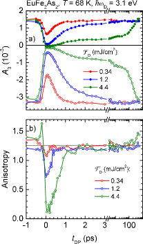
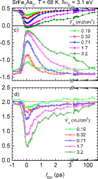
?figurename? 6: (Color online) The trajectories for the $\mathcal{P}^{+}$ (full symbols) and $\mathcal{P}^{-}$ (open symbols) polarizations at a few characteristic destruction-pulse fluences in Eu-122 (a) and Sr-122 (c). Anisotropy (see text for definition) of the trajectories at different destruction fluences in Eu-122 (b) and Sr-122 (d).

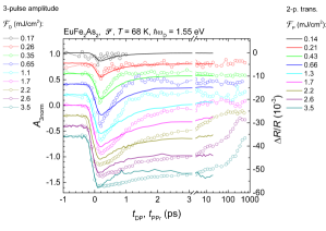
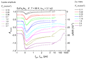
?figurename? 7: (Color online) Comparison of the normalized $\mathcal{P}^{-}$ trajectories (open symbols) to the $\mathcal{P}^{-}$ transient reflectivity (full lines) at different destruction/pump fluences in Eu-122 for two different pump/destruction photon energies.

In Fig. 6 (a) and (c) we plot typical trajectories for both probe polarizations at $T\sim 70$ K. Below $\mathcal{F}_{\mathrm{D}}\sim 1$ mJ/cm² the trajectories indicate a recovery of the ordered state on the sub-ps timescale. Above $\mathcal{F}_{\mathrm{D}}\sim 2$ mJ/cm² the recovery timescale slows down beyond hundreds of picoseconds. In the intermediate region 1 mJ/cm² $\lesssim\mathcal{F}_{\mathrm{D}}\lesssim 2$ mJ/cm² the recovery is still observed on a few ps timescale. Since the heat can not diffuse out of the excited sample volume on this timescale this indicates that the transient lattice temperature does not exceed $T_{\mathrm{N}}$ below $\mathcal{F}_{\mathrm{D}}\sim 2$ mJ/cm². This fluence therefore represents the boundary between the fast-quench and the slow-quench conditions.

In Fig. 6 (b) and (d) we plot also the anisotropy defined as ($A_{3\mathcal{P}+}-A_{3\mathcal{P}-})/(A_{3\mathcal{P}+}-A_{3\mathcal{P}-})$. In Eu-122 the anisotropy recovers on the sub-ps timescale even at the slow quench conditions while in Sr-122 the initial sub-ps recovery is followed by a slower tail lasting more than $\sim 10$ ps.

In Fig. 7 we also compare the trajectories to the standard transient reflectivity measured at similar excitation fluences. In the case of fast quench, $\mathcal{F}_{\mathrm{D}}\lesssim 2$ mJ/cm², the trajectories recover faster than the corresponding transient reflectivity for both D-photon energies. In the case of extremely slow quench, $\mathcal{F}_{\mathrm{D}}\gtrsim 2$ mJ/cm², the trajectory dynamics shows only the slow recovery while the transient reflectivity still displays a partial initial sub-picosecond relaxation.

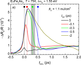
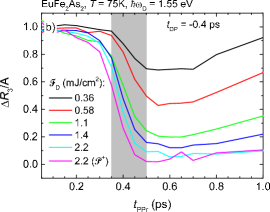
?figurename? 8: (Color online) (a) The $\mathcal{P}^{-}$ multi-pulse transient reflectivity in Eu-122 at different destruction pulse arrival times $t_{\mathrm{DP}}$. The timescale of the transient reflectivity suppression region of 150 fs for $t_{\mathrm{DP}}=0.3$ ps is indicated by the shaded region. (b) The relative suppression of the $\mathcal{P}^{-}$ $\Delta R_{3}$ as a function of $\mathcal{F}_{\mathrm{D}}$ for the destruction pulse arriving at $t_{\mathrm{DP}}=-0.4$ ps.

IV.2 Destruction timescale

To determine the destruction timescale of the ordered state we chose a negative $t_{\mathrm{DP}}$ and analyze the suppression of $\Delta R_{3}/R$ after the D pulse arrival. As shown in Fig. 8 $\Delta R_{3}/R$ is suppressed within $\sim 150$ fs at $1.55$-eV D-photon energy. The suppression timescale does not depend on $\mathcal{F}_{\mathrm{D}}$ although we observe an earlier onset of the suppression at higher $\mathcal{F}_{\mathrm{D}}$. The effect can be attributed to the wing of the D pulse extending beyond $\sim 50$ fs that at higher $\mathcal{F}_{\mathrm{D}}$ contains enough energy to start the ordered-state suppression prior to the arrival of the central part of the D pulse.

Comparing the trajectories measured at different destruction-photon energies in Fig. 7 we observe a sharper feature around the maximal-suppression $t_{\mathrm{DP}}$ in the case of the degenerate, $\hbar\omega_{\mathrm{D}}=1.55$ eV, D-photon energy. While the suppression timescale appears identical for both D-photon energies in Eu-122 the suppression at 3.1-eV D-photon energy in Sr-122 appears slower [Fig. 9 (b)] consistent with the slower risetime in the standard pump-probe experiment [Fig. 2 (h)].

V Analysis and Discussion

V.1 Destruction-pulse absorption saturation

The large difference between experimentally determined transient lattice heating and the estimate based on the equilibrium optical and thermodynamic properties indicates that the D-pulse energy $\sim 250$ ps after the pulse arrival is deposited in a layer that is about $\sim 3$ times thicker than the optical penetration depth ($\sim 20-30$ nm) at the highest fluences used. This large energy deposition depth can neither be accounted for by the thermal diffusion on the $\sim 250$ ps timescale nor the initial ballistic photoexcited carrier transport. The most plausible explanation that remains is therefore saturation of absorption. This is supported also by the fact that the multipulse trajectories (see Fig. 7) show a sharp feature near $t_{\mathrm{DP}}=0$ when the pump and destruction photon energies are degenerate.

V.2 Three temperature model simulations of recovery

In all-optical experiments it is generally not possible to directly disentangle dynamics of different degrees of freedom due to unknown response functions. In general, both $\Delta R$ and $A_{3}$ can couple to single particle and order parameter excitations. We therefore seek better insight into the recovery by means of semi-empirical simulations similar as previously in the cuprate superconductors.Madan et al. (2016, 2017)

At low excitation densities the order parameter as well $\Delta R$ can usually be linearly expanded in terms of a single parameter that is used to describe the nonequilibrium electronic distribution function (NEDF) dynamics. In the present compounds we have conjectured that the low-excitation transient reflectivity couples to the collective SDW order parameter that has fast femtoseconds-timescale dynamics. In such case the order parameter and transient reflectivity directly follow the magnon-bottleneck governed NEDF dynamics.Pogrebna et al. (2014)

At high excitation densities the relation between the NEDF and order parameter becomes nonlinear and the simple low-excitation description of $\Delta R$ is expected to break down. This is indicated by the difference between the relaxation dynamics (Fig. 7) observed in the standard pump-probe and multi-pulse experiments that suggests that NEDF and the order parameter have different delay dependence.

	$\eta$	$\gamma_{\mathrm{e}}$	$G_{\mathrm{eo}}$	$\lambda\left\langle\omega^{2}\right\rangle$	$c_{\mathrm{E}0}$	$G_{\mathrm{ol}}$	$k=\kappa/V_{\mathrm{mol}}$	$L_{\mathrm{D}}/\mathcal{F}_{\mathrm{D}}$
	-	mJ/mol K2	TW/mol K	(meV)2	J/mol K	TW/mol K	W/m K	nm cm2/mJ
Eu-122 (TR-ARPES)Rettig et al. (2013) ($T\sim 100$ K)	$0.01$	$52\pm 3$	$34\pm 3$	$39\pm 3$	$67\pm 14$	$7\pm 5$	-	17
	0.5	$30\pm 2$	$23\pm 3$	$45\pm 3$	$76\pm 20$	$11\pm 9$	-	17
Eu-122 (present work)
($T\sim 70$ K)	Fig. 10	$49\pm 1$	$13\pm 1$	$16\pm 2$	$10\pm 1$	Fig. 10	$14\pm 1$	$17\pm 5$
Sr-122 (present work)
($T\sim 70$ K)	Fig. 10	$57\pm 2$	$16\pm 1$	$17\pm 2$	$24\pm 1$	Fig. 10	$10\pm 1$	$23\pm 5$

?tablename? 1: Comparison of the three temperature model parameters obtained from fits. The detailed definition of the parameters is given in Section VII.2.

In the cuprate superconductors the characteristic timescale of the order parameter relaxation appears to beMadan et al. (2016, 2017) on a picosecond timescale and the intrinsic order parameter dynamics plays an important role on the experimental-observation timescale. In the present case the SDW order parameter is expected to relax much faster due to a larger gap ($2\Delta_{\mathrm{SDW}}\sim 200$ meVPogrebna et al. (2014)). An estimate of the SDW amplitude mode frequency,Psaltakis (1984) $\omega_{\mathrm{AM}}=2\Delta_{\mathrm{SDW}}/\hbar$, would lead to the relaxation timescale bottom limit of $\sim 3$ fs. On the other hand, the SDW transition is coupled to the structural transition that could lead to renormalization and slowdown of the order parameter relaxation timescale. Recent time resolved X-ray diffraction experimentsGerber et al. (2015); Rettig et al. (2016) showed, however, that on the tens of picoseconds timescale the orthorhombic lattice splitting is decoupled from the electronic order parameter.

In the present multi-pulse experiments the time resolution of the trajectories is not better than the risetime of the standard pump-probe response ($\sim 200$ fs). Any intrinsic order parameter dynamics faster than $\sim 200$ fs would therefore not be revealed in the experiment. Since it is very likely that the intrinsic order parameter relaxation timescale is faster than the resolution we check this hypothesis by simulating the trajectories assuming that the order parameter and the optical response directly follow the NEDF on the experimentally accessible timescales.

Since modeling of the NEDF dynamics in strongly excited collectively ordered systems such are SDWs is prohibitively difficult we further assumeRettig et al. (2013) that NEDF can be approximately described by an electronic temperature. To calculate the optical response we use an empirical response function assuming and that the amplitude of the pump-pulse induced transient dielectric constant, $\Delta\epsilon_{3}^{\mathrm{A}}(z,t_{\mathrm{DP}})$, depends on the local electronic temperature, $T_{\mathrm{e}}(z,t_{\mathrm{DP}})$, only,

$$\Delta\epsilon_{3}^{\mathrm{A}}(z,t_{\mathrm{DP}})\propto A(T_{\mathrm{e}}[z,t_{\mathrm{DP}}]).$$ (2)

Here $A(T)$ is the experimental $T$-dependent amplitude measured in the absence of the D pulse shown in Fig. 3 (b) and $z$ corresponds to the normal distance from the sample surface. For the sake of simplification any radial dependence is neglected. The multipulse transient reflectivity amplitude is given by (see Appendix VII.1):

$$A_{3}(t_{\mathrm{DP}}) \propto\int_{0}^{\infty}dz e^{-\alpha_{\mathrm{Pr}}z}\cos\left(2n_{\mathrm{Pr}}\frac{\omega_{0}}{c_{0}}z-\phi\right)\Delta\epsilon_{3}^{\mathrm{A}}(z,t_{\mathrm{DP}}),$$ (3)

where $\alpha_{\mathrm{Pr}}$ and $n_{\mathrm{Pr}}$ are the probe absorption coefficient and the real part of the refraction index, respectively. The phase $\phi$ depends (see Appendix, Eq. (18)) on the static complex refraction index and the ratio between the real and imaginary part of $\Delta\epsilon_{3}^{\mathrm{A}}$.

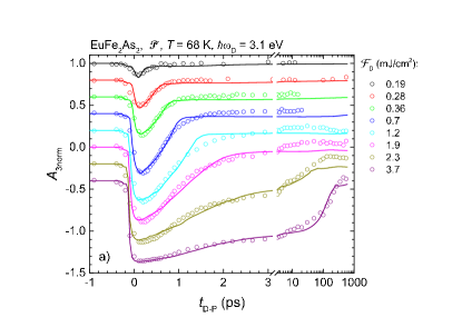
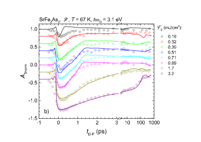
?figurename? 9: (Color online) Comparison of the experimental (open circles) and simulated (lines) trajectories for the case of $\phi=\pi/2$. The trajectories at different $\mathcal{F}_{\mathrm{D}}$ are vertically shifted for clarity.

Since $A(T)$ is virtually temperature independent in the SDW state dropping abruptly above $T_{\mathrm{SDW}}$ the trajectories, $A_{3}(t_{\mathrm{DP}}),$ are expected to reflect mainly the SDW volume-fraction dynamics in the probed volume and/or the normal/nematic-state dynamics when the SDW state is completely suppressed. Since $A(T)\rightarrow 0$ above $\sim 300$ K the sensitivity in the later case is limited to the temperature window between $\sim 200-\sim 300$ K.

The evolution of $T_{\mathrm{e}}(z,t_{\mathrm{DP}})$ after the D pulse is calculated solving a three temperature modelPerfetti et al. (2007); Rettig et al. (2013), where a subset of optical phonons with temperature, $T_{\mathrm{o}}$, different from the lattice temperature, $T_{\mathrm{L}}$, is assumed to be strongly coupled to the electronic subsystem. In the simplest 3TM it is also assumed that all the absorbed energy remains in the electronic subsystem until it completely thermalizes. Here the model is extended assuming that a part, $\eta$, of the absorbed energy is transferred directly to a few strongly coupled optical phonons during thermalization of the NEDF on a few-$100$-fs timescale.Demsar et al. (2003)

To fit the simulated trajectories to the experimental data we take the experimental specific heat capacity, $c_{\mathrm{p}}(T)$,Herrero-Martín et al. (2009); Chen et al. (2008), and set $\phi$ in Eq. (3) to the either 0 or $\pi/2$. We also fix the heating pulse length to 200 fs corresponding to the trajectory temporal resolution. The rest of the 3TM parameters are determined from the nonlinear least squares fit. In the first step only the trajectories for the highest $\mathcal{F}_{\mathrm{D}}$ are fit. Due to rather accurate total specific-heat-capacityHerrero-Martín et al. (2009); Chen et al. (2008) and static optical-reflectivity dataCharnukha et al. (2013); Wu et al. (2009) the thermal conductivity, $k,$ and the phenomenological D-pulse saturated-absorption length, $L_{\mathrm{D}}\sim 80$ nm, at the highest $\mathcal{F}_{\mathrm{D}}$ are obtained from the long DP-delay behavior in both samples.

To fit the lower-$\mathcal{F}_{\mathrm{D}}$ trajectories it is assumed that $L_{\mathrm{D}}\propto\mathcal{F}_{\mathrm{D}}$ while a global fit over all trajectories at different $\mathcal{F}_{\mathrm{D}}$ is used to determine the remaining parameters. With all the fit parameters taken to be independent of $\mathcal{F}_{\mathrm{D}}$ it is not possible to obtain reasonable fits at all experimental $\mathcal{F}_{\mathrm{D}}$s simultaneously since the 3TM model results in too strong slowdown of the relaxation with increasing $\mathcal{F}_{\mathrm{D}}$. On the other hand, assuming that $G_{\mathrm{ol}}$ and $\eta$ depend on $\mathcal{F}_{\mathrm{D}}$ and setting $\phi=\pi/2$ results in excellent fits (shown in Fig. 9) in the complete experimental $\mathcal{F}_{\mathrm{D}}$ range. The quality of the fits supports the initial hypothesis of the fast sub 200-fs order parameter dynamics.

The obtained 3TM fit parameters are shown in Table V.2 and Fig. 10. For comparison the fit parameters from fits to the published time resolved -ARPESRettig et al. (2013) (TR-ARPES) surface-$T_{\mathrm{e}}$ dynamics in Eu-122 are also shown.

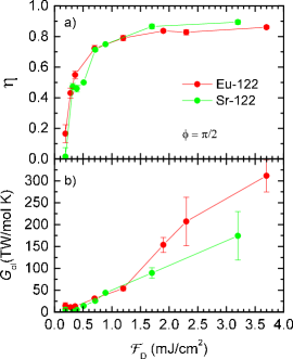
?figurename? 10: (Color online) The destruction-pulse fluence dependence of the branching factor (a) and the electron - optical-phonons coupling (b) from the 3TM fit.

The obtained normal-state values of the electronic specific heat constant, $\gamma_{\mathrm{e}}$, in the 50-60 mJ/mol K² range (Table V.2) are significantly larger than the low-temperature (SDW-state) thermodynamic value of $\gamma_{\mathrm{e}}\sim 8$ mJ/mol K² Chen et al. (2008). The increase of $\gamma_{\mathrm{e}}$ in the normal state is consistent with the suppression of the SDW gap, but appears somewhat larger than upon suppression of the SDW state by Co dopingHardy et al. (2010) in Ba-122, where $\gamma_{\mathrm{e}}$ increases from $\sim 5$ mJ/mol K² in the SDW state to $\sim 25$ mJ/mol K² in the superconducting samples. On the other hand, assuming that the high normal state magnetic susceptibilityJohnston (2010) is dominated by the Pauli contribution and the electron-phonon coupling constant is smallStojchevska et al. (2010, 2012) results in comparable $\gamma_{\mathrm{e}}\sim 60$ mJ/mol K².

While the values of $\gamma_{\mathrm{e}}$ for Eu-122 obtained from our data and TR-ARPES are consistent there is much larger discrepancy of the other parameters. Fits to the multipulse trajectories result in a smaller electron phonon relaxation rate, $G_{\mathrm{eo}}$, larger optical-phonon - lattice relaxation rate, $G_{\mathrm{ol}}$, and significantly smaller strongly-coupled optical-phonon heat capacity. Partially this can be attributed to the systematic errors of the 3TM and the response function. Setting $\eta$ to a fixed $\mathcal{F}_{\mathrm{D}}$-independent value results in qualitatively similar trajectories (see Appendix VII.3, Fig. 13 and Table. VII.3) with similar $\gamma_{\mathrm{e}}$ and $c_{\mathrm{E0}}$, but significantly different relaxation rate parameters. Another obvious contribution to the difference are also differences between the surface and bulk since the present technique is more bulk sensitive than TR-ARPES.

By using a simpler two temperature model with $\mathcal{F}_{\mathrm{D}}$-dependent $\gamma_{\mathrm{e}}$ and the electron phonon coupling it is also possible to obtain fair fits to the trajectories (not shown). However, from such fits an nonphysically large $\gamma_{\mathrm{e}}$ of $\sim 200$  mJ/mol K² is obtained indicating that some strongly coupled optical phonons must play a role in the energy relaxation. It therefore appears that the dominant relaxation bottleneck is cooling of the strongly-coupled optical phonons to the lattice bath.

$\mathcal{F}_{\mathrm{D}}$-dependence of the optical-phonons - lattice relaxation rate, $G_{\mathrm{ol}}$, shows a strong increase with increasing $\mathcal{F}_{\mathrm{D}}$ (see Fig. 10). The increase is robust to the variations of the branching-factor fitting approach (see Appendix VII.3, Fig. 14) and can be attributed to opening of additional electronic relaxation channels upon suppression of the nematic-fluctuations related pseudogapStojchevska et al. (2012) in addition to the anharmonic-decay channels.

A less robust result of our analysis is the increase of the branching factor, $\eta$, with increasing $\mathcal{F}_{\mathrm{D}}$ suggesting that above $\mathcal{F}_{\mathrm{D}}\sim 1$ mJ/cm² the majority of the absorbed optical energy is on $\sim 100$-fs timescale transferred to the strongly coupled optical phonons. This is corroborated with a quick initial recovery of the anisotropy (Fig. 6) that indicates that $T_{\mathrm{e}}$ drops below $\sim 300$ K into the region of strong nematic fluctuations already a few hundred fs after the arrival of the D-pulse. While the increase of $\eta$ appears correlated with the observed optical nonlinearity we could not come up with any persuasive physical picture to explain the effect so we leave it open for further experimental confirmation and discussion.

V.3 Destruction timescale

The experimental destruction timescale of $\sim 150$ fs could be set either by the intrinsic low-energy SDW order parameter dynamics or the finite initial NEDF thermalization timescale. While the intrinsic SDW order dynamics on the $\sim 150$-fs timescale would not contradict the 3TM simulation results, the dependence of the destruction timescale on the D-photon energy in Sr-122 suggests that the destruction timescale is set by the initial NEDF thermalization.

V.4 Determination of the SDW destruction threshold

As in superconductors and charge density wavesStojchevska et al. (2011) we associate the saturation of the transient reflectivity amplitude in the standard pump-probe experiments with destruction of the ordered state. In the present case the saturation is incomplete where the finite slope at high excitation density presumably corresponds to the transient response of the normal, unordered state.

The shape of the saturation curve [see Fig. 2 (c) and (g)] depends on the SDW destruction threshold excitation energy density, $U{}_{\mathrm{th}}$, the geometrical parameters of the pump and probe beams and their penetration depths. In addition, the contribution of the pump-absorption saturation has to be taken into account in the present case.

To take into account the above effects we formulate a simple phenomenological saturation model where we approximate the local amplitude of the transient change of the dielectric constant, $\Delta\epsilon(r,z)$, by a piece-wise linear function of the locally absorbed energy density, $U(r,z)$, that has different slopes below and above $U{}_{\mathrm{th}}$:

$$\Delta\epsilon(r,z) = \Delta\epsilon_{0}g(r,z),$$

$$g(r,z) = \begin{cases}\frac{U(r,z)}{U_{\mathrm{th}}};&U(r,z)<U_{\mathrm{th}}\\ 1+a(\frac{U(r,z)}{U_{\mathrm{th}}}-1);&U(r,z)\geq U_{\mathrm{th}}\end{cases},$$ (4)

where $r$ corresponds to the radial distance from the beam center, $z$ the normal distance from the sample surface and $a$ to the relative slope in the normal state. The spatial dependence of $U(r,z)$ is given by:

$$\frac{U(r,z)}{U_{\mathrm{th}}} = \frac{\mathcal{F}_{0}}{\mathcal{F}_{\mathrm{th}}}\frac{\left(1+e^{-\alpha_{\mathrm{P}}L_{\mathrm{P}}(\mathcal{F}_{\mathrm{th}},0)}\right)e^{-2r^{2}/\rho_{\mathrm{P}}^{2}}}{\left(1+e^{\alpha_{\mathrm{P}}[z-L_{\mathrm{P}}(\mathcal{F}_{0},r)]}\right)},$$ (5)

$$L_{\mathrm{P}}(\mathcal{F},r) = c_{\alpha}\mathcal{F}e^{-2r^{2}/\rho_{\mathrm{P}}^{2}},$$ (6)

where $\alpha_{\mathrm{P}}$ is the linear pump absorption coefficient. We phenomenologically take into account the pump-absorption saturation by using the Fermi function to model the $U(r,z)$ depth dependence introducing the local fluence dependent pump-penetration depth (6). The coefficient, $c_{\alpha}$, is determined from the multi-pulse experiment fits discussed above, while the pump beam is characterized by the pump beam diameter, $\rho_{\mathrm{P}}$, and the external fluence in the center of the beam, $\mathcal{F}_{0}$. $\mathcal{F}_{\mathrm{th}}$ corresponds to the external threshold fluence at which $U{}_{\mathrm{th}}$ is reached at the surface ($z=0$) in the center of the beam ($r=0$).

$\hbar\omega_{\mathrm{P}}$	1.55 eV		3.1eV
$\phi$	0	$\pi/2$	0	$\pi/2$
	$\mathcal{F}_{\mathrm{th}}$ (mJ/cm2)
EuFe2As2	0.21	0.15	0.18	0.12
SrFe2As2	0.21	0.16	0.20	0.16

?tablename? 2: The external destruction threshold fluence, $\mathcal{F}_{\mathrm{th}}$ at different pump photon energies, $\hbar\omega_{\mathrm{P}}$ for two extreme phase shifts $\phi$. The static optical constants used in fits were taken from Refs. [Wu et al., 2009] and [Charnukha et al., 2013].

In the case of a relatively wide Gaussian probe beam with diameter $\rho_{\mathrm{Pr}}$ Eq. (3) describing the transient-reflectivity amplitude can be simply upgraded to take into account the radial variation of the response (see also Appendix VII.1):

$$A \propto\int_{0}^{\infty}rdr\int_{0}^{\infty}dz e^{-2r^{2}/\rho_{\mathrm{Pr}}^{2}}e^{-\alpha_{\mathrm{Pr}}z}\cos\left(2n\frac{\omega_{0}}{c_{0}}z-\phi\right)g(r,z).$$ (7)

When fitting Eq. (7) to the experimental data it turns out that $\mathcal{F}_{\mathrm{th}}$, $\phi$ and $a$ are strongly correlated. Since $\phi$ is usually not known a priori we fix $\phi$ to either 0 or $\pi/2$ to obtain a range of values for $\mathcal{F}_{\mathrm{th}}$. Example fits with $\phi=\pi/2$, are shown in Fig. 2 (c) and (g) with the resulting $\mathcal{F}_{\mathrm{th}}$ shown in Table 2. While the variation of $\phi$ can strongly influence the extracted $\mathcal{F}_{\mathrm{th}}$ the determined ranges of $\mathcal{F}_{\mathrm{th}}$ are very similar in both samples at both pump-photon energies.

Taking $\phi=\pi/2$ indicated by the 3TM simulations (Table 2) we calculate the destruction treshold energy density, $U_{\mathrm{th}}\sim 1.6$ kJ/mol for Eu-122 and $U_{\mathrm{th}}\sim 2.5$ kJ/mol for Sr-122. Assuming that $U_{\mathrm{th}}$ corresponds to the condensation energy and taking $\gamma_{\mathrm{e}}$ from the 3TM fits we can estimate the SDW gap using the standard BCS formula and obtain $\nicefrac{{2\Delta_{\mathrm{SDW}}}}{{k_{\mathrm{B}}T_{\mathrm{SDW}}}}=5$ and 6 for Eu-122 and Sr-122, respectively. This is somewhat lower than the earlier weak-excitation pump-probe estimatePogrebna et al. (2014) of 13 and 8 for Eu-122 and Sr-122, respectively, but closer to the optical conductivity result of 5.6 in Eu-122 Wu et al. (2009).

Contrary to the superconductorsStojchevska et al. (2011); Beyer et al. (2011) there is no indication that the optical destruction energy would significantly exceed the estimated SDW condensation energy. This is consistent with the 3TM trajectories fit results where at small $\mathcal{F}_{D}$ that is comparable to $\mathcal{F}_{\mathrm{th}}$ the fast optical energy transfer to the phonons is rather small (Fig. 10).

VI Summary and conclusions

We presented an extensive all-optical study of the transient SDW state suppression and recovery in EuFe₂As₂ and SrFe₂As₂ under strong ultrafast optical excitation by means of the standard time resolved pump-probe as well as the multi-pulse transient optical spectroscopy.

The SDW order is suppressed on a $\sim 150$ - $\sim 250$-fs timescale after a $50$-fs destruction optical pulse absorption, depending on the optical-photon energy. The suppression time scale is fluence independent and set by the initial electronic thermalization timescale.

The SDW recovery timescale increases with the destruction optical-pulse fluence, but remains below $\sim 1$ ps up to the fluence at which the transient lattice temperature exceeds the SDW transition temperature.

The optical SDW destruction threshold energy densities of $\sim 1.6$ kJ/mol and $\sim 2.5$ kJ/mol in EuFe₂As₂ and SrFe₂As₂, respectively, are consistent with the BCS condensation energy estimates.

The time evolution of the multi-pulse system trajectories in a broad destruction-pulse fluence range can be well described within the framework of an extended three temperature model assuming a fast sub 200-fs intrinsic order parameter timescale. The model fits indicate the normal state specific heat constant, $\gamma_{\mathrm{e}}$, in the 50-60 mJ/mol K² range. The fluence-dependent recovery timescale is found to be governed by the optical-phonons - lattice relaxation bottleneck that is strongly suppressed at high excitation densities. The suppression of the bottleneck is attributed to a suppression of the the nematic-fluctuations induced pseudogap at high temperatures.

The observed resilience of the SDW state at high fluences exceeding the SDW-destruction threshold fluence of $\sim 0.15$ mJ/cm² up to $\sim 10$ times is attributed to saturation of the optical absorption. The model fits also suggest that at these fluences the majority of the absorbed optical energy is transferred to the optical phonons during the initial electronic thermalization on a few hundred femtosecond time scale.

VII Appendix

VII.1 Transient reflectivity

Assuming that the beam diameters are large in comparison to the optical penetration depth and the transient dielectric constant varies slowly on the optical pulse timescale, $\Delta\epsilon(z,t)\sim\Delta\epsilon(z)$, we can write the wave equation for the perturbed probe field in one dimension:

$$\frac{\mathcal{N}^{2}}{c_{0}^{2}}\frac{\partial^{2}\Delta E}{\partial t^{2}}-\frac{\partial^{2}\Delta E}{\partial z^{2}}=-\frac{1}{\epsilon_{0}c_{0}^{2}}\frac{\partial^{2}\Delta P}{\partial t^{2}},$$ (8)

where $t$ is time, $z$ the distance from the sample surface, $\mathcal{N}=n+i\kappa$ the complex refraction index, $\Delta P$ the pump-probe induced transient polarization with $c_{0}^{2}$ and $\epsilon_{0}$ the speed of light and the vacuum permittivity, respectively. In the presence of a monochromatic probe field, $E_{\mathrm{Pr}}(z,t)=t_{12}E_{\mathrm{0Pr}}e^{-i(\omega t-\mathcal{N}kz)}+\mathrm{c.c.}$, propagating into the sample the transient polarization is given by:

$$\Delta P(z) = \epsilon_{0}\Delta\epsilon(z)E_{\mathrm{Pr}}(z,t)=,$$ (9)

$$= t_{12}E_{\mathrm{0Pr}}\epsilon_{0}\Delta\epsilon(z)e^{-i(\omega t-\mathcal{N}\frac{\omega}{c_{0}}z)}+\mathrm{c.c.}$$

where $E_{\mathrm{0Pr}}$ is the complex amplitude of the incident probe field at the sample surface (at $z=0$) and $t_{12}=2/(1+\mathcal{N})$ is the Fresnel transmission coefficient. Solving (8) assuming (9) we obtain to the linear order in $\Delta\epsilon(z)$ the transient reflected field outside of the sample (at $z=0$):

$$\Delta E_{\mathrm{r}}=\frac{i}{2}\frac{t_{12}t_{21}\omega}{c_{0}\mathcal{N}}E_{\mathrm{Pr0}}e^{-i\omega t}\int_{0}^{\infty}\Delta\epsilon(z)e^{2i\mathcal{N}\frac{\omega}{c_{0}}u}dz+\mathrm{c.c.},$$ (10)

where the Fresnel coefficient $t_{21}=2\mathcal{N}/(1+\mathcal{N})$ takes into account the transmission from the sample to vacuum.

In the case of an incident Gaussian probe pulse:

$$E_{\mathrm{Pr}}^{\mathrm{pulse}}(t) =A_{0} \sqrt{\frac{2}{\tau\sqrt{\pi}}}e^{-2t^{2}/\tau^{2}}e^{-i\omega_{0}t}+\mathrm{c.c.}=$$ (11)

$$= \int_{0}^{\infty}A(\omega-\omega_{0})e^{-i\omega t}d\omega+\mathrm{c.c.},$$

the total transient reflected electric field, neglecting the dispersion, is the integral:

$$\Delta E_{\mathrm{r}}^{\mathrm{pulse}}(t) = \frac{i}{2}\frac{t_{12}t_{21}}{c_{0}\mathcal{N}}\int_{0}^{\infty}dz\Delta\epsilon(z)\int_{0}^{\infty}d\omega\omega A(\omega-\omega_{0})e^{-i\omega t}e^{2i\mathcal{N}\frac{\omega}{c_{0}}z}+\mathrm{c.c.}=$$ (12)

$$= -\frac{t_{12}t_{21}A_{0}}{2\sqrt{2}\sqrt[4]{\pi}c_{0}\mathcal{N}\sqrt{\tau}}\frac{\partial}{\partial t^{\prime}}\left[\int_{0}^{\infty}\Delta\epsilon(z)e^{-2t^{\prime 2}/\tau^{2}}\times\right.$$

$$\left.\times\left[e^{-i\omega_{0}t^{\prime}}\left(1+\mathrm{erf}\left[\frac{\omega_{0}\tau}{2\sqrt{2}}+i\sqrt{2}\frac{t^{\prime}}{\tau}\right]\right)+e^{i\omega_{0}t^{\prime}}\left(1-\mathrm{erf}\left[\frac{\omega_{0}\tau}{2\sqrt{2}}-i\sqrt{2}\frac{t^{\prime}}{\tau}\right]\right)\right]dz\right]+\mathrm{c.c.}\approx$$

$$\approx -\frac{t_{12}t_{21}A_{0}}{2\sqrt[4]{\pi}c_{0}\mathcal{N}\sqrt{\tau}}\frac{\partial}{\partial t}\left[\int_{0}^{\infty}\Delta\epsilon(z)e^{-2(t-2\mathcal{N}z/c_{0})^{2}/\tau^{2}}e^{-i\omega_{0}(t-2\mathcal{N}z/c_{0})}du\right]+\mathrm{c.c.},$$

where $t^{\prime}=t-2\mathcal{N}z/c_{0}$. In the last line we assumed that the pulse is narrowband, $\omega_{0}\tau\gg$1, so,

$$\left|t^{\prime}\right|/\tau\ll\omega_{0}\tau.$$ (13)

The transient reflectivity is then given by:

$$\frac{\Delta R}{R} = \frac{\Delta I_{\mathrm{r}}}{I_{\mathrm{r}}}\simeq\frac{2\int\Re(\Delta E_{\mathrm{r}}^{\mathrm{pulse}}E_{\mathrm{r}}^{*})dt}{\int E_{\mathrm{r}}E_{\mathrm{r}}^{*}dt}=$$ (14)

$$= \Re\left[-\frac{t_{12}t_{21}}{\sqrt{\pi}c_{0}r_{12}\mathcal{N}\tau}\int dte^{-2t^{2}/\tau^{2}}e^{i\omega_{0}t}\times\right.$$

$$\left.\times\frac{\partial}{\partial t}\int_{0}^{\infty}dz\Delta\epsilon(z)e^{i\omega_{0}(2\mathcal{N}z/c_{0}-t)}e^{-2(2\mathcal{N}z/c_{0}-t)^{2}/\tau^{2}}\right]=$$

$$= \Re\left[-\frac{\omega_{0}t_{12}t_{21}}{2c_{0}r_{12}\mathcal{N}}\int_{0}^{\infty}dz\Delta\epsilon(z)e^{2i\frac{\omega_{0}}{c_{0}}\mathcal{N}z}K(z)\right],$$

$$K(z) = \left(1+i\frac{4\mathcal{N}z}{\omega_{0}c_{0}\tau^{2}}\right)e^{-4\mathcal{N}^{2}z^{2}/c_{0}^{2}\tau^{2}},$$ (15)

where $E_{\mathrm{r}}=r_{12}E_{\mathrm{Pr}}^{\mathrm{pulse}}(t)$ and $r_{12}=(1-\mathcal{N})/(1+\mathcal{N})$ is the reflection coefficient. In comparison to the CW case (10) an additional term $K(z)$ appears in the kernel of the integral (14). Due to the exponent the kernel in (14) decays on the length scale $z\sim c_{0}/\omega_{0}\mathcal{\kappa}$ satisfying the condition (13) when $\omega_{0}\tau\gg\sqrt{n^{2}/\kappa^{2}+1}$. On this length scale the argument of the exponent in (15) is of the order $4\left|\mathcal{N}\right|^{2}/\kappa^{2}\omega_{0}^{2}\tau^{2}\ll 1$ for the narrowband pulses satisfying $\omega_{0}\tau\gg\sqrt{n^{2}/\kappa^{2}+1}$ so $K(z)\sim 1$ can be dropped from (14).

Due to the phase factor in (14) the real and imaginary parts of $\Delta\epsilon(z)=\Delta\epsilon_{\mathrm{r}}(z)+i\Delta\epsilon_{\mathrm{i}}(z)$ show different depth sensitivity that depends on the static complex refraction index:

$$\frac{\Delta R}{R} = \frac{4\omega_{0}}{c_{0}\left|\mathcal{N}^{2}-1\right|}\int_{0}^{\infty}dze^{-\alpha_{\mathrm{Pr}}z}\left[\Delta\epsilon_{\mathrm{r}}(z)\sin\left(2n\frac{\omega_{0}}{c_{0}}z-\beta\right)+\Delta\epsilon_{\mathrm{i}}(z)\cos\left(2n\frac{\omega_{0}}{c_{0}}z-\beta\right)\right],$$ (16)

$$\tan(\beta) = \frac{\Im(\mathcal{N}^{2}-1)}{\Re(\mathcal{N}^{2}-1)}=\frac{2n\kappa}{n^{2}-\kappa^{2}-1},$$

where, $\alpha_{\mathrm{Pr}}=2\kappa\frac{\omega_{0}}{c_{0}}$, is the probe absorption coefficient.

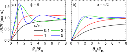
?figurename? 11: (Color online) Simulated fluence dependence for the case of Gaussian beams from Eq. (7) for different ratios $n/\kappa$ for two orthogonal phase shifts, $\phi$, taking $\rho_{\mathrm{P}}/\rho_{\mathrm{P}r}=2$, $\alpha_{\mathrm{Pr}}/\alpha_{\mathrm{P}}=1$, $c_{\alpha}=0$ and $a=0$. The curves are normalized to the saturated value at $\mathcal{F}_{0}\gg\mathcal{F}_{\mathrm{th}}$.

Since in the simple saturation model (4) the real and imaginary parts of $\Delta\epsilon(z)$ are assumed to have the same $z$ dependence Eq. (16) is simplified to:

$$\frac{\Delta R}{R} = \frac{4\omega_{0}\left|\Delta\epsilon_{0}\right|}{c_{0}\left|\mathcal{N}^{2}-1\right|}\int_{0}^{\infty}dze^{-\alpha_{\mathrm{Pr}}z}\cos\left(2n\frac{\omega_{0}}{c_{0}}z-\phi\right)g(z),$$ (17)

$$\tan(\phi) = \frac{2n\kappa\Delta\epsilon_{0\mathrm{r}}-(n^{2}-\kappa^{2}-1)\Delta\epsilon_{0\mathrm{i}}}{2n\kappa\Delta\epsilon_{0\mathrm{i}}+(n^{2}-\kappa^{2}-1)\Delta\epsilon_{0\mathrm{r}}}.$$ (18)

In the case of Gaussian pump and probe beams with the diameters $\rho_{\mathrm{P}}$ and $\rho_{\mathrm{Pr}}$, respectively, (17) can be easily extendedKusar et al. (2008) to (7) by an additional integration in the radial direction where $g(r,z)$ is obtained from (4) by taking into account the radial pump fluence dependence.

With increasing pump fluence the boundary between the ordered and normal state region in (4) moves along $z$, so the oscillatory factor in the integral can lead to a non-monotonous excitation-density dependence of the $\Delta R/R$ when $n/\kappa\gtrsim 1$ as shown in Fig. 11. There is unfortunately no clear singularity observed when the threshold fluence is reached at low $n/\kappa$ ratios. Moreover, the saturation is much less pronounced for $\phi=\pi/2$.

VII.2 Three temperature model

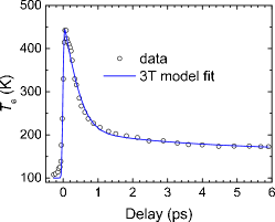
?figurename? 12: Three temperature model fit to the electronic temperature in Eu-122 from TR-ARPESRettig et al. (2013). Setting $\eta$ to different values results in virtually identical fit curves (not shown) with modified remaining 3TM parameters (see Table V.2).

The time evolution of the temperatures in the three-temperature model is governed by:

$$\gamma_{\mathrm{e}}T_{\mathrm{e}}\frac{\partial T_{\mathrm{e}}}{\partial t} = (1-\eta)s(z,t)-G_{\mathrm{eo}}(T_{\mathrm{e}}-T_{\mathrm{o}})+\kappa\frac{\partial T_{\mathrm{e}}^{2}}{\partial z^{2}},$$

$$c_{\mathrm{E}}(T_{\mathrm{o}})\frac{\partial T_{\mathrm{o}}}{\partial t} = \eta s(z,t)+G_{\mathrm{eo}}(T_{\mathrm{e}}-T_{\mathrm{o}})-G_{\mathrm{ol}}(T_{\mathrm{o}}-T_{\mathrm{l}}),$$

$$c_{\mathrm{L}}(T_{\mathrm{L}})\frac{\partial T_{\mathrm{L}}}{\partial t} = G_{\mathrm{ol}}(T_{\mathrm{o}}-T_{\mathrm{L}}),$$ (19)

where $T_{\mathrm{e}}$, $T_{\mathrm{o}}$ and $T_{\mathrm{L}}$ are the electronic, the strongly-coupled optical phonon (OP) and lattice temperatures, respectively. $\gamma_{\mathrm{e}}$ is the normal state electronic specific heat constant, $c_{\mathrm{E}}(T_{\mathrm{o}})$ the Einstein phonon specific heat and $c_{\mathrm{L}}(T_{\mathrm{L}})$ the lattice specific heat. $G_{\mathrm{eo}}$ and $G_{\mathrm{ol}}$ are the electron-OP and OP-lattice coupling constants, while $\kappa$ is the electronic heat diffusivity. $s(z,t)$ is the absorbed laser energy density rate. Using the branching factor, $\eta$, we take into account that the primary electron-hole pair can relax by exciting the optical phonons during the thermalization.

To take into account absorption saturation we approximate $s(z,t)$ by:

$$s(z,t)\propto\mathcal{F}_{\mathrm{D}}e^{-\nicefrac{{2t^{2}}}{{\tau_{\mathrm{p}}^{2}}}}\left[1+e^{\alpha_{\mathrm{D}}(z-L_{\mathrm{D}})}\right]^{-1},$$ (20)

where $\tau_{\mathrm{p}}$ is the effective heating pulse length, $\alpha_{\mathrm{D}}$ the D-pulse linear absorption coefficient and $L_{\mathrm{D}}$ the phenomenological absorption length.

$c_{\mathrm{E}}(T)$ is parametrized by the Einstein model:

$$c_{\mathrm{E}}(T)=c_{\mathrm{E}0}\left(\frac{T_{\mathrm{E}}}{T}\right)^{2}e^{\frac{T_{\mathrm{E}}}{T}}/(e^{\frac{T_{\mathrm{E}}}{T}}-1)^{2},$$ (21)

while $c_{\mathrm{L}}(T)$ is obtained from the total experimental specific heat capacityHerrero-Martín et al. (2009); Chen et al. (2008), $c_{\mathrm{p}}(T)$, by subtracting the electronic and OP parts:

$$c_{\mathrm{L}}(T)=c_{\mathrm{p}}(T)-\gamma_{\mathrm{e}}T_{\mathrm{e}}-c_{\mathrm{E}}(T).$$ (22)

According to AllenAllen (1987) the second moment of the Eliashberg function can be expressed as:

$$\lambda\left\langle\omega^{2}\right\rangle=\frac{\pi k_{\mathrm{B}}}{3\hbar}\frac{G_{\mathrm{eo}}}{\gamma_{\mathrm{e}}}.$$

VII.3 3TM fits with a single $\mathcal{F}_{\mathrm{D}}$-dependent parameter

A worse fit, particularly at low $\mathcal{F}_{\mathrm{D}}$, with fixed and $\mathcal{F}_{\mathrm{D}}$-independent $\eta$ shown in Fig. 13 results in parameters shown in Table VII.3. The increase of $G_{\mathrm{ol}}$ with $\mathcal{F}_{\mathrm{D}}$ appears to be robust with respect to the way how $\eta$ is fit (Fig. 14).

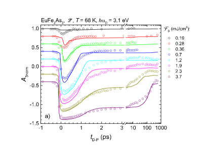
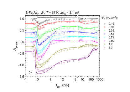
?figurename? 13: (Color online) Comparison of the experimental and simulated trajectories for the case of $\eta=0.01$ and $\phi=\pi/2$. The trajectories at different $\mathcal{F}_{\mathrm{D}}$ are vertically shifted for clarity.

	$\eta$	$\gamma_{\mathrm{e}}$	$G_{\mathrm{eo}}$	$\lambda\left\langle\omega^{2}\right\rangle$	$c_{\mathrm{E}0}$	$G_{\mathrm{ol}}$	$k=\kappa/V_{\mathrm{mol}}$	$L_{\mathrm{D}}/\mathcal{F}_{\mathrm{D}}$
	-	mJ/mol K2	TW/mol K	(meV)2	J/mol K	TW/mol K	W/m K	nm cm2/mJ
Eu-122 (TR-ARPES)Rettig et al. (2013) ($T\sim 100$ K)	$0.01$	$52\pm 3$	$34\pm 3$	$39\pm 3$	$67\pm 14$	$7\pm 5$	-	17
	0.5	$30\pm 2$	$23\pm 3$	$45\pm 3$	$76\pm 20$	$11\pm 9$	-	17
Eu-122 (present work) ($T\sim 70$ K)	0.01	$42\pm 2$	$96\pm 6$	$135\pm 7$	$15\pm 1$	Fig. 14	$14\pm 1$	$17\pm 5$
	0.5	$10\pm 1$	$138\pm 6$	$820\pm 130$	$21\pm 1$
Sr-122 (present work) ($T\sim 70$ K)	0.01	$68\pm 4$	$112\pm 6$	$97\pm 6$	$17\pm 1$	Fig. 14	$10\pm 1$	$23\pm 5$
	0.5	$38\pm 1$	$218\pm 16$	$340\mbox{$\pm$20}$	$25\pm 1$

?tablename? 3: Comparison of the three temperature model parameters obtained from fits with $\mathcal{F}_{\mathrm{D}}$-dependent $G_{\mathrm{ol}}$.

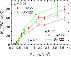
?figurename? 14: (Color online) The destruction-pulse fluence dependence of the electron - optical-phonons coupling from the 3T model fit for two different fixed branching factors.