DyLink2Vec: Effective Feature Representation for
Link Prediction in Dynamic Networks

Abstract

The temporal dynamics of a complex system such as a social network or a communication network can be studied by understanding the patterns of link appearance and disappearance over time. A critical task along this understanding is to predict the link state of the network at a future time given a collection of link states at earlier time points. In existing literature, this task is known as link prediction in dynamic networks. Solving this task is more difficult than its counterpart in static networks because an effective feature representation of node-pair instances for the case of dynamic network is hard to obtain. To overcome this problem, we propose a novel method for metric embedding of node-pair instances of a dynamic network. The proposed method models the metric embedding task as an optimal coding problem where the objective is to minimize the reconstruction error, and it solves this optimization task using a gradient descent method. We validate the effectiveness of the learned feature representation by utilizing it for link prediction in various real-life dynamic networks. Specifically, we show that our proposed link prediction model, which uses the extracted feature representation for the training instances, outperforms several existing methods that use well-known link prediction features.

1 Introduction

Understanding the dynamics of an evolving network is an important research problem with numerous applications in various fields, including social network analysis Otte:2002 , information retrieval jansen:2010 , recommendation systems Ricci:2010 , and bioinformatics jacobs:2001 . A key task towards this understanding is to predict the likelihood of a future association between a pair of nodes, having the knowledge about the current state of the network. This task is commonly known as the link prediction problem. Since, its formal introduction to the data mining community by Liben-Nowell et al. Liben.Nowell:2007 about a decade ago, this problem has been studied extensively by many researchers from a diverse set of disciplines Miller.Jordan.ea:09 ; Ben:2003 ; Lichtenwalter:2010 ; Barbieri:2014 . Good surveys Hasan:2011 ; Wang:2015 on link prediction methods are available for interested readers.

The majority of the existing works on link prediction consider a static snapshot of the given network, which is the state of the networks at a given time Miller.Jordan.ea:09 ; Lichtenwalter:2010 ; Liben.Nowell:2007 ; Menon:2011 . Nevertheless, for many networks, additional temporal information such as the time of link creation and deletion is available over a time interval; for example, in an on-line social or a professional network, we usually know the time when two persons have become friends; for collaboration events, such as, a group performance or a collaborative academic work, we can extract the time of the event from an event calendar. The networks built from such data can be represented by a dynamic network, which is a collection of temporal snapshots of the network. The link prediction task on such a network is defined as follows: for a given pair of nodes, predict the link probability between the pair at time $t+1$ by training the model on the link information at times $1,2,\cdots,t$.

Figure 1: A Toy Dynamic Network. $G_{1}$, $G_{2}$ and $G_{3}$ are three snapshots of the Network. $G_{123}$ is constructed by superimposing $G_{1}$, $G_{2}$ and $G_{3}$.

Link prediction methods for static networks fail to take advantage of the temporal link formation patterns that are manifested by the sequence of multiple temporal snapshots. For illustration, let us consider a toy dynamic network having three temporal snapshots $G_{1}$, $G_{2}$ and $G_{3}$ (see Figure 1). A static link prediction which only considers the latest time stamp $G_{3}$ forfeits the temporal signals that are available from prior snapshots $G_{1}$ and $G_{2}$. Thus, it is oblivious of the fact that the edge $(4,5)$ once existed. On the other hand, if the static link prediction method runs on a superposition Lichtenwalter:2010 of all the available snapshots ($G_{123}$), it fails to preserve the temporal variation in the dataset. For example, the superimposed static snapshot fails to distinguish the link strength between the edges $(3,5)$ and $(4,5)$—even though both edges appear twice in $G_{1}$, $G_{2}$ and $G_{3}$, the recency of $(3,5)$ may make it more likely to re-appear than $(4,5)$.

A key challenge of link prediction in a dynamic setting is to find a suitable feature representation of the node-pair instances which are used for training the prediction model. For the static setting, various topological metrics (common neighbors, Adamic-Adar, Jaccard’s coefficient) are used as features, but they cannot be extended easily for the dynamic setting having multiple snapshots of the network. In fact, when multiple (say $t$) temporal snapshots of a network are provided, each of these scalar features becomes a $t$-size sequence. Flattening the sequence into a $t$-size vector distorts the inherent temporal order of the features. Güneş et al. Gunes2015 overcome this issue by modeling a collection of time series, each for one of the topological features. But such a model fails to capture signals from the neighborhood topology of the edges. There exist few other works on dynamic link prediction, which use probabilistic (non-parametric) and matrix factorization based models. These works consider a feature representation of the nodes and assume that having a link from one node to another is determined by the combined effect of all pairwise node feature interactions ICML2012Sarkar_828 ; KevinS:2013 ; Dunlavy:2011 . While this is a reasonable assumption to make, the accuracy of such models are highly dependent on the quality and availability of the node features, as well as the validity of the above assumption.

There exist a growing list of recent works which use unsupervised methodologies for finding metric embedding of nodes in a graph Perozzi:2014 ; Cao.Lu:15 ; Tang.Qu:15 . The main idea of such methods is to discover latent dependency among the graph vertices and find metric embedding of vertices that captures those relationships. The majority of these works use training methods inspired from neural-network language modeling, such as skip-gram with negative sampling. However, no such work exists for finding feature representation of node-pair instances for the purpose of link prediction in a dynamic network.

In this work, we propose DyLink2Vec, a novel learning method for obtaining a feature representation of node-pair instances, which is specifically suitable for the task of link prediction in a dynamic network. DyLink2Vec  considers the feature learning task as an optimal coding problem, such that the optimal code of a node-pair is the desired feature representation. The learning process can be considered as a two-step compression-reconstruction step, where the first step compresses the input representation of a node-pair into a code by a non-linear transformation, and the second step reconstructs the input representation from the code by a reverse process and the optimal code is the one which yields the least amount of reconstruction error. The input representation of a node-pair is constructed using the connection history and the neighborhood information of the corresponding nodes (details in Section 4). After obtaining an appropriate feature representation of the node-pairs, a standard supervised learning technique can be used (we use AdaBoost) for predicting link states at future times in the given dynamic network.

Below we summarize our contributions in this work:

• We propose a method (DyLink2Vec) for finding metric embedding of node-pairs for the task of link prediction over a dynamic network.

• We validate the effectiveness of DyLink2Vec node-pair embedding by utilizing it for link prediction on four real-life dynamic networks.

• We compare the performance of DyLink2Vec embedding based dynamic link prediction model with multiple state-of-the-art methods. Our comparison results show that the proposed method is significantly superior than all the competing methods.

The paper is organized as follows. In Section 2 we discuss related work. Section 3 defines the problem. In Section 4 we discuss the proposed learning method DyLink2Vec. In Section 5 we detail the link prediction method using DyLink2Vec. Section 6 presents the experimental results to validate the effectiveness of our method. Finally, Section 7 concludes the paper.

2 Related Works

In recent years, the link prediction problem has been studied using a multitude of methodologies. The earliest link prediction methodologies use topological features in a supervised classification setting Hasan06linkprediction ; Liben.Nowell:2007 . More recent methodologies use matrix factorization based approach Menon:2011 . Such methodologies learn latent node representation and predict link strength by the dot product of the latent vectors of corresponding nodes. The objective function of these methods may contain appropriate penalty terms for regularization, and also terms for explicit node and edge features (if available). Recently, Bayesian nonparametric latent feature models have also been proposed for link prediction Miller.Jordan.ea:09 . Unfortunately, all the above methods fail to capture the temporal evolution of the network on a dynamic network setting.

A few methods have been developed for link prediction on dynamic networks. The method proposed by Güneş et al. Gunes2015 capture temporal patterns in a dynamic network using a collection of time-series on topological features. But this approach fails to capture signals from neighborhood topology, as each time-series model is trained on a separate $t$-size feature sequence of a node-pair. Matrix and tensor factorization based solutions are presented in Dunlavy:2011 . Given a three dimensional tensor representation of a dynamic network, the proposed methods use CANDECOMP/PARAFAC (CP) decomposition to capture structural and temporal patterns in the dynamic network. We observe that these methods work well for smaller network, but their prediction performance becomes worse as the network grow larger.

The nonparametric link prediction method presented in ICML2012Sarkar_828 uses features of the node-pairs, as well as the local neighborhood of node-pairs. This method works by choosing a probabilistic model based on features (common neighbor and last time of linkage) of node-pairs. Stochastic block model based approaches KevinS:2013 ; KevinS:2015 divide nodes in a network into several groups and generates edges with probabilities dependent on the group membership of participant nodes. While probabilistic model based link prediction performs well on small networks, they become computationally prohibitive for large networks. A deep learning based solution proposed by Li et al. Li:2014 uses a collection of Restricted Boltzmann Machines with neighbor influence for link prediction in dynamic networks. Tylenda et al. Tylenda:2009 proposed time-aware link prediction method for evolving social networks with hyper-edges.

3 Problem Definition

Let $G(V,E)$ be an undirected network, where $V$ is the set of nodes and $E$ is the set of edges $e(u,v)$ such that $u,v\in V$. A dynamic network is represented as a sequence of snapshots $\mathbb{G}=\{G_{1},G_{2},\dots,G_{t}\}$, where $t$ is the number of time stamps for which we have network snapshots and $G_{i}(V_{i},E_{i})$ is a network snapshot at time stamp $i:1\leq i\leq t$. In this work, we assume that the vertex set remains the same across different snapshots, i.e., $V_{1}=V_{2}=\dots=V_{t}=V$. However, the edges appear and disappear over different time stamps. We also assume that, in addition to the link information, no other attribute data for the nodes or edges are available.

Adjacency matrix representation of a network snapshot $G_{i}$ is represented by a symmetric binary matrix $\mathbf{A}_{i}(n\times n)$, where $n$ is the number of vertices in $G_{i}$. For two vertices $u$ and $v$, $\mathbf{A}_{i}(u,v)=\mathbf{A}_{i}(v,u)=1$, if an edge exists between them in $G_{i}$, and $0$ otherwise. The adjacency vector of a node $u$ at snapshot $G_{i}$ is a $1\times n$ row vector defined as $\mathbf{a}_{i}^{u}=\mathbf{A}_{i}(u,1:n)$.

Problem Statement: Given a sequence of snapshots $\mathbb{G}=\{G_{1},G_{2},\dots,G_{t}\}$ of a network, the task of metric embedding of the node-pairs $(u,v)$ is to obtain a vector $\mathbf{\alpha}^{uv}\in\mathbb{R}^{l}$ ($l$ is the dimensionality of embedding) such that node-pairs having similar local structures across different time snapshots are packed together in the embedding. Once such metric embedding of a node-pair $(u,v)$ is obtained, we use it as the feature representation of this node-pair while predicting the link status between $u$ and $v$ in $G_{t+1}$. Note that, we assume that no link information regarding the snapshot $G_{t+1}$ is available, except the fact that $G_{t+1}$ contains the identical set of vertices.

4 Metric Embedding of Node-Pairs

A key challenge for dynamic link prediction is choosing an effective metric embedding for a given node-pair. Earlier works construct feature vector by adapting various topological similarity metrics for static link prediction or by considering the feature values of different snapshots as a time-series. DyLink2Vec, on the other hand, learns the feature embedding of the node-pairs by using an optimization framework, considering both network topology and link history. Assume a node-pair $(u,v)$ for which we are computing the metric embedding $\mathbf{\alpha}^{uv}\in\mathbb{R}^{d}$. Since we want $\mathbf{\alpha}^{uv}$ to facilitate link prediction on dynamic graphs, the vector $\mathbf{\alpha}^{uv}$ must capture two aspects that influence the possibility of link between $u$ and $v$ in $G_{t+1}$. The first aspect is the similarity between $u$ and $v$ in terms of graph topology across different timestamps, and the second aspect is the history of collaboration between $u$ and $v$—both in the graph snapshots $G_{1},\cdots,G_{t}$.

Consideration of first aspect requires to impart topological similarity signals between $u$ and $v$ into the desired embedded vector $\mathbf{\alpha}^{uv}$ by considering $u$ and $v$’s relation across all the timestamps. To fulfill this objective, we start with a feature vector, $\mathbf{a}^{uv}_{[1,t]}$ of size $nt$ for a node pair $(u,v)$ by taking the element-wise summation of adjacency vectors of $u$ and $v$ over all the timestamps. Thus, for a snapshot $G_{i}$, the adjacency summation vector is $\mathbf{a}_{i}^{uv}=\mathbf{a}_{i}^{u}+\mathbf{a}_{i}^{v}$, and the entire feature vector is the concatenation of $\mathbf{a}_{i}^{uv}$’s from a continuous set of network snapshots, i.e., $\mathbf{a}^{uv}_{[1,t]}=\mathbf{a}_{1}^{uv}~{}||~{}\mathbf{a}_{2}^{uv}~{}||~{}\dots~{}||~{}\mathbf{a}_{t}^{uv}$. Here, the symbol $||$ represents concatenation of two horizontal vectors ( e.g., $0~{}1~{}0~{}||~{}0.5~{}0~{}1=0~{}1~{}0~{}0.5~{}0~{}1$ ).

Figure 2: A toy dynamic network $\mathbb{G}$ with four snapshots $G_{1}$, $G_{2}$ , $G_{3}$ and $G_{4}$. Note that the number of nodes remains constant ($6$) even though the links (edges) may change over time.

Figure 3: (a) Adjacency matrix $\mathbf{A}_{1}$. Each row represents adjacency vector of the corresponding node (b) Computation of node-pair adjacency vector $\mathbf{a}_{1}^{23}$ and $\mathbf{a}_{1}^{45}$.

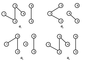
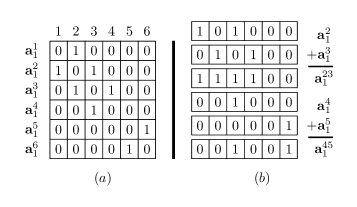
Example: Consider the toy dynamic network shown in Figure 2. The dynamic network $\mathbb{G}=\{G_{1},G_{2},G_{3},G_{4}\}$ has four snapshots. The task is to predict the edges in snap $G_{5}$ (not shown in this figure). The set of nodes does not change over time $(V_{1}=V_{2}=\cdots=V_{5})$. In Figure 3(a) we show the adjacency matrix of the dynamic network $\mathbb{G}$ at time-stamp 1. In Figure 3(b), we show the computation of adjacency vectors of two node-pairs, namely $\mathbf{a}_{1}^{23}$ and $\mathbf{a}_{1}^{45}$. ∎.

The second aspect, history of collaboration between a node-pair is captured by taking cumulative sum of link history, weighted by a time decay function.

$$\mathbf{wclh}^{uv}_{[1,t]}=CumSum(\mathbf{wlh}^{uv}_{[1,t]})$$

Here $\mathbf{wlh}^{uv}_{[1,t]}=w_{1}\cdot\mathbf{A}_{1}(u,v)~{}||~{}w_{2}\cdot\mathbf{A}_{2}(u,v)~{}||~{}\dots~{}||~{}w_{t}\cdot\mathbf{A}_{t}(u,v)$ and $w_{i}=i/t$ is the time decay function. Time decay function $w_{i}$ prioritize more recent linkage information, while cumulative sum rewards reappearance of links (between $u$ and $v$) over different time snapshots.

Finally, the feature vector for a node-pair ($u,v$), $\mathbf{e}^{uv}$, is the concatenation of $\mathbf{a}^{uv}_{[1,t]}$ and ($\mathbf{wclh}^{uv}_{[1,t]}$); i.e., $\mathbf{e}^{uv}=\mathbf{a}^{uv}_{[1,t]}~{}||\mathbf{wclh}^{uv}_{[1,t]}$. DyLink2Vec’s optimization framework converts $\mathbf{e}^{uv}$ to the optimal feature representation $\mathbf{\alpha}^{uv}$ by using a non-linear transformation function $h$ discussed in Section 4.1. Note that, through $h$, the proposed method models complex functions of the entries in $\mathbf{e}^{uv}$, which makes the embedded feature vector $\mathbf{\alpha}^{uv}$ very effective for link prediction in dynamic network.

Our proposed method is different—both, in methodologies and also in objective— from the existing works Tang.Qu:15 ; Perozzi:2014 which construct metric embedding of the vertices of a network. Existing works find embedding of a vertex from a static network, whereas we find embedding of a node-pair from a dynamic network. The learning method of the existing works follow language model, whereas our method follows a compression-reconstruction framework which preserves higher-order neighborhood and link history patterns of the node-pair in its embedded representation. Below we discuss the compression-reconstruction framework which yields the optimal metric embedding through a principled approach.

4.1 Optimization framework for DyLink to Vec

In this section, we discuss the optimization framework which obtains the optimal metric embedding of a node pair by learning an optimal coding function $h$. For this learning task, let’s assume $\mathbf{\widehat{E}}$ is the training dataset matrix containing a collection of node-pair feature vectors. Each row of this matrix represents a node-pair (say, $u$ and $v$) and it contains the feature vector $\mathbf{e}^{uv}$ which stores information about neighborhood and link history, as we discussed earlier. The actual link status of the node-pairs in $\mathbf{\widehat{E}}$ in $G_{t+1}$ is not used for the learning of $h$, so the metric embedding process is unsupervised. In subsequent discussion, we write $\mathbf{e}$ to represent an arbitrary node pair vector in $\mathbf{\widehat{E}}$.

Now, the coding function $h$ compresses $\mathbf{e}$ to a code vector $\mathbf{\alpha}$ of dimension $l$, such that $l<k$. Here $l$ is a user-defined parameter which represents the code length and $k$ is the size of feature vector. Many different coding functions exist in the dimensionality reduction literature, but for DyLink2Vec we choose the coding function which incurs the minimum reconstruction error in the sense that from the code $\mathbf{\alpha}$ we can reconstruct $\mathbf{e}$ with the minimum error over all $\mathbf{e}\in\mathbf{\widehat{E}}$. We frame the learning of $h$ as an optimization problem, which we discuss below through two operations: Compression and Reconstruction.

Compression: It obtains $\mathbf{\alpha}$ from $\mathbf{e}$. This transformation can be expressed as a nonlinear function of linear weighted sum of the entries in vector $\mathbf{e}$.

$$\mathbf{\alpha}=f(\mathbf{W}^{(c)}\mathbf{e}+\mathbf{b}^{(c)})$$ (1)

$\mathbf{W}^{(c)}$ is a $(k\times l)$ dimensional matrix. It represents the weight matrix for compression and $\mathbf{b}^{(c)}$ represents biases. $f(\cdot)$ is the Sigmoid function, $f(x)=\frac{1}{1+e^{-x}}$.

Reconstruction: It performs the reverse operation of compression, i.e., it obtains $\mathbf{e}$ from $\mathbf{\alpha}$ (which was constructed during the compression operation).

$$\mathbf{\beta}=f(\mathbf{W}^{(r)}\mathbf{\alpha}+\mathbf{b}^{(r)})$$ (2)

$\mathbf{W}^{(r)}$ is a matrix of dimensions $(l\times k)$ representing the weight matrix for reconstruction, and $\mathbf{b}^{(r)}$ represents biases.

The optimal coding function $h$ constituted by the compression and reconstruction operations is defined by the parameters $(\mathbf{W},\mathbf{b})=(\mathbf{W}^{(c)},\mathbf{b}^{(c)},\mathbf{W}^{(r)},\mathbf{b}^{(r)})$. The objective is to minimize the reconstruction error. Reconstruction error for a neighborhood based feature vector $\mathbf{(}e)$ is defined as, $J(\mathbf{W,b,e})=\frac{1}{2}\parallel\mathbf{\beta}-\mathbf{e}\parallel^{2}$. Over all possible feature vectors, the average reconstruction error augmented with a regularization term yields the final objective function $J(\mathbf{W},\mathbf{b})$:

$$\begin{split}J(\mathbf{W},\mathbf{b})=\frac{1}{{|\mathbf{\widehat{E}}|}}\sum_{\mathbf{e}\in\mathbf{\widehat{E}}}(\frac{1}{2}\parallel\mathbf{\beta}^{uv}-\mathbf{e}^{uv}\parallel^{2})\\ +\frac{\lambda}{2}(\parallel\mathbf{W}^{(c)}\parallel_{F}^{2}+\parallel\mathbf{W}^{(r)}\parallel_{F}^{2})\end{split}$$ (3)

Here, $\lambda$ is a user assigned regularization parameter, responsible for preventing over-fitting. $\parallel\cdot\parallel_{F}$ represents the Frobenius norm of a matrix. In this work we use $\lambda=0.1$.

To this end, we discuss the motivation of our proposed optimization framework for learning the coding function $h$. Note that, the dimensionality of $\mathbf{\alpha}$ is much smaller than $\mathbf{e}$, so the optimal compression of the vector $\mathbf{e}$ must extract patterns composing of the entries of $\mathbf{e}$ and use them as high-order latent feature in $\mathbf{\alpha}$. In fact, the entries in $\mathbf{e}$ contain the neighborhood (sum of adjacency vector of the node pair) and link history of a node-pair for all the timestamps; for a real-life network, this vector is sparse and substantial compression is possible incurring small loss. Through this compression the coding function $h$ learns the patterns that are similar across different node-pairs (used in $\mathbf{\widehat{E}}$). Thus the function $h$ learns a metric embedding of the node-pairs that packs node-pairs having similar local structures in close proximity in the embedded feature space. Although function $h$ acts as a black-box, it captures patterns involving neighborhood around a node pair across various time stamps, which obviates the manual construction of a node-pair feature—a cumbersome task for the case of a dynamic network.

4.1.1 Optimization

The training of optimal coding defined by parameters $(\mathbf{W,b})$ begins with random initialization of the parameters. Since the cost function $J(\mathbf{W},\mathbf{b})$ defined in Equation (3) is non-convex in nature, we obtain a local optimal solution using the gradient descent approach. Such approach usually provides practically useful results (as shown in the Section 6). The parameter updates of the gradient descent are similar to the parameter updates for optimizing Auto-encoder in machine learning. One iteration of gradient descent updates the parameters using following equations:

$$\begin{split}W_{ij}^{(c)}=W_{ij}^{(c)}-\sigma\frac{\partial}{\partial W_{ij}^{(c)}}J(W,b)\\ W_{ij}^{(r)}=W_{ij}^{(r)}-\sigma\frac{\partial}{\partial W_{ij}^{(r)}}J(W,b)\\ b_{i}^{(c)}=b_{i}^{(c)}-\sigma\frac{\partial}{\partial b_{i}^{(c)}}J(W,b)\\ b_{i}^{(r)}=b_{i}^{(r)}-\sigma\frac{\partial}{\partial b_{i}^{(r)}}J(W,b)\end{split}$$ (4)

Here, $l$ appropriately identifies the weight and bias parameters $l\in\{1,2\}$. $\sigma$ is the learning rate. $W_{ij}^{(1)}$ is the weight of connection between node $j$ of the input layer to node $i$ of the hidden layer.

Now, from Equation (3), the partial derivative terms in equations (4) can be written as,

$$\begin{split}\frac{\partial}{\partial W_{ij}^{(c)}}J(W,b)=\frac{1}{|\mathbf{\widehat{E}}|}\sum_{\mathbf{e}\in\mathbf{\widehat{E}}}\frac{\partial}{\partial W_{ij}^{(c)}}J(\mathbf{W,b,e})+\lambda W_{ij}^{(c)}\\ \frac{\partial}{\partial W_{ij}^{(r)}}J(W,b)=\frac{1}{|\mathbf{\widehat{E}}|}\sum_{\mathbf{e}\in\mathbf{\widehat{E}}}\frac{\partial}{\partial W_{ij}^{(r)}}J(\mathbf{W,b,e})+\lambda W_{ij}^{(r)}\\ \frac{\partial}{\partial b_{i}^{(c)}}J(W,b)=\frac{1}{|\mathbf{\widehat{E}}|}\sum_{\mathbf{e}\in\mathbf{\widehat{E}}}\frac{\partial}{\partial b_{i}^{(c)}}J(\mathbf{W,b,e})\\ \frac{\partial}{\partial b_{i}^{(r)}}J(W,b)=\frac{1}{|\mathbf{\widehat{E}}|}\sum_{\mathbf{e}\in\mathbf{\widehat{E}}}\frac{\partial}{\partial b_{i}^{(r)}}J(\mathbf{W,b,e})\\ \end{split}$$ (5)

The optimization problem is solved by computing partial derivative of cost function $J(\mathbf{W,b,e})$ using the back propagation approach Rumelhart:1986 .

Once the optimization is done, the metric embedding of any node-pair ($u,v$) can be obtained by taking the outputs of compression stage (Equation (1)) of the trained optimal coding ($\mathbf{W,b}$).

$$\begin{split}\mathbf{\alpha}^{uv}=f(\mathbf{W}^{(c)}\mathbf{e}^{uv}+\mathbf{b}^{(c)})=h(\mathbf{e}^{uv})\end{split}$$ (6)

4.1.2 Complexity Analysis

We use Matlab implementation of optimization algorithm L-BFGS (Limited-memory Broyden-Fletcher-Goldfarb-Shanno) for learning optimal coding. We execute the algorithm for a limited number of iterations to obtain unsupervised features within a reasonable period of time. Each iteration of L-BFGS executes two tasks for each node-pair: back-propagation to compute partial differentiation of cost function, and change the parameters $\mathbf{(W,b)}$. Therefore, the time complexity of one iteration is $O(|NP_{t}|kl)$. Here, $NP_{t}$ is the set on node-pairs used to construct the training dataset $\mathbf{\widehat{E}}$. $k$ is the length of $\mathbf{e}$ (dimensionality of initial edge features), and $l$ is length of $\mathbf{\alpha}$ (optimal coding).

5 Link Prediction using proposed metric embedding

For link prediction task in a dynamic network, $\mathbb{G}=\{G_{1},G_{2},\dots,G_{t}\}$; we split the snapshots into two overlapping time windows, $[1,t-1]$ and $[2,t]$. Training dataset, $\mathbf{\widehat{E}}$ is feature representation for time snapshots $[1,t-1]$, the ground truth ($\widehat{\mathbf{y}}$) is constructed from $G_{t}$. DyLink2Vec learns optimal embedding $h(\cdot)$ using training dataset $\mathbf{\widehat{E}}$. After training a supervised classification model using $\widehat{\mathbf{\alpha}}$=$h(\widehat{\mathbf{E}})$ and $\widehat{\mathbf{y}}$, prediction dataset $\mathbf{\overline{E}}$ is used to predict links at $G_{t+1}$. For this supervised prediction task, we experiment with several classification algorithms. Among them SVM (support vector machine) and AdaBoost perform the best.

1:procedure LPDyLink2Vec($\mathbb{G},t$) Input: $\mathbb{G}$: Dynamic Network, $t$: Time steps

Output: $\overline{y}$: Forecasted links at time step $t+1$

1

2:     $\widehat{\mathbf{E}}$=NeighborhoodFeature($\mathbb{G}$,$1$,$t-1$)

3:     $\widehat{\mathbf{y}}$=Connectivity($G_{t}$)

4:     $\overline{\mathbf{E}}$=NeighborhoodFeature($\mathbb{G}$,$2$,$t$)

5:     $h$=LearningOptimalCoding($\widehat{\mathbf{E}}$)

6:     $\widehat{\mathbf{\alpha}}$=$h(\widehat{\mathbf{E}})$

7:     $\overline{\mathbf{\alpha}}$=$h(\overline{\mathbf{E}})$

8:     $C$=TrainClassifier($\widehat{\mathbf{\alpha}},\widehat{\mathbf{y}}$)

9:     $\overline{\mathbf{y}}$=LinkForecasting($C,\overline{\mathbf{\alpha}}$)

10:     return $\overline{\mathbf{y}}$

11:end procedure

Algorithm 1 Link Prediction using DyLink2Vec

The pseudo-code of DyLink2Vec based link prediction method is given in Algorithm 1. For training link prediction model, we split the available network snapshots into two overlapping time windows, $[1,t-1]$ and $[2,t]$. Neighborhood based features $\widehat{\mathbf{E}}$ and $\overline{\mathbf{E}}$ are constructed in Lines 2 and 4, respectively. Then we learn optimal coding for node-pairs using neighborhood features $\widehat{\mathbf{E}}$ (in Line 5). Embeddings are constructed using learned optimal coding (Lines 6 and 7) using output of compression stage (Equation 6). Finally, a classification model $C$ is learned (Line 8), which is used for predicting links in $G_{t+1}$ (Line 9).

6 Experiments and Results

We demonstrate the performance of DyLink2Vec using four real world dynamic network datasets: Enron, Collaboration, Facebook1 and Facebook2. We show performance comparison between DyLink2Vec based link prediction method and existing state-of-the-art dynamic link prediction methodologies. Experimental results also include the discussion of DyLink2Vec’s performance for varying length of time stamps in the network, and varying degree of class imbalance in training dataset. Bellow, we discuss the datasets, evaluation metrics, competing methods, implementation details and results.

(a) Enron Network

(b) Enron Network

(c) Collaboration Network

(d) Collaboration Network

(e) Facebook1 Network

(f) Facebook1 Network

(g) Facebook2 Network

(h) Facebook2 Network

Figure 4: Comparison with competing link prediction methods. Each bar represents a methods and the height of the bar represents the value of the performance metrics. Results for Enron network are presented in charts (a)-(b), results of Collaboration data are presented in charts (c)-(d), the results of Facebook1 data are in charts (e)-(f), and the results of Facebook2 data are in charts (g)-(h). The group of bars in a chart are distinguished by color, so the figure is best viewed on a computer screen or color print.

6.1 Dataset Descriptions

Here we discuss the construction and characteristics of the datasets used for experiments.

Enron email corpus priebe2005scan consists of email exchanges between Enron employees. The Enron dataset has $11$ time stamps and $16,836$ possible node-pairs; the task is to use first $10$ snapshots for predicting links in the $11^{th}$ snapshot. Following KevinS:2013 , we aggregate data into time steps of $1$ week. We use the data from weeks $147$ to $157$ of the data trace for the experiments. The reason for choosing that window is that the snapshot of the graph at week $157$ has the highest number of edges.

Collaboration dataset has $10$ time stamps with author collaboration information about $49,455$ author-pairs. The Collaboration dataset is constructed from citation data containing $1.4$ million papers Tang:2008 . We process the data to construct a network of authors with edges between them if they co-author a paper. Considering each year as a time stamp, the data of years $2000$-$2009$ ($10$ time stamps) is used for this experiment, where the data from the first nine time stamps is used for training and the last for prediction. Since this data is very sparse, we pre-process the data to retain only the active authors, who have last published papers on or after year $2010$; moreover, the selected authors participate in at least two edges in seven or more time stamps.

Facebook1 and Facebook2 are network of Facebook wall posts viswanath2009evolution . Each vertex is a Facebook user account and an edge represents the event that one user posts a message on the wall of another user. Both Facebook1 and Facebook2 has $9$ time stamps. Facebook1 has $219,453$ node-pairs. Facebook2 is an extended version of Facebook1 dataset with $883,785$ node-pairs. For pre-processing Facebook1 we follow the same setup as is discussed in KevinS:2015 ; wall posts of 90 days are aggregated in one time step.

We filter out all people who are active for less than 6 of the 9 time steps, along with the people who have degree less than 30. Facebook2 is created using a similar method, but a larger sample of Facebook wall posts is used for this dataset.

6.2 Evaluation Metrics

For evaluating the proposed method we use two metrics, namely, area under Precision-Recall (PR) curve (PRAUC) Davis:2006 and an information retrieval metric, Normalized Discounted Cumulative Gain (NDCG). PRAUC is best suited for evaluating two class classification performance when class membership is skewed towards one of the classes. This is exactly the case for link prediction; the number of edges $(|E|)$ is very small compared to the number of possible node-pairs ${|V|\choose 2}$ In such scenarios, area under the Precision-Recall curve (PRAUC) gives a more informative assessment of the algorithm’s performance than other metrics such as, accuracy. The reason why PRAUC is more suitable for the skewed problem is that it does not factor in the count of true negatives in its calculation. In skewed data where the number of negative examples is huge compared to the number of positive examples, true negatives are not that meaningful.

We also use NDCG, an information retrieval metric (widely used by the recommender systems community) to evaluate the proposed method. NDCG measures the performance of link prediction system based on the graded relevance of the recommended links. $NDCG_{k}$ varies from 0.0 to 1.0, with 1.0 representing ideal ranking of edges. Here, $k$ is a parameter chosen by user representing the number of links ranked by the method. We use $k=50$ in all our experiments.

Some of the earlier works on link prediction have used area under the ROC curve (AUC) to evaluate link prediction works Gunes2015 ; Wang:2007 . But recent works Yang2015 have demonstrated the limitations of AUC and argued in favor of PRAUC over AUC for evaluation of link prediction. So we have not used AUC in this work.

6.3 Competing Methods for Comparison

We compare the performance of DyLink2Vec based link prediction method with methods from four categories: (1) topological feature based methods, (2) feature time series based methods Gunes2015 , (3) a deep learning based method, namely DeepWalk Perozzi:2014 , and (4) a tensor factorization based method CANDECOMP/PARAFAC (CP) Dunlavy:2011 .

Besides these four works, there are two other existing works for link prediction in dynamic network setting; one is based on deep Learning Li:2014 (Conditional Temporal Restricted Boltzmann machine) and the other is based on a signature-based nonparametric method ICML2012Sarkar_828 . We did not compare with these models as implementations of their models are not readily available, besides, both of these methods have numerous parameters which will make reproducibility of their results highly improbable and thus, conclusion derived from such experiments may not align with true understanding of the usefulness of the methods. Moreover, none of these methods give unsupervised feature representation for node-pairs in which we claim our main contribution.

For topological feature based methods, we consider four prominent topological features: Common Neighbors ($CN$), Adamic-Adar ($AA$), Jaccard’s Coefficient ($J$) and Katz measure ($Katz$). However, in existing works, these features are defined for static networks only; so we adapt these features for the dynamic network setting by computing the feature values over the collapsed dynamic network.

We also combine the above four features to construct a combined feature vector of length four (Jaccard’s Coefficient, Adamic-Adar, Common Neighbors and Katz), which we call $JACK$ and use it with a classifier to build a supervised link prediction method, and include this model in our comparison.

Second, we compare DyLink2Vec with time-series based neighborhood similarity scores proposed in Gunes2015 . In this work, the authors consider several neighborhood-based node similarity scores combined with connectivity information (historical edge information). Authors use time-series of similarities to model the change of node similarities over time. Among $16$ proposed methods, we consider $4$ that are relevant to the link prediction task on unweighted networks and also have the best performance. $TS\mbox{-}CN\mbox{-}Adj$ represents time-series on normalized score of Common Neighbors and connectivity values at time stamps $[1,t]$. Similarly, we get time-series based scores for Adamic-Adar ($TS\mbox{-}AA\mbox{-}Adj$), Jaccard’s Coefficient ($TS\mbox{-}J\mbox{-}Adj$) and Preferential Attachment ($TS\mbox{-}PA\mbox{-}Adj$).

Third, we compare DyLink2Vec with DeepWalk Perozzi:2014 , a latent node representation based method. We use DeepWalk to construct latent representation of nodes from the collapsed dynamic network. Then we construct latent representation of node-pairs by computing cross product of latent representation of the participating nodes. For example, if the node representations in a network are vectors of size $l$, then the representation of a node-pair $(u,v)$ will be of size $l^{2}$, constructed from the cross product of $u$ and $v$’s representation. The DeepWalk based node-pair representation is then used with a classifier to build a supervised link prediction method. We choose node representation size $l=2,4,6,8,10$ and report the best performance.

Finally, we compare DyLink2Vec with a tensor factorization based method, called CANDECOMP/PARAFAC (CP) Dunlavy:2011 . In this method, the dynamic network is represented as a three-dimensional tensor $\mathcal{Z}(n\times n\times t)$. Using CP decomposition $\mathcal{Z}$ is factorized into three factor matrices. The link prediction score is computed by using the factor matrices. We adapted the CP link prediction method for unipartite networks; which has originally been developed for bipartite networks.

6.4 Implementation Details

We implemented DyLink2Vec algorithm in Matlab version $R2014b$. The learning method runs for a maximum of $100$ iterations or until it converges to a local optimal solution. We use coding size $l=100$ for all datasets. For supervised link prediction step we use several Matlab provided classification algorithms, namely, AdaBoostM1, RobustBoost, and Support Vector Machine (SVM). We could use neural network classifier. But, as our main goal is to evaluate the quality of unsupervised feature representation, so, we use simple classifiers. Supervised neural network architecture may result in superior performance, but, it is out of scope of the main goal of the paper. We use Matlab for computing the feature values (CN, AA, J, Katz) that we use in other competing methods. Time-series methods are implemented using Python. We use the ARIMA (autoregressive integrated moving average) time series model implemented in Python module statsmodels. The DeepWalk implementation is provided by the authors of Perozzi:2014 . We use it to extract node features and extend it for link prediction (using Matlab). Tensor factorization based method CP was implemented using Matlab Tensor Toolbox.

6.5 Performance Comparison Results with Competing Methods

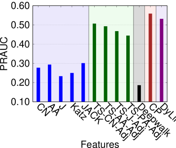
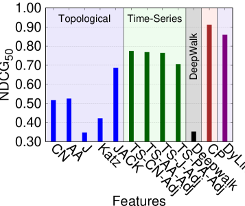
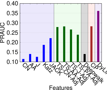
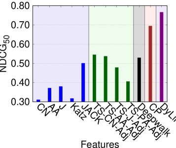
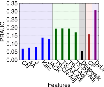
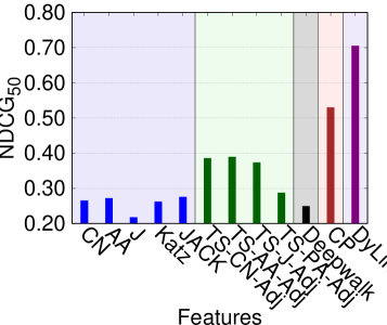
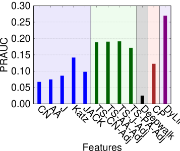
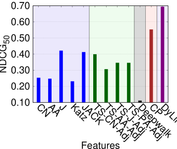
In Figure 4 we present the performance comparison results of DyLink2Vec based link prediction method with the four kinds of competing methods that we have discussed earlier. The figure have eight bar charts. The bar charts from the top to the bottom rows display the results for Enron, Collaboration, Facebook1 and Facebook2 datasets, respectively. The bar charts in a row show comparison results using PRAUC (left), and $NDCG_{50}$ (right) metrics. Each chart has twelve bars, each representing a link prediction method, where the height of a bar is indicative of the performance metric value of the corresponding method. In each chart, from left to right, the first five bars (blue) correspond to the topological feature based methods, the next four (green) represent time series based methods, the tenth bar (black) is for DeepWalk, the eleventh bar (brown) represents tensor factorization based method CP, and the final bar (purple) represents the proposed method DyLink2Vec.

6.5.1 DyLink2Vec vs. Topological

We first analyze the performance comparison between DyLink2Vec based method and topological feature based methods (first five bars). The best of the topological feature based methods have a PRAUC value of 0.30, 0.22, 0.137 and 0.14 in Enron, Collaboration, Facebook1, and Facebook2 dataset (see Figures 4(a), 4(c), 4(e) and 4(g)), whereas the corresponding PRAUC values for DyLink2Vec are 0.531, 0.362, 0.308, and 0.27, which translates to 77%, 65%, 125%, and 93% improvement of PRAUC by DyLink2Vec for these datasets. Superiority of DyLink2Vec over all the topological feature based baseline methods can be attributed to the capability of Neighborhood based feature representation to capture temporal characteristics of local neighborhood. Similar trend is observed using $NDCG_{50}$ metric, see Figures 4(b), 4(d), 4(f) and 4(h).

6.5.2 DyLink2Vec vs. Time-Series

The performance of time-series based method (four green bars) is generally better than the topological feature based methods. The best of the time-series based method has a PRAUC value of 0.503, 0.28, 0.19, and 0.19 on these datasets, and DyLink2Vec’s PRAUC values are better than these values by 6%, 29%, 62%, and 42% respectively. Time-series based methods, though model the temporal behavior well, probably fail to capture signals from the neighborhood topology of the node-pairs. Superiority of DyLink2Vec over Time-Series methods is also similarly indicated by information retrieval metric $NDCG_{50}$.

6.5.3 DyLink2Vec vs. DeepWalk

The DeepWalk based method (black bars in Figure 4) performs much poorly in terms of both PRAUC and $NDCG_{50}$—even poorer than the topological based method in all four datasets. Possible reason could be the following: the latent encoding of nodes by DeepWalk is good for node classification, but the cross-product of those codes fails to encode the information needed for effective link prediction.

6.5.4 DyLink2Vec vs. CANDECOMP/PARAFAC (CP)

Finally, the tensor factorization based method CP performs marginally better (around 5% in PRAUC, and 6% in $NDCG_{50}$) than DyLink2Vec in small and simple networks, such as Enron (see Figure 4(a, b)). But its performance degrades on comparatively large and complex networks, such as Collaboration, Facebook1 and Facebook2. On Facebook networks, the performance of CP is even worse than the time-series based methods (see Figures 4(e) and 4(g)). DyLink2Vec comfortably outperforms CP on larger graphs, see Figures 4(c, d, e, f, g, h). In terms of PRAUC, DyLink2Vec outperforms CP by 28%, 94%, and 120% for Collaborative, Facebook1 and Facebook2 networks respectively. This demonstrates the superiority of DyLink2Vec over one of the best state-of-the-art dynamic link prediction. A reason for CP’s bad performance on large graphs can be its inability to capture network structure and dynamics using high-dimensional tensors representation.

6.5.5 Performance across datasets

When we compare the performance of all the methods across different datasets, we observe varying performance. For example, for both the metrics, the performance of dynamic link prediction on Facebook graphs are lower than the performance on Collaboration graph, which, subsequently, is lower than the performance on Enron graph, indicating that link prediction in Facebook data is a harder problem to solve. In these harder networks, DyLink2Vec perform substantially better than all the other competing methods that we consider in this experiment.

(a) Collaboration Network

(b) Facebook1 Network

Figure 5: Change in link prediction performance with number of time stamps. X-axis represents size of training window used for link prediction. Largest possible window size depends on number of time stamps available for the dataset.

6.6 Performance with varying length of Time Stamps

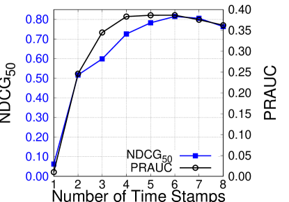
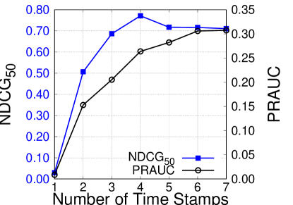
Besides comparing with competing methods, we also demonstrate the performance of DyLink2Vec with varying number of available time snapshots. For this purpose, we use DyLink2Vec with different counts of past snapshots. For example, Collaboration dataset has 10 time stamps. The task is to predict links at time stamp 10. The largest number of past snapshots we can consider for this data is 8, where $\mathbf{\widehat{E}}$ is constructed using time stamps $[1-8]$, and $\mathbf{\overline{E}}$ is constructed using time stamps $[2-9]$. The smallest number of time stamps we can consider is 1, where $\mathbf{\widehat{E}}$ is constructed using $[8-8]$, and $\mathbf{\overline{E}}$ is constructed using $[9-9]$. In this way, by varying the length of historical time stamps, we can evaluate the effect of time stamp’s length on the performance of a link prediction method.

The result is illustrated in Figure 5. The x-axis represents the number of time stamps used by DyLink2Vec, the left y-axis represents the $NDGC_{50}$ and the right y-axis represents the PRAUC. Figures 5(a), and 5(b) corresponds to the results obtained on Collaboration and Facebook1, respectively.

We observe from Figure 5 that the performance ($NDGC_{50}$ and PRAUC) of link prediction increases with increased number of time stamps. But beyond a given number of snapshots, the performance increment becomes insignificant. The performance starts to deteriorate after certain number of snapshots (see Figure 5(a)). This may be because of the added complexity of the optimization framework with increased number of time stamps. We also observe consistent improvement of performance with the number of snapshots for the Facebook1 data (Figure 5(b)), which indicates that for this dataset link information from distant history is useful for dynamic link prediction. We do not show results of Enron and Facebook2 for this experiment, because of space constraint, however, they show similar trends.

Figure 6: Effect of class imbalance in link prediction performance on Collaboration network.

6.7 Effect of Class Imbalance on Performance

In link prediction problem, class imbalance is a prevalent issue. The class imbalance problem appears in a classification task, when the dataset contains imbalanced number of samples for different classes. In link prediction problem, the number of positive node-pairs (with an edge) is very small compared to the number of negative node-pairs (with no edge), causing class imbalance problem.

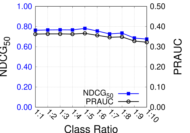
To demonstrate the effect of class imbalance in link prediction task, we perform link prediction using DyLink2Vec embeddings with different level of class imbalance in the training dataset. We construct the training dataset by taking all positive node-pairs and sampling from the set of negative node-pairs. For a balanced dataset, the number of negative samples will be equal to the number of all positive node-pairs considered. Thus, the balanced training dataset has positive node-pairs to negative node-pairs ratio $1:1$. At this point, the only way to increase the size of the data is to increase the sample size for negative node-pairs. Consequently, the ratio of classes also increases towards negative node-pair. Figure 6 shows gradual decrease in link prediction performance in Collaboration network with the increase of imbalance (see ratios in X-axis) in the dataset (despite the fact that the dataset gets larger by adding negative node-pairs).

This result advocates towards the design choice of under-sampling Lichtenwalter:2010 of negative node-pairs by uniformly sampling from all negative node-pairs, so that the training set has equal numbers of positive and negative node-pairs. Under-sampling, helps to mitigate the problem of class imbalance while also reducing the size of the training dataset.

7 Conclusion

In this paper, we present DyLink2Vec a learning method for obtaining feature representation of node-pairs in dynamic networks. We also give classification based link prediction method, which uses DyLink2Vec feature representation for future link prediction in dynamic network setup. The proposed link prediction method outperforms several existing methods that are based on topological features, time series, deep learning and tensor analysis.

References

- (1) Barbieri, N., Bonchi, F., Manco, G.: Who to follow and why: Link prediction with explanations. In: Proceedings of the 20th ACM SIGKDD International Conference on Knowledge Discovery and Data Mining, KDD ’14, pp. 1266–1275 (2014)
- (2) Cao, S., Lu, W., Xu, Q.: Grarep: Learning graph representations with global structural information. In: Proceedings of the 24th ACM International on Conference on Information and Knowledge Management, pp. 891–900. ACM (2015)
- (3) Davis, J., Goadrich, M.: The relationship between precision-recall and roc curves. In: Proceedings of the 23rd International Conference on Machine Learning, ICML ’06, pp. 233–240 (2006)
- (4) Dunlavy, D.M., Kolda, T.G., Acar, E.: Temporal link prediction using matrix and tensor factorizations. ACM Trans. Knowl. Discov. Data 5(2), 10:1–10:27 (2011)
- (5) Güneş, İ., Gündüz-Öğüdücü, Ş., Çataltepe, Z.: Link prediction using time series of neighborhood-based node similarity scores. Data Mining and Knowledge Discovery 30(1), 147–180 (2015)
- (6) Hasan, M., Zaki, M.: A survey of link prediction in social networks. In: C.C. Aggarwal (ed.) Social Network Data Analytics, pp. 243–275 (2011)
- (7) Hasan, M.A., Chaoji, V., Salem, S., Zaki, M.: Link prediction using supervised learning. In: Proc. of SDM 06 workshop on Link Analysis, Counterterrorism and Security (2006)
- (8) Jacobs, D.J., Rader, A.J., Kuhn, L.A., Thorpe, M.F.: Protein flexibility predictions using graph theory. Proteins: Structure, Function, and Bioinformatics 44(2), 150–165 (2001)
- (9) Jansen, B.J., Rieh, S.Y.: The seventeen theoretical constructs of information searching and information retrieval. Journal of the American Society for Info. Science and Technology 61(8), 1517–1534 (2010)
- (10) Li, X., Du, N., Li, H., Li, K., Gao, J., Zhang, A.: A deep learning approach to link prediction in dynamic networks. In: Proc. of the SIAM Intl. Conference on Data Mining, pp. 289–297 (2014)
- (11) Liben-Nowell, D., Kleinberg, J.: The link-prediction problem for social networks. J. Am. Soc. Inf. Sci. Technol. 58(7), 1019–1031 (2007)
- (12) Lichtenwalter, R.N., Lussier, J.T., Chawla, N.V.: New perspectives and methods in link prediction. In: Proceedings of the 16th ACM SIGKDD International Conference on Knowledge Discovery and Data Mining, KDD ’10, pp. 243–252. New York, NY, USA (2010)
- (13) Menon, A.K., Elkan, C.: Link prediction via matrix factorization. In: Proceedings of the 2011 European Conference on Machine Learning and Knowledge Discovery in Databases - Volume Part II, ECML PKDD’11, pp. 437–452 (2011)
- (14) Miller, K., Jordan, M.I., Griffiths, T.L.: Nonparametric latent feature models for link prediction. In: Advances in Neural Information Processing Systems, pp. 1276–1284 (2009)
- (15) Otte, E., Rousseau, R.: Social network analysis: a powerful strategy, also for the information sciences. Journal of Information Science 28(6), 441–453 (2002)
- (16) Perozzi, B., Al-Rfou, R., Skiena, S.: Deepwalk: Online learning of social representations. In: Proceedings of the 20th ACM SIGKDD International Conference on Knowledge Discovery and Data Mining, KDD ’14, pp. 701–710. New York, NY, USA (2014)
- (17) Priebe, C.E., Conroy, J.M., Marchette, D.J., Park, Y.: Scan statistics on enron graphs. Comp. & Math. Organization Theory 11(3), 229–247 (2005)
- (18) Ricci, F., Rokach, L., Shapira, B., Kantor, P.B.: Recommender Systems Handbook, 1st edn. Springer-Verlag New York, Inc., New York, NY, USA (2010)
- (19) Rumelhart, D.E., Hinton, G.E., Williams, R.J.: Parallel distributed processing: Explorations in the microstructure of cognition, vol. 1. chap. Learning Internal Representations by Error Propagation, pp. 318–362 (1986)
- (20) Sarkar, P., Chakrabarti, D., Jordan, M.I.: Nonparametric link prediction in dynamic networks. In: J. Langford, J. Pineau (eds.) Proceedings of the 29th Intl. Conference on Machine Learning (ICML-12), pp. 1687–1694 (2012)
- (21) Tang, J., Qu, M., Wang, M., Zhang, M., Yan, J., Mei, Q.: Line: Large-scale information network embedding. In: Proceedings of the 24th International Conference on World Wide Web, pp. 1067–1077. ACM (2015)
- (22) Tang, J., Zhang, J., Yao, L., Li, J., Zhang, L., Su, Z.: Arnetminer: Extraction and mining of academic social networks. In: Proceedings of the 14th ACM SIGKDD Intl Conference on Knowledge Discovery and Data Mining, KDD ’08, pp. 990–998 (2008)
- (23) Taskar, B., fai Wong, M., Abbeel, P., Koller, D.: Link prediction in relational data. In: Advances in Neural Information Processing Systems 16, pp. 659–666. MIT Press (2004)
- (24) Tylenda, T., Angelova, R., Bedathur, S.: Towards time-aware link prediction in evolving social networks. In: Proceedings of the 3rd Workshop on Social Network Mining and Analysis, pp. 9:1–9:10. ACM (2009)
- (25) Viswanath, B., Mislove, A., Cha, M., Gummadi, K.P.: On the evolution of user interaction in facebook. In: Proceedings of the 2nd ACM workshop on Online social networks, pp. 37–42. ACM (2009)
- (26) Wang, C., Satuluri, V., Parthasarathy, S.: Local probabilistic models for link prediction. In: Proceedings of the 2007 Seventh IEEE International Conference on Data Mining, ICDM ’07, pp. 322–331 (2007)
- (27) Wang, P., Xu, B., Wu, Y., Zhou, X.: Link prediction in social networks: the state-of-the-art. Science China Information Sciences 58(1), 1–38 (2015)
- (28) Xu, K.S.: Stochastic block transition models for dynamic networks. In: Proceedings of the 18th International Conference on Artificial Intelligence and Statistics, pp. 1079–1087 (2015)
- (29) Xu, K.S., Hero III, A.O.: Dynamic stochastic blockmodels for time-evolving social networks. IEEE Journal of Selected Topics in Signal Processing 8(4), 552–562 (2014)
- (30) Yang, Y., Lichtenwalter, R.N., Chawla, N.V.: Evaluating link prediction methods. Knowledge and Information Systems 45(3), 751–782 (2015)