Nitrogen fractionation in high-mass star-forming cores across the Galaxy

Abstract

The fractionation of nitrogen (N) in star-forming regions is a poorly understood process. To put more stringent observational constraints on the N-fractionation, we have observed with the IRAM-30m telescope a large sample of 66 cores in massive star-forming regions. We targeted the (1–0) rotational transition of HN¹³C, HC¹⁵N, H¹³CN and HC¹⁵N, and derived the ¹⁴N/¹⁵N ratio for both HCN and HNC. We have completed this sample with that already observed by Colzi et al. (2018), and thus analysed a total sample of 87 sources. The ¹⁴N/¹⁵N ratios are distributed around the Proto-Solar Nebula value with a lower limit near the terrestrial atmosphere value ($\sim$272). We have also derived the ¹⁴N/¹⁵N ratio as a function of the Galactocentric distance and deduced a linear trend based on unprecedented statistics. The Galactocentric dependences that we have found are consistent, in the slope, with past works but we have found a new local ¹⁴N/¹⁵N value of $\sim$400, i.e. closer to the Prosolar Nebula value. A second analysis was done, and a parabolic Galactocentric trend was found. Comparison with Galactic chemical evolution models shows that the slope until 8 kpc is consistent with the linear analysis, while the flattening trend above 8 kpc is well reproduced by the parabolic analysis.

Table 1: Line rest frequencies and observational parameters. F is the quantum number associated with the sum between the total angular momentum |J| and the ¹⁴N nuclear angular momentum.

Line	Hyperfine	Frequency	log10(Aij*)	EU**
	Component	(GHz)		(K)
H13CN(1–0)	F= 1–1	86.33871	-4.62444***	4.1
	F= 2–1	86.34021
	F=0–1	86.34231
HN13C(1–0)		87.09082	-4.72878	4.2
HC15N(1–0)		86.05493	-4.62943	4.1
H15NC(1–0)		88.86574	-4.70235	4.3

*Einstein coefficient of the transition;
**Energy of the upper level;
***It refers to the whole transition;
¹ Cazzoli & Puzzarini (2005);
² van der Tak et al. (2009);
³ Cazzoli et al. (2005);
⁴ Pearson et al. (1976).

1 Introduction

Nitrogen, the fifth most abundant element in the Universe and the fourth most important biogenic element, exists in the form of two stable isotopes: ¹⁴N (the main one) and ¹⁵N. The ¹⁴N/¹⁵N ratio is thought to be an important indicator of the chemical evolution of the Galaxy, although its value across the Galaxy is still uncertain. The ratio measured for the Proto-Solar Nebula (PSN), from the Solar wind, is 441$\pm$6 (Marty et al. 2010), and this value is about two times larger than that measured in the terrestrial atmosphere (TA), derived from N₂, $\sim$272 (Marty et al. 2009). The PSN value is also larger than that measured in some comets (a factor two) and in carbonaceous chondrites (until a factor five). A ¹⁴N/¹⁵N ratio of 139$\pm$26, from HCN, was estimated in the comet 17P/Holmes after an outburst (Bockelée-Morvan et al. 2008). Manfroid et al. (2009) estimated a mean value of ¹⁴N/¹⁵N=148$\pm$6 from CN in 18 comets observed with VLT+UVES. Different values of ¹⁴N/¹⁵N were estimated in the carbonaceous chondrite Isheyevo: $\sim$424 in a osbornite-bearing calcium-aluminium-rich inclusion (CAI) (Meibom et al. 2007), and from 44 up to 264 (van Kooten et al. 2017) in lethic clasts. Measurements in carbonaceous chondrites are made in specific parts of the objects, as described above, while measurements in comets refers to values integrated over a whole part of comets’s comas. For these reasons values obtained from extraterrestrial material studied on Earth could be different from observations of comets. At the same time, different values from different part of the same chondrite are measured, and this indicated that different part of a chondrite are formed during different time of the star formation. Meibom et al. (2007) infer that the carbon-bearing titanium-nitride (osbornite) in the Isheyevo CAI formed by gas-solid condensation, started in a high-temperature ($\sim$2000 K) inner region (<0.1 AU) of the PSN, where all solids were initially evaporated and the gas homogenized. Under such high temperature conditions, little isotopic fractionation is expected between gas and solids, and the nitrogen isotopic composition of osbornite in the Isheyevo CAI must be representative of the Solar nebula. In fact, winds associated with bipolar outflows, or turbulent transport of the hot inner nebula (silicate) dust, may have carried small refractory particles out to colder zones where CAI formed during protoplanet formation. van Kooten et al. (2017) infer, from isotope data of Isheyevo lethic clasts, that variations in N isotopes are consistent with the accretion of multiple organic precursors and subsequent alteration by fluids with different (isotopic) compositions, that is in stages more evolved than the enrichments in CAI.

The relation between the ¹⁵N-enrichments in pristine Solar System materials and the natal core is still uncertain. The number of observational works is increasing, but observations towards both low- and high-mass star-forming cores can not reproduce the low ¹⁴N/¹⁵N values found in comets or meteorites (e.g. Fontani et al. 2015a, Colzi et al. 2018, Zeng et al. 2017, Daniel et al. 2016, Kahane et al. 2018). Recent observations of PSN analogs, demonstrated that multiple isotopic reservoirs were present in the early phases of the formation of the Solar System (Hily-Blant et al. 2017). In low-mass pre-stellar cores or protostellar objects, values of ¹⁴N/¹⁵N were found comparable with that of the PSN: 330$\pm$150 from N₂H⁺ (Daniel et al. 2016), 350 – 850 from NH₃ (Gerin et al. 2009), 334$\pm$50 (Lis et al. 2010), and an average value of 270$\pm$20 from different molecules, CN, HCN, HNC, HC₃N and N₂H⁺ (Kahane et al., 2018) or even larger, 1000$\pm$200, in N₂H⁺ (Bizzocchi et al. 2013). On the contrary, observations of nitrile-bearing species such as HCN and HNC in low-mass sources show lower values of the ¹⁴N/¹⁵N ratio (140–360, Hily-Blant et al. 2013a; 160–290, Wampfler et al. 2014), but still not as low as in comets or protoplanetary discs ( 80–160, Guzmán et al. 2017). Daniel et al. (2013) measured the nitrogen isotopic ratio in several nitrogenated species towards B1b. They found 300${}^{+55}_{-40}$ from NH₃, 400${}^{+100}_{-65}$ from N₂H⁺, 330${}^{+60}_{-50}$ from HCN, 225${}^{+75}_{-45}$ from HNC and 290${}^{+160}_{-80}$ from CN.

The ¹⁵N-enrichment is still not well understood, even from a theoretical point of view. Wirström et al. (2012) suggested that the isotopic enrichments measured in the primitive organic matter probably had their chemical origin in a low-temperature environment in which ion-molecule isotopic exchange reactions are favoured. Roueff et al. (2015) discusses some possible chemical pathways in cold (T$=$10 K) and dense gas (n(H₂)=2$\times$10^4-5cm^-3) that bring ¹⁵N-enrichments in molecules such as N₂H⁺, HCN and HNC. However, the ¹⁴N/¹⁵N found in the model after 10⁷ yr is not different from that of the PSN value, and chemical reactions that bring ¹⁵N in molecules are uncertain or incomplete. Therefore, it seems that time does not play a role in N-fractionation, as found by Colzi et al. (2018) in a sample of massive cores in different evolutionary stages. In fact, comparing the ¹⁴N/¹⁵N ratios derived from HCN and HNC for these different high-mass star-forming cores, they do not find any trend with the evolutionary stages. This result suggests that chemical reactions may still be missing in existing models, or that the enrichment is a local phenomenon occurring in a spatial region much smaller than the beam size of the observations.

The abundance ratio ¹⁴N/¹⁵N is also considered a good indicator of stellar nucleosynthesis since the two elemental isotopes are not originated in the same way. Both isotopes have indeed an important secondary production in the CNO cycles. There are two types of CNO cycles: a cold cycle and a hot cycle. The cold CNO cycle takes place in main-sequence stars and in the H-burning shells of red giants: ¹⁴N is created from ¹³C or ¹⁷O and brought in stellar surfaces through dredge-up on the red giant branch. The hot CNO cycle occurs instead in novae outbursts (Clayton 2003), and is the main way to produce ¹⁵N. However, there is also a strong primary component of ¹⁴N created in the so-called Hot Bottom Burning (HBB) of asymptotic giant branch (AGB) stars (e.g. Schmitt & Ness 2002, Izzard et al. 2004), and an (over-)production of ¹⁵N with respect to ¹⁴N in the relative role played by massive stars and novae (Romano & Matteucci 2003, Romano et al. 2017). Therefore, ¹⁵N is principally a secondary element.

Different origins of the two nitrogen isotopes lead to an increase of ¹⁴N/¹⁵N ratio with the Galactocentric distance, up to a distance of $\sim$8 kpc, as predicted by models of Galactic chemical evolution (GCE, Romano & Matteucci 2003, Romano et al. 2017). However, the relative importance of these processes, or the eventual existence of additional processes, are still unclear. The only way to test this is to provide more observational contraints. The GCE model made by Romano et al. (2017) was compared with measurements of the ¹⁴N/¹⁵N ratios in a sample of warm molecular clouds observed by Adande & Ziurys (2012). The model seems able to reproduce the trend found by Adande & Ziurys (2012), but this latter was obtained from a small sample (22 sources), and mixing up data from different molecules and different instruments (i.e. different observational parameters).

In this work we report the measurements of the ¹⁴N/¹⁵N ratio derived in a sample of 66 dense cores that span Galactocentric distances in the range $\sim$ 2–12 kpc. Moreover, together with the sources of Colzi et al. (2018), we present a new Galactocentric behavior of ¹⁴N/¹⁵N, based now on 87 sources, which makes this new Galactocentric dependence statistically more robust than that of past works. We compare also this trend to GCE models. The results are presented in Sect. 3 and a discussion of the results is presented in Sect. 4.

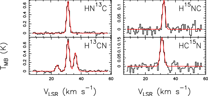
Figure 1: Spectra of the source 18151-1208M1 in all the transitions detected: HN¹³C(1–0) (top-left), H¹⁵NC(1–0) (top-right), H¹³CN(1–0) (bottom-left) and HC¹⁵N(1–0) (bottom-right). For each spectrum the x-axis represents the systemic velocity listed in Tables LABEL:fit1 and LABEL:fit2. The y-axis shows the intensity in main beam temperature units. The red curves are the best fits obtained with MADCUBA (from the method described in Sect. 3).

2 Source selection and observations

2.1 Source sample

The source list of the 66 sources is reported in Table LABEL:tab-coo, where the source coordinates and the distances from the Sun are shown. A part of the source sample was compiled from a list of high-mass young stellar objects from northern millimeter continuum surveys (Sridharan et al. 2002, Beuther et al. 2002). We selected 35 sources with (i) distances < 5 kpc, to sample comparable spatial scales, (ii) strong (peak intensity > 0.5 Jy/beam) and compact 1.2 mm continuum emission, suggestive of high-mass young objects embedded in dust, and (iii) observable with the IRAM-30m telescope. Note that we do not consider any criteria related to the line intensity or molecular richness of the source, nor do we consider the centimeter continuum emission and luminosity, in order to avoid possible biases. The sources cover a broad range of luminosities and evolutionary stages (traced with different star formation signposts, e.g. presence of masers, infrared sources, HII regions) which will permit to study the dependence of chemical properties with luminosity and evolutionary stage. This sample is not classified in evolutionary stages (like that of Colzi et al. 2018), yet. This classifation will be done in a forthcoming paper (Mininni et al., in prep). The whole sample and their properties will be presented in the forthcoming paper, while in this paper we focus on the lines of the isotopologues of HCN and HNC. The other 31 sources, indicated with ^∗∗ in Table LABEL:tab-coo, were selected from the literature (Fontani et al. 2011, Wouterloot et al. 1993, Beltrán et al. 2016, Cesaroni et al. 2017, Tan et al. 2014).

The distances are kinematic distances based on the rotation curve of the Galaxy, and are taken from Sridharan et al. (2002), Beuther et al. (2002) and from the other works cited above. For the sources with the ambiguity of distance we have chosen the near one.

The sample of 66 sources was implemented with that observed by Colzi et al. (2018) of 27 sources, to obtain a statistically significant sample. The sample of 27 sources was divided in the three evolutionary stages: 11 high-mass starless cores (HMSCs), 9 high-mass protostellar objects (HMPOs), and 7 ultra-compact Hii regions (UC HIIs), respectively (see Fontani et al. 2011). Because 6 sources of the two samples were in common: 00117+6412M1, 18089-1732M1, 18517+0437M1, G75, 20081+3122M2 and NGC7538IRS9, we have decided to keep the results found in Colzi et al. (2018) as the S/N of their observations is better than that of the observations presented here by a factor of $\sim$2 (compare spectra in Appendix B of this paper and Appendix B of Colzi et al. 2018). Despite the ratios found in Colzi et al. (2018) were derived using the kinetic temperatures calculated from ammonia (given in Fontani et al. 2011), that are different from the excitation temperature (T_ex) adopted in this work, the ¹⁴N/¹⁵N ratios are almost independent (differences of 1–10%) from the chosen temperature (see Sect. 3), and then their results could be used to increment our sample.

We finally have a sample of 87 sources: the 27 of Colzi et al. (2018) and the 60 of this work not in common with the previous one.

2.2 Observations

The 66 sources analyzed in this work were observed with the IRAM 30m telescope on August 2014. We have used the FTS spectrometer (Fast Fourier Transform Spectrometer; Klein et al. 2012) to cover the frequency range 85.7–93.5 GHz with a frequency resolution of 200 kHz, corresponding to 0.6 km s^-1 at the observed frequencies. The half power beam width (HPBW) is about 29 arcsec. The observations were made in position-switching mode. Pointing was checked every 1.5 hours, and focus was corrected at the beginning of the observations and every 4-6 hours. The integration time ranged from 10 to 30 minutes, except for some sources, as 04579+4703, for which it was less (about 5 minutes). The r.m.s. noise levels of the spectra are presented in Appendix LABEL:fit1, LABEL:fit2, LABEL:fit3 and LABEL:fit4. The system temperature was in the range 100–150 K during the observations. The observed spectra were first calibrated and reduced using the CLASS/GILDAS package (Pety et al. 2005), the data were corrected for platforming and spike channels were removed. The beam efficiency ($B_{\rm eff}$) for the IRAM 30m telescope at these frequencies is 0.86, while the forward efficiency ($F_{\rm eff}$) is 0.95. The antenna temperatures were converted to main beam temperatures by using the expression: $T_{\rm A}^{*}$ = $T_{\rm MB}\eta_{\rm MB}$, where $\eta_{\rm MB}$ = $B_{\rm eff}$/$F_{\rm eff}$. The spectra obtained were exported from the software package CLASS of GILDAS to MADCUBA (see e.g. Rivilla et al. 2016, Rivilla et al. 2017). With MADCUBA we have selected the part of the spectra around the four targeted lines, and we have fitted the baselines with a maximum order of 1. MADCUBA was then used to identify the lines and analyze them. For the analysis we have used the spectroscopic parameters from the Jet Propulsion Laboratory (JPL) molecular catalog. Rest frequencies are taken from the laboratory works and quantum-chemical calculations cited in Table LABEL:observation.

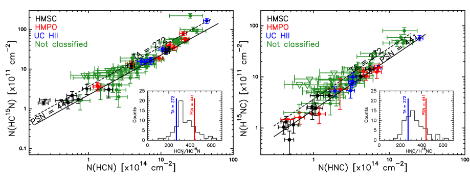
Figure 2: Column densities of HCN against those of HC¹⁵N (left panel) and of HNC against those of H¹⁵NC (right panel). HCN and HNC column densities are derived from those of H¹³CN and HN¹³C, respectively (see Sect. 3). In all panels the filled circles represent the detected sources and the open triangles are the upper limits for the corresponding column densities. In green the 60 sources of this work, in black, red and blue the 27 sources of Colzi et al. (2018) divided in the three evolutionary stages: high-mass starless cores (HMSCs), high-mass protostellar objects (HMPOs), and ultra-compact Hii regions (UC HIIs), respectively. The dashed line indicates the mean atomic composition as measured in the terrestrial atmosphere (TA) and the solid line that measured in the Proto-Solar Nebula (PSN). In the lower right corner of each panel we show the distribution of ¹⁴N/¹⁵N values for HCN (left) and HNC (right). Here the blue vertical line represents the TA value and the red vertical line the PSN value.

3 Analysis and results

3.1 Line detection and fitting procedure

We have considered detections of HN¹³C(1–0), H¹⁵NC(1–0), H¹³CN(1–0), and HC¹⁵N(1–0) if the spectral lines show a peak main beam temperature (T${}_{\rm MB}^{\rm peak}$)$\geq$3$\sigma$, where $\sigma$ is the r.m.s noise of the spectrum; for the detections close to the 3$\sigma$ limit, we have distinguished between tentative detections ($2.5\sigma\leq T_{\rm MB}^{\rm peak}<3\sigma$) and non detections ($T_{\rm MB}^{\rm peak}<2.5\sigma$). For the non detections we have computed the upper limits for the column densities as explained in Colzi et al. (2018), with average value of the full width at half maximum ($\Delta v_{\rm 1/2}$) of the lines: $\Delta v_{{\rm HN}^{13}{\rm C}}=2.6\pm 0.1$ km s^-1, $\Delta v_{{\rm H}^{13}{\rm CN}}=3.3\pm 0.2$ km s^-1, $\Delta v_{{\rm H}^{15}{\rm NC}}=2.3\pm 0.1$ km s^-1 and $\Delta v_{{\rm HC}^{15}{\rm N}}=3.1\pm 0.2$ km s^-1. The percentage of detected lines (together with tentative tetections) is the following: the HN¹³C line is clearly detected in 58 cores (88%), the H¹³CN line is detected in 58 cores (88%) which, however, are not exactly the same (see Tables LABEL:fit1 and LABEL:fit2), the H¹⁵NC line is detected in 45 cores (68%) and the HC¹⁵N line is detected in 49 cores (74%).

Both HN¹³C(1–0) and H¹³CN(1–0) have hyperfine structure, but we can resolve it only for H¹³CN(1–0) because the line widths found ($\sim$3 km s^-1) are smaller than the separations in velocity of the hyperfine components (e.g. Fig. 1). Conversely, H¹⁵NC(1–0) and HC¹⁵N(1–0) do not have hyperfine structure. All the lines were fitted with single Gaussians, except in the case of H¹³CN(1–0) for which we take into account the hyperfine structure, using same T_ex and $\Delta v_{1/2}$ for each transition. Fitting the HN¹³C(1–0) with a single Gaussian can overestimate the line width. To estimates how much the line widths are overestimated by this simplified approach, when possible, we fitted a line both with one gaussian, and considering the hyperfine structure. We found that with a single Gaussian, the line width is about 10% larger than with the hyperfine structure method.

One of the sources, G31.41+0.31, requires some comments: it is a prototypical hot molecular core (HMC) which harbours deeply embedded young stellar objects (YSOs), and the HMC is separated by $\sim$5” from an ultracompact Hii region (UC HII). Observations with the IRAM Plateau de Bure demonstrated the existence of a velocity gradient across the core (Beltrán et al. 2004 and 2005). Subsequently, observations with the Submillimeter Array confirmed the velocity gradient (Cesaroni et al. 2011), supporting the claim of the presence of a rotating toroid. Moreover, observations of ¹²CO and ¹³CO revealed self-absorption caused by infalling gas close to the HMC (Cesaroni et al. 2011). Therefore, G31.41+0.31 is a very complicated source and, as can be noted from the spectra in Appendix B, there is an evidence of possible self-absorption at the center of the lines (for H¹³CN and HN¹³C in particular) and a distorted line profile due to the possible presence of the rotating toroid at larger scales, together with the possibility of outflows from the center of the HMC (Cesaroni et al. 2017, Beltrán et al., 2018). For these reasons we were not able to fit the lines neither with a single Gaussian nor with the three hyperfine components, because of the complex line shape. All of this makes it very difficult to fit the lines with the approximation used for the other sources; therefore, we decided to exclude this source from the analysis.

For G14.99-0.67, instead, we have identified two velocity components, and fit them simultaneously (G14.99-0.67 and G14.99-2).

All the spectra are shown in Appendix B.

3.2 Column density calculation

To compute the colum densities we have used MADCUBA assuming local thermal equilibrium (LTE) conditions. MADCUBA takes five parameters to model the LTE line profile into account: total column density of the molecule (N), T_ex, $\Delta v_{\rm 1/2}$, peak velocity ($v$), and source angular dimension ($\theta$). The total column densities of all species have been evaluated assuming that the emission fills the telescope beam (i.e. no beam dilution has been applied), since we do not have any measurement of the emitting region in our sources. Therefore, the derived column densities are beam-averaged values. Observations towards low-mass protostars at high-angular resolution with the NOEMA interferometer indicate that the H¹³CN and HC¹⁵N(1–0) line emission is indeed very similar (Zapata et al. 2013, Wampfler et al., personal comunication). Therefore, the assumed filling factor should not influence the ¹⁴N/¹⁵N ratio. We have fitted all the lines fixing also the T_ex. We have used the excitation temperature derived from the K-ladder of the $J$=5-4 transition of the CH₃CN molecule, which is a good thermometer of massive dense cores (e.g. Araya et al. 2005, Purcell et al. 2006). The detailed analysis of this species will be presented in a forthcoming paper (Mininni et al., in prep.). The critical densities of the analysed transitions are relatively high ($\sim$3$\times$10⁵ cm^-3), thus the observed transitions could be in non-LTE conditions. As shown by Daniel et al. (2016), if the excitation temperatures are lower than the kinetic temperatures, the excitation temperature of the less abundant isotopologue (with ¹⁵N) could be different from that of the more abundant one and the isotopic ratio could also be affected. Therefore, we have checked with RADEX how T_ex would change in non-LTE conditions and we have found that the T_ex are lower comparing with those obtained with CH₃CN. However, the T_ex of both isotopologues are similar (within $\sim$16%), being that of the more abundant isotopologue always higher. Therefore, the hypothesis that the rotational levels of the two molecules are populated with the same T_ex is valid, and the column densities are computed with the same formula used in LTE approximation (Caselli & Ceccarelli 2012). Furthermore, we have tested how the ratios can change if we use a non-LTE analysis (RADEX), and we have found that the ratios would be, on average, lower than a factor from 1.1 up to 1.6. However we stress that a precise non-LTE analysis can not be made because we don’t know H₂ column densities and kinetic temperatures of all the sources.

After that, leaving free the other three parameters (N, v and $\Delta v_{\rm 1/2}$), we have used the AUTOFIT tool, which compares automatically the synthetic LTE spectra with the observed spectra, and provides the best non-linear least-squared fit using the Levenberg-Marquardt algorithm. Column densities, line widths, peak velocities and opacity ($\tau$) derived from the fit are given in Tables LABEL:fit1 and LABEL:fit2. It can be seen that all the transitions are optically thin as expected. It should also be noted that the opacities are lower limits of the real opacity of the lines, since we assume that the emission of the lines comes from the entire beam. Despite this, we do not expect much higher opacities, and the transitions can be considered still optically thin. To test this, we have assumed a source size of 10” and found that the $\tau$ values increase at most by a factor 10, so that the values would be $\sim 0.01$–$0.1$. The assumption of optically thin transitions is hence still valid.

In Table LABEL:colden column densities of the main isotopologues and of the corresponding ¹⁵N-bearing species are shown.

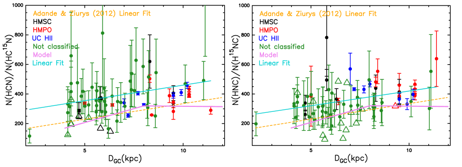
Figure 3: ¹⁴N/¹⁵N ratios for HCN (left panel) and HNC (right panel) as a function of Galactocentric distances of the sources listed in Table LABEL:tab-coo. Symbols are the same of Fig. 2 but the open triangles are lower limits for the corresponding ¹⁴N/¹⁵N ratio. The cyan solid line is the linear regression fit computed for the two data sets and the pink solid line is the model of Romano et al. (2017). The dashed orange line is the regression linear fit obtained by Adande & Ziurys (2012). Note that we used the scale from 50 to 1000 of y-axes for visualization purposes, and that one source for HCN, with value 1305$\pm$650, falls outside.

3.3 ¹⁴N/¹⁵N ratios

The reason why we have observed H¹³CN and HN¹³C is that HNC and HCN are usually optically thick in their lower energy rotational transitions (e.g. Padovani et al. 2011). Hence, we decided to use the ¹³C-bearing species that have been found to be optically thin in high-mass star-forming cores with similar densities (Colzi et al. 2018), and then, the ¹⁴N/¹⁵N ratio was computed from the column density ratio of the two isotopologues and corrected by the ¹²C/¹³C Galactic trend given in Milam et al. (2005):

$${}^{12}\textrm{C}/^{13}\textrm{C}=(6.01\pm 1.19)\textrm{ kpc}^{-1}\times\textrm{D}_{\rm GC}+(12.28\pm 9.33).$$ (1)

This trend is measured with observations of CN, CO and H₂CO in a sample of 18 molecular clouds that lie in the range of Galactocentric distances 0.09–16.41 kpc. Note that ¹³C-fractionation may affect the abundances of ¹³C-bearing species. In fact nitriles and isonitriles are predicted to be significantly depleted in ¹³C (Roueff et al. 2015). However, this depletion is at most of a factor 2 and is derived from a chemical model with a fixed kinetic temperature of 10 K, which probably is not the average kinetic temperature of our sources (see Table LABEL:tab-coo). The predictions of this model may therefore not be appropriate for our objects and observational tests to verify whether this theoretical effect is real have yet to be performed.

We have computed the ¹⁴N/¹⁵N ratios for HNC and HCN, along with uncertainties derived propagating the error on total column densities (Table LABEL:colden). The uncertainties do not include the calibration errors, which cancels out in the ratio because the two lines were obtained in the same spectral setup. In Table LABEL:colden the ¹⁴N/¹⁵N ratios are given.

As discussed in Sect. 2, we have implemented these observations with those made by Colzi et al. (2018). The observations of this sample were made with the same receiver and spectrometer of this work, giving us the possibility to combine the two samples with consistency. For further information about the observations and the results concerning the sample of 27 sources, see Colzi et al. (2018). The isotopic ratios ¹⁴N/¹⁵N, of the whole sample are in the range $\sim$115–1305 from HCN, and in the range $\sim$185–780 from HNC, as can be noted in Table LABEL:colden. All of the ratios found in this work are on average consistent with those computed by Colzi et al. (2018) (Fig. 2). The most direct result of this work, based on an unprecedented statistics, is a firm confirmation of the finding suggested by Colzi et al. (2018): the lowest values found in pristine Solar System material (e.g. $\sim$150 in nitrogen hydrides of some comets, Manfroid et al. 2009) are not typical at the core scales.

In Fig. 2, where the column densities of the two samples are shown, at the bottom right of each panel we have made a histogram, with bin width of 40, that shows the distribution on the ratios. We can note that for both molecules the distribution is asymmetric and centered in the bin 310$\leq^{14}$N/¹⁵N$\leq$350, namely below the PSN value ($\sim$441) and just above the TA value ($\sim$272).

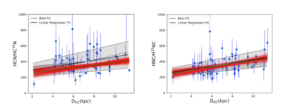
Figure 4: ¹⁴N/¹⁵N ratios for HCN (left panel) and HNC (right panel) as a function of Galactocentric distances of the sources. In all panels only the detection (not the upper limits), are represented with blue filled circles. The red solid lines are all the linear fit found with the Bayesian method, described in text, and the green solid line is the best fit performed with linmix. For comparison we have added with black solid lines the linear regression fits (in grey are represented the errors on this fit), computed as explained in Sect. 3. Note that we used the scale from 50 to 1000 of y-axes for visualization purposes, and that one source for HCN, with value 1305$\pm$650, falls outside.

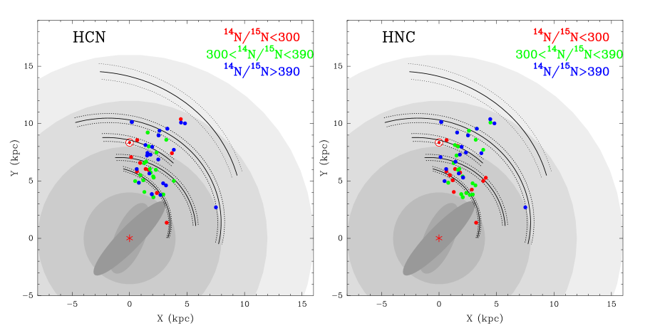
Figure 5: Plan view of the Milky Way. The Galactic center (red asterisk) is at (0,0) and the Sun (red Sun symbol) is at (0,8.34). The background grey discs correspond to the Galactic bar region ($\sim$4 kpc), the solar circle ($\sim$8 kpc), co-rotation of spiral pattern ($\sim$12 kpc) and the edge of major star-formation regions ($\sim$16 kpc). The solid black lines are the center of spiral arms traced by masers, and the dotted lines the 1$\sigma$ widths. For more details see Reid et al. (2014). The filled circles represent sources of our sample implemented with those of Colzi et al. (2018), and the three colors are the ¹⁴N/¹⁵N ratios measured for HCN (left panel) and HNC (right panel): in red ¹⁴N/¹⁵N$\leq$300, in green 300$\leq^{14}$N/¹⁵N$\leq$390 and in blue ¹⁴N/¹⁵N$\geq$390.

3.4 Galactocentric behavior: linear analysis

The merged sample of 87 objects, given by the sources studied in this work and those analysed by Colzi et al. (2018), are located at different distances from the Galactic Centre (D_GC). This gives us the opportunity to study the Galactocentric trend of the ¹⁴N/¹⁵N ratio.

Besides our study, one of the most recent works on the ¹⁴N/¹⁵N Galactocentric gradient is that of Adande & Ziurys (2012). These authors evaluated the ratio from rotational lines of CN, HCN and HNC towards a sample of mixed low- and high-mass star-forming regions observed with different telescopes. In total, their statistics is poorer, as the sample only contains 22 objects. They found an increasing trend of the ¹⁴N/¹⁵N with D_GC and with an unweighted linear regression fit to the data set they obtained:

$${}^{14}\textrm{N}/^{15}\textrm{N}=(21.1\pm 5.2)\textrm{ kpc}^{-1}\times\textrm{D}_{\rm GC}+(123.8\pm 37.1).$$ (2)

Our total sample increases the statistics by a factor 4, and we can properly constrain for the first time the ¹⁴N/¹⁵N Galactocentric trend with this robust statistics. We have chosen to separate the results of the two molecules because the distributions presented in Fig. 2 suggest a possible difference between the two isotopologues. We have first computed an unweighted linear regression fit to the data (excluding the lower limits), in order to compare it to the results of Adande & Ziurys (2012), and found:

$$\textrm{HCN}/\textrm{HC}^{15}\textrm{N}=(21\pm 9)\textrm{ kpc}^{-1}\times\textrm{D}_{\rm GC}+(250\pm 67),$$ (3)

$$\textrm{HNC}/\textrm{H}^{15}\textrm{NC}=(20\pm 6)\textrm{ kpc}^{-1}\times\textrm{D}_{\rm GC}+(221\pm 42).$$ (4)

These trend are shown in Fig. 3. Both slopes are consistent with that found by Adande & Ziurys (2012), and are also consistent with each other. However, we found a general trend that shows an offset of about 100 toward larger values for the ¹⁴N/¹⁵N, as can be noted also in both panels of Fig. 3. We have also tried to fit the data with a single power-law relation using the maximum-likelihood Bayesian tool linmix by Kelly et al. (2007), which derives the linear dependence considering measurement uncertainties (Fig. 4) and excluding the lower limits. The best fits we found are:

$$\textrm{HCN}/\textrm{HC}^{15}\textrm{N}=(17\pm 6)\textrm{ kpc}^{-1}\times\textrm{D}_{\rm GC}+(223\pm 12),$$ (5)

$$\textrm{HNC}/\textrm{H}^{15}\textrm{NC}=(22\pm 6)\textrm{ kpc}^{-1}\times\textrm{D}_{\rm GC}+(198\pm 12).$$ (6)

The linear regression fit is consistent with the best Bayesian fit within the uncertainties, as can be seen in Fig. 4, mostly for HNC. Note that in the case of the Bayesian analysis the errors are lower than in the linear regression fit because in the standard analysis the errors on the parameters are computed separately, as they are considered independent. On the contrary in the Bayesian analysis an optimised procedure, that takes into account the dependence between the two parameters, is performed and converges to the best parameters with lower errors than in the other analysis.

3.4.1 Dependence with spatial distribution in the Galaxy

In order to investigate a dependence with the Galactic longitude ($l$, listed in Table LABEL:tab-coo), we have plotted our results in the Galactic plan view of the Milky Way made by Reid et al. (2014). The solid curved lines trace the center of spiral arms as measured with masers associated with young, high-mass stars. We have plotted in the Galactic plane the position of our sources and we have divided the ratio in three intervals: ¹⁴N/¹⁵N$\leq$300, 300$\leq$ ¹⁴N/¹⁵N$\leq$390 and ¹⁴N/¹⁵N$\geq$390 (Fig. 5). We have decided to use these ranges because each of them contains a similar number of objects. For both molecules no clear trend along spiral arms was found. We have also checked if there was any residual trend after substracting to all the ¹⁴N/¹⁵N ratios the values obtained at the correponding D_GC of the source with the Bayesian fit, but we have not found trends either. Thus, we conclude that the Galactocentric gradient, probably, is related only to the source distances and not to other local processes.

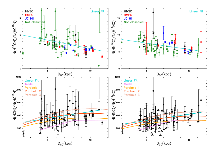
Figure 6: Upper panels: ¹³C¹⁴N/¹²C¹⁵N ratios for HCN (left panel) and HNC (right panel) as a function of Galactocentric distances of the sources. Symbols are the same of Fig. 3 and the cyan solid line is the linear regression fit computed from the two data sets. Note that the negative slope is the consequence of the two combined ratios, ¹³C/¹²C and ¹⁴N/¹⁵N. Bottom panels: same of Fig. 3 with all the sources in black, while the three parabolas are described in Sect. 3.5. The yellow one is found using the minimum value in slope of Eq. (1) (Parabola 1), the red one is found using the central value of the slope (Parabola 2) and the pink one is found using the maximum value of the slope (Parabola 3). Note that we used the scale from 50 to 1000 of y-axes for visualization purposes, and that one source for HCN, with value 1305$\pm$650, falls outside.

3.5 Galactocentric behavior: parabolic analysis

The linear analysis relies on the ¹²C/¹³C relation by Milam et al. (2005) (Eq. (1)), that we have assumed to compute ¹⁴N/¹⁵N ratios. Note that what can be measured directly from our observations are the H¹³CN/HC¹⁵N and HN¹³C/H¹⁵NC ratios. In the upper panels of Fig. 6 these ratios have been plotted as a function of the Galactocentric distances, and, since the points suggest a negative linear trend, we have computed unweighted linear regression fits to these data, obtaining:

$$\textrm{H}^{13}\textrm{CN}/\textrm{HC}^{15}\textrm{N}=(-0.5\pm 0.2)\textrm{ kpc}^{-1}\times\textrm{D}_{\rm GC}+(11.0\pm 1.2),$$ (7)

$$\textrm{HN}^{13}\textrm{C}/\textrm{H}^{15}\textrm{NC}=(-0.4\pm 0.1)\textrm{ kpc}^{-1}\times\textrm{D}_{\rm GC}+(9.4\pm 0.8).$$ (8)

We have tested the linearity of this relation also using a non-parametric statistics that allows to explore the data sets without assuming an underlying model that describes the data, finding a linear trend of the ratios with the Galactocentric distances. The ¹⁴N/¹⁵N ratios, that have been derived in this work, are the product between ¹⁴N¹³C/¹⁵N¹²C and ¹²C/¹³C. Considering that ¹⁴N¹³C/¹⁵N¹²C ratios are well fitted by a linear trend, and the assumption that ¹²C/¹³C is also linear with D_GC (Milam et al. 2005), then the derived ¹⁴N/¹⁵N must have a parabolic one. The parabolas have equations, for HNC and HCN, respectively:

$$\begin{split}&\textrm{HCN}/\textrm{HC}^{15}\textrm{N}=[(-0.5\pm 0.2)\textrm{ kpc}^{-1}\times\textrm{D}_{\rm GC}+(11.0\pm 1.2)]\times\\ &\times[^{12}\textrm{C}/^{13}\textrm{C}],\end{split}$$ (9)

$$\begin{split}&\textrm{HNC}/\textrm{H}^{15}\textrm{NC}=[(-0.4\pm 0.1)\textrm{ kpc}^{-1}\times\textrm{D}_{\rm GC}+(9.4\pm 0.8)]\times\\ &\times[^{12}\textrm{C}/^{13}\textrm{C}].\end{split}$$ (10)

In the bottom panels of Fig. 6 the three parabolas obtained choosing the slope of ¹²C/¹³C as the minimum, the centered and the maximum in the error, are plotted. Interestingly, with this analysis we are able to reproduce the flattening trend above $\sim$8 kpc predicted by the GCE model of Romano et al. (2017). This is the distance where the parabolic trend start to disagree with the linear trend of the linear analysis. This result remains the same whatever the assumption of the ¹²C/¹³C.

4 Discussion and Conclusions

We have observed the rotational transitions J=1-0 of HN¹³C, H¹⁵NC, H¹³CN and HC¹⁵N towards 66 massive star-forming cores to derive the ¹⁴N/¹⁵N ratios. We have complemented this sample with that observed by Colzi et al. (2018), obtaining a total sample of 87 sources. The isotopic ratios measured range from 115 up to 1305 for HCN and from 185 up to 780 for HNC, which are higher than the low values in the pristine Solar System material.

With the strong statistics of 87 sources a new Galactocentric trend has been derived. From the linear fits given in Eq. (5) and (6), we derive that the ¹⁴N/¹⁵N ratios in the local interstellar medium (ISM), i.e. the values calculated at the Galactocentric distance of the Sun (8.4 kpc, Reid et al. 2009), are 383$\pm$51 for HCN and 366$\pm$51 for HNC. These values are both higher than 301$\pm$44 which was obtained from the gradient of Adande & Ziurys (2012). Despite the large uncertainties, our new local interstellar values are more similar to the PSN value of $\sim$441, measured from the Solar wind adopting a totally different approach (Marty et al. 2010).

Let us now discuss briefly our findings in the general context of the origin of ¹⁴N and ¹⁵N in the Galaxy. As discussed in Sect.1, primary contributors to ¹⁴N are massive stars in He-shell burning, while the main contributor of ¹⁵N, which is a secondary element, is the hot CNO cycle in novae outbursts. In our Galaxy the abundance of heavy elements is found to decrease with the distance, as observed by Maciel & Costa (2009). Therefore the ¹⁴N/¹⁵N ratio should increase with Galactocentric distance as the main contributors of ¹⁵N are novae and some supernovae events (for example, Romano et al. 2017). The positive trend found with the Galactocentric distance suggests that there is not a primary component production of ¹⁵N, that is instead important for ¹⁴N in the environment with an high rate of star formation, like at D_GC<8 kpc. The slope of the GCE model of Romano et al. (2017), which takes novae as the main contributors of ¹⁵N into account, is in agreement with our observational results (Fig. 3), up to 8 kpc. Then, up to 12 kpc the curve in the model flattens. With our linear fit we can not say what is happening after 8 kpc as the linear trend can be biased by points at smaller distances.

A second analysis points out a parabolic trend of ¹⁴N/¹⁵N ratios with the Galactocentric distance. This is based taking into account the linear assumption made for the ¹²C/¹³C ratios (Milam et al. 2005). With this analysis we were able to reproduce the flattening trend above 8 kpc, as predicted by the GCE model of Romano et al. (2017). The flattening of the ¹⁴N/¹⁵N gradient for D${}_{\rm GC}>$ 8 kpc in the model of Romano et al. (2017) is due to the absence of substantial ¹⁴N-enrichment from low-metallicity massive stars (Nomoto et al. 2013).

Note that the model is a lower limit of the ¹⁴N/¹⁵N ratios found (Fig. 3 and bottom panels of Fig. 6). An interpretation of this result could be that the first N-fractionation is regulated by the nucleosynthesis processes, and afterwards there could be local (at core level) enrichments of ¹⁴N/¹⁵N.

Of course, to confirm our results, more observations of sources in the outer Galaxy are needed. New observations could place important constraints on the amount of ¹⁴N produced by massive stars in low-metallicity environments. The trend we have found in our Milky Way can be relevant also as "template" for extra-galactic sources, in which the ¹⁴N/¹⁵N has been measured in a few objects. For example, toward the massive star forming region N113 in the Large Magellanic Cloud a ¹⁴N/¹⁵N ratio of 111$\pm$17 was found (Chin et al. 1999). Toward the nuclear region of nearby Seyfert 2 galaxy NGC 1068 a ¹⁴N/¹⁵N ratio greater than 419 was found (Wang et al. 2014). Toward the z=0.89 spiral galaxy, located on the line of sight to the quasar PKS1830-211, a ratio of 152$\pm$27 was measured (Muller et al. 2011). Moreover, through millimeter molecular absorption lines arising in the z=0.68 absorber toward B0218+357, a ratio of $\sim$120 was measured (Wallström et al. 2016). These measurements indicate that even in external galaxies the ¹⁴N/¹⁵N is far from being homogeneous. We stress, however, that the comparison between local clouds in the Milky Way and external galaxies should be taken with caution. In this kind of sources the relative contribution of the processes responsible for changes in the ¹⁴N/¹⁵N (nucleosynthesis and/or chemical fractionation), has not been explored. Moreover, it is difficult to determine local trends because the single clouds cannot be resolved easily.

Table 2: List of the observed sources. Cols. 2, 3, 4 and 5 give the coordinates (equatorial and Galactic) of the sources and Col. 6 give the source distance to the Sun of the associated star-forming region. In Col. 7 the Galactocentric distances of the sources obtained from the distance to the Sun and the corresponding Galactic longitude (Col. 4) are listed. In Col. 8 we give the T_ex used to fit the lines for all the sources, computed as explained in Sect. 3. The T_ex have been derived fitting the K-ladder of CH₃CN(5–4) (Mininni et al., in prep.).

Source	$\alpha({\rm J2000})$	$\delta({\rm J2000})$	$l$	$b$	$d$	DGC	Tex
	(h m s)	($\degr$ $\arcmin$ $\arcsec$)	($\degr$)	($\degr$)	(kpc)	(kpc)	(K)
I00117-MM1∗∗	00:14:26.1	+64:28:44.0	118.96	+1.89	1.8	9.4	35∗∗∗
I04579-VLA1∗∗	05:01:39.9	+47:07:21.0	160.14	+3.16	2.5	10.7	35∗∗∗
18089-1732M1	18:11:51.5	-17:31:29.0	12.89	+0.49	3.6*	4.9	87
18089-1732M4	18:11:54.0	-17:29:59.0	12.92	+0.49	3.6*	4.9	36
18151-1208M1	18:17:58.0	-12:07:27.0	18.34	+1.77	3.0	5.6	37
18151-1208M2	18:17:50.4	-12:07:55.0	18.32	+1.79	3.0	5.6	42
18182-1433M1	18:21:09.2	-14:31:49.0	16.59	-0.05	4.5*	4.2	52
18264-1152M1	18:29:14.6	-11:50:22.0	19.88	-0.53	3.5*	5.2	50
18272-1217M1	18:30:02.9	-12:15:17.0	19.61	-0.90	2.9	5.7	52
18290-0924M2	18:31:46.3	-09:22:23.0	22.36	+0.06	5.3*	4.0	–
18306-0835M1	18:33:24.0	-08:33:31.0	23.27	+0.08	4.9*	4.3	39
18306-0835M2	18:33:17.2	-08:33:26.0	23.25	+0.10	4.9*	4.3	36
18308-0841M1	18:33:33.1	-08:39:10.0	23.20	-0.00	4.9*	4.3	36
18310-0825M2	18:33:44.0	-08:21:20.0	23.48	+0.10	5.2*	4.1	38
18310-0825M3	18:33:42.2	-08:21:36.0	23.48	+0.10	5.2*	4.1	34
18372-0541M1	18:39:56.0	-05:38:47.0	26.60	-0.02	1.8*	6.8	71
18385-0512M1	18:41:13.3	-05:09:01.0	27.19	-0.08	2.0*	6.6	49
18445-0222M3	18:47:07.7	-02:21:26.0	30.34	-0.12	5.3*	4.6	15
18454-0136M1	18:48:02.5	-01:33:26.0	31.16	+0.05	2.7*	6.2	33
18472-0022M1	18:49:52.4	-00:18:56.0	32.47	+0.20	3.2*	5.9	32
18488+0000M1	18:51:25.6	+00:04:06.0	32.99	+0.03	5.4*	4.8	36
18517+0437M1	18:54:14.3	+04:41:40.0	37.43	+1.5	2.9	6.3	41
18521+0134M1	18:54:40.8	+01:38:05.0	34.76	+0.02	5.0*	5.1	37
19012+0536M1	19:03:45.4	+05:40:43.0	39.39	-0.14	4.6*	5.6	37
19035+0641M1	19:06:01.6	+06:46:43.0	40.62	-0.14	2.2	6.8	49
19095+0930	19:11:54.0	+09:35:52.0	43.80	-0.13	3.3	6.4	57
19282+1814M1	19:30:23.1	+18:20:25.0	53.62	+0.03	1.9*	7.4	44
19410+2336M1	19:43:10.9	+23:44:10.0	59.78	+0.07	2.1*	7.5	32
19411+2306M1	19:43:18.0	+23:13:59.0	59.36	-0.21	2.9*	7.3	27
19413+2332M1	19:43:29.3	+23:40:18.0	59.76	-0.03	1.8*	7.6	36
ON1∗∗	20:10:09.1	+31:31:36.0	69.54	-0.98	2.5	7.8	85
20126+4104M1	20:14:25.9	+41:13:34.0	78.12	+3.63	1.7	8.2	71
20216+4107M1	20:23:23.5	+41:17:38.0	79.13	+2.28	1.7	8.2	54
20319+3958M1	20:33:49.1	+40:08:35.0	79.35	+0.00	1.6	8.2	58
20332+4124M1	20:34:59.7	+41:34:49.0	80.63	+0.68	3.9	8.6	35∗∗∗
20343+4129M1	20:36:07.9	+41:39:57.0	80.83	+0.57	1.4	8.2	52
22187+5559V3∗∗	22:20:33.7	+56:14:29.1	103.06	-0.69	2.9	9.4	–
22187+5559V5∗∗	22:20:35.6	+56:14:46.4	103.06	-0.69	2.9	9.4	–
22198+6336∗∗	22:21:26.8	+63:51:37.2	107.30	+5.64	0.7	8.6	64
22570+5912M2	22:58:59.2	+59:27:36.0	109.08	-0.35	5.1	11.1	35∗∗∗
23033+5951M1	23:05:25.3	+60:08:06.0	110.09	-0.07	3.5	10.1	26
23139+5939M1	23:16:10.5	+59:55:28.0	111.26	-0.77	4.8	11.0	39
G75-core∗∗	20:21:44.0	+37:26:38.0	75.78	+0.34	3.8	8.3	56
G08.14+0.22∗∗	18:03:01.3	-21:48:05.0	8.14	+0.22	3.4	5.0	52
G14.33-0.65∗∗	18:18:54.8	-16:47:53.0	14.33	-0.65	2.6	5.9	49
G14.99-0.67∗∗	18:20:17.6	-16:13:55.0	14.99	-0.67	2.4	6.0	22
G14.99-2∗∗	18:20:17.6	-16:13:55.0	14.99	-0.67	2.4	6.0	35∗∗∗
G15.02-0.62∗∗	18:20:10.3	-16:10:35.0	15.02	-0.62	2.4	6.1	14
G24.78+0.08∗∗	18:36:12.6	-07:12:10.9	24.79	+0.08	7.7	2.1	93
G31.41+0.31∗∗	18:47:34.2	-01:12:45.0	31.41	+0.31	7.9	3.5	–
G34.82+0.35∗∗	18:53:37.4	+01:50:32.0	34.82	+0.35	3.6	5.6	35
G35.03+0.35∗∗	18:54:00.6	+02:01:19.3	35.02	+0.35	3.2	6.0	40
G35.20-0.74∗∗	18:58:13.0	+01:40:36.0	35.20	-0.74	2.2	6.7	50
G36.70+0.09∗∗	18:57:59.3	+03:24:05.0	36.71	+0.10	9.7	5.6	–
G37.55+0.19∗∗	18:59:11.4	+04:12:14.0	37.56	+0.20	5.6	5.1	44
G40.28-0.22∗∗	19:05:42.1	+06:26:08.0	40.28	-0.22	4.9	5.4	43
G42.03+0.19∗∗	19:07:29.0	+08:10:39.0	42.03	+0.19	11.1	7.2	–
G42.30-0.30∗∗	19:09:44.2	+08:11:33.0	42.30	-0.30	10.5	7.0	35∗∗∗
G42.70-0.15∗∗	19:09:55.8	+08:36:56.0	42.70	-0.15	15.9	11.2	–
G48.99-0.30∗∗	19:22:26.3	+14:06:37.0	48.99	-0.30	5.1	5.8	37
G49.41+0.33∗∗	19:20:58.9	+14:46:46.0	49.41	+0.33	12.2	9.2	–
G50.78+0.15∗∗	19:24:17.2	+15:53:54.0	50.78	+0.15	7.0	6.5	–
G52.92+0.41∗∗	19:27:35.2	+17:54:26.0	52.92	+0.41	5.1	6.5	–
G53.04+0.11∗∗	19:28:55.7	+17:52:01.0	53.04	+0.11	9.4	8.0	32
G53.14+0.07∗∗	19:29:17.5	+17:56:24.0	53.14	+0.07	1.9	7.4	42
NGC7538-IRS1∗∗	23:13:43.3	+61:28:10.6	111.54	+0.78	2.8	7.0	43
NGC7538-IRS9∗∗	23:14:01.8	+61:27:20.0	111.57	+0.75	2.8	9.7	39

* sources with distance ambiguity, due to their posiition within the Solar circle, for which we have chosen the near distance. For details see Sridharan et al. (2002).
^∗∗ sources selected from the literature (Fontani et al. 2011, Wouterloot et al. 1993, Beltrán et al. 2016, Cesaroni et al. 2017, Tan et al. 2014).
^∗∗∗ sources for which it was not possible to obtain T_ex from CH₃CN and then we have used a T_ex of 35 K, which is the mean value of the excitation temperatures of the sources.

Table 3: Total column densities of observed transitions, and ¹⁴N/¹⁵N ratios. In Cols. 2, 3, 4 and 5 are listed the total column densities (beam-averaged), computed as explained in Sect. 3, of HN¹³C, H¹⁵NC, H¹³CN and HC¹⁵N. In Col. 6 and 7 the ¹⁴N/¹⁵N ratios for HNC and HCN are listed. In Col. 8 the¹²C/¹³C ratio, used to compute the ratio, are listed.

Source	N(HN13C)	N(H15NC)	N(H13CN)	N(HC15N)	$\frac{HNC}{H^{15}NC}$	$\frac{HCN}{HC^{15}N}$	12C/13C
	($\times$1012cm-2)	($\times$1011cm-2)	($\times$1012cm-2)	($\times$1011cm-2)
I00117-MM1	1.5$\pm$ 0.3	$\leq$5.9	2.7 $\pm$ 0.4	5 $\pm$ 2 t	$\geq$174	370 $\pm$ 139	68
I04579-VLA1	$\leq$1.1	$\leq$ 10.1	4.2$\pm$0.8	$\leq$11	–	$\geq$293	77
18089-1732M1	35 $\pm$ 4	47 $\pm$ 8	78 $\pm$ 9	140 $\pm$ 20	311 $\pm$ 97	233 $\pm$ 68	42
18089-1732M4	3.5 $\pm$ 0.5	6 $\pm$ 2	7.0 $\pm$ 1.0	7 $\pm$ 2	244 $\pm$ 92	418 $\pm$ 151	42
18151-1208M1	8 $\pm$ 1	15 $\pm$ 3	14 $\pm$ 2	23 $\pm$ 4	244 $\pm$ 74	279 $\pm$ 88	46
18151-1208M2	8 $\pm$ 1	13 $\pm$ 3	14 $\pm$ 2	18 $\pm$ 4	282 $\pm$ 101	356 $\pm$ 118	46
18182-1433M1	16 $\pm$ 2	25 $\pm$ 4	40 $\pm$ 4	48 $\pm$ 6	241 $\pm$ 76	314 $\pm$ 99	38
18264-1152M1	15 $\pm$ 2	29 $\pm$ 4	36 $\pm$ 4	48 $\pm$ 7	225 $\pm$ 66	326 $\pm$ 96	43
18272-1217M1	1.4$\pm$ 0.3	$\leq$7.1	4.5$\pm$0.7	$\leq$9.3	$\geq$92	$\geq$225	46
18290-0924M2	$\leq$0.6	$\leq$6.2	$\leq$1	$\leq$7.1	–	–	36
18306-0835M1	10 $\pm$ 1	10 $\pm$ 2	21 $\pm$ 3	17 $\pm$ 3	382 $\pm$ 131	471 $\pm$ 152	38
18306-0835M2	4.7$\pm$ 0.6	$\leq$4.4	6.9 $\pm$ 0.9	4 $\pm$ 2	$\geq$408	658 $\pm$ 296	38
18308-0841M1	9 $\pm$ 1	10 $\pm$ 2	12 $\pm$ 2	11 $\pm$ 3	343 $\pm$ 118	416 $\pm$ 166	38
18310-0825M2	9 $\pm$ 1	10 $\pm$ 1	17 $\pm$ 2	19 $\pm$ 4	334 $\pm$ 101	332 $\pm$ 117	37
18310-0825M3	6.0 $\pm$ 0.8	7 $\pm$ 2	5.9 $\pm$ 0.8	8 $\pm$ 3t	318 $\pm$ 120	274 $\pm$ 155	37
18372-0541M1	3.5$\pm$ 0.7	$\leq$1.2	12$\pm$1	$\leq$13	$\geq$155	$\geq$490	53
18385-0512M1	1.7$\pm$ 0.4	$\leq$9.1	8 $\pm$ 1	19 $\pm$ 5	$\geq$97	217 $\pm$ 76	52
18445-0222M3	1.6 $\pm$ 0.2	2.0 $\pm$ 0.9	1.9 $\pm$ 0.3	1.6 $\pm$ 0.6	321 $\pm$ 169	476 $\pm$ 236	40
18454-0136M1	2.9 $\pm$ 0.5	5 $\pm$ 1	2.0 $\pm$ 0.5	6 $\pm$ 2	287 $\pm$ 112	165 $\pm$ 65	49
18472-0022M1	4.5 $\pm$ 0.6	5 $\pm$ 2	5.1 $\pm$ 0.7	3 $\pm$ 1	430 $\pm$ 167	812 $\pm$ 406	48
18488+0000M1	6.5 $\pm$ 0.8	7 $\pm$ 1	14 $\pm$ 2	15 $\pm$ 2	383 $\pm$ 128	385 $\pm$ 120	41
18517+0437M1	7.8 $\pm$ 0.9	13 $\pm$ 2	23 $\pm$ 2	35 $\pm$ 4	301 $\pm$ 85	329 $\pm$ 89	50
18521+0134M1	3.1 $\pm$ 0.5	5 $\pm$ 2	4.8$\pm$0.7	$\leq$6.3	267 $\pm$ 107	$\geq$328	43
19012+0536M1	3.5 $\pm$ 0.5	5 $\pm$ 1t	11 $\pm$ 1	12 $\pm$ 2	322 $\pm$ 126	422 $\pm$ 131	46
19035+0641M1	6.6$\pm$ 0.9	$\leq$7.4	9 $\pm$ 1	14 $\pm$ 4 t	$\geq$476	343 $\pm$ 134	53
19095+0930	9$\pm$ 1	$\leq$9.4	35 $\pm$ 4	46 $\pm$ 8	$\geq$485	385 $\pm$ 117	51
19282+1814M1	4.0 $\pm$ 0.6	7 $\pm$ 2	3.8 $\pm$ 0.6	4 $\pm$ 2	324 $\pm$ 106	538 $\pm$ 226	57
19410+2336M1	7.2 $\pm$ 0.9	14 $\pm$ 2	14 $\pm$ 2	19 $\pm$ 3	295 $\pm$ 78	423 $\pm$ 112	57
19411+2306M1	1.9$\pm$ 0.3	$\leq$5.3	2.6 $\pm$ 0.5	3 $\pm$ 1	$\geq$202	487 $\pm$ 241	56
19413+2332M1	2.6$\pm$ 0.4	$\leq$5.1	6.5 $\pm$ 0.8	6 $\pm$ 2	$\geq$296	628 $\pm$ 220	58
ON1	24 $\pm$ 3	40 $\pm$ 9	35 $\pm$ 4	55 $\pm$ 9	356 $\pm$ 113	378 $\pm$ 103	59
20126+4104M1	26 $\pm$ 3	51 $\pm$ 7	31 $\pm$ 4	59 $\pm$ 9	313 $\pm$ 82	323 $\pm$ 87	61
20216+4107M1	4.8 $\pm$ 0.7	10 $\pm$ 3	4.5 $\pm$ 0.7	9 $\pm$ 3	296 $\pm$ 111	306 $\pm$ 122	62
20319+3958M1	2.8 $\pm$ 0.4	7 $\pm$ 2	3.2$\pm$0.5	$\leq$8.2	246 $\pm$ 81	$\geq$240	62
20332+4124M1	1.6 $\pm$ 0.3	3 $\pm$ 1t	3.4 $\pm$ 0.5	4 $\pm$ 1	342 $\pm$ 157	545 $\pm$ 227	64
20343+4129M1	9 $\pm$ 1	18 $\pm$ 4	10 $\pm$ 1	12 $\pm$ 3	309 $\pm$ 95	515 $\pm$ 179	62
22187+5559V3	$\leq$0.6	$\leq$ 5.6	$\leq$0.6	$\leq$6.3	–	–	69
22187+5559V5	$\leq$0.7	$\leq$ 6.7	$\leq$0.8	$\leq$7.2	–	–	69
22198+6336	5.4 $\pm$ 0.7	12 $\pm$ 3	6.3 $\pm$ 0.9	16 $\pm$ 3	287 $\pm$ 83	251 $\pm$ 79	64
22570+5912M2	2.1 $\pm$ 0.3	3 $\pm$ 1 t	3.3 $\pm$ 0.5	2.0 $\pm$ 0.9t	554 $\pm$ 250	1305 $\pm$ 650	79
23033+5951M1	4.3 $\pm$ 0.6	9 $\pm$ 2	9 $\pm$ 1	14 $\pm$ 3	349 $\pm$ 104	469 $\pm$ 127	73
23139+5939M1	2.3 $\pm$ 0.4	6 $\pm$ 2	10 $\pm$ 1	116 $\pm$ 3	301 $\pm$ 145	491 $\pm$ 130	79
G75-core	9 $\pm$ 1	27 $\pm$ 5	40 $\pm$ 5	72 $\pm$ 10	207 $\pm$ 59	345 $\pm$ 90	62
G08.14+0.22	14 $\pm$ 2	15 $\pm$ 4	27 $\pm$ 3	36 $\pm$ 7	395 $\pm$ 158	318 $\pm$ 102	42
G14.33-0.65	30 $\pm$ 3	59 $\pm$ 8	59 $\pm$ 7	100 $\pm$ 10	242 $\pm$ 68	280 $\pm$ 78	47
G14.99-0.67	8 $\pm$ 2	15 $\pm$ 4	10 $\pm$ 2	11 $\pm$ 4	257 $\pm$ 105	439 $\pm$ 200	48
G14.99-2	3.4 $\pm$ 0.5	9 $\pm$ 2	4.0 $\pm$ 0.8	7 $\pm$ 2	184 $\pm$ 58	278 $\pm$ 94	49
G15.02-0.62	5 $\pm$ 0.9	6 $\pm$ 1	8 $\pm$ 1	12 $\pm$ 2	406 $\pm$ 141	325 $\pm$ 98	49
G24.78+0.08	62 $\pm$ 7	80 $\pm$ 10	100 $\pm$ 10	220 $\pm$ 30	197 $\pm$ 81	116 $\pm$ 47	25
G31.41+0.31	–	–	–	–	–	–	33
G34.82+0.35	6.2 $\pm$ 0.9	9 $\pm$ 3	7 $\pm$ 1	10 $\pm$ 2	316 $\pm$ 130	322 $\pm$ 104	46
G35.03+0.35	8 $\pm$ 1	15 $\pm$ 4	34 $\pm$ 4	47 $\pm$ 7	258 $\pm$ 100	350 $\pm$ 99	48
G35.20-0.74	29 $\pm$ 3	46 $\pm$ 8	60 $\pm$ 7	90 $\pm$ 10	330 $\pm$ 95	349 $\pm$ 94	52
G36.70+0.09	1.8$\pm$ 0.3	$\leq$7	$\leq$0.8	$\leq$7.8	$\geq$118	–	46
G37.55+0.19	7$\pm$ 1	$\leq$8.6	8$\pm$1	$\leq$9.5	$\geq$350	$\geq$362	43
G40.28-0.22	7 $\pm$ 1	10 $\pm$ 3	18 $\pm$ 2	18 $\pm$ 5	312 $\pm$ 124	446 $\pm$ 165	45
G42.03+0.19	$\leq$0.7	$\leq$5.7	$\leq$0.7	$\leq$6.5	–	–	55
G42.30-0.30	2.8$\pm$ 0.4	$\leq$5.6	2.4$\pm$0.4	$\leq$6.8	$\geq$273	$\geq$193	55
G42.70-0.15	$\leq$0.7	$\leq$6	$\leq$0.7	$\leq$7	–	–	80
G48.99-0.30	27 $\pm$ 3	46 $\pm$ 6	36 $\pm$ 4	48 $\pm$ 6	275 $\pm$ 79	352 $\pm$ 101	47
G49.41+0.33	$\leq$1	$\leq$8.4	$\leq$0.9	$\leq$9.4	–	–	68
G50.78+0.15	3.4$\pm$ 0.5	$\leq$8.7	3.6$\pm$0.6	$\leq$9.3	$\geq$201	$\geq$199	51
G52.92+0.41	2.4 $\pm$ 0.3	5 $\pm$ 2	1.7$\pm$0.3	$\leq$7	246 $\pm$ 95	$\geq$124	51
G53.04+0.11	3.3 $\pm$ 0.5	4 $\pm$ 1	7.8 $\pm$ 1	8 $\pm$ 2	496 $\pm$ 196	586 $\pm$ 186	60
G53.14+0.07	6.0 $\pm$ 0.8	9 $\pm$ 2	22 $\pm$ 3	29 $\pm$ 4	377 $\pm$ 115	429 $\pm$ 114	56
NGC7538-IRS1	7 $\pm$ 1	12 $\pm$ 4	32 $\pm$ 4	55 $\pm$ 9	318 $\pm$ 137	317 $\pm$ 88	55
NGC7538-IRS9	5.0 $\pm$ 0.7	11 $\pm$ 2	18 $\pm$ 2	29 $\pm$ 5	322 $\pm$ 93	439 $\pm$ 119	71

^t tentative detection, as explained in Sect. 3.

Appendix A Fit results

In this appendix, the results of the fitting procedure to the HN¹³C(1-0), H¹⁵NC(1-0), H¹³CN(1-0) and HC¹⁵N(1-0) lines of all sources are shown. The method is explained in Sect. 3.1.

Table 4: Values obtained with the fitting procedure described in Sect. 3 to the HN¹³C lines. In the second and in the third columns the centroid velocities and the FWHM are listed. In the fourth column the total column densities derived for the sources are listed, and in the fifth column there are the opacity of the lines. In the sixth column the r.m.s. of observed lines are listed. The cases in which the line is not detected, and therefore only column density upper limits could be obtained as explained in Sect. 3, are indicated with – .

Source	HN13C(1-0)
	$v_{\rm LSR}$	$\Delta v_{\rm 1/2}$	$N_{\rm tot}$	$\tau$	$\sigma$
	(km s-1)	(km s-1)	($\times$1012cm-2)		(mK)
I00117-MM1	-36.03$\pm$4	1.6$\pm$0.1	1.5$\pm$ 0.3	0.0051$\pm$0.0006	16
I04579-VLA1	–	–	$\leq$1.1	–	27
18089-1732M1	33.02$\pm$0.08	3.8$\pm$0.01	35 $\pm$ 4	0.0087$\pm$0.0004	11
18089-1732M4	33.20$\pm$0.06	1.58$\pm$0.08	3.5 $\pm$ 0.5	0.0120$\pm$0.0008	14
18151-1208M1	33.31$\pm$0.04	2.01$\pm$0.05	8 $\pm$ 1	0.0211$\pm$0.0007	15
18151-1208M2	29.78$\pm$0.07	2.51$\pm$0.07	8 $\pm$ 1	0.0126$\pm$0.0005	15
18182-1433M1	59.86$\pm$0.06	3.42$\pm$0.07	16 $\pm$ 2	0.0123$\pm$0.0004	9
18264-1152M1	43.68$\pm$0.05	2.76$\pm$0.05	15 $\pm$ 2	0.0156$\pm$0.0004	10
18272-1217M1	34.0$\pm$0.1	1.6$\pm$0.2	1.4$\pm$ 0.3	0.0023$\pm$0.0002	14
18290-0924M2	–	–	$\leq$0.6	–	15
18306-0835M1	78.15$\pm$0.05	2.53$\pm$0.04	10 $\pm$ 1	0.0188$\pm$0.0004	11
18306-0835M2	76.7$\pm$0.1	2.23$\pm$0.08	4.7$\pm$ 0.6	0.0112$\pm$0.0005	15
18308-0841M1	76.78$\pm$0.04	2.40$\pm$0.05	9 $\pm$ 1	0.0204$\pm$0.0006	16
18310-0825M2	84.92$\pm$0.08	3.15$\pm$0.09	9 $\pm$ 1	0.0146$\pm$0.0006	15
18310-0825M3	85.71$\pm$0.09	2.9$\pm$0.1	6.0 $\pm$ 0.8	0.0127$\pm$0.0006	15
18372-0541M1	22.3$\pm$0.2	3.3$\pm$0.3	3.5$\pm$ 0.7	0.0015$\pm$0.0002	18
18385-0512M1	25.5$\pm$0.1	1.6$\pm$0.3	1.7$\pm$ 0.4	0.0031$\pm$0.0007	19
18445-0222M3	112.13$\pm$0.9	1.75$\pm$0.06	1.6 $\pm$ 0.2	0.0270$\pm$0.0006	13
18454-0136M1	38.7$\pm$0.2	2.2$\pm$0.2	2.9 $\pm$ 0.5	0.0086$\pm$0.0008	13
18472-0022M1	49.7$\pm$0.1	3.0$\pm$0.1	4.5 $\pm$ 0.6	0.0101$\pm$0.0006	15
18488+0000M1	83.39$\pm$0.05	3.04$\pm$0.08	6.5 $\pm$ 0.8	0.0114$\pm$0.0004	8
18517+0437M1	44.02$\pm$0.03	2.89$\pm$0.04	7.8 $\pm$ 0.9	0.0110$\pm$0.0002	7
18521+0134M1	76.8$\pm$0.1	2.8$\pm$0.2	3.1 $\pm$ 0.5	0.0055$\pm$0.0005	13
19012+0536M1	66.3$\pm$0.1	3.0$\pm$0.1	3.5 $\pm$ 0.5	0.0058$\pm$0.0003	10
19035+0641M1	32.7$\pm$0.1	4.2$\pm$0.2	6.6$\pm$ 0.9	0.0046$\pm$0.0003	15
19095+0930	44.5$\pm$0.2	5.1$\pm$0.2	9$\pm$ 1	0.0041$\pm$0.0003	17
19282+1814M1	23.0$\pm$0.1	1.30$\pm$0.06	4.0 $\pm$ 0.6	0.0111$\pm$0.0007	15
19410+2336M1	22.62$\pm$0.08	1.98$\pm$0.04	7.2 $\pm$ 0.9	0.0244$\pm$0.0007	8
19411+2306M1	29.5$\pm$0.2	2.2$\pm$0.1	1.9$\pm$ 0.3	0.0080$\pm$0.0005	18
19413+2332M1	20.7$\pm$0.1	2.1$\pm$0.1	2.6$\pm$ 0.4	0.0065$\pm$0.0005	13
ON1	11.83$\pm$0.06	3.6$\pm$0.1	24 $\pm$ 3	0.0065$\pm$0.0004	15
20126+4104M1	-3.69$\pm$0.04	2.15$\pm$0.03	26 $\pm$ 3	0.0172$\pm$0.0004	13
20216+4107M1	-1.68$\pm$0.09	1.47$\pm$0.08	4.8 $\pm$ 0.7	0.0080$\pm$0.0006	17
20319+3958M1	8.5$\pm$0.1	1.32$\pm$0.08	2.8 $\pm$ 0.4	0.0045$\pm$0.0004	12
20332+4124M1	-2.8$\pm$0.2	1.9$\pm$0.2	1.6 $\pm$ 0.3	0.0061$\pm$0.0008	15
20343+4129M1	11.40$\pm$0.08	2.76$\pm$0.07	9 $\pm$ 1	0.0083$\pm$0.0003	13
22187+5559V3	–	–	$\leq$0.6	–	15
22187+5559V5	–	–	$\leq$0.7	–	17
22198+6336	-11.1$\pm$0.1	1.57$\pm$0.07	5.4 $\pm$ 0.7	0.0059$\pm$0.0004	11
22570+5912M2	-47.74$\pm$0.08	1.8$\pm$0.1	2.1 $\pm$ 0.3	0.0066$\pm$0.0007	15
23033+5951M1	-53.12$\pm$0.09	2.28$\pm$0.09	4.3 $\pm$ 0.6	0.019$\pm$0.001	14
23139+5939M1	-44.1$\pm$0.2	2.1$\pm$0.1	2.3 $\pm$ 0.4	0.0049$\pm$0.0005	15
G75-core	0.3$\pm$0.1	3.8$\pm$0.1	9 $\pm$ 1	0.0056$\pm$0.0003	13
G08.14+0.22	19.2$\pm$0.1	4.2$\pm$0.1	14 $\pm$ 2	0.0089$\pm$0.0005	18
G14.33-0.65	22.53$\pm$0.03	3.12$\pm$0.05	30 $\pm$ 3	0.0281$\pm$0.0006	19
G14.99-0.67	18.71$\pm$0.09	1.4$\pm$0.3	8 $\pm$ 2	0.073$\pm$0.019	21
G14.99-2	22.10$\pm$0.08	1.60$\pm$0.09	3.4 $\pm$ 0.5	0.029$\pm$0.005	21
G15.02-0.62	19.3$\pm$0.2	3.9$\pm$0.3	5 $\pm$ 0.9	0.042$\pm$0.005	20
G24.78+0.08	110.4$\pm$0.1	4.14$\pm$0.07	62 $\pm$ 7	0.0123$\pm$0.0003	17
G31.41+0.31	–	–	–	–	21
G34.82+0.35	56.9$\pm$0.1	2.3$\pm$0.1	6.2 $\pm$ 0.9	0.015$\pm$0.001	18
G35.03+0.35	53.7$\pm$0.1	3.5$\pm$0.1	8 $\pm$ 1	0.0102$\pm$0.0005	18
G35.20-0.74	34.10$\pm$0.06	3.42$\pm$0.06	29 $\pm$ 3	0.0237$\pm$0.0006	19
G36.70+0.09	51.9$\pm$0.4	1.25$\pm$0.07	1.8$\pm$ 0.3	0.0079$\pm$0.0006	20
G37.55+0.19	84.987$\pm$0.05	2.7$\pm$0.1	7$\pm$ 1	0.0096$\pm$0.0006	20
G40.28-0.22	73.0$\pm$0.1	3.7$\pm$0.2	7 $\pm$ 1	0.0069$\pm$0.0006	19
G42.03+0.19	–	–	$\leq$0.7	–	16
G42.30-0.30	27.9$\pm$0.2	3.4$\pm$0.2	2.8$\pm$ 0.4	0.0046$\pm$0.0004	15
G42.70-0.15	–	–	$\leq$0.7	–	17
G48.99-0.30	67.93$\pm$0.04	2.84$\pm$0.05	27 $\pm$ 3	0.049$\pm$0.001	15
G49.41+0.33	–	–	$\leq$1	–	24
G50.78+0.15	42.36$\pm$0.09	2.2$\pm$0.1	3.4$\pm$ 0.5	0.0080$\pm$0.0005	23
G52.92+0.41	45.5$\pm$0.1	1.7$\pm$0.1	2.4 $\pm$ 0.3	0.0078$\pm$0.0006	15
G53.04+0.11	4.7$\pm$0.2	3.0$\pm$0.1	3.3 $\pm$ 0.5	0.0073$\pm$0.0005	15
G53.14+0.07	21.71$\pm$0.08	2.26$\pm$0.07	6.0 $\pm$ 0.8	0.0106$\pm$0.0005	9
NGC7538-IRS1	-57.57$\pm$0.05	3.0$\pm$0.3	7 $\pm$ 1	0.008$\pm$0.001	15
NGC7538-IRS9	-57.03$\pm$0.08	2.4$\pm$0.1	5.0 $\pm$ 0.7	0.0094$\pm$0.0007	12

^t tentative detection, as explained in Sect. 3.

Table 5: Same as Table LABEL:fit1 for the H¹⁵NC(1–0) lines.

Source	H15NC(1-0)
	$v_{\rm LSR}$	$\Delta v_{\rm 1/2}$	$N_{\rm tot}$	$\tau$	$\sigma$
	(km s-1)	(km s-1)	($\times$1012cm-2)		(mK)
I00117-MM1	–	–	$\leq$5.9	–	16
I04579-VLA1	–	–	$\leq$ 10.1	–	28
18089-1732M1	32.3$\pm$0.2	3.5$\pm$0.3	47 $\pm$ 8	0.0010$\pm$0.0001	10
18089-1732M4	33.7$\pm$0.4	1.6$\pm$0.3	6 $\pm$ 2	0.0022$\pm$0.0006	14
18151-1208M1	33.0$\pm$0.3	2.0$\pm$0.2	15 $\pm$ 3	0.0040$\pm$0.0005	15
18151-1208M2	29.4$\pm$0.1	2.5$\pm$0.4	13 $\pm$ 3	0.0021$\pm$0.0005	16
18182-1433M1	59.6$\pm$0.3	3.7$\pm$0.2	25 $\pm$ 4	0.0018$\pm$0.0002	9
18264-1152M1	43.9$\pm$0.1	2.5$\pm$0.1	29 $\pm$ 4	0.0034$\pm$0.0002	10
18272-1217M1	–	–	$\leq$7.1	–	14
18290-0924M2	–	–	$\leq$6.2	–	17
18306-0835M1	78.1$\pm$0.3	2.2$\pm$0.3	10 $\pm$ 2	0.0023$\pm$0.0005	12
18306-0835M2		–	$\leq$4.4	–	16
18308-0841M1	76.6$\pm$0.2	2.0$\pm$0.3	10 $\pm$ 2	0.0029$\pm$0.0006	16
18310-0825M2	86.3$\pm$0.2	2.7$\pm$0.4	10 $\pm$ 1	0.0022$\pm$0.0005	16
18310-0825M3	85.5$\pm$0.1	1.7$\pm$0.3	7 $\pm$ 2	0.0025$\pm$0.0007	15
18372-0541M1	–	–	$\leq$1.2	–	18
18385-0512M1	–	–	$\leq$9.1	–	19
18445-0222M3	112.5$\pm$0.1	0.98$\pm$0.66	2.0 $\pm$ 0.9	0.0045$\pm$0.0003	14
18454-0136M1	39.4$\pm$0.2	1.9$\pm$0.5	5 $\pm$ 1	0.0017$\pm$0.0005	15
18472-0022M1	49.1$\pm$0.3	1.8$\pm$0.5	5 $\pm$ 2	0.0020$\pm$0.0008	16
18488+0000M1	84.7$\pm$0.6	2.5$\pm$0.3	7 $\pm$ 1	0.0015$\pm$0.0003	8
18517+0437M1	43.9$\pm$0.4	2.6$\pm$0.1	13 $\pm$ 2	0.0023$\pm$0.0002	7
18521+0134M1	75.9$\pm$0.5	2.1$\pm$0.7	5 $\pm$ 2	0.0014$\pm$0.0006	13
19012+0536M1	66.0$\pm$0.5	2.6$\pm$0.6	5 $\pm$ 1t	0.0010$\pm$0.0003	10
19035+0641M1	–	–	$\leq$7.4	–	15
19095+0930	–	–	$\leq$9.4	–	17
19282+1814M1	22.4$\pm$0.3	0.9$\pm$0.2	7 $\pm$ 2	0.0032$\pm$0.0009	16
19410+2336M1	22.8$\pm$0.2	1.71$\pm$0.07	14 $\pm$ 2	0.0059$\pm$0.0003	8
19411+2306M1	–	–	$\leq$5.3	–	18
19413+2332M1	–	–	$\leq$5.1	–	14
ON1	11.2$\pm$0.1	3.2$\pm$0.5	40 $\pm$ 9	0.0013$\pm$0.0001	15
20126+4104M1	-3.6$\pm$0.1	1.89$\pm$0.08	51 $\pm$ 7	0.0040$\pm$0.0002	13
20216+4107M1	-1,4$\pm$0.4	2.0$\pm$0.4	10 $\pm$ 3	0.0014$\pm$0.0004	17
20319+3958M1	8.9$\pm$0.3	1.8$\pm$0.4	7 $\pm$ 2	0.0008$\pm$0.0003	12
20332+4124M1	-3.2$\pm$0.2	1.2$\pm$0.5	3 $\pm$ 1t	0.0017$\pm$0.0009	16
20343+4129M1	11.0$\pm$0.4	2.9$\pm$0.04	18 $\pm$ 4	0.0017$\pm$0.0003	13
22187+5559V3	–	–	$\leq$ 5.6	–	15
22187+5559V5	–	–	$\leq$ 6.7	–	18
22198+6336	-11.4$\pm$0.4	1.1$\pm$0.1	12 $\pm$ 3	0.0020$\pm$0.0004	11
22570+5912M2	-48.0$\pm$0.3	0.8$\pm$0.3	3 $\pm$ 1t	0.0014$\pm$0.0005	15
23033+5951M1	-53.2$\pm$0.2	1.9$\pm$0.2	9 $\pm$ 2	0.0050$\pm$0.0009	16
23139+5939M1	-45.0$\pm$0.4	1.3$\pm$0.3	6 $\pm$ 2	0.0023$\pm$0.0009	15
G75-core	0.1$\pm$0.4	3.7$\pm$0.3	27 $\pm$ 5	0.0017$\pm$0.0002	13
G08.14+0.22	19.4$\pm$0.2	2.8$\pm$0.6	15 $\pm$ 4	0.0014$\pm$0.0004	19
G14.33-0.65	22.72$\pm$0.09	3.2$\pm$0.1	59 $\pm$ 8	0.0057$\pm$0.0004	20
G14.99-0.67	18.7$\pm$0.1	1.2$\pm$0.3	15 $\pm$ 4	0.018$\pm$0.005	21
G14.99-2	22.4$\pm$0.1	2.0$\pm$0.2	9 $\pm$ 2	0.006$\pm$0.001	21
G15.02-0.62	19.7$\pm$0.1	3.0$\pm$0.4	6 $\pm$ 1	0.007$\pm$0.001	21
G24.78+0.08	110.1$\pm$0.3	3.5$\pm$0.2	80 $\pm$ 10	0.0020$\pm$0.0002	22
G31.41+0.31	–	–	–	–	23
G34.82+0.35	57.1$\pm$0.3	2.4$\pm$0.6	9 $\pm$ 3	0.0023$\pm$0.0008	19
G35.03+0.35	52.9$\pm$0.3	3.1$\pm$0.7	15 $\pm$ 4	0.0022$\pm$0.0007	19
G35.20-0.74	34.44$\pm$0.08	3.0$\pm$0.3	46 $\pm$ 8	0.0045$\pm$0.0006	19
G36.70+0.09	–	–	$\leq$7	–	19
G37.55+0.19	–	–	$\leq$8.6	–	20
G40.28-0.22	74.0$\pm$0.3	5$\pm$1	10 $\pm$ 3	0.0019$\pm$0.0006	20
G42.03+0.19	–	–	$\leq$5.7	–	16
G42.30-0.30	–	–	$\leq$5.6	–	16
G42.70-0.15	–	–	$\leq$6	–	17
G48.99-0.30	67.85$\pm$0.08	2.4$\pm$0.1	46 $\pm$ 6	0.0101$\pm$0.0007	14
G49.41+0.33	–	–	$\leq$8.4	–	23
G50.78+0.15	–	–	$\leq$8.7	–	24
G52.92+0.41	46.0$\pm$0.1	1.7$\pm$0.6	5 $\pm$ 2	0.0016$\pm$0.0003	16
G53.04+0.11	6.0$\pm$0.3	2.5	4 $\pm$ 1	0.0010$\pm$0.0003	15
G53.14+0.07	21.9$\pm$0.2	1.9$\pm$0.2	9 $\pm$ 2	0.0020$\pm$0.0003	10
NGC7538-IRS1	-58.4$\pm$0.3	2.3$\pm$0.8	12 $\pm$ 4	0.0021$\pm$0.0009	17
NGC7538-IRS9	-56.5$\pm$0.2	1.7$\pm$0.2	11 $\pm$ 2	0.0031$\pm$0.0005	12

^t tentative detection, as explained in Sect. 3.

Table 6: Same as Table LABEL:fit1 for the H¹³CN lines. Note that in some cases (e.g. 18310-0825M3) for the two isotopologues the fitted line width can be different and this can be explained by a higher r.m.s. in a spectrum than in the other cases. The higher r.m.s. noise worsen the S/N ratio for the ¹⁵N-isotopologues which have weaker emission lines with respect to ¹³C-isotopologues.

Source	H13CN(1-0)
	$v_{\rm LSR}$	$\Delta v_{\rm 1/2}$	$N_{\rm tot}$	$\tau^{1}$	$\sigma$
	(km s-1)	(km s-1)	($\times$1012cm-2)		(mK)
I00117-MM1	-36.2$\pm$0.2	2.1$\pm$ 0.2	2.7 $\pm$ 0.4	0.0046$\pm$0.0005	15
I04579-VLA1	-16.7$\pm$0.2	2.5$\pm$ 0.2	4.2$\pm$0.8	0.0061$\pm$0.0008	27
18089-1732M1	32.95$\pm$0.07	4.0$\pm$ 0.1	78 $\pm$ 9	0.0125$\pm$0.0004	11
18089-1732M4	33.4$\pm$0.1	2.9$\pm$ 0.1	7.0 $\pm$ 1.0	0.0085$\pm$0.0005	15
18151-1208M1	33.41$\pm$0.04	2.30$\pm$ 0.05	14 $\pm$ 2	0.0211$\pm$0.0006	15
18151-1208M2	29.79$\pm$0.08	3.6$\pm$ 0.1	14 $\pm$ 2	0.0108$\pm$0.0006	16
18182-1433M1	59.53$\pm$0.07	4.07$\pm$ 0.07	40 $\pm$ 4	0.0169$\pm$0.0004	9
18264-1152M1	43.75$\pm$0.06	3.58$\pm$ 0.07	36 $\pm$ 4	0.0193$\pm$0.0005	9
18272-1217M1	34.2$\pm$0.4	2.4$\pm$ 0.2	4.5$\pm$0.7	0.0033$\pm$0.0003	15
18290-0924M2	–	–	$\leq$1	–	16
18306-0835M1	78.11$\pm$0.06	3.20$\pm$ 0.09	21 $\pm$ 3	0.0206$\pm$0.0008	13
18306-0835M2	76.7$\pm$0.2	3.5$\pm$ 0.1	6.9 $\pm$ 0.9	0.0070$\pm$0.0004	15
18308-0841M1	77.0$\pm$0.1	3.1$\pm$ 0.1	12 $\pm$ 2	0.0139$\pm$0.0006	16
18310-0825M2	84.5$\pm$0.2	4.8$\pm$ 0.2	17 $\pm$ 2	0.0110$\pm$0.0005	15
18310-0825M3	85.4$\pm$0.3	3.8$\pm$ 0.1	5.9 $\pm$ 0.8	0.0061$\pm$0.0004	15
18372-0541M1	23.6$\pm$0.2	3.5$\pm$ 0.2	12$\pm$1	0.0032$\pm$0.0002	18
18385-0512M1	26.1$\pm$0.4	4.5$\pm$ 0.3	8 $\pm$ 1	0.0035$\pm$0.0003	19
18445-0222M3	112.0$\pm$0.2	3.0$\pm$ 0.2	1.9 $\pm$ 0.3	0.0118$\pm$0.0008	14
18454-0136M1	38.7$\pm$0.2	2.7$\pm$ 0.1	2.0 $\pm$ 0.5	0.0097$\pm$0.0007	13
18472-0022M1	49.8$\pm$0.2	3.8$\pm$ 0.2	5.1 $\pm$ 0.7	0.0060$\pm$0.0004	16
18488+0000M1	83.0$\pm$0.1	4.2$\pm$ 0.1	14 $\pm$ 2	0.0116$\pm$0.0004	8
18517+0437M1	43.93$\pm$0.05	3.25$\pm$ 0.02	23 $\pm$ 2	0.0194$\pm$0.0002	7
18521+0134M1	76.1$\pm$0.3	3.1$\pm$ 0.1	4.8$\pm$0.7	0.0051$\pm$0.0003	13
19012+0536M1	65.8$\pm$0.2	3.76$\pm$ 0.09	11 $\pm$ 1	0.0101$\pm$0.0003	9
19035+0641M1	33.1$\pm$0.4	5.0$\pm$ 0.3	9 $\pm$ 1	0.0036$\pm$0.0003	15
19095+0930	43.9$\pm$0.2	6.2$\pm$ 0.2	35 $\pm$ 4	0.0083$\pm$0.0003	17
19282+1814M1	23.0$\pm$0.1	1.36$\pm$ 0.07	3.8 $\pm$ 0.6	0.0068$\pm$0.0005	16
19410+2336M1	22.57$\pm$0.04	2.35$\pm$ 0.05	14 $\pm$ 2	0.0274$\pm$0.0007	8
19411+2306M1	29.3$\pm$0.1	2.0$\pm$ 0.2	2.6 $\pm$ 0.5	0.0083$\pm$0.0009	18
19413+2332M1	20.2$\pm$0.1	2.12$\pm$ 0.07	6.5 $\pm$ 0.8	0.0109$\pm$0.0005	13
ON1	11.9$\pm$0.1	3.82$\pm$ 0.09	35 $\pm$ 4	0.0061$\pm$0.0002	15
20126+4104M1	-3.63$\pm$0.08	2.90$\pm$ 0.09	31 $\pm$ 4	0.0101$\pm$0.0004	12
20216+4107M1	-1.7$\pm$0.1	1.8$\pm$ 0.1	4.5 $\pm$ 0.7	0.0041$\pm$0.0004	17
20319+3958M1	8.20$\pm$0.07	1.5$\pm$ 0.1	3.2$\pm$0.5	0.0030$\pm$0.0003	12
20332+4124M1	-2.7$\pm$0.1	2.8$\pm$ 0.2	3.4 $\pm$ 0.5	0.0062$\pm$0.0006	16
20343+4129M1	11.52$\pm$0.07	2.59$\pm$ 0.08	10 $\pm$ 1	0.0069$\pm$0.0003	13
22187+5559V3	–	–	$\leq$0.6	–	15
22187+5559V5	–	–	$\leq$0.8	–	18
22198+6336	-11.3$\pm$0.2	1.84$\pm$ 0.08	6.3 $\pm$ 0.9	0.0040$\pm$0.0002	11
22570+5912M2	-48.0$\pm$0.3	2.5$\pm$ 0.2	3.3 $\pm$ 0.5	0.0050$\pm$0.0005	15
23033+5951M1	-53.16$\pm$0.05	2.65$\pm$ 0.06	9 $\pm$ 1	0.0222$\pm$0.0007	15
23139+5939M1	-44.51$\pm$0.08	3.0$\pm$ 0.1	10 $\pm$ 1	0.0100$\pm$0.0005	15
G75-core	0.1$\pm$0.08	3.99$\pm$ 0.09	40 $\pm$ 5	0.0150$\pm$0.0005	13
G08.14+0.22	19.07$\pm$0.06	4.26$\pm$ 0.07	27 $\pm$ 3	0.0112$\pm$0.0003	19
G14.33-0.65	22.41$\pm$0.07	3.6$\pm$ 0.1	59 $\pm$ 7	0.0318$\pm$0.0012	19
G14.99-0.67	18.71$\pm$0.04	1.8$\pm$ 0.2	10 $\pm$ 2	0.049$\pm$0.008	21
G14.99-2	21.86$\pm$0.09	1.4$\pm$ 0.2	4.0 $\pm$ 0.8	0.026$\pm$0.004	21
G15.02-0.62	18.91$\pm$0.08	3.1$\pm$ 0.1	8 $\pm$ 1	0.055$\pm$0.003	19
G24.78+0.08	111.2$\pm$0.2	4	100 $\pm$ 10	0.0148$\pm$0.0008	17
G31.41+0.31	–	–	–	–	19
G34.82+0.35	56.9$\pm$0.1	2.5$\pm$ 0.1	7 $\pm$ 1	0.0109$\pm$0.0007	18
G35.03+0.35	53.31$\pm$0.06	4.04$\pm$ 0.06	34 $\pm$ 4	0.0245$\pm$0.0005	17
G35.20-0.74	34.57$\pm$0.07	5.1$\pm$ 0.1	60 $\pm$ 7	0.0223$\pm$0.0007	18
G36.70+0.09	–	–	$\leq$0.8	–	19
G37.55+0.19	84.2$\pm$0.5	5.0$\pm$ 0.4	8$\pm$1	0.0042$\pm$0.0004	18
G40.28-0.22	73.5$\pm$0.3	8.7$\pm$ 0.7	18 $\pm$ 2	0.0052$\pm$0.0005	19
G42.03+0.19	–	–	$\leq$0.7	–	16
G42.30-0.30	27.3$\pm$0.3	4.3$\pm$ 0.4	2.4$\pm$0.4	0.0021$\pm$0.0003	16
G42.70-0.15	–	–	$\leq$0.7	–	16
G48.99-0.30	67.89$\pm$0.07	3.66$\pm$ 0.08	36 $\pm$ 4	0.034$\pm$0.001	14
G49.41+0.33	–	–	$\leq$0.9	–	22
G50.78+0.15	42.3$\pm$0.2	2.4$\pm$ 0.2	3.6$\pm$0.6	0.0056$\pm$0.0007	21
G52.92+0.41	45.9$\pm$0.3	1.8$\pm$ 0.2	1.7$\pm$0.3	0.0035$\pm$0.0005	15
G53.04+0.11	5.0$\pm$0.2	3.30$\pm$ 0.09	7.8 $\pm$ 1	0.0104$\pm$0.0004	15
G53.14+0.07	21.59$\pm$0.09	3.37$\pm$ 0.08	22 $\pm$ 3	0.0173$\pm$0.0006	9
NGC7538-IRS1	-57.47$\pm$0.05	3.28$\pm$ 0.06	32 $\pm$ 4	0.0244$\pm$0.0006	15
NGC7538-IRS9	-57.4$\pm$0.1	3.9$\pm$ 0.1	18 $\pm$ 2	0.0140$\pm$0.0005	12

¹ opacity of the main hyperfine component;
^t tentative detection, as explained in Sect. 3.

Table 7: Same as Table LABEL:fit1 for the HC¹⁵N(1-0) lines.

Source	HC15N(1-0)
	$v_{\rm LSR}$	$\Delta v_{\rm 1/2}$	$N_{\rm tot}$	$\tau$	$\sigma$
	(km s-1)	(km s-1)	($\times$1012cm-2)		(mK)
I00117-MM1	-36.1$\pm$0.4	2.0$\pm$ 0.7	5 $\pm$ 2 t	0.0015$\pm$0.0008	17
I04579-VLA1	–	–	$\leq$11	–	29
18089-1732M1	33.1$\pm$0.1	4.4$\pm$ 0.1	140 $\pm$ 20	0.0035$\pm$0.0001	12
18089-1732M4	33.7$\pm$0.5	2.6$\pm$ 0.5	7 $\pm$ 2	0.0018$\pm$0.0005	17
18151-1208M1	33.5$\pm$0.1	2.6$\pm$ 0.2	23 $\pm$ 4	0.0052$\pm$0.0007	17
18151-1208M2	30.1$\pm$0.3	3.8$\pm$ 0.6	18 $\pm$ 4	0.0023$\pm$0.0005	17
18182-1433M1	59.8$\pm$0.2	4.0$\pm$ 0.2	48 $\pm$ 6	0.0037$\pm$0.0002	10
18264-1152M1	43.8$\pm$0.1	3.1$\pm$ 0.2	48 $\pm$ 7	0.0052$\pm$0.0004	12
18272-1217M1	–	–	$\leq$9.3	–	16
18290-0924M2	–	–	$\leq$7.1	–	18
18306-0835M1	78.1$\pm$0.2	2.3$\pm$ 0.2	17 $\pm$ 3	0.0040$\pm$0.0006	13
18306-0835M2	77.0$\pm$0.1	2.0$\pm$ 0.8	4 $\pm$ 2	0.0012$\pm$0.0007	15
18308-0841M1	76.7$\pm$0.3	2.5$\pm$ 0.4	11 $\pm$ 3	0.0028$\pm$0.0006	17
18310-0825M2	84.2$\pm$0.4	4.8$\pm$ 0.6	19 $\pm$ 4	0.0023$\pm$0.0004	15
18310-0825M3	85.2$\pm$0.1	4$\pm$ 1	8 $\pm$ 3 t	0.0014$\pm$0.0005	16
18372-0541M1	–	–	$\leq$13	–	18
18385-0512M1	23.4$\pm$0.2	5$\pm$ 1	19 $\pm$ 5	0.0012$\pm$0.0003	19
18445-0222M3	113.6$\pm$0.6	1.5$\pm$ 0.5	1.6 $\pm$ 0.6	0.0040$\pm$0.0006	16
18454-0136M1	37.9$\pm$0.2	2.8$\pm$ 0.5	6 $\pm$ 2	0.0017$\pm$0.0005	16
18472-0022M1	48.9$\pm$0.9	1.0$\pm$ 0.5	3 $\pm$ 1	0.0030$\pm$0.0009	19
18488+0000M1	83.1$\pm$0.3	4.1$\pm$ 0.3	15 $\pm$ 2	0.0022$\pm$0.0003	9
18517+0437M1	43.1$\pm$0.3	3.47$\pm$ 0.08	35 $\pm$ 4	0.0051$\pm$0.0002	9
18521+0134M1	–	–	$\leq$6.3	–	15
19012+0536M1	65.6$\pm$0.6	3.0$\pm$ 0.3	12 $\pm$ 2	0.0024$\pm$0.0004	11
19035+0641M1	31.4$\pm$0.3	5$\pm$ 1	14 $\pm$ 4 t	0.0010$\pm$0.0003	15
19095+0930	44.0$\pm$0.4	5.9$\pm$ 0.6	46 $\pm$ 8	0.0020$\pm$0.003	17
19282+1814M1	24.8$\pm$0.2	0.86	4 $\pm$ 2	0.0017$\pm$0.0005	19
19410+2336M1	22.3$\pm$0.2	1.98$\pm$ 0.08	19 $\pm$ 3	0.0077$\pm$0.0004	8
19411+2306M1	29.0$\pm$0.3	1.3$\pm$ 0.4	3 $\pm$ 1	0.003$\pm$0.001	21
19413+2332M1	20.4$\pm$0.2	2.0$\pm$ 0.4	6 $\pm$ 2	0.0019$\pm$0.0006	15
ON1	11.3$\pm$0.3	3.8$\pm$ 0.3	55 $\pm$ 9	0.0017$\pm$0.0004	18
20126+4104M1	-3.8$\pm$0.4	3.5$\pm$ 0.2	59 $\pm$ 9	0.0028$\pm$0.0003	13
20216+4107M1	-2.0$\pm$0.2	2.0$\pm$ 0.6	9 $\pm$ 3	0.0013$\pm$0.0005	20
20319+3958M1	–	–	$\leq$8.2	–	13
20332+4124M1	-2.$\pm$1	1.9$\pm$ 0.6	4 $\pm$ 1	0.0020$\pm$0.0008	15
20343+4129M1	11.8$\pm$0.2	2.0$\pm$ 0.3	12 $\pm$ 3	0.0018$\pm$0.0004	13
22187+5559V3	–	–	$\leq$6.3	–	16
22187+5559V5	–	–	$\leq$7.2	–	18
22198+6336	-11.6$\pm$0.2	2.1$\pm$ 0.3	16 $\pm$ 3	0.0016$\pm$0.0003	12
22570+5912M2	-48.1$\pm$0.3	0.85	2.0 $\pm$ 0.9 t	0.0014$\pm$0.0004	15
23033+5951M1	-53.4$\pm$0.5	3.1$\pm$ 0.3	14 $\pm$ 3	0.0055$\pm$0.0008	16
23139+5939M1	-44.1$\pm$0.3	2.4$\pm$ 0.2	116 $\pm$ 3	0.0037$\pm$0.0005	15
G75-core	-0.05$\pm$0.3	4.4$\pm$ 0.2	72 $\pm$ 10	0.0044$\pm$0.0003	14
G08.14+0.22	19.4$\pm$0.4	4.3$\pm$ 0.4	36 $\pm$ 7	0.0027$\pm$0.0004	20
G14.33-0.65	22.17$\pm$0.09	3.6$\pm$ 0.1	100 $\pm$ 10	0.0098$\pm$0.0005	19
G14.99-0.67	18.9$\pm$0.3	1.3$\pm$ 0.4	11 $\pm$ 4	0.014$\pm$0.006	21
G14.99-2	22.10$\pm$0.07	1.5$\pm$ 0.2	7 $\pm$ 2	0 0.008$\pm$0.002	21
G15.02-0.62	18.9$\pm$0.3	3.6$\pm$ 0.3	12 $\pm$ 2	0.013$\pm$0.001	20
G24.78+0.08	110.9$\pm$0.2	6.0$\pm$ 0.2	220 $\pm$ 30	0.0037$\pm$0.0002	20
G31.41+0.31	–	–	–	–	19
G34.82+0.35	56.3$\pm$0.3	3.1$\pm$ 0.5	10 $\pm$ 2	0.0023$\pm$0.0005	19
G35.03+0.35	52.8$\pm$0.2	4.6$\pm$ 0.3	47 $\pm$ 7	0.0053$\pm$0.0004	19
G35.20-0.74	34.2$\pm$0.2	5.2$\pm$ 0.2	90 $\pm$ 10	0.0061$\pm$0.0004	20
G36.70+0.09	–	–	$\leq$7.8	–	20
G37.55+0.19	–	–	$\leq$9.5	–	19
G40.28-0.22	73.6$\pm$0.4	3.4$\pm$ 0.7	18 $\pm$ 5	0.0023$\pm$0.0006	20
G42.03+0.19	–	–	$\leq$6.5	–	16
G42.30-0.30	–	–	$\leq$6.8	–	17
G42.70-0.15	–	–	$\leq$7	–	18
G48.99-0.30	67.67$\pm$0.09	3.7$\pm$ 0.1	48 $\pm$ 6	0.0079$\pm$0.0005	14
G49.41+0.33	–	–	$\leq$9.4	–	24
G50.78+0.15	–	–	$\leq$9.3	–	23
G52.92+0.41	–	–	$\leq$7	–	18
G53.04+0.11	4.9$\pm$0.2	2.6$\pm$ 0.5	8 $\pm$ 2	0.0023$\pm$0.0006	19
G53.14+0.07	22.0$\pm$0.1	3.5$\pm$ 0.2	29 $\pm$ 4	0.0040$\pm$0.0003	11
NGC7538-IRS1	-57.54$\pm$0.07	3.3$\pm$ 0.2	55 $\pm$ 9	0.0075$\pm$0.0008	16
NGC7538-IRS9	-57.4$\pm$0.3	3.2$\pm$ 0.2	29 $\pm$ 5	0.0050$\pm$0.0005	12

^t tentative detection, as explained in Sect. 3.

Appendix B Spectra

In this appendix, all spectra of HN¹³C(1-0), H¹³CN(1-0), H¹⁵NC(1-0) and HC¹⁵NC(1-0) transitions for all the sources are shown.

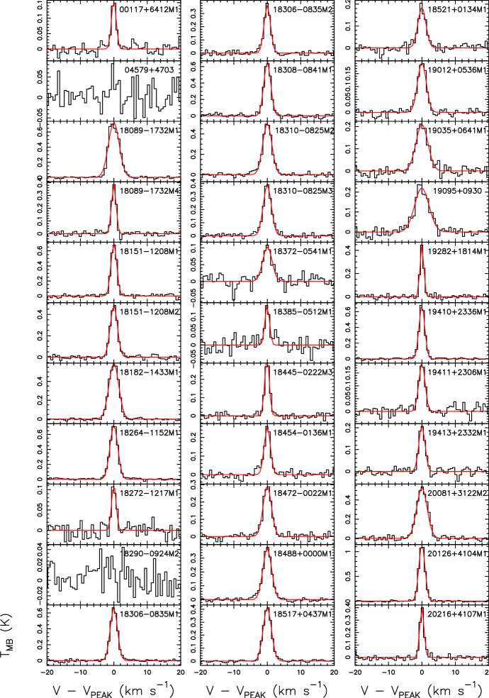
Figure 7: Spectra of HN¹³C(1-0) obtained for the sources. For each spectrum the x-axis represents a velocity interval of $\pm 20$ km s^-1 around the velocity listed in the second column of Table LABEL:fit1. The y-axis shows the intensity in main beam temperature units. The red curves are the best Gaussian fits obtained with MADCUBA.

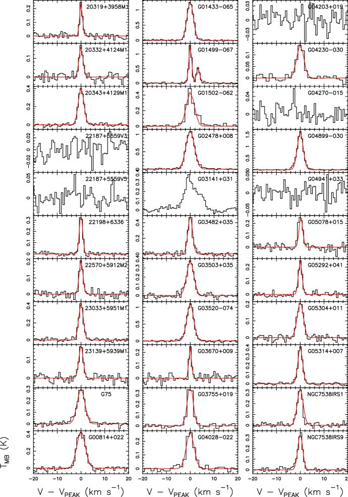
Figure 8: Fig. 7 continued. Note that for the source G01499-067 we have observed two components: we have fitted both lines and we have used both to compute the column densities.

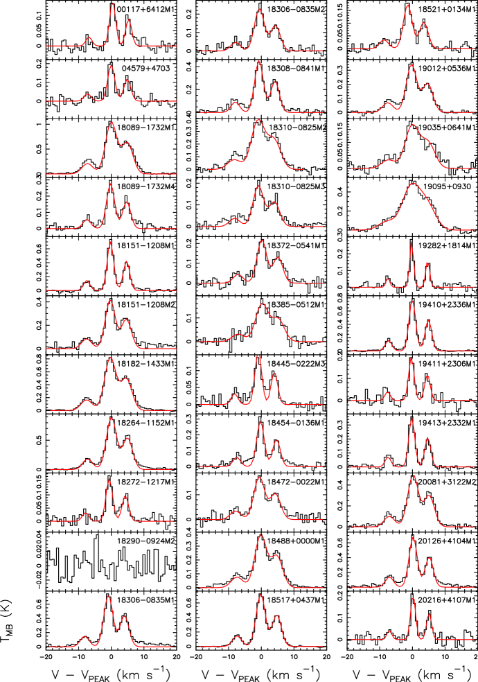
Figure 9: Spectra of H¹³CN(1-0) obtained for the sources. For each spectrum the x-axis represents a velocity interval of $\pm 20$ km s^-1 around the velocity listed in the second column of Table LABEL:fit2. The y-axis shows the intensity in main beam temperature units. The red curves are the best Gaussian fits obtained with MADCUBA.

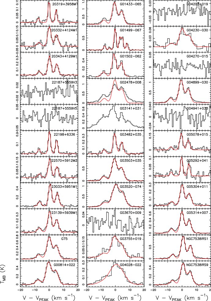
Figure 10: Fig. 9 continued. Note that for the source G01499-067 we have observed two components: we have fitted both lines and we have used both to compute the column densities.

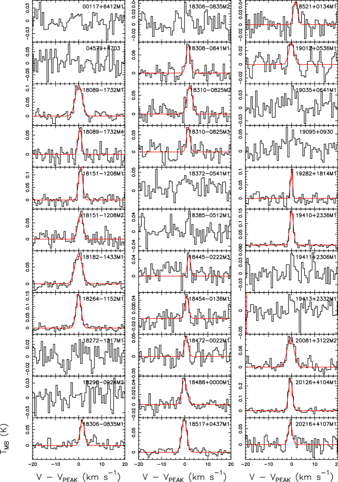
Figure 11: Spectra of H¹⁵NC(1-0) obtained for the sources. For each spectrum the x-axis represents a velocity interval of $\pm 20$ km s^-1 around the velocity listed in the second column of Table LABEL:fit1. The y-axis shows the intensity in main beam temperature units. The red curves are the best Gaussian fits obtained with MADCUBA.

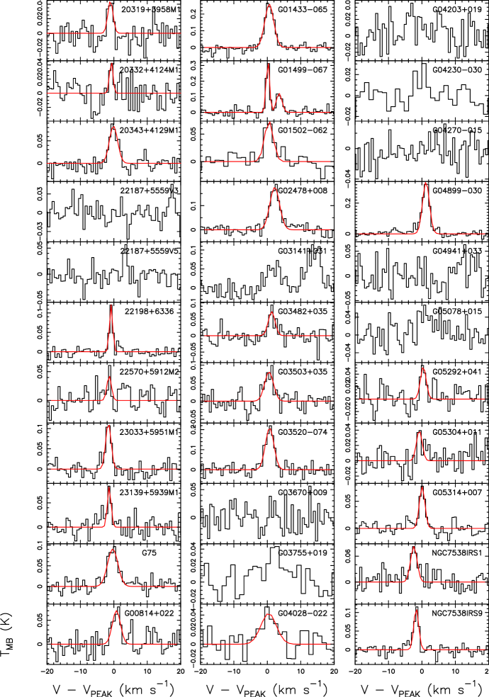
Figure 12: Continue of Fig. 11. Note that for the source G01499-067 we have observed two components: we have fitted both lines and we have used both to compute the column densities.

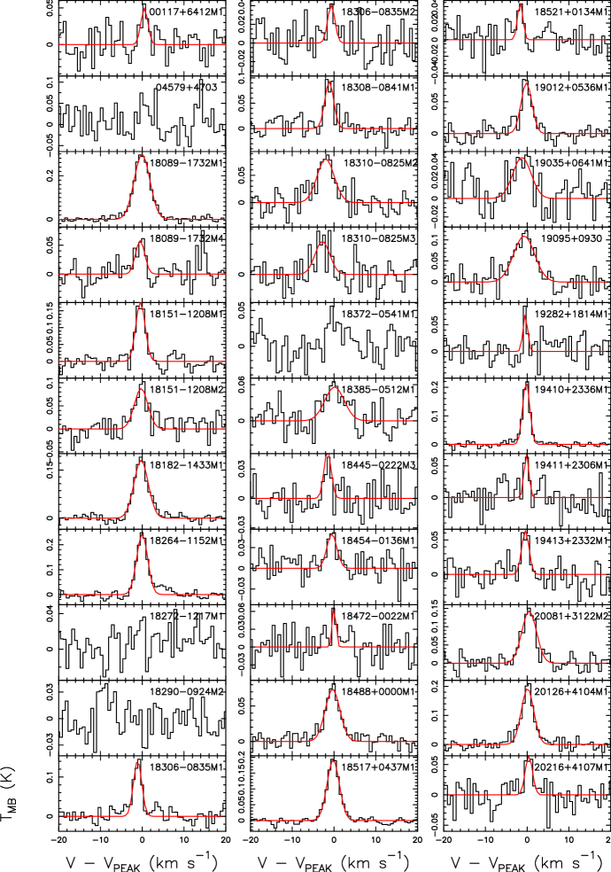
Figure 13: Spectra of HC¹⁵N(1-0) obtained for the sources. For each spectrum the x-axis represents a velocity interval of $\pm 20$ km s^-1 around the velocity listed in the second column of Table LABEL:fit2. The y-axis shows the intensity in main beam temperature units. The red curves are the best Gaussian fits obtained with MADCUBA.

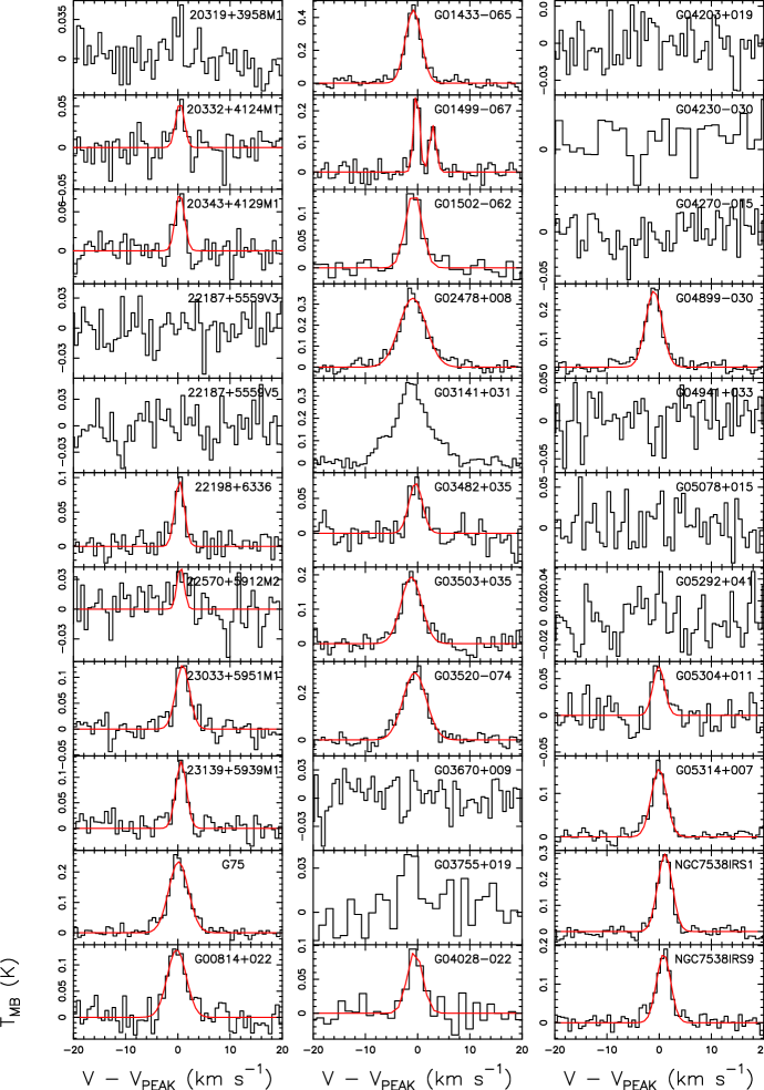
Figure 14: Continue of Fig. 13. Note that for the source G01499-067 we have observed two components: we have fitted both lines and we have used both to compute the column densities.

References

- Adande (2012) Adande, G. R., & Ziurys, L. M. 2012, ApJ, 744, 194
- Araya (2005) Araya, E., Hofner, P., Kurtz, S., Bronfman, L., & DeDeo, S. 2005, ApJS, 157, 279
- Beltran (2004) Beltrán, M. T., Cesaroni, R., Neri, R., et al. 2004, ApJL, 601, L187
- Beltran (2005) Beltrán, M. T., Cesaroni, R., Neri, R., et al. 2005, A&A, 435, 901
- Beltran (2016) Beltrán M. T., de Wit W. J., 2016, A&ARv, 24, 6
- Beltran (2018) Beltrán, M. T., Cesaroni, R., Rivilla, V. M., Sánchez-Monge, Á., Moscadelli, L., et al., 2018, arXiv:1803.05300
- Beuther (2002) Beuther, H., Schilke, P., Menten, K. M., et al. 2002, ApJ, 566, 945
- Bizzocchi (2013) Bizzocchi, L., Caselli, P., Leonardo, E., & Dore, L. 2013, A&A, 555, AA109
- Bockelee-Morvan (2008) Bockelée-Morvan, D., Biver, N., Jehin, E., et al. 2008, ApJ, 679, L49
- Caselli & Ceccarelli (2012) Caselli, P., & Ceccarelli, C. 2012, A&ARv, 20, 56
- Cazzoli (2005) Cazzoli, G., Puzzarini, C., & Gauss, J. 2005, ApJS, 159, 181
- Cazzoli (2005) Cazzoli, G., & Puzzarini, C., 2005, J. Mol. Spectrosc. 233, 280
- Cesaroni (2011) Cesaroni, R., Beltrán, M. T., Zhang, Q., Beuther, H., & Fallscheer, C. 2011, A&A, 533, A73
- Cesaroni (2017) Cesaroni, R., Sánchez-Monge, Á, Beltrán, M. T., et al. 2017, A&A, 602, A59
- Chin (1999) Chin, Y.-N., Henkel C., Langer N., & Mauersberger R. 1999, ApJ, 512, L143
- Clayton (2003) Clayton, D. D. 2003, Handbook of Isotopes in the Cosmos: Hydrogen to Gallium (Cambridge: Cambridge Univ. Press)
- Colzi (2018) Colzi, L., Fontani F., Caselli P., Ceccarelli C., Hily-Blant P., Bizzocchi L., 2018, A&A 609, A129
- Dahmen (1995) Dahmen, G.; Wilson, T. L.; Matteucci, F. 1995, A&A, 295, 194
- Daniel et al. (2013) Daniel, F., Gérin, M., Roueff, E., et al. 2013, A&A, 560, A3
- Daniel et al. (2016) Daniel F. et al., 2016, A&A, 592, A45
- Fontani et al. (2011) Fontani, F., Palau, Aina, Caselli, P., Sánchez-Monge, Á., Butler, M.J., et al. 2011, A&A, 529, L7
- Fontani et al. (2015a) Fontani, F., Caselli, P., Palau, Aina, Bizzocchi, L, Ceccarelli, C. 2015a, ApJ, 808, L46
- Gerin (2009) Gerin M, Marcelino N, Biver N, Roueff E, Coudert LH, et al. 2009. Astron. Astrophys. 498:L9–L12
- Guzman (2017) Guzmán, V. V., Öberg, K. I., Huang, J., Loomis, R., Qi, C. 2017, ApJ, 836, article id. 30, 15 pp
- Hily-Blant et al. (2013a) Hily-Blant, P., Pineau des Forets, G., Faure, A., Le Gal, R., Padovani, M. 2013, A&A, 557, 65
- Hily-Blant et al. (2017) Hily-Blant, P., Magalhaes, V., Kastner, J., Faure, A., Forveille, T., Qi, C. 2017, A&A 603, L6
- Izzard et al. (2004) Izzard, R.G., Tout, C.A., Karakas, A.I., Pols, O.R. 2004, MNRAS, 350, 407
- Kahane (2018) Kahane, C., Al-Edhari, A. J., Ceccarelli, C., Lopez-Sepulcre, A., Fontani, F., Mihkel, K., 2018, ApJ, 825, 130
- Kelly (2007) Kelly, B. C. 2007, ApJ, 665, 1489
- Klein (2012) Klein B., Hochgürtel S., Krämer I., Bell A., Meyer K., Güsten R., 2012, A&A, 542, L3
- vanKooten (2017) van Kooten, E. M. M. E.; Nagashima, K.; Kasama, T.; Wampfler, S. F.; Ramsey, J. P.; Frimann, S.; Balogh, Z. I.; Schiller, M.; Wielandt, D. P.; Franchi, I. A.; Jørgensen, J. K.; Krot, A. N.; Bizzarro, M., 2017, Geochimica et Cosmochimica Acta, Volume 205, p. 119-148
- Lis (2010) Lis DC, Phillips TG, Goldsmith PF, Neufeld DA, Herbst E, et al. 2010a. Astron. Astrophys. 521:L26
- Maciel (2009) Maciel, W. J., & Costa, R. D. D. 2009, in IAU Symp. 265, Chemical Abundances in the Universe: Connecting First Stars to Planets, Vol. 5, ed. K. Cunha, M. Spite, & B. Barbuy (Cambridge: Cambridge Univ. Press), 317
- Manfroid (2009) Manfroid, J., Jehin, E., Hutsemékers, D., et al.: The CN isotopic ratios in comets. A&A, 503, 613-624(2009)
- Marty (2009) Marty, B., Zimmermann, L., Burnard, P.G.: Geochimica et Cosmochimica Acta73, 842(2009)
- Marty (2010) Marty, B., Zimmermann, L., Burnard, P.G., Wieler, R., et al.: Geochimica et Cosmochimica Acta74, 340-355(2010)
- Meibom (2007) Meibom, A., Krot, A. N., Robert, F., et al. 2007, ApJ, 656, L33
- Milam (2005) Milam, S.N., Savage, C,m Brewster, M.A., Ziurys, L.M., Wyckoff, S. 2005, Ap.J., 634, 1126
- Muller (2011) Muller, S., Beelen, A., Guélin, M., et al. 2011, A&A, 535, A103
- Nomoto (2013) Nomoto K., Kobayashi C., Tominaga N., 2013, ARA&A, 51, 457
- Padovani (2011) Padovani, M., Walmsley, C. M., Tafalla, M., Hily-Blant, P., & Pineau Des Forêts, G. 2011, A&A, 534, A77
- Pearson (1976) Pearson, E. F., Creswell, R. A., Winnewisser, M., & Winnewisser, G. 1976, ZNatA, 31a, 1394
- Pety (2005) Pety, J. 2005, in SF2A-2005: Semaine de l’Astrophysique Francaise, ed. F. Casoli, T. Contini, J. M. Hameury, & L. Pagani, 721
- Purcell (2006) Purcell, C. R., Balasubramanyam, R., Burton, M. G., et al. 2006, MNRAS, 367, 553
- Reid (2009) Reid, M. J., Menten, K. M., Zheng, X. W., et al. 2009, ApJ, 700, 137
- Reid (2014) Reid M. J. et al., 2014, ApJ, 783, 130
- Rivilla (2016) Rivilla V. M., Fontani F., Beltran M. T., Vasyunin A., Caselli P., Martín-Pintado J., Cesaroni R., 2016, ApJ, 826, 161
- Rivilla (2017) Rivilla, V. M., Beltrán, M. T., Cesaroni, R., et al. 2017, A&A, 598, A59
- Romano (2003) Romano, D., & Matteucci, F. 2003, MNRAS, 342, 185
- Romano (2017) Romano, D., Matteucci, F., Zhang, Z.-Y., Papadopoulos, P.P., Ivison, R.J. 2017, MNRAS, 470, 401
- Roueff et al. (2015) Roueff, E., Loison, J.C., Hickson, K.M. 2015, A&A, 576, 99
- Schmitt (2002) Schmitt, J.H.M.M., & Ness, J.-U. 2002, A&A, 388, L13
- vanderTak (2009) van der Tak, F. F. S., Müller, H. S. P., Harding, M. E., & Gauss, J. 2009, A&A, 507, 347
- Sridharan (2002) Sridharan, T. K., Beuther, H., Schilke, P., Menten, K. M., & Wyrowski, F. 2002, ApJ , 566, 931
- Tan (2014) Tan J. C., Beltran M. T., Caselli P., Fontani F., Fuente A., Krumholz M. R., McKee C. F., Stolte A., 2014, Protostars and Planets VI, p. 149
- wallstrom (2016) Wallström S. H. J., Muller S., Guélin M., 2016, A&A, 595, A96
- Wampfler (2014) Wampfler, S. F., Jørgensen, J. K., Bizzarro, M., & Bisschop, S. E. 2014, A&A, 572, A24
- Wang et al. (2014) Wang, J., Zhang, Z.-Y., Qiu, J., Shi, Y., Zhang, J., Fang, M. 2014, ApJ, 796, 57
- Wirström et al. (2012) Wirström, E. S., Charnley, S. B., Cordiner, M. A., & Milam, S. N. 2012, ApJL, 757, L11
- Wouterloot (1993) Wouterloot J. G. A., Brand J., Fiegle K., 1993, A&AS, 98, 589
- Zapata (2013) Zapata, L. A., Loinard, L., Rodríguez, L. F., et al. 2013, ApJL, 764, L14
- Zeng (2017) Zeng, S., Jimenez-Serra, I., Cosentino, G., Viti, S., Barnes, A. T., Henshaw, J. D., Caselli, P., Fontani, F., Hily-Blant, P., 2017, A&A, 603, A22