Enrich-by-need Protocol Analysis for Diffie-Hellman
(Extended version)

Abstract

Enrich-by-need protocol analysis is a style of symbolic protocol analysis that characterizes all executions of a protocol that extend a given scenario. In effect, it computes a strongest security goal the protocol achieves in that scenario. cpsa, a Cryptographic Protocol Shapes Analyzer, implements enrich-by-need protocol analysis.

In this paper, we describe how to analyze protocols using the Diffie-Hellman mechanism for key agreement (DH) in the enrich-by-need style. DH, while widespread, has been challenging for protocol analysis because of its algebraic structure. DH essentially involves fields and cyclic groups, which do not fit the standard foundational framework of symbolic protocol analysis. By contrast, we justify our analysis via an algebraically natural model.

This foundation makes the extended cpsa implementation reliable. Moreover, it provides informative and efficient results.

An appendix, written by John Ramsdell in 2014, explains how unification is efficiently done in our framework.

1 Introduction

Diffie-Hellman key agreement (DH) [9], while widely used, has been challenging for mechanized security protocol analysis. Some techniques, e.g. [13, 8, 30, 23], have produced informative results, but focus only on proving or disproving individual protocol security goals. A protocol and a specific protocol goal are given as inputs. If the tool terminates, it either proves that this goal is achieved, or else provides a counterexample. However, constructing the right security goals for a protocol requires a high level of expertise.

By contrast, the enrich-by-need approach starts from a protocol and some scenario of interest. For instance, if the initiator has had a local session, with a peer whose long-term secret is uncompromised, what other local sessions have occurred? What session parameters must they agree on? Must they have happened recently, or could they be stale?

Enrich-by-need protocol analysis identifies all essentially different smallest executions compatible with the scenario of interest. While there are infinitely many possible executions—since we put no bound on the number of local sessions—often surprisingly few of them are really different. The Cryptographic Protocol Shapes Analyzer (cpsa) [35], a symbolic protocol analysis tool based on strand spaces [40, 16, 25], efficiently enumerates these minimal, essentially different executions. We call the minimal, essentially different executions the protocol’s shapes for the given scenario.

Knowing the shapes tells us a strongest relevant security goal, i.e. a formula that expresses authentication and confidentiality trace properties, and is at least as strong as any one the protocol achieves in that scenario [18, 34]. Using these shapes, one can resolve specific protocol goals. The hypothesis of a proposed security goal tells us what scenario to consider, after which we can simply check whether the conclusion holds in each resulting shape (see [37] for a precise logical treatment).

Moreover, enrich-by-need has key advantages. Because it can also compute strongest goal formulas directly for different protocols, it allows comparing the strength of different protocols [37], for instance during standardization. Moreover, the shapes provide the designer with visualizations of exactly what the protocol may do in the presence of an adversary. Thus, they make protocol analysis more widely accessible, being informative even for those whose expertise is not mechanized protocol analysis.

In this paper, we show how we strengthened cpsa’s enrich-by-need analysis to handle DH. It is efficient, and has a flexible adversary model with corruptions.

Foundational issues needed to be resolved. For one thing, finding solutions to equations in the natural underlying theories is undecidable in general, which means that mechanized techniques must be carefully circumscribed. For another, these theories, which include fields, are different from many others in security protocol analysis. The field axioms are not (conditional) equations, meaning that they do not have a simplest (or “initial”) model for the analysis to work within. Much work on mechanized protocol analysis, even for DH, which relies on equational theories and their initial models, e.g. [13, 8, 30, 23]. However, one would like an analysis method to have an explicit theory justifying it relative to the standard mathematical structures such as fields. cpsa now has a transparent foundation in the algebraic properties of the fields that DH manipulates. This development extends our earlier work [12, 24].

Contributions.

In this paper, we describe how we extended cpsa to analyze DH protocols. Our method is currently restricted to protocols that do not use addition in the exponents, which is a large class. We call these multiplicative protocols. The method is also restricted to protocols that disclose randomly chosen exponents one-by-one. This allows modeling a wide range of possible types of corruption; however, it excludes a few protocols in which products of exponents are disclosed. We say that a protocol separates disclosures if it satisfies our condition.

cpsa’s analysis is based on two principles—Lemmas 4 and 5—that are valid for all executions of a protocol $\Pi$, if $\Pi$ is multiplicative and separates disclosures. They characterize how the adversary can obtain an exponent value such as $xy$ or an exponentiated DH value such as $g^{xy}$, resp. They tell cpsa what information to add to a partial analysis to get one or more possible enrichments that describe the different executions in which the adversary obtains these values. Lemmas 11–12 show how cpsa represents the enrichments.

To formulate and prove these lemmas, we had to clarify the algebraic structures we work with. In our semantics, the messages in protocol executions contain mathematical objects such as elements of fields and cyclic groups. We regard the the random choices of the compliant protocol participants serve as “transcendentals,” i.e. primitive elements added to a base field that have no algebraic relationship to members of the base field. The adversary cannot rely on any particular algebraic relations with known values before the compliant participant has made the random choice. Even after the choice of a value $x$, if the adversary sees only the exponentiated value $g^{x}$, the adversary still does not know any algebraic (polynomial) constraints on $x$. Instead, as in the Generic Group Model [39, 29], the adversary can apply algebraic operations to such values, but cannot benefit from the bitstrings by means of which they are represented.

cpsa’s analysis operates within a language of first order predicate logic. The analysis relates to real protocol executions via Tarski-style satisfaction. Protocol executions (using group and field elements as messages, in the presence of an adversary) are the models of the theories used in the analysis process. This provides a familiar foundational setting.

cpsa is very efficient. When executed on a rich set of variants of Internet Key Exchange (IKE) versions 1 and 2, our analysis required less than 30 seconds on a laptop. By contrast, Scyther analyzed this same set of IKE variants, requiring about a day of work on a computing cluster [7]. This is about 3.4 orders of magnitude more time, quite apart from the difference between the quite powerful cluster (circa 2010) and the laptop (built circa 2015). Another benchmark [4] with little use of DH led to similar results. This suggests that cpsa is broadly efficient, with or without DH. Performance data for Tamarin and Maude-NPA is less available.

2 An example: Unified Model

Many variants of the original Diffie-Hellman idea [9] exchange both certified, long-term values $g^{a}$ and $g^{b}$, and also one-time, ephemeral values $g^{x}$ and $g^{y}$. The peers agree compute session keys using key computation functions $\mathsf{KCF}^{(\cdot)}$, where in successful sessions, $\mathsf{KCF^{A}}(a,x,g^{b},g^{y})=\mathsf{KCF^{B}}(b,y,g^{a},g^{x})$. The ephemeral values ensure the two parties agree on a different key in each session. The long-term values are intended for authentication, namely that any party that obtains the session key must be one of the intended peers. Different functions $\mathsf{KCF}^{(\cdot)}$ yield different security properties. Protocol analysis tools for DH key exchanges must be able to use algebraic properties to identify these security consequences.

2.1 DH Challenge-Response with Unified Model keying

We consider here a simple DH Challenge-Response protocol ${\mathsf{DHCR}}$ in which nonces from each party form a challenge and response protected by a shared, derived DH key (see Fig. 1).

where	init computes $K$ as	$\mathsf{KCF^{A}}({a},x,g^{b},g^{\beta})$
	resp computes $K$ as	$\mathsf{KCF^{B}}({b},y,g^{{a}},g^{\alpha})$

Figure 1: Protocol ${\mathsf{DHCR}}$: Initiator, responder, and $\mathsf{ltx}()$ self-certifying roles. The $\mathtt{certs}$ are $[\![\,g^{\mathsf{ltx}(A)}\,]\!]_{\mathsf{sk}(P)}$ and $[\![\,g^{\mathsf{ltx}(B)}\,]\!]_{\mathsf{sk}(P)}$ for each role.

Each participant obtains two self-signed certificates, covering the long term public values of his peer and himself. $A$ and $B$’s long-term DH exponents are values $\mathsf{ltx}(A),\mathsf{ltx}(B)$, which we will mainly write as a lower case $a,b$. We assume that the principals are in bijection with distinct long-term $\mathsf{ltx}(\cdot)$ values.

Each participant furnishes an ephemeral public DH value $g^{x},g^{y}$ in cleartext, and also a nonce. Each participant receives a value which may be the peer’s ephemeral, or may instead be some value selected by an active adversary. Neither participant can determine the exponent for the ephemeral value he receives, but since the value is a group element, it must be some value of the form $g^{\alpha},g^{\beta}$.

Each participant computes a session key using his $\mathsf{KCF}^{(\cdot)}$. The responder uses the key to encrypt the nonce received together with his own nonce. The initiator uses the key to decrypt this package, and to retransmit the responder’s nonce in plaintext as a confirmation.

The registration role allows any principal $P$ to emit its long-term public group value $g^{\mathsf{ltx}(P)}$ under its own digital signature. In full-scale protocols, a certifying authority’s signature would be used, but in this example omit the CA so as not to distract from the core DH issues.

We will assume that each instance of a role chooses its values for certain parameters freshly. For instance, each instance of the registration role makes a fresh choice of ${\mathsf{ltx}(P)}$. Each instance of the initiator role chooses $x$ and $na$ freshly, and each responder instance chooses $y$ and $nb$ freshly.

This protocol is parameterized by the key computations. We consider three key computations from the Unified Model [1], with a hash function $\#(\cdot)$ standing for key derivation. The shared keys—when each participant receives the ephemeral value $g^{\alpha}=g^{x}$ or $g^{\beta}=g^{y}$ that the peer sent—are:

Plain UM:	$\#(g^{{a}{b}},g^{xy})$;
Criss-cross UMX:	$\#(g^{{a}y},g^{{b}x})$;
Three-component UM3:	$\#(g^{{a}y},g^{{b}x},g^{xy})$

We discuss three security properties:

Authentication:

If either the initiator or responder completes the protocol, and both principals’ private long-term exponents are secret, then the intended peer must have participated in a matching conversation.

All three key computations UM, UMX, and UM3 enforce the authentication goal.

Impersonation resistance:

If either the initiator or responder completes the protocol, and the intended peer’s private long-term exponent is secret, then the intended peer must have participated in a matching conversation.

Here we do not assume that ones own private long-term exponent is secret. Can the adversary impersonate the intended peer if ones own key is compromised?

${\mathsf{DHCR}}$ with the plain UM KCF is susceptible to an impersonation attack: An attacker who knows Alice’s own long-term exponent can impersonate any partner to Alice. The adversary can calculate $g^{{a}{b}}$ from ${a}$ and $g^{{b}}$, and can calculate the $g^{xy}$ value from $g^{x}$ and a $y$ it chooses itself.

On the other hand, the UMX and UM3 KCFs resist the impersonation attack.

Forward secrecy:

If the intended peers complete a protocol session and then the private, long-term exponent of each party is exposed subsequently, then the adversary still cannot derive the session key.

This is sometimes called weak forward secrecy.

To express forward secrecy, we allow the registration role to continue and subsequently disclose the long term secret $\mathsf{ltx}(P)$ as in Fig. 2. If we assume in an analysis that $\mathsf{ltx}(P)$ is uncompromised, that implies that this role does not complete.

Figure 2: The registration role in full

The dummy second node allows specifying that the $\mathsf{ltx}(P)$ release node occurs after some other event, generally the completion of a normal session.

The Normal UM KCF guarantees forward secrecy, but UMX does not. In UMX, if an adversary records both $g^{x}$ and $g^{y}$ during the protocol and learns ${a}$ and ${b}$ later, the adversary can compute the key by exponentiating $g^{x}$ to the power $b$ and $g^{y}$ to the power $a$.

UM3 restores forward secrecy. It meets all three goals.

2.2 Strand terminology

In discussing how cpsa carries out its analysis, we will use a small amount of the strand space terminology; see Section 4 for more detail.

We call a sequence of transmission and reception events as illustrated in Figs. 1–2 a strand. We call each send-event or receive-event on a strand a node. We draw strands either horizontally as in Figs. 1–2 or vertically, as in diagrams generated by cpsa itself.

A protocol consists of a finite set of these strands, which we call the roles of the protocol. The roles contain variables, called the parameters of the roles, and by plugging in values for the parameters, we obtain a set of strands called the instances of the roles. We also call a strand a regular strand when it is an instance of a role, because it then complies with the rules. Regular nodes are the nodes that lie on regular strands. We speak of a regular principal associated with a secret if that secret is used only in accordance with the protocol, i.e. only in regular strands.

In an execution, events are (at least) partially ordered, and values sent on earlier transmissions are available to the adversary, who would like to provide the messages expected by the regular participants on later transmission nodes. The adversary can also generate primitive values on his own. We will make assumptions restricting which values the adversary does generate to express various scenarios and security goals.

2.3 How CPSA works, I: UMX initiator

Here we will illustrate the main steps that cpsa takes when analyzing $\mathsf{DHCR}$. For this illustration, we will focus on the impersonation resistance of the UMX key computation, in the case where the initiator role runs, aiming to ensure that the responder has also taken at least the first three steps of a matching run. The last step of the responder is a reception, so the initiator can never infer that it has occurred. We choose this case because it is typical, yet quite compact.

Starting point.

We start cpsa on the problem shown in Fig. 3,

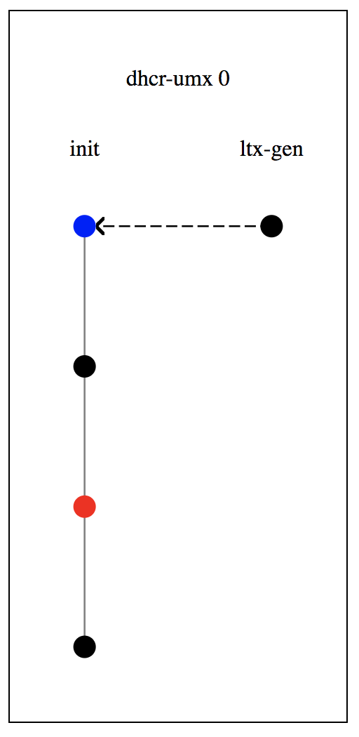
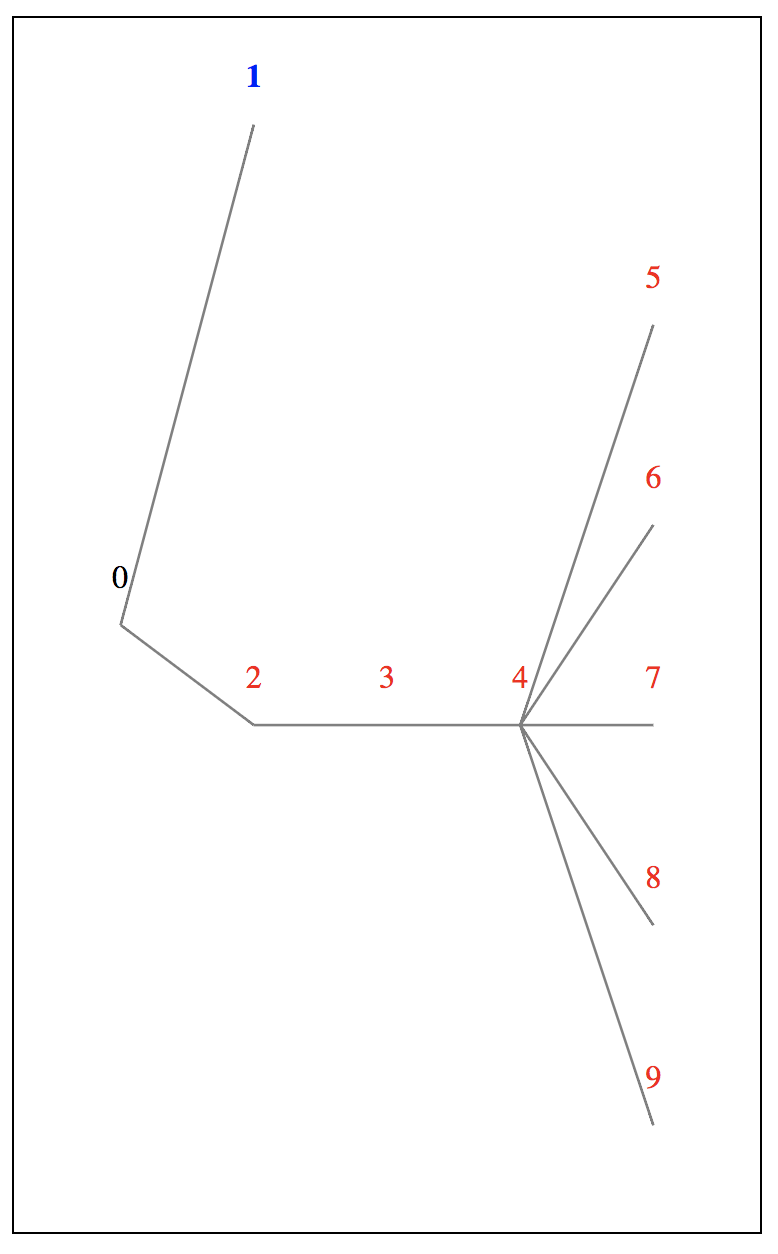
Figure 3: Skeleton 0: The initial scenario, assuming $\mathsf{ltx}(B)$ non-compromised and $A\not=B$.  cpsa exploration tree

in which $A$, playing the initiator role, has made a full local run of the protocol, and received the long term public value of $B$ from a genuine run of the ltx-gen role. These are shown as the vertical column on the left and the single transmission node at the top to its right. We will assume that $B$’s private value $\mathsf{ltx}(B)$ is non-compromised and freshly generated, so that the public value $g^{\mathsf{ltx}(B)}$ originates only at this point. In particular, this run definitely does not progress to expose the secret as in the third node of Fig. 2. The fresh selection of $\mathsf{ltx}(B)$ must certainly precede the reception of $g^{\mathsf{ltx}(B)}$ at the beginning of the initiator’s run. This is the meaning of the dashed arrow between them. We do not assume that $A$’s long term secret ${\mathsf{ltx}(A)}$ is uncompromised, although we will assume that the ephemeral $x$ value is freshly generated by the initiator run, and not available to the adversary. We assume $A\not=B$, which is the case of most interest.

Exploration tree.

In Fig. 3, we also show the exploration tree that cpsa generates. Each item in the tree—we will call each item a skeleton—is a scenario describing some behavior of the regular protocol participants, as well as some assumptions. For instance, skeleton 0 contains the assumptions about ${\mathsf{ltx}(B)}$ and $A$’s ephemeral value $x$ mentioned before. The exploration tree contains one blue, bold face entry, skeleton 1 (shown in Fig. 4), as well as a subtree starting from 2 that is all red. The bold blue skeleton 1 is a shape, meaning it describes a simplest possible execution that satisfies the starting skeleton 0. The red skeletons are dead skeletons, meaning possibilities that the search has excluded; no executions can occur that satisfy these skeletons. Thus, skeleton 1 is the only shape, and cpsa has concluded that all executions that satisfy skeleton 0 in fact also satisfy skeleton 1.

In other examples, there may be several shapes identified by the analysis, or in fact zero shapes. The latter means that the initial scenario cannot occur in any execution. This may be the desired outcome, for instance when the initial scenario exhibits some disclosure that the protocol designer would like to ensure is prevented.

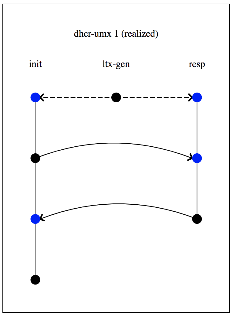
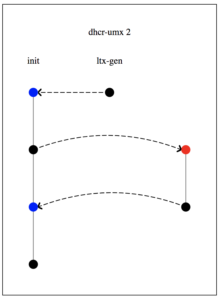
Figure 4: Skeleton 1, the sole resulting shape.  Skeleton 2: Can the UMX encryption key $K$ be exposed, on the rightmost strand?

First step.

cpsa, starting with skeleton 0 in Fig. 3, identifies the third node of the initiator strand, which is shown in red, as unexplained. This is the initiator receiving the DH ephemeral public value $g^{y}$ and the encryption $\{\!|na,nb|\!\}_{K}$, where $K$ is the session key $A$ computes using $g^{y}$ and the other parameters. The node is red because the adversary cannot supply this message on his own, given the materials we already know that the regular, compliant principals have transmitted. Thus, cpsa is looking for additional information, including other transmissions of regular participants, that could explain it. Two possibilities are relevant here, and they lead to skeletons 1 and 2 (see Fig. 4).

In skeleton 1, a regular protocol participant executing the responder role transmits the message $g^{y},\{\!|na,nb|\!\}_{K}$. Given the values in this message—including those used to compute $K$ using the UMX function—all of the parameters in the responder role are determined. It is executed by the intended peer $B$, who is preparing the message for $A$, with matching values for the nonces and ephemeral exponents. These are matching conversations [5, 27]. A solid arrow from one node to another means that the former precedes the latter, and moreover it transmits the same message that the latter receives.

Skeleton 2 considers whether the key $K=\#(g^{ay},g^{bx})$, computed by the initiator, might be compromised. $K$ is the value received on the rightmost strand. The reception node is called a listener node, because it witnesses for the availability of $K$ to the adversary. The “heard” value $K$ is then retransmitted so that cpsa can register that this event must occur before the initiator’s third node. This listener node is red because cpsa cannot yet explain how $K$ would become available. However, if additional information, such as more actions of the regular participants, would explain it, then the adversary could use $K$ to encrypt $na,nb$ and forge the value $A$ receives. Thus, skeleton 2 identifies this listener node for further exploration.

Step 2.

Proceeding from skeleton 2, cpsa performs a simplification on $K=\#(g^{ay},g^{bx})$. The value $y$ is available to the adversary, as is $a$, since we have not assumed them uncompromised. Thus, $g^{ay}$ is available. The adversary will be able to compute $K$ if he can obtain $g^{bx}$. Skeleton 3 (not shown) is similar to skeleton 2 but has a red node asking cpsa to explain how to obtain $g^{bx}$.

This requires a step which is distinctive to DH protocols. cpsa adds Skeleton 4, which has a new rightmost strand with a red node, receiving the pair $g^{bx/w},w$. To resolve this, cpsa must meet two constraints. First, it must choose an exponent $w$ that can be exposed and available to the adversary. Second, for this value of $w$, either $w=bx$ or else the “leftover” DH value $g^{bx/w}$ must be transmitted by a regular participant and extracted by the adversary.

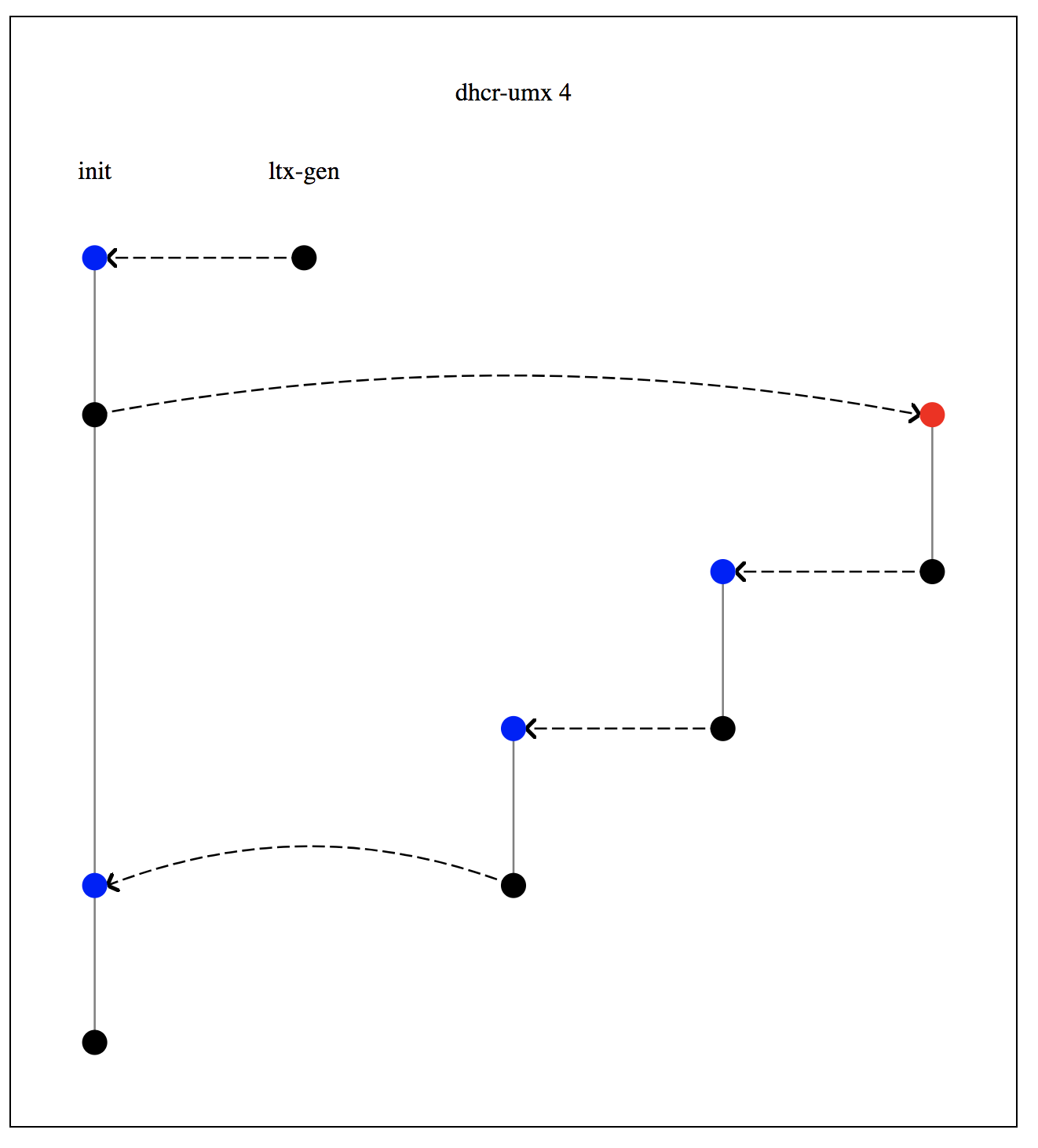
Figure 5: Skeleton 4: $g^{bx/w},w$ is on the rightmost strand. Is there an exposed exponent $w$ where either $w=bx$ or else $g^{bx/w}$ was sent by a regular participant?

One of our key lemmas, Lemma 5, justifies this step.

Step 3, clean-up.

From skeleton 4, cpsa considers the remaining possibilities in this branch of its analysis. First, it immediately eliminates the possibility $w=bx$, since the protocol offers no way for the adversary to obtain $b$ and $x$.

In fact, because $b$ and $x$ are random values, independently chosen by different principals, the adversary cannot obtain their product without obtaining the values themselves.

cpsa then considers each protocol role in turn, namely the initiator, responder, and registration roles. Can any role transmit a DH value of the form $g^{bx/w}$, where the resulting inferred value for $w$ would be available to the adversary?

In skeleton 5, it considers the case in which the initiator strand is the original starting strand, which transmits $g^{x}$. Thus, $x=bx/w$, which is to say $w=b$. However, since $b$ is assumed uncompromised, the adversary cannot obtain it, and this branch is dead. Skeleton 6 explores the case where a different initiator strand sends $g^{z}$, so $z=bx/w$, i.e. $w=bx/z$. However, this is unobtainable, since it too is compounded from independent, uncompromised values $b,x,z$.

Skeleton 7 considers the responder case, and skeletons 8 and 9 consider a registration strand which is either identical with the initial one (skeleton 8) or not (skeleton 9). They are eliminated for corresponding reasons.

The entire analysis takes about 0.2 second.

CPSA overall algorithm.

In this paper, unlike earlier work, a skeleton for $\Pi$ will be a theory that a set of executions satisfies. This may be the empty set of executions, in which case the skeleton is “dead,” like skeletons 2–9.

Protocol analysis in cpsa starts with a skeleton, the initial scenario. At any step, cpsa has a set $\mathcal{S}$ of skeletons available. If $\mathcal{S}$ is empty, the run is complete.

Otherwise, cpsa selects a skeleton $\mathbb{A}$ from $\mathcal{S}$. If $\mathbb{A}$ is realized, meaning that it gives a full description of some execution, then cpsa records it as a result. Otherwise, there is some reception node $n$ within $\mathbb{A}$ that is not explained. This $n$ is the target node. That means that cpsa cannot show how the message received by $n$ could be available, given the actions the adversary can perform on his own, or using messages received from earlier transmissions.

cpsa replaces $\mathbb{A}$ with a “cohort.” This is a set $\mathbb{C}_{1},\ldots,\mathbb{C}_{k}$ of extensions of the theory $\mathbb{A}$. For every execution satisfying $\mathbb{A}$, there should be at least one of the $\mathbb{C}_{i}$ which this execution satisfies. cpsa must not “lose” executions. When $k=0$ and there are no cohort members, cpsa has recognized that $\mathbb{A}$ is dead. cpsa then repeats this process starting with $\mathcal{S}\setminus\{\mathbb{A}\}\cup\{\mathbb{C}_{1},\ldots,\mathbb{C}_{k}\}$.

CPSA cohort selection.

cpsa generates its cohorts by adding one or more facts, or new equalities, to $\mathbb{A}$, to generate each $\mathbb{C}_{i}$. It also does some renaming, so that the theories $\mathbb{C}_{i}$ result from a theory interpretation from $\mathbb{A}$ rather than syntactic extension.

The selection of facts to add is based on a taxonomy of the executions satisfying $\mathbb{A}$. In each one of them, the reception on the target node $n$ must somehow be explained. There are only a limited number of types of explanation, which are summarized in Fig. 6.

  

Regular transmission:

Some principal, acting in accordance with the protocol (i.e. “regularly”), has transmitted a message in this execution which is not described in $\mathbb{A}$.

Skeleton 1 was introduced in this way in step 1 above.

Encryption key available:

An encrypted value in a reception must be explained, and the adversary obtains the encryption key in a way that cpsa will subsequently explore.

Skeleton 2 was introduced in this way in step 1 above.

Decryption key available:

A value was previously transmitted in encrypted form, and, in a way that cpsa will subsequently explore, the adversary obtains the decryption key to extract it.

Specialization:

The execution satisfies additional equations, not included in $\mathbb{A}$, and in this special case the adversary can obtain the target node message.

DH value computed:

The adversary needs to supply a DH value $g^{\alpha}$, and obtains it from $g^{\alpha/w}$ by exponentiating with $w$, which must also be available.

Skeleton 4 was introduced in this way in step 2 above.

Exponent value computed:

The adversary must obtain an exponent $xw$. There are then two subcases:

1. Both $x$ and $w$ will be obtainable in ways that cpsa will subsequently explore; or

2. $w$ will be instantiated as some $v/x$, so that $x$ will cancel out. Thus, $x$ is in fact be absent from the instance of $xw$.

 

Figure 6: Kinds of cohort members.

Of these types, the first three are entirely unchanged. The Specialization clause is conceptually unchanged, but the unification algorithm that finds the relevant equations has been updated to reflect the DH algebra; it works efficiently in practice (see Section 4.3 below).

The last two clauses are new. Lemmas 5 and 4 justify them (resp.), and Cohort Cases 11 and 12 formulate how the skeletons $\mathbb{C}_{i}$ are defined from $\mathbb{A}$; in these cases they are in fact syntactic extensions. We will push the overall Theorem 2 into the Appendix (p. 2) to concentrate on these central cases.

We now briefly mention the types of step we have not yet illustrated.

A decryption step.

One must also handle a case dual to the encryption principle we used in step 1 above, leading from skeleton 0 to skeletons 1,2, but concerning decryption.

Consider the analysis from the responder’s point of view. In this scenario, the responder’s last step, in which he receives the decrypted nonce $nb$, needs explanation. The responder previously transmitted it inside the encryption in $g^{y},\{\!|na,nb|\!\}_{K}$. In this case, cpsa must explain the how $nb$ can escape from the protection of the encryption.

One possible explanation is that a regular transmission does so. That is, in some role of the protocol, a participant accepts messages of the form $\{\!|na,nb|\!\}_{K}$, and retransmits the second nonce outside this form. This is symmetric to the case with an initiator strand, leading to a shape very similar to skeleton 1.

The other possible explanation is that the adversary obtains the key $K=\#(g^{ay},g^{bx})$. This would allow the adversary to do the decryption, and free $nb$ from its protection. The analysis of the resulting skeleton 12 is almost identical with the analysis of skeleton 2 in Section 2.3.

A step for exponents.

When cpsa needs to explore the availability of some exponent value, such as $bx/z$ in an example above, it may be able to resolve the question directly. When it cannot, it takes a step based on our other key lemma, Lemma 4. This involves splitting the exploration tree, i.e. distinguishing possible cases. In one branch, variables will be instantiated so that an element such as $b$ in the exponent will be canceled out. The other branch explores whether the same element $b$ can be available to the adversary. cpsa resorts to this step relatively rarely when a protocol uses DH in straightforward ways; the forward secrecy analysis for the plain UM key computation gives an example however.

2.4 Performance

Our implementation of the cpsa tool is highly efficient. See Figure 7 for a list of performance results. We ran the tool not only on the Diffie-Hellman challenge-response protocol described in this section, with each of the key derivation options, but also on a rich set of variants of Internet Key Exchange (IKE) versions 1 and 2. Cremers’ Scyther tool was used circa 2010 to analyze this same set of variants [8]. The IKE variants were analyzed for an average of five properties each, yielding conclusions similar to those drawn using Scyther [8]. Scyther can thus be used as a basis for performance comparison. The authors reported that the analysis of the IKE variants took about a day of work on a computing cluster.

DHCR: Example & Time
dhcr-um   4.06s	dhcr-umx   0.72s	dhcr-um3   0.47s

IKEv1: Example & Time
IKEv1-pk2-a	1.06s	IKEv1-pk2-a2	1.02s
IKEv1-pk2-m	0.49s	IKEv1-pk2-m2	0.58s
IKEv1-pk-a1	1.27s	IKEv1-pk-a12	1.09s
IKEv1-pk-a2	1.00s	IKEv1-pk-a22	1.10s
IKEv1-pk-m	0.51s	IKEv1-pk-m2	0.49s
IKEv1-psk-a	0.43s	IKEv1-psk-m	0.68s
IKEv1-psk-m-perlman	0.69s	IKEv1-quick	0.66s
IKEv1-psk-quick-noid	0.65s	IKEv1-quick-nopfs	0.09s
IKEv1-sig-a1	0.15s	IKEv1-sig-a2	0.16s
IKEv1-sig-a-perlman	0.17s	IKEv1-sig-a-perlman2	0.19s
IKEv1-sig-m	0.21s	IKEv1-sig-m-perlman	0.19s
IKEv2: Example & Time
IKEv2-eap	1.35s	IKEv2-eap2	1.36s
IKEv2-mac	0.76s	IKEv2-mac2	0.97s
IKEv2-mac-to-sig	0.83s	IKEv2-mac-to-sig2	0.82s
IKEv2-sig	0.56s	IKEv2-sig2	0.54s
IKEv2-sig-to-mac	0.70s	IKEv2-sig-to-mac2	0.69s

Figure 7: cpsa Timings: DHCR-UM*, Internet Key Exchange v. 1 and 2.

In contrast, cpsa needed no more than 1.36 seconds to analyze any of the individual variants, and 21.32 seconds to analyze all of them combined. The data in Fig. 7 is from a run of cpsa on a mid-2015 MacBook Pro with a 4-core 2.2 GHz Intel Core i7 processor, run with up to 8 parallel threads using the Haskell run-time system.

Our analysis of the Diffie-Hellman challenge response protocol revealed the properties we expected, as described earlier in this section. Each cpsa run checked about five scenarios, considering the guarantees obtained by initiator and responder each under two sets of assumptions, as well as a forward secrecy property. Our analysis of the IKE variants discovered no novel attacks, but does sharpen Cremers’ analysis, because cpsa reflects the algebraic properties of Diffie-Hellman natively, while Scyther emulated some properties of Diffie-Hellman.

We turn now to the task of identifying the foundational ideas that will justify protocol analysis in the efficient style we have just illustrated.

3 Algebraic and logical context

We first examine the mathematical objects on which Diffie-Hellman relies (Section 3.1), and we then consider how to represent tupling and cryptographic operations above them (Section 3.2).

3.1 The algebraic context

Diffie-Hellman operations act in a cyclic subgroup ${\mathcal{C}}$ of a enclosing group $\mathcal{G}$. In the original formulation, the enclosing group $\mathcal{G}$ is the multiplicative group $\mathbb{Z}^{*}_{p}$ modulo a large prime $p$; since 0 does not participate in the multiplicative group, this has an even number of members, namely $p-1$. If $q$ is a prime that divides $p-1$ and $g$ is a typical member of $\mathbb{Z}^{*}_{p}$, then $\mathbb{Z}^{*}_{p}$ contains a cyclic subgroup ${\mathcal{C}}_{q}$ of order $q$ generated by the powers of $g$ to integers mod $q$. Since $q$ is prime, the integers mod $q$ form a field ${\mathcal{F}}_{q}$, where the field operations are addition modulo $q$ and multiplication mod $q$.

Thus, generally, consider an enclosing group $\mathcal{G}$ and a large prime $q$. We are interested in the field ${\mathcal{F}}_{q}$ and a cyclic group ${\mathcal{C}}$ generated by the powers $g^{x}$ of some $g\in\mathcal{G}$ exponentiated to field elements $x\in{\mathcal{F}}_{q}$. We will assume that the $\mathcal{G}$s are chosen (or represented) so that, given $g^{x}\in{\mathcal{C}}$, it is algorithmically hard to recover $x$, and, more specifically, the following problems are hard:

Computational DH assumption:

given $g^{x}$ and $g^{y}$, generated from randomly chosen $x,y\in{\mathcal{F}}_{q}$, to find $g^{xy}$; and

Decisional DH assumption:

given $g^{x}$ and $g^{y}$, generated with randomly chosen $x,y\in{\mathcal{F}}_{q}$, to distinguish $g^{xy}$ from $g^{z}$, where $z\in{\mathcal{F}}_{q}$ is independently randomly chosen.

We will work in a model in which the adversary can apply the group operation to known group elements; can apply the field operations to known field elements; and can exponentiate a known group value to a field value. As in the generic group model [39, 29], we regard the structures as otherwise opaque to the adversary. In [3], Barthe et al. show that the generic group model, which is expressed in probabilistic terms, justifies a non-probabilistic adversary model in which the adversary must solve equations using only the given algebraic operations. We will follow their strategy.

Adversary model.

The job of the adversary is to construct counterexamples to security goals of the system. In the framework we will use [18, 36], a security goal is an implication $\Phi\Longrightarrow\Psi$, so the adversary, to provide a counterexample, will offer a structure in which $\Phi$ is satisfied, but $\Psi$ is not.

For instance, the goal may be an authentication property, in which case $\Phi$ may say that one party (the initiator, e.g.) has executed a run with certain fresh values and uncompromised keys. We will call a participant that is following the protocol a regular participant. The system’s goal $\Psi$ may then say that a regular responder run matches this regular initiator run. The adversary will want to exhibit a situation in which there is no such matching run.

If the goal is a non-disclosure goal, then $\Phi$ may say that one party (the initiator, e.g.) has executed a run with certain fresh values and uncompromised keys; has computed a particular session key $k$; and that same value $k$ has been observed unprotected on the network. In this case, any structure that satisfies $\Phi$ is a counterexample; $\Psi$ doesn’t matter, and can be the always-false formula $\bot$.

Hence, the adversary must ensure that certain equations are satisfied. For instance, in the non-disclosure goal just mentioned, the adversary must ensure that the session key $k$ computed by the initiator is equal to the key observed on the network. The adversary must also ensure, for each message received by a regular participant, either that it is obtained from an earlier transmission, or else that the adversary can compute it with the help of earlier transmissions. This condition also requires solving equations: The adversary must obtain or compute values that will equal the messages that the regular participants are assumed to receive.

Thus, the core of the adversary’s job is to solve equations by transforming the transmissions of the regular participants via a set of computational abilities. These include the ability to encrypt given key and plaintext; to decrypt given decryption key and ciphertext; and to execute exponentiation and the algebraic operations of the group and field. We codify this as a game between the system and the adversary.

1. The system chooses a security goal $\Phi\Longrightarrow\Psi$, involving secrecy, authentication, key compromise, etc., as in Section 2.

2. The adversary proposes a potential counterexample $\mathbb{A}$ consisting of local regular runs with equations between values in reception of transmission events, e.g. an equation between session keys as computed by two participants, or a regular participant and a disclosed value.

3. For each message reception node in $\mathbb{A}$, the adversary chooses a recipe, intended to produce an acceptable message, using the computational abilities. The adversary may use earlier transmission events on regular strands to build messages for subsequent reception events.

   These recipes determine a set of equalities between the values computed by the adversary and the values “expected” by the recipient (i.e. acceptable to the recipient). They are the adversary’s proposed equations.

4. The adversary wins if his proposed equations are valid in ${\mathcal{F}}_{q}$, for infinitely many primes $q$.

Concentrating on the field values, if the proposed equations are valid, then whatever choices the regular participants make for their random exponents, the adversary’s recipes should establish the equalities. In effect, the adversary is choosing recipes before the regular participants choose their exponents. For this reason, we regard the choices of the regular participants as field extension elements. Thus, we will now introduce field structures, and mention how they may be extended with new extension elements.

Fields and their cyclic groups.

We use $(\mbox{{fld}},\mathbf{0},\mathbf{1},{+},{-},{\cdot},{/})$ as the signature for fields; fld is the sole sort. The field theory contains the axioms:

1. ${+}$ and ${\cdot}$ are associative and commutative, and satisfy the distributive law;

2. $\mathbf{0}$ is an identity element for ${+}$ and $\mathbf{1}$ is an identity element for ${\cdot}$;

3. ${-}$ is inverse to ${+}$; and

4. $\forall x,y\colon\mbox{{fld}}\,\mathbf{.}\;y\not=\mathbf{0}\Longrightarrow(x/y){\cdot}y=x$.

A structure for this signature is said to be a field iff it satisfies these axioms. We augment the field signature to introduce the cyclic group structure:

$$\Sigma_{G}=(\mbox{{fld}},\mbox{{grp}},\mathbf{0},\mathbf{1},{+},{-},{\cdot},{/},\mathbf{g},\mathbf{exp}),$$

where $\mathbf{g}$ has arity $()\rightarrow\mbox{{grp}}$ and $\mathbf{exp}$ has arity $\mbox{{grp}}\times\mbox{{fld}}\rightarrow\mbox{{grp}}$. Cyclic groups satisfy the axioms:

1. $\forall h\colon\mbox{{grp}}\,\mathbf{.}\;\exists x\colon\mbox{{fld}}\,\mathbf{.}\;\mathbf{exp}(\mathbf{g},x)=h$;

2. $\forall x,y\colon\mbox{{fld}}\,\mathbf{.}\;\mathbf{exp}(\mathbf{g},x)=\mathbf{exp}(\mathbf{g},y)$ implies $x=y$;

3. $\forall h\colon\mbox{{grp}}\,\mathbf{.}\;\mathbf{exp}(h,\mathbf{1})=h$; and

4. $\forall h\colon\mbox{{grp}},\,x,y\colon\mbox{{fld}}\,\mathbf{.}\;\mathbf{exp}(\mathbf{exp}(h,x),y)=\mathbf{exp}(h,(x\cdot y))$.

We will use familiar notations, writing e.g. $(h^{x})^{y}=h^{xy}$ for the body of the last cyclic group axiom. The first two axioms ensure that $\mathbf{exp}(\mathbf{g},\cdot)$ is a bijection between the field and the group. The third axiom fixes how this bijection acts on scalars in the field, e.g. rationals in $\mathbb{Q}$. Since we can always write group operations by adding the exponents, we have no separate group operation in the signature. The group identity element is $\mathbf{g}^{\mathbf{0}}$.

In this paper, we will in fact consider only protocols $\Pi$ in which the regular participants use only the sub-signature $(\mbox{{fld}},\mathbf{1},{\cdot},{/})$. That is, they never use the additive structure $\mathbf{0},{+},{-}$ in $\Pi$. We have proved that if the regular participants do not use the additive structure, then the advesary will never need it either. Every attack the adversary can achieve against such a protocol $\Pi$, the adversary can achieve using only the multiplicative structure [24].

However, our conclusions about these protocols are motivated by the natural underlying mathematical structures, namely the fields and the cyclic groups on which they act.

Transcendentals.

We can always extend a given field ${\mathcal{F}}$ with new elements $x_{1},\ldots,x_{n}$; the extended field, written ${\mathcal{F}}(x_{1},\ldots,x_{n})$, is then generated from the polynomials $P_{i}$ in $x_{1},\ldots,x_{n}$ with coefficients from ${\mathcal{F}}$. Specifically, the members of ${\mathcal{F}}(x_{1},\ldots,x_{n})$ come from the rational expressions $P_{1}/P_{2}$ where $P_{2}$ is not the identically $\mathbf{0}$ polynomial. Two rational expressions represent the same field element when the usual rules for polynomial multiplication (or factoring) and cancellation imply that they are equal. The field elements are thus the equivalence classes of rational expressions partitioned by these rules.

In algebra, one is concerned with two kinds of field extension elements. Algebraic extension elements are introduced with a polynomial of which the new element will be a root. For instance, the rationals $\mathbb{Q}$ have no square root of two, $\mathbb{Q}$ has a proper algebraic extension $\mathbb{Q}(x)$ where $x$ is subjected to the polynomial $x^{2}-2$. Alternatively, a field extension may not be subjected to any polynomial. This is of course necessary to introduce transcendental numbers such as $\pi$ and $e$, since they are not roots of any polynomial with coefficients from $\mathbb{Q}$. These unconstrained field extension elements are called transcendentals.

We will use transcendental field extension elements to represent the randomly chosen exponents of the regular participants in protocol runs. This has the consequence: If an adversary’s proposed equations include some $P_{1}=P_{2}$ involving a transcendental $x$, then it will be true in a field ${\mathcal{F}}$ only if $P_{1}-P_{2}$ is identically $\mathbf{0}$ in ${\mathcal{F}}$. This matches our winning condition Clause 4, at least for ${\mathcal{F}}$.

The rationals $\mathbb{Q}$.

We will focus on the base field $\mathbb{Q}$, since a polynomial $P_{1}$ is identically $\mathbf{0}$ in $\mathbb{Q}$ iff there are infinitely many primes $q$ such that $P_{1}$ is identically $\mathbf{0}$ in ${\mathcal{F}}_{q}$. Certainly, if $P_{1}$ is $\mathbf{0}$ in $\mathbb{Q}$, it is $\mathbf{0}$ in every ${\mathcal{F}}_{q}$, which can only add equations, not eliminate them. On the other hand, a polynomial of degree $d$ can have at most $d$ zeros in any field. Thus, if $P_{1}$ is identically $\mathbf{0}$ over ${\mathcal{F}}_{q}$ but not over $\mathbb{Q}$, then $q\leq d$. However, since every polynomial has finite degree, there are only finitely many such exceptions $q$.

Definition 1

Fix an infinite set of transcendentals $\mathsf{trsc}$. Define:

$\Sigma_{F}$

to be the signature $\Sigma_{D}$ augmented with a sort trsc, with the sort inclusion trsc$\leq\mbox{{fld}}$;

${\mathcal{F}}$

to be the field $\mathbb{Q}(\mathsf{trsc})$ of rational expressions in $\mathsf{trsc}$;

${\mathcal{C}}$

to be the cyclic group generated from ${\mathcal{F}}$ by $\mathbf{exp}$.

${\mathcal{F}}$ and ${\mathcal{C}}$ furnish an algebra of the signature $\Sigma_{F}$.

3.2 Building messages

Signatures, algebras, and structures.

As we have just illustrated, our messages form certain order sorted algebras [15], although we will not need explicitly overloaded symbols. An order sorted signature is a triple $\Sigma=(S,\leq,\mathbin{\mathbb{::}})$ where:

$S$

is a set of sort names;

$\leq$

is a partial order on $S$; and

$\mathbin{\mathbb{::}}$

is a finite map. Its domain is a finite set of function constants, and it returns an arity $\mathsf{s}_{1}\times\ldots\times\mathsf{s}_{k}\rightarrow\mathsf{s}_{0}$ for each of those function constants $f$. We write $f\mathbin{\mathbb{::}}\mathsf{s}_{1}\times\ldots\times\mathsf{s}_{k}\rightarrow\mathsf{s}_{0}$ to assert that the arity of $f$ in $\Sigma$ is $\mathsf{s}_{1}\times\ldots\times\mathsf{s}_{k}\rightarrow\mathsf{s}_{0}$.

The function symbols of $\Sigma$ form the domain $\mathsf{dom}(\mathbin{\mathbb{::}})$; $c\in\mathsf{dom}(\mathbin{\mathbb{::}})$ is an individual constant if it has zero argument sorts $c\mathbin{\mathbb{::}}()\rightarrow\mathsf{s}_{0}$, or as we will write $c\mathbin{\mathbb{::}}\mathsf{s}_{0}$.

A structure $\mathcal{A}$ is a $\Sigma$-algebra iff

1. $\mathcal{A}$ supplies a set $\mathsf{s}(\mathcal{A})$ for each sort $\mathsf{s}$ in $S$, where

2. $\mathsf{s}_{1}\leq\mathsf{s}_{2}$ implies $\mathsf{s}_{1}(\mathcal{A})\subseteq\mathsf{s}_{2}(\mathcal{A})$;

3. If $\mathsf{s}_{1}(\mathcal{A})\cap\mathsf{s}_{2}(\mathcal{A})\not=\emptyset$ then for some sort $\mathsf{s}\in S$, $\mathsf{s}\leq\mathsf{s}_{1}$ and $\mathsf{s}\leq\mathsf{s}_{2}$; and

4. $\mathcal{A}$ supplies a function $f_{\mathcal{A}}\colon\mathsf{s}_{1}(\mathcal{A})\times\ldots\times\mathsf{s}_{k}(\mathcal{A})\rightarrow\mathsf{s}_{0}(\mathcal{A})$ for each function symbol $f\mathbin{\mathbb{::}}s_{1}\times\ldots\times s_{k}\rightarrow s_{0}$.

We assume (Clause 3) that sorts overlap only if they share a common subsort; when $\mathsf{s}_{1}\leq\mathsf{s}_{2}$, then $\mathsf{s}_{1}$ is itself a common subsort.

Strictly speaking, the algebra is the map that associates each sort $\mathsf{s}$ to its interpretation $\mathsf{s}(\mathcal{A})$ and each function symbol $f$ to its interpretation $f_{\mathcal{A}}$. We will often speak as if the algebra is the range of the interpretation, but we will make use of the map wherever needed, e.g. in Section 5.1.

A homomorphism $H\colon\mathcal{A}\rightarrow\mathcal{B}$ is a sort respecting map from the domains of $\mathcal{A}$ to the domains of $\mathcal{B}$ that respects the function symbols: $f_{\mathcal{B}}(H(v_{1}),\ldots,H(v_{k}))=H(f_{\mathcal{A}}(v_{1},\ldots,v_{k}))$.

We construct our message algebras in two steps. We first start with basic values that include the field ${\mathcal{F}}$ and cyclic group ${\mathcal{C}}$, as well as other convenient values such as names, nonces, texts and keys. We will then freely build messages above these basic values via tupling and cryptographic operations such as encryption, hashing, and digital signature. We will refer to the algebra generated from basic values by these free constructors as a constructed algebra.

What we claim here is true regardless of the exact choice of constructors, and of the “convenient” basic values we mention. Moreover, some of our claims are unchanged as the structure of ${\mathcal{F}},{\mathcal{C}}$ is extended, as we will mention in connection with future work. In the meantime, we will focus on a particular exemplar.

Basic algebra.

Let:

$$S_{0}=\{{\mbox{{skey}}},{\mbox{{name}}},{\mbox{{text}}},{\mbox{{akey}}},{\mbox{{trsc}}},\mbox{{create}},\mbox{{fld}},\mbox{{grp}},{\mbox{{basic}}}\}$$

be a set of sorts, with ${\mbox{{trsc}}}\leq\mbox{{fld}}$ and ${\mbox{{skey}}},{\mbox{{name}}},{\mbox{{text}}},{\mbox{{akey}}},\mbox{{trsc}}\leq{\mbox{{create}}}$. The adversary may create values of these sorts. To obtain other values of field sort (for instance) she uses the constant $\mathbf{1}$ and the field operations.

The sort basic is the top sort; all other sorts are below it. Moreover, the sorts ${\mbox{{skey}}},{\mbox{{name}}},{\mbox{{text}}},{\mbox{{akey}}},\mbox{{fld}},\mbox{{grp}}$ are all flat (hence by Clause 3 disjoint). We also require function symbols:

$$\mathsf{inv}\mathbin{\mathbb{::}}{\mbox{{akey}}}\rightarrow{\mbox{{akey}}}\quad\mathsf{pk}\mathbin{\mathbb{::}}{\mbox{{name}}}\rightarrow{\mbox{{akey}}}\quad\mathsf{ltk}\mathbin{\mathbb{::}}{\mbox{{name}}}\times{\mbox{{name}}}\rightarrow{\mbox{{skey}}}$$

to take the inverse of an asymmetric key (namely the other member of a public/private key pair); to associate a public key with a name; and to associate a long term shared symmetric key with a pair of names. We will refer to this signature as $\Sigma_{b}$.

Definition 2

Fix a $\Sigma_{b}$ algebra $\mathsf{M}_{b}$ containing ${\mathcal{F}},{\mathcal{C}}$ satisfying the field and group axioms, and infinitely many values of each sort ${\mbox{{skey}}},{\mbox{{name}}},{\mbox{{text}}},{\mbox{{akey}}}$, satisfying the three axioms:

1. that inverse satisfies $\mathsf{inv}(\mathsf{inv}(k))=k$;

2. $\mathsf{pk},\mathsf{ltk}$ are injective; and

3. every member of basic is in one of the subsorts skey, name, text, akey, fld, grp.

Strictly speaking, the algebra is the map from $\Sigma_{b}$ into $\mathsf{M}_{b}$.

Message algebras.

Having built the basic part of the algebra, we augment it by applying free constructors for tupling and for cryptographic operations, yielding values in a new top sort mesg. The exact set of operations is not crucial; however, we assume that they are partitioned into:

Tupling operations

$\tau(m_{1},\ldots,m_{i})$ where the $m_{j}$ are drawn from mesg and the result is in mesg;

Asymmetric operations

$\{\!|m|\!\}^{\mathrm{a}}_{K}$ for $m$ in mesg and $K\colon{\mbox{{akey}}}$, yielding a result in mesg; and

Symmetric operations

$\{\!|m|\!\}^{\mathrm{s}}_{K}$ for $m,K\colon{\mbox{{mesg}}}$, yielding a result in mesg.

We write $\{\!|m|\!\}_{K}$ when we do not care to distinguish $\{\!|m|\!\}^{\mathrm{a}}_{K}$ from $\{\!|m|\!\}^{\mathrm{s}}_{K}$. We call any unit $\{\!|m|\!\}_{K}$ an encryption, even though in practice they can be used as hashes, digital signatures, and so on.

Multiple entries in each of these categories are useful, for instance: Multiple tupling operations can represent distinct formats that cannot collide [31]; multiple asymmetric operations can represent encryption vs. digital signature; and multiple symmetric operations can represent a cipher vs. a hash function.

We will illustrate our approach using a single asymmetric operator. We will use a pair of symmetric operators representing a cipher and a hash function $\#(m)$. We regard $m$ as the key argument, the plaintext being some vacuous value $\mathbf{0}$; i.e. $\#(m)=\{\!|\mathbf{0}|\!\}^{\mathrm{s}}_{m}$. We use a single tupling operation of untagged pairing $(m_{1},m_{2})$.

Definition 3

Fix an extension $\Sigma_{c}$ of $\Sigma_{b}$ by augmenting $\Sigma_{b}$ with a new top sort mesg, and with the free pairing, symmetric, and asymmetric operators with result sort mesg, as in the previous paragraph.

The $\Sigma_{c}$-algebra $\mathsf{M}_{c}$ is the closure of $\mathsf{M}_{b}$ under the (free) operators of $\Sigma_{c}\setminus\Sigma_{b}$.

Strictly speaking, the algebra is the map from $\Sigma_{c}$ into this closure.

We partition the operators as mentioned because the members of each partition have corresponding rules for adversary derivability, displayed in Fig. 8. These rules are either introduction rules, named operator-$\uparrow$, or elimination rules, named operator-$\downarrow$. The adversary combines these rules to obtain messages.

Rule	Premises$\quad\vdash\quad$	Concl.
$\tau$-$\uparrow$	$m_{1},\ldots,m_{i}$$\quad\vdash\quad$	$\tau(m_{1},\ldots,m_{i})$
$\{\!|\cdot|\!\}^{\mathrm{a}}_{\cdot}$-$\uparrow$	$m,K$$\quad\vdash\quad$	$\{\!|m|\!\}^{\mathrm{a}}_{K}$
$\{\!|\cdot|\!\}^{\mathrm{s}}_{\cdot}$-$\uparrow$	$m,K$$\quad\vdash\quad$	$\{\!|m|\!\}^{\mathrm{s}}_{K}$
$\tau_{j}$-$\downarrow$	$\tau(m_{1},\ldots,m_{i})$$\quad\vdash\quad$	$m_{j}$	for each $1\leq j\leq i$
$\{\!|\cdot|\!\}^{\mathrm{a}}_{\cdot}$-$\downarrow$	$\{\!|m|\!\}^{\mathrm{a}}_{K},K^{-1}$$\quad\vdash\quad$	$m$
$\{\!|\cdot|\!\}^{\mathrm{s}}_{\cdot}$-$\downarrow$	$\{\!|m|\!\}^{\mathrm{s}}_{K},K$$\quad\vdash\quad$	$m$

Figure 8: Derivability rules for free constructors

These have a weak Gentzen-style normalization property [14, 28, 32, 20]. Suppose that an elimination rule is used immediately after an introduction rule. Unless the introduction rule is providing the decryption key for an application of $\{\!|\cdot|\!\}^{\mathrm{s}}_{\cdot}$-$\downarrow$, the operator produced by the introduction rule must be the same as the operator consumed by the elimination rule. In this case, the result of the elimination rules is equal to one of the inputs to the introduction rule. Hence, these pairs of rules provide the adversary nothing new, and we can assume they do not occur.

The algebras $\mathsf{M}_{b},\mathsf{M}_{c}$ are ground algebras in the sense that they do not contain any variables. Transcendentals in particular are not variables, but are particular objects that help to make up fields of rational expressions. We will, however, also consider objects that involve variables, namely linguistic terms and formulas. However, even terms that contain no variables are not members of $\mathsf{M}_{c}$; they are simply linguistic terms that may refer to members of $\mathsf{M}_{c}$.

3.3 Unification and Matching

cpsa’s good performance is due to the use of efficient algorithms for unification and matching. Prior versions of cpsa had an algebra with just one equation—the double inverse of an asymmetric key is the same as the key. It is straightforward to modify standard algorithms for syntactic unification and matching to honor this equation.

In this implementation, the exponents satisfy $\mathit{AG}$, the equations for a free Abelian group. There are efficient algorithms for unification modulo $\mathit{AG}$ [2, Section 5.1], and matching is equivalent to unification while treating some terms as constants. cpsa uses an algorithm that reduces the problem to finding integer solutions to an inhomogeneous linear equation with integer coefficients. The equation solver used is from The Art of Computer Programming [22, Pg. 327], and [33] provides an implementation of $\mathit{AG}$ unification and matching in Haskell.

As expected, the implementation uses two sorts for exponents, with the sort for transcendentals being a subsort of the one for exponents. The key observation is that there are no equations between transcendentals, thus syntactic unification applies.

Section 6.1 of the Handbook [2] describes a general method for combining unification algorithms. The method specifies making many non-deterministic choices that would make unification expensive. We take advantage of the fact that both syntactic and $\mathit{AG}$ unification are relatively simple algorithms, and using techniques explained in [21, 26], have a fast implementation of unification and matching. Appendix B presents the algorithm. For more detail, see Appendix B.

3.4 Logic: Languages and structures

$\Sigma=(S,\leq,\mathbin{\mathbb{::}},\mathbin{\mathbb{:::}})$ is a first order signature iff:

$(S,\leq,\mathbin{\mathbb{::}})$

is an order sorted signature, and

$\mathbin{\mathbb{:::}}$

is a finite map from relation constants to arities $s_{1}\times\ldots\times s_{k}$ from $S$. We assume an equality symbol $=^{\mathsf{s}}$ is in $\mathsf{dom}(\mathbin{\mathbb{:::}})$ for each $\mathsf{s}\in S$, with ${=^{\mathsf{s}}}\mathbin{\mathbb{:::}}\mathsf{s}\times\mathsf{s}$.

A first order language $\mathcal{L}=\mathcal{L}(\Sigma,\mathsf{Var})$ is determined from a first order signature and a set of variables. Given a supply of sorted variables $\mathsf{Var}$ with infinitely many $v_{i}\colon\mathsf{s}$ for each sort $\mathsf{s}\in S$, $\mathcal{L}=\mathcal{L}(\Sigma,\mathsf{Var})$ is the first order language with terms and formulas defined inductively:

Terms of ${\mathcal{L}}$:

If $\mathsf{s}_{0}\leq\mathsf{s}$, then each variable $v_{i}\colon\mathsf{s}_{0}$ is a term of sort $\mathsf{s}$.
If (i) $t_{1}\colon\mathsf{s}_{1},\ldots,t_{k}\colon\mathsf{s}_{k}$ are terms of the sorts shown, (ii) $f\mathbin{\mathbb{::}}s_{1}\times\ldots\times s_{k}\rightarrow s_{0}$ is a function symbol, and (iii) $\mathsf{s}_{0}\leq\mathsf{s}$, then $f(t_{1},\ldots,t_{k})$ is a term of sort $\mathsf{s}$.

Formulas of ${\mathcal{L}}$:

If (i) $t_{1}\colon\mathsf{s}_{1},\ldots,t_{k}\colon\mathsf{s}_{k}$ are terms of sorts shown, and (ii) $R$ is a relation symbol $R\mathbin{\mathbb{:::}}s_{1}\times\ldots\times s_{k}$, then $R(t_{1},\ldots,t_{k})$ is a formula.
If $\phi$ and $\psi$ are formulas, and $x\colon\mathsf{s}$ is a variable in $\mathsf{Var}({\mathcal{L}})$, then:

$$\phi\lor\psi\quad\phi\land\psi\quad\phi\Longrightarrow\psi\quad\lnot\phi\quad\exists x\colon\mathsf{s}\,\mathbf{.}\;\phi\quad\forall x\colon\mathsf{s}\,\mathbf{.}\;\phi$$

are also formulas.

The occurrences of variables in terms and formulas are defined as usual, and occurrences are bound if they are within the scope of a quantifier governing that variable. We write $\mathsf{term}({\mathcal{L}})$ for the terms of ${\mathcal{L}}$; $\mathsf{form}({\mathcal{L}})$ for the formulas of ${\mathcal{L}}$; and $\mathsf{sent}({\mathcal{L}})$ for the formulas that are sentences, namely those in which no variable has a free occurrence.

If we refer to ${\mathcal{L}}$ as a language over an order sorted signature $(S,\leq,\mathbin{\mathbb{::}})$, we mean that it is a language over the first order signature $(S,\leq,\mathbin{\mathbb{::}},\mathbin{\mathbb{:::}})$ where $\mathsf{dom}(\mathbin{\mathbb{:::}})$ contains only the equality relations.

A structure $\mathcal{A}$ is an ${\mathcal{L}}$-structure iff:

1. Its restriction $\mathcal{A}\mathbin{\mid\!\grave{}}\Sigma$ to the underlying algebraic signature is a $(S,\leq,\Sigma)$-algebra;

2. For each relation symbol $R$, with $R\mathbin{\mathbb{:::}}s_{1}\times\ldots\times s_{k}$, $\mathcal{A}$ supplies a relation $R_{\mathcal{A}}\subseteq\mathsf{s}_{1}(\mathcal{A})\times\ldots\times\mathsf{s}_{k}(\mathcal{A})$ .

We always interpret $=^{\mathsf{s}}_{\mathcal{A}}$ as the standard equality on $\mathsf{s}({\mathcal{A}})$. As before, the structure is in fact the map from the signature of $\mathcal{L}$ into its results.

A variable assignment (aka environment) $\eta$ is a map $\eta\colon\mathsf{Var}({\mathcal{L}})\rightarrow\mathcal{A}$ such that for each variable $v\colon\mathsf{s}$, $\eta(v)\in\mathsf{s}(\mathcal{A})$. That is, $\eta$ is sort-respecting. If $\phi\subseteq\mathsf{form}({\mathcal{L}})$ is a formula of ${\mathcal{L}}$ and $\eta$ is a variable assignment, then $\mathcal{A}\models_{\eta}\phi$ is defined to mean that $\phi$ is satisfied in $\mathcal{A}$ under $\eta$ in the usual style following Tarski. Specifically:

Terms:

Extend $\eta$ from variables to $\mathsf{term}({\mathcal{L}})$ using $\mathcal{A}$ by stipulating inductively that $\eta_{\mathcal{A}}(f(t_{1},\ldots,t_{k}))$ will be equal to $f_{\mathcal{A}}(\eta_{\mathcal{A}}(t_{1}),\ldots,\eta_{\mathcal{A}}(t_{k}))$.

Atomic formulas:

Stipulate $\mathcal{A}\models_{\eta}R(t_{1},\ldots,t_{k})$ iff $\eta_{\mathcal{A}}(t_{1}),\ldots,\eta_{\mathcal{A}}(t_{k})\in R_{\mathcal{A}}$;

Compound formulas:

Stipulate inductively that:
$\mathcal{A}\models_{\eta}\phi\lor\psi$ iff $\mathcal{A}\models_{\eta}\phi$ or else $\mathcal{A}\models_{\eta}\psi$;
$\mathcal{A}\models_{\eta}\phi\land\psi$ iff $\mathcal{A}\models_{\eta}\phi$ and also $\mathcal{A}\models_{\eta}\psi$;
$\mathcal{A}\models_{\eta}\phi\Longrightarrow\psi$ iff $\mathcal{A}\not\models_{\eta}\phi$ or else $\mathcal{A}\models_{\eta}\psi$; and
$\mathcal{A}\models_{\eta}\lnot\phi$ iff $\mathcal{A}\not\models_{\eta}\phi$.

If $\eta$ is a variable assignment, $v\colon\mathsf{s}$ is a variable, and $a\in\mathsf{s}(\mathcal{A})$ is a member of the domain for sort $\mathsf{s}$, then $\eta[v\mapsto a]$ will mean the variable assignment that returns $a$ for $v$ and agrees with $\eta$ for all other variables. Using this notation:
$\mathcal{A}\models_{\eta}\exists v\colon\mathsf{s}\,\mathbf{.}\;\phi$ iff, for some $a\in\mathsf{s}(\mathcal{A})$, $\mathcal{A}\models_{\eta[v\mapsto a]}\phi$;
$\mathcal{A}\models_{\eta}\forall v\colon\mathsf{s}\,\mathbf{.}\;\phi$ iff, for every $a\in\mathsf{s}(\mathcal{A})$, $\mathcal{A}\models_{\eta[v\mapsto a]}\phi$.

$\mathcal{A}\models\phi$ means that $\mathcal{A}\models_{\eta}\phi$ for all $\eta$.

$T$ is a theory of ${\mathcal{L}}$ iff $T\subseteq\mathsf{sent}({\mathcal{L}})$ is a set of sentences of ${\mathcal{L}}$. An ${\mathcal{L}}$-structure $\mathcal{A}$ is a model of $T$, written $\mathcal{A}\models T$, iff $\mathcal{A}\models\phi$ for every $\phi\in T$.

Suppose that $\Sigma_{0}=(S,\leq,\mathbin{\mathbb{::}})$ and $\Sigma=(S,\leq,\mathbin{\mathbb{::}},\mathbin{\mathbb{:::}})$. If $\mathcal{A}$ and $\mathcal{B}$ are $\Sigma$-structures, then a $\Sigma$-homomorphism $H\colon\mathcal{A}\rightarrow\mathcal{B}$ is a sort respecting map from the domains of $\mathcal{A}$ to the domains of $\mathcal{B}$ such that

1. $H$ restricts to an algebra homomorphism $(H\mathbin{\mid\!\grave{}}\Sigma_{0})\colon(\mathcal{A}\mathbin{\mid\!\grave{}}\Sigma_{0})\rightarrow(\mathcal{B}\mathbin{\mid\!\grave{}}\Sigma_{0})$;

2. For each relation symbol $R\mathbin{\mathbb{:::}}s_{1}\times\ldots\times s_{k}$, and each $k$-tuple $(v_{1},\ldots v_{k})\in\mathsf{s}_{1}(\mathcal{A})\times\ldots\times\mathsf{s}_{k}(\mathcal{A})$,

   $$(v_{1},\ldots v_{k})\in R_{\mathcal{A}}\mbox{ implies }(H(v_{1}),\ldots H(v_{k}))\in R_{\mathcal{B}}.$$

Suppose that $\Phi\in\mathsf{form}({\mathcal{L}})$ uses only the logical connectives conjunction $\land$ and disjunction $\lor$ and the existential quantifier $\exists$, and has no occurrences of negation $\lnot$ or implication $\Longrightarrow$ or the universal quantifier $\forall$. Then formula $\Phi$ is positive existential (PE). If $H\colon\mathcal{A}\rightarrow\mathcal{B}$ is an ${\mathcal{L}}$-homomorphism, then if $\Phi$ is PE,

$$\mathcal{A}\models_{\eta}\Phi\mbox{ implies }\mathcal{B}\models_{H\circ\eta}\Phi.$$

That is, satisfaction is preserved for positive existential formulas, when we extend the variable assignment $\eta$ to $\mathcal{B}$ by composing with $H$. In particular, when $\Phi\in\mathsf{sent}({\mathcal{L}})$ has no free occurrences of variables, then $\mathcal{A}\models\Phi$ implies $\mathcal{B}\models\Phi$.

Suppose $\mathcal{A}$ is a $\Sigma=(S,\leq,\mathbin{\mathbb{::}},\mathbin{\mathbb{:::}})$-structure, and ${\mathcal{L}}^{\prime}$ is a $\Sigma^{\prime}=(S^{\prime},\leq^{\prime},\mathbin{\mathbb{::}}^{\prime},\mathbin{\mathbb{:::}}^{\prime})$-language, where $S^{\prime}\subseteq S$, $\leq^{\prime}$ is $\leq$ restricted to $S^{\prime}$, and $\mathbin{\mathbb{::}}^{\prime}$ and ${\mathbin{\mathbb{:::}}}^{\prime}$ are subfunctions of $\mathbin{\mathbb{::}}$ and $\mathbin{\mathbb{:::}}$ respectively. Then the notion of satisfaction carries over, as if ${\mathcal{L}}^{\prime}$ is a sublanguage of a larger $\Sigma$-language. The semantic clauses are all local to the sorts and vocabulary that actually appear in the formula. In section 4 we will consider restricted languages in relation to richer structures.

4 Strands, bundles, and protocols

We will now introduce the main notions of the strand space framework, which underlies cpsa. A protocol is a set of roles, together with some auxiliary information, and each role has instances, which are the behaviors of individual regular principals on different occasions. Because they have instances, it is natural that protocols involve variables. Thus, we will build them from linguistic items, namely terms $\mathsf{term}({\mathcal{L}})$ in suitable ${\mathcal{L}}$. On the other hand, bundles are our execution models, and they involve specific values. In particular, in the DH context, they may involve field elements, and they may depend on the properties of these field elements—such as identities involving polynomials—to be successful executions. Thus, we will build bundles from non-linguistic items, namely the values in our message algebra $\mathsf{M}_{c}$ (Def. 3).

Strands represent local behaviors of participants, or basic adversary actions. We use them to define the roles of protocols, and this usage requires terms containing variables. Strands are also constituents of bundles, and that usage requires concrete values and field elements. Hence, we will allow strands of both kinds, and we will henceforth use the word message to cover either terms in some $\mathsf{term}({\mathcal{L}})$ and also members of a message algebra, specifically $\mathsf{M}_{c}$. We will sometimes refer to terms in $\mathsf{term}({\mathcal{L}})$ as “formal” messages, and to values in $\mathsf{M}_{c}$ as “concrete” messages.

4.1 General notions

We will now introduce strands, bundles (our notion of execution), and protocols.

Strands.

A strand represents a single local session of a protocol for a single regular participant, or else a single adversary action. Suppose that $\mathsf{M}$ is a set of messages such as $\mathsf{M}_{c}$ or $\mathsf{term}({\mathcal{L}})$, and $+,-$ are two values we use to represent the direction of messages, representing transmission and reception, respectively. When $m\in\mathsf{M}$, we write $+m$ and $-m$ for short for the pairs $(+,m)$ and $(-,m)$. We write $\pm\mathsf{M}$ for the set of all such pairs, and $(\pm\mathsf{M})^{+}$ for the set of non-empty finite sequences of pairs.

By a strand space $(\operatorname{\mathit{Str}},\operatorname{\mathit{tr}})$ over $\mathsf{M}$ we mean a set of objects $\operatorname{\mathit{Str}}$ equipped with a trace function $\operatorname{\mathit{tr}}\colon\operatorname{\mathit{Str}}\rightarrow(\pm\mathsf{M})^{+}$. For each $s\in\operatorname{\mathit{Str}}$, $\operatorname{\mathit{tr}}(s)$ is a finite sequence of transmission and reception events. Other types of events have also been used, for instance to model interaction with long term state [17, 19], but only transmission and reception events will be needed here. We often do not distinguish carefully between a strand $s$ and its trace $\operatorname{\mathit{tr}}(s)$.

The length ${|s|}$ of a strand $s$ means the number of entries in $\operatorname{\mathit{tr}}(s)$. We will use the same notation ${|\alpha|}$ for the length of a sequence $\alpha$ and for the cardinality ${|S|}$ of a set $S$. When $1\leq i\leq{|s|}$, we regard the pair $(s,i)$ as representing the $i^{\mathrm{th}}$ event of $\operatorname{\mathit{tr}}(s)$; we call $(s,i)$ a node and generally write it ${s}\downarrow{i}$. If $n$ is a node, we write $\mathsf{msg\/}(n)$ for the message it sends or receives. The direction $\mathsf{dir\/}(n)$ of a node is either $+$ for transmission or $-$ for reception. Thus, when $n={s}\downarrow{i}$, $\operatorname{\mathit{tr}}(s)[i]=(\mathsf{dir\/}(n),\mathsf{msg\/}(n))$.

We write $n_{1}\Rightarrow n_{2}$ when the node $n_{2}$ immediately follows $n_{1}$ on the same strand, i.e. $n_{1}\Rightarrow n_{2}$ holds iff, for some strand $s$ and integer $i$, $n_{1}={s}\downarrow{i}$ and $n_{2}={s}\downarrow{i+1}$. We write $n_{1}\Rightarrow^{+}n_{2}$ for the transitive closure: it holds iff, for some strand $s$ and integers $i,j$, $i<j$, $n_{1}={s}\downarrow{i}$ and $n_{2}={s}\downarrow{j}$. The reflexive-transitive closure $n_{1}\Rightarrow^{*}n_{2}$ is defined by the same condition but with $i\leq j$.

Bundles.

Fix a strand space $(\operatorname{\mathit{Str}},\operatorname{\mathit{tr}})$ over $\mathsf{M}_{c}$. A binary relation $\rightarrow$ on nodes is a communication relation iff $n_{1}\rightarrow n_{2}$ implies that $n_{1}$ is a transmission node, $n_{2}$ is a reception node, $\mathsf{msg\/}(n_{1}),\mathsf{msg\/}(n_{2})\in\mathsf{M}_{c}$, and $\mathsf{msg\/}(n_{1})=\mathsf{msg\/}(n_{2})$.

We require that the range of $\mathsf{msg\/}(\cdot)$ be in $\mathsf{M}_{c}$ so that this last equality has a definite meaning. If the messages here were terms, then the equality would depend on what structure is chosen to interpret the terms. We will use the bundle notion only when this structure is already selected; in this paper, our selection is $\mathsf{M}_{c}$.

Definition 4

Let $\mathcal{B}=(\mathcal{N},\rightarrow)$ be a set of nodes together with a communication relation on $\mathcal{N}$. $\mathcal{B}$ is a bundle (over $\mathsf{M}_{c}$) iff:

1. $n_{2}\in\mathcal{N}$ and $n_{1}\Rightarrow n_{2}$ implies $n_{1}\in\mathcal{N}$;

2. $n_{2}\in\mathcal{N}$ and $n_{2}$ is a reception node implies there exists a unique $n_{1}\in\mathcal{N}$ such that $n_{1}\rightarrow n_{2}$; and

3. Letting $\Rightarrow_{\mathcal{B}}$ be the restriction of $\Rightarrow$ to $\mathcal{N}\times\mathcal{N}$, the reflexive-transitive closure $(\Rightarrow_{\mathcal{B}}\cup\rightarrow)^{*}$ is a well-founded relation. We write $\preceq_{\mathcal{B}}$ for this relation.

We write $\mathsf{nodes}(\mathcal{B})$ for $\mathcal{N}$. We say a strand $s$ is in $\mathcal{B}$ iff there exists an $i$ s.t. ${s}\downarrow{i}\in\mathsf{nodes}(\mathcal{B})$ (hence, in particular, its first node ${s}\downarrow{1}\in\mathsf{nodes}(\mathcal{B})$, by clause 1).

If the set of nodes $\mathsf{nodes}(\mathcal{B})$ is finite, then the well-foundedness condition is equivalent to saying that the finite directed graph $(\mathcal{N},\rightarrow\cup\Rightarrow_{\mathcal{B}})$ is acyclic. Protocol analysis uses the following bundle induction principle incessantly:

Lemma 1 (see [40])

If $\mathcal{B}$ is a bundle, and $S\subseteq\mathsf{nodes}(\mathcal{B})$ is non-empty, then $S$ contains $\preceq_{\mathcal{B}}$-minimal nodes.

For instance, if $S$ is the set of nodes at which something bad is happening, this principle justifies considering how it could first start to go wrong, and examining the possible cases for that.

Bundles furnish our model of execution. Given a protocol $\Pi$, an execution of $\Pi$ with an active adversary is a bundle in which every strand represents either an initial part of a local run of some role in $\Pi$, or else some adversary activity.

Protocols.

A protocol consists of a set of strands over $\mathsf{term}({\mathcal{L}})$, together with some auxiliary information that provides assumptions, usually about fresh choices and uncompromised keys.

Let $\Sigma_{0}$ be a subsignature of $\Sigma_{c}$ including mesg, and let $\Sigma=(S,\leq,\mathbin{\mathbb{::}},\mathbin{\mathbb{:::}})$ augment $\Sigma_{0}$ with one new incomparable sort node. We will let $\mathbin{\mathbb{::}}$ be identical with the arity function of $\Sigma_{0}$, and require that the new relation symbols of $\mathbin{\mathbb{:::}}$ all involve node. Thus, letting ${\mathcal{L}}$ be a language over $\Sigma$, we can interpret ${\mathcal{L}}$ over structures whose mesgs belong to the structure $\mathsf{M}_{c}$.

We will define an ${\mathcal{L}}$-protocol $\Pi$. A protocol consists of a finite set of strands over $\mathsf{term}({\mathcal{L}})$ (the roles of $\Pi$) together with a function $\mathsf{assume\/}$ from nodes to formulas in $\mathsf{form}({\mathcal{L}})$. For simplicity, we also refer to the set of roles of $\Pi$ by the symbol $\Pi$. Thus, we say a protocol $\Pi$ consists of:

1. A finite strand space $(\operatorname{\mathit{Str}},\operatorname{\mathit{tr}})$ over the terms $\mathsf{term}({\mathcal{L}})$. We call this finite set of strands the roles of $\Pi$. We often write $\rho\in\Pi$ to mean that $\rho\in\operatorname{\mathit{Str}}$, thereby reducing notation. We write $\mathsf{nodes}(\Pi)$ to mean $\{{\rho}\downarrow{i}\colon\rho\in\Pi$ and $1\leq i\leq{|\rho|}\}$; the image of this set under $\mathsf{msg\/}(\cdot)$ consists of terms: $\mathsf{msg\/}(\mathsf{nodes}(\Pi))\subseteq\mathsf{term}({\mathcal{L}})$.

   The parameters of $n\in\mathsf{nodes}(\Pi)$ and $\rho\in\Pi$ are the sets:

   $$\mathsf{params}(n) = \{v\in\mathsf{Var}({\mathcal{L}})\colon\exists n_{0}\,\mathbf{.}\;n_{0}\Rightarrow^{*}n\mbox{ and }v\in\mathsf{fv}(\mathsf{msg\/}(n_{0}))\}.$$

   $$\mathsf{params}(\rho) = \{v\in\mathsf{Var}({\mathcal{L}})\colon\exists i\,\mathbf{.}\;v\in\mathsf{params}({\rho}\downarrow{i})\}.$$

2. A function $\mathsf{assume\/}\colon\mathsf{nodes}(\Pi)\rightarrow\mathsf{form}({\mathcal{L}})$ such that, for a distinguished variable $v_{n}\colon{\mbox{{node}}}$, for all $n\in\mathsf{nodes}(\Pi)$, the free variables $\mathsf{fv}(\mathsf{assume\/}(n))\subseteq\{v_{n}\}\cup\mathsf{params}(n)$.

Suppose that $\rho\in\Pi$ and $n_{1}={s}\downarrow{j}\in\mathsf{nodes}(\mathcal{B})$, where $\mathcal{B}$ is a bundle over $\mathsf{M}_{c}$, and $\eta$ is a variable assignment $\eta\colon\mathsf{Var}({\mathcal{L}})\rightarrow\mathsf{nodes}(\mathcal{B})\cup\mathsf{M}_{c}$. Then $n_{1}$ is an instance of $n_{2}={\rho}\downarrow{i}$ under $\eta$ iff $i=j$ and, inductively:

1. $\eta(\mathsf{msg\/}(n_{2}))=\mathsf{msg\/}(n_{1})$;

2. $\eta(v_{n})=n_{1}$ and $\mathcal{B}\models_{\eta}\mathsf{assume\/}(n_{2})$; and

3. if $i=k+1$ where $k\geq 1$, then $n_{0}={s}\downarrow{k}$ is an instance of ${\rho}\downarrow{k}$ under $\eta[v_{n}\mapsto n_{0}]$.

That is, $\eta$ should send the terms of all nodes on the role up to $n_{2}$ to the corresponding messages in $\mathsf{M}_{c}$, and all the assumptions should be satisfied. We will define the adversary strands momentarily; relative to that notion, we can define when a bundle is a possible run of a particular protocol.

Definition 5

Suppose that $\mathcal{B}$ is a bundle (over $\mathsf{M}_{c}$) and $\Pi$ is a protocol. $\mathcal{B}$ is a bundle of protocol $\Pi$ iff, for every strand $s$ in $\mathcal{B}$, either

1. $s$ is an adversary strand, or else

2. letting $n_{1}={s}\downarrow{i}$ be the last node of $s$ in $\mathsf{nodes}(\mathcal{B})$, there is a role $\rho\in\Pi$ and a variable assignment $\eta_{s}$ s.t. $n_{1}$ is an instance of ${\rho}\downarrow{i}$ under $\eta_{s}$.

By altering $\eta_{s}$ at $v_{n}$, we also obtain assignments $\eta[v_{n}\mapsto({s}\downarrow{j})]$ that witness for earlier nodes along $s$ being instances of corresponding nodes ${\rho}\downarrow{j}$.

There may be several different $\rho_{j}$ of which a given $n_{2}$ is an instance. This may happen when the different $\rho_{j}$ represent branching behaviors that diverge only after the events present in $\mathcal{B}$.

We will make the languages $\mathcal{L}$ more specific in Section 5.

4.2 The adversary

The adversary’s computational abilities include the remaining algebraic operations, as well as the derivation rules summarized in Fig. 8. The adversary can also select values. We represent these abilities as strands. A computation in which the adversary generates $f(a,b)$ as a function of potentially known values $a$ and $b$ may be expressed as a strand $-a\Rightarrow-b\Rightarrow+f(a,b)$. If the inputs $a$ and $b$ are in fact known, then the adversary can deliver them as messages to be received by this strand. The strand will then transmit the value $f(a,b)$. That in turn can either be delivered to a regular strand, or else delivered to further adversary strands to compute more complicated results. In this way, we build up acyclic graph structures that “mimic” any composite derivations that may be generated by rules such as those in Fig. 8.

The adversary can also select values of his own choosing. We will assume that this means he can originate values of the sorts ${\mbox{{skey}}},{\mbox{{name}}},{\mbox{{text}}},{\mbox{{akey}}},{\mbox{{trsc}}}$ and $\mathbb{Q}$. In particular, if the adversary wants, the adversary can choose a random exponent, which we represent by a choice in trsc. The adversary can certainly choose the field value $\mathbf{1}$, and by using addition and division, then adversary can obtain any rational in $\mathbb{Q}$. In all, this gives the adversary the abilities represented in the strands shown in Fig. 9.

Creation:

$+\mathbf{g}$ $+\mathbf{1}$  $+a$   for  $a\colon\mbox{{create}}$

Multiplicative ops:

$-w_{1}\Rightarrow-w_{2}\Rightarrow+w_{1}\cdot w_{2}$   $-w_{1}\Rightarrow-w_{2}\Rightarrow+w_{1}/w_{2}$
$-w_{1}\Rightarrow-w_{2}\Rightarrow+w_{1}\cdot w_{2}$ $-h\Rightarrow-w\Rightarrow+\mathbf{exp}(h,w)$

Additive ops:

$-w_{1}\Rightarrow-w_{2}\Rightarrow+(w_{1}+_{\mathcal{F}}w_{2})$   $-w_{1}\Rightarrow-w_{2}\Rightarrow+(w_{1}-_{\mathcal{F}}w_{2})$
$-w_{1}\Rightarrow-w_{2}+$ $-\mathbf{exp}(h,w_{1})\Rightarrow-\mathbf{exp}(h,w_{2})\Rightarrow+\mathbf{exp}(h,w_{1}+_{\mathcal{F}}w_{2})$

Construction:

$-m_{1}\Rightarrow-m_{2}\Rightarrow+(m_{1},m_{2})$  $-m\Rightarrow-K\Rightarrow+\{\!|m|\!\}_{K}$

Destruction:

$-(m_{1},m_{2})\Rightarrow+m_{1}$   $-(m_{1},m_{2})\Rightarrow+m_{2}$
$-w_{1}\Rightarrow-w_{2}\Rightarrow+w_{1}\cdot w_{2}$ $-\{\!|m|\!\}_{K}\Rightarrow-K^{-1}\Rightarrow+m$

Symbols $+,-$ mean transmission and reception.

Symbols $+_{\mathcal{F}},-_{\mathcal{F}}$ mean field addition and subtraction.

Figure 9: Adversary strands for $\mathsf{M}_{c}$.

The first three groups concern basic values. The first group presents the creation strands, which allow the adversary to generate its own values. The second and third groups contains the algebraic operations, in which the arguments to the operation are received and the result is transmitted. The second group contains the operations that use the multiplicative structure of the field, while the third group contains those that use the additive structure. We separate them because we will omit them from the powers of the adversary when we restrict our protocols to those in which the regular participants use only multiplicative structure (following [24]).

The fourth group provides adversary strands that model the constructive $\uparrow$-rules of Fig. 8. The fifth group provides adversary strands to cover the destructive $\downarrow$-rules of Fig. 8. We write $K^{-1}$ for $\mathsf{inv}(K)$ when $K\colon{\mbox{{akey}}}$; we stipulate that $K^{-1}=K$ for any key not of that sort.

By “routing” the results of some adversary strands as inputs to others, the adversary can build up finite acyclic graph structures that do all the work of the inductively defined derivation relation generated from Fig. 8 and corresponding algebraic rules. Moreover, the adversary strands have an advantage: They provide well-localized, earliest places where certain kinds of values become available, as we will illustrate in Section 6.1. Hence, defining bundles to include these adversary strands provides a convenience for reasoning.

We formalize the idea of routing results among adversary strands as adversary webs:

Definition 6

Suppose that $(W,\rightarrow)$ consists of a finite strand space in which every strand is an adversary strand, together with a communication relation $\rightarrow$ on the nodes of $W$.

$(W,\rightarrow)$ is an adversary web iff it is acyclic. We write $\preceq_{W}$ for the well-founded partial order $(\Rightarrow_{W}\cup\rightarrow)^{*}$. A node $n\in\mathsf{nodes}(W)$ is a root iff it is $\preceq_{W}$-maximal. It is a leaf iff it is a $\preceq_{W}$-minimal reception node.

We regard an adversary web as a method for deriving its roots, assuming that its leaves are somehow obtained with the help of regular protocol participants. A web may not have any leaves, as happens when all of its $\preceq_{W}$-minimal nodes are creation nodes, and thus transmissions. Every bundle contains a family of adversary webs, which show how the adversary has obtained the messages received by the regular participants, with the help of earlier regular transmissions. By expanding definitions, we obtain the conclusions summarized in this lemma:

Lemma 2

Let $\mathcal{B}$ be a $\Pi$-bundle, and let $n\in\mathsf{nodes}(\mathcal{B})$ be a regular reception node. Define $W$ to contain an adversary strand $s$ iff there is a path in $\mathcal{B}$ from the last node ${s}\downarrow{{|s|}}$ to $n$ that traverses only adversary nodes. Define $\rightarrow$ to be $\rightarrow_{\mathcal{B}}\cap(W\times W)$. Then:

1. $(W,\rightarrow)$ is an adversary web.

2. If $W$ is non-empty, then $W$ has a root $n_{1}$ such that $\mathsf{msg\/}(n_{1})=\mathsf{msg\/}(n)$.

3. For every leaf $n_{1}$ of $(W,\rightarrow)$, then there exists a regular transmission node $n_{0}\in\mathsf{nodes}(\mathcal{B})$ such that $n_{0}\preceq_{\mathcal{B}}n$ and $\mathsf{msg\/}(n_{1})=\mathsf{msg\/}(n_{0})$.

We call $(W,\rightarrow)$ the adversary web rooted at $n$ in $\mathcal{B}$.

4.3 Properties of protocols

Paths and positions.

We often want to look inside values built by the free constructors, identifying the parts by their position. This is well-defined because we use these positions only within constructors that are free.

A position $\pi$ is a finite sequence $\pi\in\mathbb{N}^{*}$ of natural numbers. The concatenation of positions $\pi$ and $\pi^{\prime}$ is written $\pi\mathbin{{}^{\smallfrown}}\pi^{\prime}$. A path is a pair $p=(m,\pi)$. The (1-based) submessage of $m$ at $\pi$, written $m\mathbin{@}\pi$, is defined recursively:

$$\begin{array}[]{rcl}m\mathbin{@}\langle\rangle&=&m;\\ \tau(m_{1},\ldots,m_{i})\mathbin{@}\langle j\rangle\mathbin{{}^{\smallfrown}}\pi&=&m_{j}\mathbin{@}\pi\mbox{ when $1\leq j\leq i$};\\ \{\!|m|\!\}_{k}\mathbin{@}\langle 1\rangle\mathbin{{}^{\smallfrown}}\pi&=&m\mathbin{@}\pi;\\ \{\!|m|\!\}_{k}\mathbin{@}\langle 2\rangle\mathbin{{}^{\smallfrown}}\pi&=&k\mathbin{@}\pi;\\ \mbox{ otherwise:}\quad\qquad m\mathbin{@}\pi&=&\perp\end{array}$$

When $p=(m,\pi)$ is a path, we write $\mathbin{@}p$ for $m\mathbin{@}\pi$. We often focus only on carried paths which do not descend into keys of encryptions.

Definition 7

Suppose $\pi$ is a position and $m$ is a message.

Path $p=(m,\pi)$ terminates at its endpoint $\mathbin{@}p$.

If $\pi=\pi_{1}\mathbin{{}^{\smallfrown}}\pi_{2}$, then $p$ visits $m\mathbin{@}\pi_{1}$. If moreover $\pi_{2}\not=\langle\rangle$, $p$ traverses $m\mathbin{@}\pi_{1}$.

If $c\in\mathsf{M}_{c}$, then we say that $c$ is a unit iff $c$ is not a tuple. Equivalently, $c$ is a unit iff it is either basic, $c\in\mathsf{M}_{b}$, or else a cryptographic value $c=\{\!|m|\!\}_{K}$.

Paths traverse only free constructors of $\Sigma_{c}$, and never traverse messages belonging to the underlying given algebra $\mathsf{M}_{b}$.

Importantly, this helps justify adding a proper treatment of DH’s algebraic behavior without disrupting cpsa’s existing approach to cryptography and freshness. Equational theories on $\mathsf{M}_{b}$ (e.g. a commutative law) can never disrupt the unambiguous notion of the submessage at a position $\pi$, whenever it applies. This also justifies using the path notion for terms in $\mathsf{term}({\mathcal{L}})$ as well as members of $\mathsf{M}_{c}$. The latter mimic the structure of the former unambiguously throughout the free operators.

Definition 8

1. A path $p=(m,\pi)$ is a carried path iff $p$ never visits the key of an encryption, but only its plaintext. That is, if $\pi=\pi_{1}\mathbin{{}^{\smallfrown}}\pi_{2}$ and $m\mathbin{@}\pi_{1}=\{\!|t|\!\}_{K}$, and if $\pi_{2}\not=\langle\rangle$, then $\pi_{2}=\langle 1,\ldots\rangle$ and not $\pi_{2}=\langle 2,\ldots\rangle$.

   Message $m_{0}$ is carried in $m_{1}$, written $m_{0}\sqsubseteq m_{1}$ iff $m_{0}=m_{1}\mathbin{@}\pi$ for some carried path $(m_{1},\pi)$.

2. A message $m$ originates at node $n={s}\downarrow{i}$ iff $m\sqsubseteq\mathsf{msg\/}(n)$, and $n$ is a transmission $\mathsf{dir\/}(n)=+$, and $1\leq j<i$ implies $m\not\sqsubseteq\mathsf{msg\/}({s}\downarrow{j})$.

3. If $S$ is a set of nodes, then $m$ originates uniquely in $S$ iff $m$ originates on exactly one $n\in S$. It is non-originating in $S$ iff it originates on no $n\in S$.

4. Message $t$ is visible in $m$ iff $t=m\mathbin{@}\pi$ for some carried path $p=(m,\pi)$ such that $p$ never traverses an encryption, but only tuples.

We will use the following lemma later, in proving Lemma 4; it says a field value originating on an adversary node is the whole message of that node.

Lemma 3

Suppose that $\mathcal{B}$ is a bundle, and $p\colon\mbox{{fld}}$ originates at an adversary node $n\in\mathsf{nodes}(\mathcal{B})$. Then $p=\mathsf{msg\/}(n)$.

Proof: The adversary node $n$ does not lie on an encryption, decryption, tupling, or separation strand, none of which originate any basic value. Thus, $n$ lies on a creation or algebraic strand, and $\mathsf{msg\/}(n)\colon{\mbox{{basic}}}$. Since no nontrivial path exists within a basic value, no value other than $\mathsf{msg\/}(n)$ is carried within $\mathsf{msg\/}(n)$.     $\sqcap$$\sqcup$

The “acquired constraint” on protocols.

Since the roles of a protocol definition form a strand space over $\mathsf{term}(\mathcal{L})$, their messages contain variables. Some of these variables $X\colon{\mbox{{mesg}}}$ can be instantiated by any message, meaning that their instances do not have a predictable “shape.”

Two things may go wrong if these variables occur first in a transmission node. First, syntactic constraints on the roles of a protocol will not enforce invariants on the instances of the roles. Instances may map a variable of sort message to any $m\in\mathsf{M}_{c}$, so that the transmitted message may have any value as a submessage. Thus, even values that could never be computed as a consequence of the workings of the protocol can originate as arbitrary instances of $X\colon{\mbox{{mesg}}}$.

If variables of sort message may occur first in transmission nodes, then we could not guarantee a finitely branching cpsa search. If $X\colon{\mbox{{mesg}}}$ first appears in a transmission node on $\rho\in\Pi$, then its instances will include messages of all formats. Not all of them are instances of any finite set of more specific forms, if those forms do not use further variables $Y\colon{\mbox{{mesg}}}$ of sort message. This blows up the search. If, instead, $X$ comes from a reception node, it may still take infinitely many formats, but the relevant differences arise in a finitely branching search, guided by the forms of earlier transmissions.

A variable $X\colon{\mbox{{mesg}}}$ is acquired on node $n_{1}={\rho}\downarrow{i}$ iff $X$ is carried in $\mathsf{msg\/}(n_{1})$, $\mathsf{dir\/}(n_{1})=-$, and for all $n_{0}\Rightarrow^{+}n_{1}$, $X\notin\mathsf{fv}(\mathsf{msg\/}(n_{1}))$.

$\Pi$ satisfies the acquired constraint iff, for any $n_{1}\in\mathsf{nodes}(\Pi)$ and any variable $X\colon{\mbox{{mesg}}}$, if $X\in\mathsf{fv}(\mathsf{msg\/}(n_{2}))$, then there is a reception node $n_{1}$ such that $n_{1}\Rightarrow^{*}n_{2}$ and $X$ is acquired on $n_{1}$.

Protocols that separate transcendental variables.

We will rely in our analysis on a property that many protocols, though not all, satisfy. We will exclude the remaining protocols from our tool. The property concerns how the protocol handles field values that are not used for exponentiation but transmitted in carried position. These field values contribute to messages as entries in tuples and in the plaintexts of cryptographic operations. We do not constrain how field values feed into exponents at all.

A protocol $\Pi$ that satisfies the acquired constraint separates transcendental variables iff, whenever $\rho\in\Pi$, $n={\rho}\downarrow{i}$ is a transmission node on $\rho$, and $p=(\mathsf{msg\/}(n),\pi)$ is a carried path in the term $\mathsf{msg\/}(n)$, if $t={\mathsf{msg\/}(n)\mathbin{@}\pi}$ is of sort field $t\colon\mbox{{fld}}$, then $t$ is a variable of the sort transcendental, $t\in\mathsf{Var}$ and $t\colon{\mbox{{trsc}}}$.

Thus, $\Pi$ never sends out—in carried position—a term that has the form of a product $xy$ or $3x$. By contrast, we can use them for exponentiation and send out $\mathbf{g}^{xy}$ or $\mathbf{g}^{3x}$ without any problem.

This restriction is mild for us. We use field values in carried position mainly to model the compromise of regular choices that were previously secret, for instance to represent forward secrecy. We represent these choices as transcendentals, and therefore the compromise event transmits one newly compromised values or, if several, as a tuple but not algebraically combined.

This rules out some protocols. For instance, the Schnorr signature protocol transmits a term $k-xe$ where $k\colon\mbox{{trsc}}$ is an ephemeral random value; $x\colon\mbox{{trsc}}$ is the signer’s long-term secret; and $e$ is a term representing the hash of the message to be signed and $g^{k}$. This is an anthology of things we do not represent. It involves the additive structure of the field, which we will subsequently assume the protocol definition ignores. It transmits a field value that is not simply one of the transcendentals $x,k$. And, moreover, it uses hashing to generate a field value. Our hash function $\#(m)$ generates values of sort mesg, and our algebra offers no way to coerce them to the field ${\mathcal{F}}$. This last is the simplest to remedy, and a version of cpsa in the near future will support hashing into the exponent.

We can however perfectly well view Schnorr signatures as a cryptographic primitive $\{\!|m|\!\}_{K}$, where $K$ involves the signer’s long-term secret. We just do not represent how it works. Computational cryptography backs up the assumption that it in fact acts as a signature.

A concrete message is present in another one if it is at the end of any path, whether carried or not, or if it is a transcendental with non-zero degree in something at the end of a path:

Definition 9

A concrete message $m_{0}\in\mathsf{M}_{c}$ is present in $m_{1}$ iff there is a path $p=(m_{1},\pi)$ such that either $m_{0}=m_{1}\mathbin{@}\pi$, or else $m_{0}\in\mathsf{trsc}$ and, letting $c=m_{1}\mathbin{@}\pi$, either

1. $c\in\mathcal{F}$ and $m_{0}$ has non-zero degree in $c$; or

2. $c=\mathbf{g}^{p}\in\mathcal{C}$, and $m_{0}$ has non-zero degree in $p$.

A message $m\in\mathsf{M}_{c}$ is chosen at node $n={s}\downarrow{i}$ iff $m\sqsubseteq\mathsf{msg\/}(n)$, and $n$ is a transmission $\mathsf{dir\/}(n)=+$, and $1\leq j<i$ implies $m$ is not present in $\mathsf{msg\/}({s}\downarrow{j})$.

We do not make any corresponding definition for formal messages $t\in\mathsf{term}(\mathcal{L}_{\Pi})$, because an occurrence of a variable $v\colon\mbox{{trsc}}$ in a term $t\colon\mbox{{fld}}$ is not preserved under interpretation or under substitution. For instance, when $t$ is $v\cdot w$, for a variable $w\colon\mbox{{fld}}$, then $\eta_{\mathcal{B}}(t)=\mathbf{1}$ when $\eta(w)=\mathbf{1}/\eta(v)$. Similarly, $v$ cancels out under the substitution $w\mapsto w_{1}/v$. Chosen is to “present” as originates is to “carried.”

Recall (Def. 8) that a message $t$ is visible in a message $m$ iff we can reach $t$ within $m$ by traversing only tuples.

Lemma 4

Suppose $\Pi$ separates transcendentals, $\mathcal{B}$ is a $\Pi$-bundle, and $x\in\mathsf{trsc}$ is present in $p\in{\mathcal{F}}$. If $p$ is visible in $\mathsf{msg\/}(n_{p})$ for $n_{p}\in\mathsf{nodes}(\mathcal{B})$, then $x$ is visible in $\mathsf{msg\/}(n_{x})$ for some $n_{x}\preceq_{\mathcal{B}}n_{p}$.

Proof: Choose $\mathcal{B}$, and if there are any $x,p,n_{p}$ that furnish a counterexample let $n_{p}\in\mathsf{nodes}(\mathcal{B})$ be $\preceq_{\mathcal{B}}$-minimal among counterexamples for any $x,p$. Observe first that $x\not=p$, since if $x=p$ this is not a counterexample to the property.

Since $p$ is carried in $\mathsf{msg\/}(n_{p})$, there exists an $n_{o}\preceq_{\mathcal{B}}n_{p}$ such that $p$ originates on $n_{o}$. By the definition of originates, $n_{o}$ is a transmission node.

First, we show that $n_{o}$ does not lie on an adversary strand, by taking cases on the adversary strands. The creation strands that emit values in fld originate $\mathbf{1}$, members of $\mathbb{Q}$, and transcendentals $y\colon\mathsf{trsc}$. But $x$ is not present in $\mathbf{1}$ or values in $\mathbb{Q}$, and if $x$ is present in $y$, then $x$ and $y$ are identical, which we have excluded.

If $n_{o}$ lies on a algebraic strand, then it takes incoming field values $p_{1},p_{2}$. Since $x$ has non-zero degree in $p$ only if it has non-zero degree in at least one of the $p_{i}$, this contradicts the $\preceq_{\mathcal{B}}$-minimality of the counterexample.

Node $n_{o}$ does not lie on an encryption, decryption, tupling, or separation strand, which never originate values in basic.

Thus, $n_{o}$ does not lie on an adversary strand.

Finally, $n_{o}$ does not lie on a regular strand of $\Pi$. By the DH-simple assumption, if $n_{o}$ originates the field value $p$, then $p$ is a transcendental. Thus, if $x$ is present, $p=x$, which was excluded above.     $\sqcap$$\sqcup$

Subsignature of $\Sigma_{c}$.

cpsa uses unification systematically, and unification in the theory of fields and related theories is undecidable. In this work, our approach is to omit the additive structure $\mathbf{0},+,-$. This restricts the class of protocols to the fairly large set in which the regular participants do not use it, but remains faithful: The adversary does not need to use the additive structure either, to achieve all possible attacks against these protocols [24]. But see also [11, 12] for alternatives that avoid unification.

For the remainder of this paper, we will focus on the “multiplicative-only” signature $\Sigma_{m}=\Sigma_{c}\setminus\{\mathbf{0},+,-\}$ for messages.

We continue to use the message algebra $\mathsf{M}_{c}$, containing the field $\mathbb{Q}(\mathsf{trsc})$, but we will consider only protocols that do not mention its addition operations, nor the group operation, which amounts to adding exponents. By [24], we may assume that the adversary never uses the strands for field addition and subtraction, and for the group operation (addition in the exponent).

Thus, we will interpret these protocols in structures whose domains for message sorts are those of $\mathsf{M}_{c}$, but whose signature has “forgotten” the additive structure. Thus, from now on, all of the polynomials we consider will in fact be monomials. We will write $\mu,\nu$, etc. for monomials in $\mathbb{Q}(\mathsf{trsc})$, namely polynomials with a rational coefficient but no additions in a number of transcendentals $x_{1},\ldots x_{i}\in\mathsf{trsc}$. The transcendentals may occur with positive or negative degree.

By a result of Liskov and Thayer [24], when the protocol uses only the multiplicative structure, the adversary does not need the additive strands. That is, every attack that can be achieved using all of the adversary strands of Fig. 9 can be achieved without the additive strands. Therefore, we do not weaken the adversary if:

Assumption 1

We henceforth assume that no bundle $\mathcal{B}$ contains any occurrences of the additive adversary strands.

Protocols that separate exponents: Group elements.

Lemma 4 tells us what must hold if a polynomial $p$ is disclosed, assuming the protocol separates transcendentals. Namely, any transcendental $x\colon\mathsf{trsc}$ with non-0 degree in $p$ is also disclosed. We now provide a related property for the group elements. It holds for protocols that separate transcendentals and use only the multiplicative signature $\Sigma_{m}$. Thus, the only polynomials of interest are monomials $\mu$.

The lemma says that when a group element $\mathbf{g}^{\mu}\in\mathcal{C}$ is disclosed, then either all of the transcendentals $x\colon\mathsf{trsc}$ with non-0 degree in monomial $\mu$ are also disclosed, or else we can divide the monomial $\mu$ into two parts $\nu$ and $\mu/\nu$. All the transcendentals in $\nu$ are disclosed. And some regular participant tansmitted $\mathbf{g}^{\mu/\nu}$ in carried position. Thus, responsibility for $\nu$ lies with the adversary, and responsibility for sending an exponentiated version of the quotient lies with some instance of a role of the protocol.

Lemma 5

Suppose $\Pi$ is a protocol over $\Sigma_{m}$ that separates transcendentals and uses only multiplicative structure; $\mathcal{B}$ is a $\Pi$-bundle; and $\mathbf{g}^{\mu}\in\mathcal{C}$ is carried in $\mathsf{msg\/}(n_{\mu})$ where node $n_{\mu}\in\mathsf{nodes}(\mathcal{B})$. Then there is a monomial $\nu\in\mathcal{F}$ s.t.:

1. $\nu$ is a product of transcendentals visible before $n_{\mu}$, and

2. either (i) $\nu=\mu$ or else
   (ii) letting $\xi=\mu/\nu$, there is a regular transmission node $n_{\xi}\in\mathsf{nodes}(\mathcal{B})$ such that $n_{\xi}\preceq_{\mathcal{B}}n_{\mu}$ and the value $\mathbf{g}^{\xi}$ is carried in $\mathsf{msg\/}(n_{\xi})$. Moreover $\mathbf{g}^{\xi}$ was previously visible.

Proof: Let $\mathcal{B}$ be a bundle, let $n_{\mu}\in\mathsf{nodes}(\mathcal{B})$, and assume inductively that the claim holds for all nodes $n\prec n_{\mu}$. If $n_{\mu}$ is a reception node, then the (earlier) paired transmission node satisfies the property by the IH. However, the same $\nu$ and $n_{\xi}$ also satisfy the property for $n_{\mu}$. If $n_{\mu}$ is a regular transmission, then the conclusion holds with $\nu=\mathbf{1}$, the empty product of transcendentals.

So suppose $n_{\mu}$ lies on an adversary strand. If $n_{\mu}$ transmits the group element $\mathbf{g}$, then let $\nu=\mu=\mathbf{1}$. The constructive strands for tupling or encryption provide no new group elements in carried position. Nor do the destructive strands for untupling or decryption.

Thus, the remaining possibility is that $n_{\mu}$ is the transmission on an exponentiation strand $-h\Rightarrow-w\Rightarrow+\mathbf{exp}(h,w)$ where $\mathbf{exp}(h,w)=g^{\mu}$. By the IH, for the node receiving $h\in\mathcal{C}$, the property is met. Thus, $h=\mathbf{g}^{\mu_{0}}$, where there exist $\nu_{0},\xi_{0}$ satisfying the conditions.

Hence, we may take $\nu=\nu_{0}w$ and $\xi=\xi_{0}$. By Lemma 4, $w$ is a product of previously visible transcendentals, so the requirements are met.     $\sqcap$$\sqcup$

It also follows that if $g^{\mu}$ is visible at $n_{\mu}$, then $g^{\xi}$ is visible before $n_{\mu}$. We will wrap up our three protocol requirements in the word “compliant.”

Definition 10

A protocol $\Pi$ is compliant if $\Pi$ separates transcendentals, uses only multiplicative structure, and satisfies the acquired constraint.

5 Protocol languages, skeletons and cohorts

In this section, we will introduce a language $\mathcal{L}_{\Pi}$ for each protocol $\Pi$. The skeletons for $\Pi$ are certain theories $\mathbb{A}$ in that language. We regard a skeleton as describing certain executions; in our formalization the executions are bundles, and we will use the usual semantic relation of satisfaction to define which bundles $\mathcal{B}$ a skeleton $\mathbb{A}$ describes. Specifically, let $\mathcal{I}$ be an interpretation from $\mathcal{L}_{\Pi}$ into $\mathcal{B}$; $\mathbb{A}$ describes $\mathcal{B}$ under this interpretation if $\mathcal{I}\models\mathbb{A}$.

Some skeletons “fully describe” some bundle $\mathcal{B}$ under an interpretation $\mathcal{I}$, which we define below to mean that $\mathcal{I}$ is an injective map and is also surjective for nodes (Def. 14).

5.1 The protocol languages

The logical langauge $\mathcal{L}_{\Pi}$ for the protocol $\Pi$ can be used to express its protocol goals, but extends the goal language of Guttman, Rowe, et al. [18, 37], as it also describes the behavior in individual executions in more detail. It uses a first order signature $\Sigma^{*}$ that extends $\Sigma_{c}$ (still omitting the additive operators) with:

Sort

node for strand nodes;

Individual constants $\mathcal{C}$,

disjoint from $\Sigma_{c}$, in infinite supply at every sort;

Protocol-independent

vocabulary, which is the same for all protocols $\Pi$; and

Protocol-dependent

vocabulary, which gives a way to refer to the specific kinds of nodes on the roles of $\Pi$, and the values their parameters take.

We provide more detail about the last two categories below.

If $\Sigma^{*}$ is any structure that extends $\Sigma_{c}$, we will define a $\mathsf{M}_{c}$-interpretation $\mathcal{I}$ to be a $\Sigma^{*}$-structure whose restriction to $\Sigma_{c}$ agrees with the map $\mathsf{M}_{c}$. Since $\Sigma^{*}$ may involve entirely new sorts (such as node), the target of $\mathcal{I}$ may involve entirely new domains.

Protocol-independent vocabulary

$\mathcal{L}$ includes equality at all sorts and:

$$\mathtt{msg}\mathbin{\mathbb{::}}{\mbox{{node}}}\rightarrow{\mbox{{mesg}}}$$

$$\mathtt{Prec}\mathbin{\mathbb{:::}}{\mbox{{node}}}\times{\mbox{{node}}}\quad \mathtt{Coll}\mathbin{\mathbb{:::}}{\mbox{{node}}}\times{\mbox{{node}}} \mathtt{DerBy}\mathbin{\mathbb{:::}}{\mbox{{node}}}\times{\mbox{{mesg}}}$$

$$\mathtt{Absent}\mathbin{\mathbb{:::}}{\mbox{{trsc}}}\times{\mbox{{fld}}}\quad \mathtt{GenAt}\mathbin{\mathbb{:::}}{\mbox{{node}}}\times{\mbox{{node}}}\times{\mbox{{basic}}} \quad\mathtt{Non}\mathbin{\mathbb{:::}}{\mbox{{node}}}\times{\mbox{{mesg}}}$$

We will use typewriter font for function and relation symbols in $\mathcal{L}_{\Pi}$.

The function symbol $\mathtt{msg}$ returns the message transmitted or received on a node. The relation symbols $\mathtt{Prec},\mathtt{Coll}$ are satisfied by a pair of nodes (resp.) iff the first precedes the second and iff both lie on the same strand. We sometimes write $\mathtt{StrPrec}(v_{0},v_{1})$ to mean $\mathtt{Prec}(v_{0},v_{1})\land\mathtt{Coll}(v_{0},v_{1})$.

$\mathtt{DerBy}$ says that its message argument is derivable from messages visible on nodes preceding its node argument. $\mathtt{Absent}(v,w)$ says that the transcendental $v$ has degree zero in the field element $w$. $\mathtt{Non}(v)$ says that $v$ originates nowhere, and $\mathtt{GenAt}(n_{0},n_{1},v)$ says that $v$ is chosen only on nodes $n_{0},n_{1}$ (Def. 8).

We write $\mathtt{UnqGen}(n,v)$ to mean $\mathtt{GenAt}(n,n,v)$, where $v$ can only be chosen at $n$. cpsa currently implements $\mathtt{UnqGen}(n,v)$ rather than the full $\mathtt{GenAt}(n_{0},n_{1},v)$. The latter would be convenient for expressing compromise assumptions (e.g. in forward secrecy assertions) in a compact, uniform way.

Definition 11

Let $\mathcal{B}$ be any bundle, and let $\mathcal{I}$ be any $\mathsf{M}_{c}$-interpretation for $\mathcal{L}$ such that $\mbox{{node}}(\mathcal{I})\subseteq\mathsf{nodes}(\mathcal{B})$, i.e. the sort node is interpreted by nodes in $\mathcal{B}$.

The clauses in the upper block of Fig. 10 give the semantics of the protocol independent vocabulary of $\mathcal{L}$. We write syntactic text within $\mathcal{L}_{\Pi}$ in blue to distinguish it from our informal metatheory for properties of bundles.

Term	Semantics
$\eta_{\mathcal{I}}({\color[rgb]{0,0,1}\mathtt{msg}(t)})$	$\mathsf{msg\/}(\eta_{\mathcal{I}}({\color[rgb]{0,0,1}t}))$
Formula	Semantics
$\mathcal{I}\models_{\eta}{\color[rgb]{0,0,1}\mathtt{Prec}(t_{1},t_{2})}$	iff $\eta_{\mathcal{I}}({\color[rgb]{0,0,1}t_{1}})\prec_{\mathcal{B}}\eta_{\mathcal{I}}({\color[rgb]{0,0,1}t_{2}})$
$\mathcal{I}\models_{\eta}{\color[rgb]{0,0,1}\mathtt{Coll}(t_{1},t_{2})}$	iff there exist $s,i,j$ such that $\eta_{\mathcal{I}}({\color[rgb]{0,0,1}t_{1}})={s}\downarrow{i}$,
	$\eta_{\mathcal{I}}({\color[rgb]{0,0,1}t_{2}})={s}\downarrow{j}$, and $({s}\downarrow{i}),({s}\downarrow{j})\in\mathsf{nodes}(\mathcal{B})$
$\mathcal{I}\models_{\eta}{\color[rgb]{0,0,1}\mathtt{Absent}(t_{1},t_{2})}$	iff $\eta_{\mathcal{I}}({\color[rgb]{0,0,1}t_{1}})$ is not present in $\eta_{\mathcal{I}}({\color[rgb]{0,0,1}t_{2}})$
$\mathcal{I}\models_{\eta}{\color[rgb]{0,0,1}\mathtt{Non}(t_{1})}$	iff $\eta_{\mathcal{I}}({\color[rgb]{0,0,1}t_{1}})$ does not originate at any $n\in\mathsf{nodes}(\mathcal{B})$
$\mathcal{I}\models_{\eta}{\color[rgb]{0,0,1}\mathtt{GenAt}(t_{1},t_{2},t_{3})}$	iff for all $n\in\mathsf{nodes}(\mathcal{B})$, if $\eta_{\mathcal{I}}({\color[rgb]{0,0,1}t_{3}})$ is chosen at $n$,
	then $n=\eta_{\mathcal{I}}({\color[rgb]{0,0,1}t_{1}})$ or $n=\eta_{\mathcal{I}}({\color[rgb]{0,0,1}t_{2}})$
$\mathcal{I}\models_{\eta}{\color[rgb]{0,0,1}\mathtt{DerBy}(t_{1},t_{2})}$	iff there is an adversary web with root $\eta_{\mathcal{I}}({\color[rgb]{0,0,1}t_{2}})$
	in which, for every leaf $\ell$,
	either $\ell\in\mathsf{nodes}(\mathcal{B})$ and $\ell\preceq_{\mathcal{B}}\eta_{\mathcal{I}}({\color[rgb]{0,0,1}t_{1}})$, or else
	$\mathsf{dir\/}(\ell)=-$ and there is an $n\in\mathsf{nodes}(\mathcal{B})$ s.t.
	$\mathsf{dir\/}(n)=+$, $\mathsf{msg\/}(\ell)=\mathsf{msg\/}(n)$, and $n\preceq_{\mathcal{B}}\eta_{\mathcal{I}}({\color[rgb]{0,0,1}t_{1}})$
$\mathcal{I}\models_{\eta}{\color[rgb]{0,0,1}\mathtt{\mathsf{RP}_{\rho,i}}(t_{1})}$	iff $\eta_{\mathcal{I}}({\color[rgb]{0,0,1}t_{1}})$ is an instance of ${\rho}\downarrow{i}$ under some $\theta$
$\mathcal{I}\models_{\eta}{\color[rgb]{0,0,1}\mathtt{\mathsf{P}_{\rho,v}}(t_{1},t_{2})}$	iff, for some $\rho\in\Pi,i$ s.t. $v\in\mathsf{params}({\rho}\downarrow{i})$,
	for some assignment $\theta\colon\mathsf{Var}(\mathcal{L}_{\Pi})\rightarrow\mathcal{B}$,
	$\eta_{\mathcal{I}}({\color[rgb]{0,0,1}t_{1}})$ is an instance of ${\rho}\downarrow{i}$ under $\theta$,
	and $\theta(v)=\eta_{\mathcal{I}}({\color[rgb]{0,0,1}t_{2}})$

Figure 10: Semantics of protocol independent and dependent vocabulary

By an adversary web in the clause for $\mathtt{DerBy}(t_{1},t_{2})$, we mean a directed acyclic graph built from adversary strands (Def. 6). Its leaves are any earliest reception nodes, which are required to draw values from the bundle $\mathcal{B}$. Its roots are all latest nodes; the messages on these nodes are the values derived.

Protocol-dependent vocabulary of

$\mathcal{L}_{\Pi}$ consists of role position predicates and parameter predicates. A role position predicate is a one-place predicate of nodes. There is one role position predicate for each pair $\rho,i$ such that $\rho\in\Pi$ and $1\leq i\leq{|\rho|}$, and it is true of a node $n$ iff that node is an instance of ${\rho}\downarrow{i}$.

Any family of distinct predicate symbols may be chosen for the role position predicates. We will refer to them as $\mathsf{RP}_{\rho,i}$; i.e. $\mathsf{RP}_{\cdot,\cdot}$ is a two dimensional table with rows labeled by roles of $\Pi$ and columns indexed by the positions along them. The entries in the $\mathsf{RP}_{\cdot,\cdot}$ table are the role position predicates.

A parameter predicate is a two-place predicate relating a node to a message value. There is one role position predicate for each pair $\rho,v$ such that $\rho\in\Pi$ and $v\in\mathsf{params}(\rho)$. It is true of a node $n$ and a message value $t$ iff, for some $i,\eta$, $v\in\mathsf{fv}(\mathsf{msg\/}({\rho}\downarrow{i}))$ and $n$ is an instance of ${\rho}\downarrow{i}$ under $\eta$ where $\eta(v)=t$. Thus, $n$ is not related to any message value $t$ if it is an instance of ${\rho}\downarrow{i}$, but $v$ is a parameter that first occurs in ${\rho}\downarrow{j}$ for $j>i$. There is, however, at most one possible $v$; i.e. the parameter value is a partial function of the node.

The predicate symbols for parameter predicates need not be entirely distinct. For instance, both an initiator role and a responder role may have $\mathtt{Peer}$ and $\mathtt{Self}$ parameter predicates. Choices like this are desirable when the parameters have corresponding significance for different roles. If $n_{i}$ and $n_{r}$ lie on instances of the initiator and responder roles, and are high enough that the parameters are defined, then these are matching sessions only if $\mathtt{Self}(n_{i},A)\equiv\mathtt{Peer}(n_{r},A)$ and $\mathtt{Peer}(n_{i},B)\equiv\mathtt{Self}(n_{r},B)$, etc. Reusing parameter predicates in different roles is safe when the roles have no instances in common, for instance when one begins with a transmission and the other begins with a reception.

We will refer to the parameter predicates as $\mathsf{P}_{\rho,v}$; i.e. $\mathsf{P}_{\cdot,\cdot}$ is a two dimensional table with rows labeled by roles of $\Pi$ and columns indexed by their parameters. The entries in the $\mathsf{P}_{\cdot,\cdot}$ table are the parameter predicates.

The (straightforward) semantics for the protocol-dependent vocabulary of $\mathcal{L}_{\Pi}$ is given in the lower block of Fig. 10. In this case, we are only interested in the case in which $\mathcal{B}$ is in fact a $\Pi$-bundle.

Some relevant axioms.

There are a number of axioms expressed in terms of these predicates that are satisfied in all $\Pi$-bundles. We gather them in Fig. 11.

Prec

is transitive and anti-reflexive, i.e. a strict order.

Coll

is reflexive, symmetric, and transitive, i.e. an equivalence relation.

Precedence for $\mathsf{RP}_{\cdot,\cdot}$:

For each $\rho\in\Pi$ and $j$ where $1\leq j<{|\rho|}$:

$$\forall n\colon\mbox{{node}}\,\mathbf{.}\;\mathsf{RP}_{\rho,j+1}(n)\Longrightarrow\exists m\,\mathbf{.}\;\mathsf{RP}_{\rho,j}(m)\land\mathtt{StrPrec}(m,n).$$

Strand uniqueness of $\mathsf{RP}_{\cdot,\cdot}$:

Only one node on a strand satisfies any role position predicate. That is, for each $\rho\in\Pi$ and $j$ where $1\leq j<{|\rho|}$:

$$\forall m,n\colon\mbox{{node}}\,\mathbf{.}\;\mathsf{RP}_{\rho,j}(n)\land\mathsf{RP}_{\rho,j}(m)\land\mathtt{Coll}(m,n)\Longrightarrow m=n.$$

Existence for $\mathsf{P}_{\cdot,\cdot}$:

For each $\rho\in\Pi$, $j$, and $v$ such that $v\in\mathsf{params}({\rho}\downarrow{j})$,

$$\forall n\colon\mbox{{node}}\,\mathbf{.}\;\mathsf{RP}_{\rho,j}(n)\Longrightarrow\exists v_{1}\,\mathbf{.}\;\mathsf{P}_{\rho,v}(n,v_{1}).$$

Preservation for $\mathsf{P}_{\cdot,\cdot}$:

For each $\rho\in\Pi$ and each $v\in\mathsf{params}(\rho)$:

$$\forall m,n\colon\mbox{{node}},v_{1}\colon\mbox{{mesg}}\,\mathbf{.}\;\mathtt{StrPrec}(m,n)\land\mathsf{P}_{\rho,v}(m,v_{1})\Longrightarrow\mathsf{P}_{\rho,v}(n,v_{1}).$$

Uniqueness for $\mathsf{P}_{\cdot,\cdot}$:

For each $\rho\in\Pi$ and each $v\in\mathsf{params}(\rho)$:

$$\forall n\colon\mbox{{node}},v_{1},v_{2}\colon\mbox{{mesg}}\,\mathbf{.}\;\mathsf{P}_{\rho,v}(n,v_{1})\land\mathsf{P}_{\rho,v}(n,v_{2})\Longrightarrow v_{1}=v_{2}.$$

Figure 11: $\mathsf{Ax}_{\mathsf{sk}}$ axiom groups

We will refer to these axioms as the skeleton axioms $\mathsf{Ax}_{\mathsf{sk}}$.

A theory $T$ is a set of sentences $T\subseteq\mathsf{sent}(\mathcal{L}_{\Pi})$. We write $T\Vdash\phi$ when $\phi$ is a logical consequence of the sentences in $T$, avoiding the standard symbol $\vdash$ which is also used for adversary derivability as in Fig. 8. Let $\alpha[\vec{t}/\vec{v}]$ be the result of replacing the variables in $\vec{v}$ by the corresponding terms $\vec{t}$ throughout $\alpha$.

Definition 12

A theory $T\subseteq\mathsf{sent}(\mathcal{L}_{\Pi})$ is in expanded form iff, for any tuple of constants $\vec{c}$ and any axiom $\forall\vec{v}\,\mathbf{.}\;\alpha\Longrightarrow\exists\vec{w}\,\mathbf{.}\;\beta$ in $\mathsf{Ax}_{\mathsf{sk}}$, where $\vec{w}$ may be empty:

If $T\Vdash\alpha[\vec{c}]$, then there are constants $\vec{d}$ such that $T\Vdash\beta[\vec{c}/\vec{v};\vec{d}/\vec{w}]$.

Expanding a theory may make it larger, but not too much. We use ${|\cdot|}$ to express the cardinality ${|S|}$ of a set as well as the length ${|s|}$ of a strand. If $T$ is a set of formulas, we write $\mathcal{C}(T)$ for the set of constants occurring in $T$.

Lemma 6

Assume $\Pi$ is a protocol whose roles are of length less than $\ell$: $\rho\in\Pi$ implies ${|\rho|}<\ell$. Suppose that each role $\rho\in\Pi$ has less than $j$ parameters: ${|\mathsf{params}(\rho)|}<j$. And suppose that the assumptions of nodes of $\Pi$ are atomic formulas, and each node has less than $k$ assumptions: $\rho\in\Pi$ implies ${|\mathsf{assume\/}({\rho}\downarrow{i})|}<k$.

If $T$ is any theory in $\mathcal{L}_{\Pi}$, let $N(T)\subseteq\mathcal{C}(T)$ be the set of constants of sort node occurring in $T$.

Suppose that $T\subseteq\mathsf{sent}(\mathcal{L}_{\Pi})$ is a finite theory consisting of atomic sentences that may contain constants in $\mathcal{C}$.Then there exists a theory $T_{e}\supseteq T$ in expanded form such that, letting $b=\ell{|N(T)|}$:

1. ${|N(T_{e})|}\leq b$;

2. ${|T_{e}|}\leq(2j+k)b+3b^{2}+{|T|}$;

3. $T_{e}\cup\mathsf{Ax}_{\mathsf{sk}}$ is conservative over $T\cup\mathsf{Ax}_{\mathsf{sk}}$ for sentences in $\mathcal{C}(T)$.

   I.e., suppose that $\phi\in\mathsf{sent}(\mathcal{L}_{\Pi})$ and $\mathcal{C}(\phi)\subseteq\mathcal{C}(T)$. Then if $T_{e}\cup\mathsf{Ax}_{\mathsf{sk}}\Vdash\phi$, then $T\cup\mathsf{Ax}_{\mathsf{sk}}\Vdash\phi$.

From this it follows that it is decidable whether an atomic sentence in the constants $\mathcal{C}(T)$ is a consequence of $T\cup\mathsf{Ax}_{\mathsf{sk}}$.

Proof: Repeatedly instantiate the existential quantifiers of role predecessor axioms with new node constants, whenever they are not yet met in the theory. Because $\ell$ is a length bound on roles, we can add at most $\ell-1$ new node constants for each node constant appearing in a role position sentence in $T$. There are at most ${|T|}$ node constants occurring in these sentences, since each role position predicate is unary.

For each one of these, we now obtain $T_{e}$ by saturating the theory by adding the corresponding assumptions. Each one of them can contribute at most $j$ parameter predicate assertions, and at most $k$ assumptions. For each node and each parameter assertion about it, there may be an equation introduced by a strand uniqueness axiom.

There are less than $b^{2}$ order assertions, and no more than $b^{2}$ of collinearity. There can be no more than $b^{2}$ equations introduced by strand uniqueness axioms. There could be ${|T|}$ other assertions inherited from $T$.

$T_{e}$ is conservative: Suppose any sentence $\phi\in T_{e}$ is in the minimal such $T_{e}$, and contains the new constants $\vec{c}$. Selecting new variables $\vec{v}$, the existential closure $\exists\vec{v}\,\mathbf{.}\;\phi[\vec{v}/\vec{c}]$ is already a consequence of $T\cup\mathsf{Ax}_{\mathsf{sk}}$. This holds invariantly, as it is preserved when we introduce a new constant to witness for an exitential conclusion, and also under deduction. If $\phi$ contains no new constants, then the existential closure is vacuous, and $\exists\vec{v}\,\mathbf{.}\;\phi[\vec{v}/\vec{c}]$ is identical to $\phi$.     $\sqcap$$\sqcup$

5.2 Skeletons

For the remainder of this section, consider a fixed protocol $\Pi$. Thus, by a role, we will mean a role $\rho\in\Pi$; by a bundle, we will mean a $\Pi$-bundle; by $\mathcal{L}$, we will mean the language $\mathcal{L}_{\Pi}$ of $\Pi$; etc.

In the order-sorted context, we define a role-specific theory (cp. [18, Def. 5.8]) as follows. A skeleton is a theory which is role-specific and in expanded form; the latter means that it is closed under the skeleton axioms (Def. 12).

Definition 13

1. A set $T\subseteq\mathsf{sent}(\mathcal{L}_{\Pi})$ of (well-sorted) sentences is a role-specific theory iff, for every individual constant $c\colon{\mbox{{node}}}$, if $c\in\mathcal{C}(T)$, then for some atomic formula $\mathsf{RP}_{\rho,i}(c)\in T$, $c$ is the argument of a role position predicate $\mathsf{RP}_{\rho,i}(c)$.

2. A skeleton $\mathbb{A}$ is a role-specific theory $\mathbb{A}\subseteq\mathsf{sent}(\mathcal{L}_{\Pi})$ in expanded form.

3. Let $H$ be a sort-respecting map from constants $c\in\mathcal{C}$ to $\mathsf{term}(\mathcal{L}_{\Pi})$; extend $H$ from constants to terms and formulas homomorphically.

   $H$ is a skeleton homomorphism $H\colon\mathbb{A}\rightarrow\mathbb{B}$ iff it is a theory interpretation for $\Pi$-bundles, i.e. for all $\Pi$-bundles $\mathcal{B}$ and interpretations $\mathcal{I}$ into $\mathcal{B}$, let $\mathcal{J}$ be the interpretation that sends $c$ to the value to which $\mathcal{I}$ sends $H(c)$. Then $\mathcal{I}\models\mathbb{B}$ implies $\mathcal{J}\models H(\mathbb{A})$.

By a theory interpretation we mean the semantic notion, i.e. it may restrict but does not add models. We use this rather than a notion defined in terms of deduction because we have not fully axiomatized the set of $\Pi$-bundles here. We will avoid doing so, because the notions of origination and chosen values (Defs. 8, 9) require a somewhat cumbersome inductive definition.

Moreover, we follow the cpsa tradition of using skeletons as data structures that we inspect and build in computations, rather than as explicit theories in which we do deduction. cpsa’s skeletons maintain some consequences of unique and non-origination assumptions, which are not captured in $\mathsf{Ax}_{\mathsf{sk}}$. Apart from this, however, they maintain the same information that is expressed in role-specific theories in expanded form; essentially, this is the content of Thms. 4.13–4.15 of [18]. Indeed, a role-specific theory in expanded form determines formal messages sent and received, so that we can use matching and unification on these terms in just the way that cpsa previously solved its problems [17, 25].

In particular, cpsa looks for reception nodes $n$ in a skeleton $\mathbb{A}$ that receive formal messages that the adversary cannot supply given previous transmissions in $\mathbb{A}$. Each such “non-derivable” node indicates that the skeleton $\mathbb{A}$ is incomplete, i.e. it may describe some bundles, but it is not a full description of any bundle.

Definition 14

Let $\mathcal{B}$ be a $\Pi$-bundle, $\mathcal{I}\colon\mathcal{C}\rightarrow\mathcal{B}$, and $\mathbb{A}$ be a skeleton.

1. $\mathbb{A}$ $\mathcal{I}$-covers $\mathcal{B}$ iff $\mathcal{I}$ is an interpretation into $\mathcal{B}$ and $\mathcal{I}\models\mathbb{A}$.

2. $\mathcal{B}$ $\mathcal{I}$-realizes $\mathbb{A}$ iff $\mathbb{A}$ $\mathcal{I}$-covers $\mathcal{B}$ and:

   1. for all terms $t_{1},t_{2}\in\mathsf{term}(\mathcal{L}_{\Pi})$, if $\mathcal{I}(t_{1})=\mathcal{I}(t_{2})$ then $\mathbb{A}\Vdash t_{1}=t_{2}$;

   2. $\mathcal{I}$ is surjective on regular nodes; i.e., for every regular $n\in\mathsf{nodes}(\mathcal{B})$, there is a constant $c\colon\mbox{{node}}$ in $\mathcal{C}(\mathbb{A})$ such that $\mathcal{I}(c)=n$.

3. A formula $\Psi$ is $\Pi$-entailed by $\mathbb{A}$ iff, whenever $\mathbb{A}$ $\mathcal{I}$-covers $\mathcal{B}$, then $\mathcal{I}\models\Psi$.

4. If $\mathbb{A}$ is a skeleton, then the nodes of $\mathbb{A}$, written $\mathsf{nodes}(\mathbb{A})$, is the set of constants $c\colon{\mbox{{node}}}$ in $\mathcal{C}(\mathbb{A})$.

   Node $c_{0}$ precedes node $c_{1}$ in $\mathbb{A}$ iff $\mathbb{A}\Vdash\mathtt{Prec}(c_{0},c_{1})$.

$\mathbb{A}$ covers $\mathcal{B}$ iff, for some $\mathcal{I}$, $\mathbb{A}$ $\mathcal{I}$-covers $\mathcal{B}$. $\mathcal{B}$ realizes $\mathbb{A}$ iff, for some $\mathcal{I}$, $\mathbb{A}$ $\mathcal{I}$-realizes $\mathcal{B}$. $\mathbb{A}$ is realized iff some $\mathcal{B}$ realizes it.

When $\mathcal{B}$ realizes $\mathbb{A}$, $\mathbb{A}$ describes all of the regular events in $\mathcal{B}$. Moreover, $\mathbb{A}$ is no more generic then $\mathcal{B}$, in the sense that it reflects all of the equations that $\mathcal{B}$ forces to be true. Indeed, when $\mathcal{B}$ realizes $\mathbb{A}$, there may be “more specific” bundles $\mathcal{B}^{\prime}$ that force additional equations to be true. However, when $\mathbb{A}$ is realized, it is already specific enough to explain what happens in some possible execution, factoring out the details of how the adversary chooses to derive messages that will be derivable.

Derivable nodes.

The adversary, when acting on the formal messages of a skeleton $\mathbb{A}$, can use instances of the adversary strands of Fig. 9, regarded as strands over formal terms. Moreover, the adversary can feed a term produced by a transmission node to a reception node when the two nodes agree on the term in question. In establishing this equality, we can use the axioms for the field and group operations as well as the axioms of Def. 2.

Since the division axiom has the premise that the divisor is non-zero, we also need a source of assertions of that form. Since every transcendental is different from zero, we always have the formula $v\not=\mathbf{0}$ for variables $v\colon\mbox{{trsc}}$. By the field axioms, $t_{1}\not=\mathbf{0}$ and $t_{2}\not=\mathbf{0}$ iff $t_{1}\cdot t_{2}\not=\mathbf{0}$.

Since we are ignoring the additive structure, each $t\colon\mbox{{fld}}$ is a quotient of monomials. These are easy to simplify: One simply cancels common factors, resulting in a monomial $\mu$ with a rational coefficient and a sequence of distinct variables $x\colon\mbox{{trsc}}$ each raised to a positive or negative power. We will say that $x\colon\mbox{{trsc}}$ occurs in $t$ if it occurs in this reduced form $\mu$.

Using these methods for proving equalities, we can build up formal adversary webs (cp. Def. 6). These are directed acyclic graphs in which the nodes lie on adversary strands, and in which the communication edge $+t_{1}\rightarrow-t_{2}$ is permitted if there is a proof that $t_{1}=t_{2}$.

In formal adversary webs, we allow creation nodes in which we create a constant $c\colon\mbox{{fld}}$. These are unproblematic, because we can always interpret them by sending $c$ to an otherwise unused transcendental, or indeed to $\mathbf{1}$.

Likewise, adapting Def. 9, we can speak of a node with message in $\mathsf{term}(\mathcal{L}_{\Pi})$ choosing a subterm. Let us say that a term $t_{0}$ occurs in a term $t_{1}$ if, having simplified monomials in $t_{0},t_{1}$ as just described, $t_{0}$ occurs syntactically in $t_{1}$. For instance $x\colon\mbox{{trsc}}$ occurs in $xy/y$ and $x^{2}y/x$ but not in $xy/x$.

Now we will say that a term $t_{0}$ is chosen at node $n={s}\downarrow{i}$ iff $t_{0}$ occurs in $\mathsf{msg\/}(n)$, and $n$ is a transmission $\mathsf{dir\/}(n)=+$, and $1\leq j<i$ implies $t_{0}$ does not occur in $\mathsf{msg\/}({s}\downarrow{j})$.

For a skeleton $\mathbb{A}$, an earliest creation node $+c$ is permitted if $c$ is unrestricted in $\mathbb{A}$. A constant $c$ is restricted if $\mathtt{Non}(c)\in\mathbb{A}$—so that $c$ must be non-originating in any bundle to be covered—or if $\mathtt{GenAt}(t_{1},t_{2},c)\in\mathbb{A}$—so that $c$ can be chosen only on the regular nodes interpreting $t_{1},t_{2}$. If there is no such formula in $\mathbb{A}$, then $c$ can be freely created by the adversary.

Definition 15

Let $\mathbb{A}$ be a skeleton. A message $t\in\mathsf{term}(\mathcal{L}_{\Pi})$ is derivable by node $n_{1}\in\mathsf{nodes}(\mathbb{A})$ iff there is a formal adversary web with root $t$ such that (i) every creation node has unrestricted value, and (ii) every leaf receives its message from a transmission node $n_{0}\in\mathsf{nodes}(\mathbb{A})$ where $n_{0}$ precedes $n_{1}$ in $\mathbb{A}$.

$\mathbb{A}$ is derivable iff:

1. for every reception $n_{1}\in\mathsf{nodes}(\mathbb{A})$ in $\mathbb{A}$, $\mathsf{msg\/}(n)$ is derivable by $n$ in $\mathbb{A}$;

2. if $\mathbb{A}\Vdash\mathtt{DerBy}(n,t)$, then $t$ is derivable by $n$ in $\mathbb{A}$;

3. if $\mathbb{A}\Vdash\mathtt{Absent}(x,t)$, then $x$ does not occur in $t$;

4. if $\mathbb{A}\Vdash\mathtt{GenAt}(n_{1},n_{2},t)$, then $t$ is chosen on $n$ iff $n=n_{1}$ or $n=n_{2}$;

5. if $\mathbb{A}\Vdash\mathtt{Non}(t)$, then $t$ originates on no node $n\in\mathsf{nodes}(\mathbb{A})$.

We say that $n$ is derivable in $\mathbb{A}$ iff $\mathsf{msg\/}(n)$ and all terms $t$ such that $\mathbb{A}\Vdash\mathtt{DerBy}(n,t)$ with this $n$ are derivable by $n$ in $\mathbb{A}$.

Thus, a skeleton is derivable iff all of its nodes are derivable, and the $\mathtt{Absent}$, $\mathtt{GenAt}$, and $\mathtt{Non}$ constraints are met.

Lemma 7

If $\mathbb{A}$ is derivable, then there is a bundle $\mathcal{B}$ such that $\mathcal{B}$ realizes $\mathbb{A}$.

Proof: Choose distinct values of corresponding sort in $\mathsf{M}_{c}$ for all message constants in $\mathcal{C}(\mathbb{A})$, using transcendentals for constants of sort fld as well as of sort trsc. Choose distinct nodes for each node constant $c_{n}$, with their directions and messages determined by the role definitions determined by their node position predicates and parameter predicates. These nodes are the regular nodes of $\mathcal{B}$. These choices determine an interpretation map $\mathcal{I}$.

By clause 1, there is a formal web rooted at each $c_{n}$ that derives it formally from earlier transmissions. Applying $\mathcal{I}$ turns this into an advesary web over $\mathsf{M}_{c}$. Thus, the nodes form a bundle when equipped with these adversary webs. The remaining annotations are satisfied by the corresponding clauses of Def. 15.     $\sqcap$$\sqcup$

Curiously, the converse of this lemma is false.

Consider a skeleton $\mathbb{A}$ containing one regular strand, consisting of a node that sends $+\{\!|g^{x}|\!\}_{K}$, after which $-\mathbf{g}^{xw}$ is received. Here, $x\colon\mbox{{trsc}}$ is assumed uniquely generated, and the symmetric key is non-originating. Since the variable $w\colon\mbox{{fld}}$ is of the broader field sort, we may apply a substitution $\sigma$ that sends $w\mapsto z/x$, meaning that, in $\sigma(\mathbb{A})$ the adversary must supply the value $\mathbf{g}^{x(z/x)}=\mathbf{g}^{z}$. Since $z$ is unconstrained, this the adversary can easily supply, with a creation followed by an exponentiation.

The substitution $\tau$ in which $z\mapsto wx$ inverts $\sigma$, i.e. $\tau(\sigma(\mathbb{A}))$ is the same theory as $\mathbb{A}$. Thus, the two skeletons $\mathbb{A}$ and $\sigma(\mathbb{A})$ are inter-interpretable. Since $\sigma(\mathbb{A})$ is derivable—hence also realized—$\mathbb{A}$ is also realized.

cpsa rewrites skeletons when possible to make receptions derivable, after which we use derivability as a criterion of being realized. The rewriting must meet two constraints. First, $x\colon\mbox{{trsc}}$ must occur in $\mathsf{msg\/}(n)$ if it is assumed to be chosen there in $\mathtt{GenAt}(n,n_{2},x)$ or $\mathtt{GenAt}(n_{1},n,x)$. Second, $x$ must not originate at $n$ if it is assumed non-originating.

Lemma 8

Suppose that $\mathcal{B}$ $\mathcal{I}$-realizes $\mathbb{A}$. Let $T_{0}$ be the set of constants declared of sort trsc in $\mathbb{A}$, and let $T\subseteq\mathsf{trsc}$ be the set of transcendentals that $\mathcal{I}$ assigns to $T_{0}$. Let the set $W_{0}$ of constants declared of sort fld occurring in $\mathbb{A}$, and let $W\subseteq\mathcal{F}$ be the image of $W_{0}$ under $\mathcal{I}$.

There exists a bundle $\mathcal{B}^{\prime}$ and an interpretation into $\mathcal{B}^{\prime}$ $\mathcal{I}^{\prime}\models\mathbb{A}$ such that $\mathcal{I}^{\prime}$ maps constants declared with sort fld in $\mathbb{A}$ injectively to monomials of the form $(\prod_{x\in T}x^{d})y$ where each $x\in T$, each $d\in\mathbb{Z}$, and each $y\in\mathsf{trsc}\setminus T$.

In the example above, we would like $\mathcal{I}^{\prime}(w)=x^{-1}y$.

Proof: By assumption 1, $W$ consists of monomials, and let $\mathcal{F}_{0}$ be the base field.

By Def. 14, Clause 2a, the values in $W$ are algebraically independent. The values in $W$ may involve the transcendentals $T$. However, when we divide through by some $\prod_{x\in T}x^{d}$, we obtain a set $W^{\prime}$, whose members are still algebraically independent but $T$-free. Indeed, the map from $W^{\prime}$ to $W$ is injective: Otherwise, there are two members $w_{1},w_{2}\in W$ such that $w_{1}/w_{2}$ is a monomial in members of $T$, contradicting their algebraic independence.

The members of $W^{\prime}$ are $T$-free independent monomials, rather than just transcendentals. Choose a set of transcendentals $Y\subseteq\mathsf{trsc}$, disjoint from $T$, of the same cardinality as $W^{\prime}$. Letting $\mathcal{F}_{1}$ be the smallest field including $\mathcal{F}_{0}(T)$ and $W^{\prime}$, Lemma 13 gives us an isomorphism $J\colon\mathcal{F}_{1}\rightarrow\mathcal{F}_{0}(T,Y)$.

We let $\mathcal{B}^{\prime}$ be the result of applying this $J$ to $\mathcal{B}$, and let $\mathcal{I}^{\prime}=J\circ\mathcal{I}$. It is clear that every regular strand in $\mathcal{B}^{\prime}$ is an instance of the same role as its preimage in $\mathcal{B}$; adversary webs are preserved when we replace any derivation of $w\in W^{\prime}$ by a one-step creation of $J(w)\in Y$.     $\sqcap$$\sqcup$

Lemma 9

Suppose $\mathcal{B}$ $\mathcal{I}$-realizes $\mathbb{A}$ and $\mathcal{I}$ maps constants declared with sort fld in $\mathbb{A}$ injectively to monomials of the form $(\prod_{x\in T}x^{d})y$ where each $x\in T$, $d\in\mathbb{Z}$, and $y\in\mathsf{trsc}\setminus T$.

There is a $\sigma\colon\mbox{{fld}}\rightarrow\mathsf{term}(\mathcal{L}_{\Pi})$ that maps constants declared of sort fld to terms of $\mathcal{L}_{\Pi}$ of sort fld, such that $\sigma(\mathbb{A})$ is derivable.

Moreover, $\sigma$ is invertible.

In the example above, $\sigma$ maps $w$ to $w^{\prime}/x$, which cancels out $x$ in the reception node, whose message now equals $w^{\prime}$, which is certainly derivable.

Proof: Suppose that $\mathcal{I}$ maps each ${\color[rgb]{0,0,1}x}\colon\mbox{{trsc}}$ to $x\in\mathsf{trsc}$, ${\color[rgb]{0,0,1}w}\colon\mbox{{fld}}$ to $(\prod_{x\in T}x^{d})y\in\mathcal{F}$, etc. Define $\sigma$ to act on each ${\color[rgb]{0,0,1}w}$, sending it ${\color[rgb]{0,0,1}w}\mapsto(\prod_{{\color[rgb]{0,0,1}x}\in T}{\color[rgb]{0,0,1}x}^{d}){\color[rgb]{0,0,1}w^{\prime}}$. We are now interested in the interpretation $\mathcal{J}$ where $\mathcal{J}({\color[rgb]{0,0,1}w^{\prime}})=y$, etc. That is, every constant of sort fld is interpreted by a distinct transcendental, disjoint from those interpreting constants of sort trsc.

Thus, $\mathcal{J}(\sigma({\color[rgb]{0,0,1}w}))=\mathcal{J}((\prod_{{\color[rgb]{0,0,1}x}\in T}{\color[rgb]{0,0,1}x}^{d}){\color[rgb]{0,0,1}w^{\prime}})=(\prod_{x\in T}x^{d})y$, so that $\mathcal{J}$ applied to $\sigma(\mathbb{A})$ yields the same results as $\mathcal{I}$ applied to $\mathbb{A}$. Hence, $\mathcal{B}$ $\mathcal{J}$-realizes $\sigma(\mathbb{A})$.

Indeed, $\sigma(\mathbb{A})$ is derivable, because, for each node, we can use the preimage of the adversary web that derives in it $\mathcal{B}$.

The inverse map $\tau$ divides by the product of the ${\color[rgb]{0,0,1}x}$s. The theory is unchanged to within equalities it proves.     $\sqcap$$\sqcup$

Theorem 1

$\mathbb{A}$ is realized iff there exist $\sigma,\tau$ such that $\sigma(\mathbb{A})$ is derivable and $\tau(\sigma(\mathbb{A}))$ is the same theory as $\mathbb{A}$.

Proof: By Lemmas 7–9.     $\sqcap$$\sqcup$

6 Tests and Cohorts

6.1 Solving tests

Our goal is to explain how to gradually enrich descriptions to identify the minimal, essentially different forms that they can take, which we call their shapes. To find the principles for enrichments that lead to these shapes, we will isolate structural characteristics that are present in all bundles. When these characteristics are absent, we will need to enrich a description to add them, and the options for these enrichments provide the recipe driving cpsa’s execution.

So let $\mathcal{B}$ be a bundle for a protocol $\Pi$. Recall from Def. 7 that a unit is a basic value or an encryption, but not a tuple. By an escape set, we mean a set $E$ of encryptions $\{\!|t|\!\}_{K}$.

The central technique of cpsa is to consider how a unit $c$ that has previously been protected by an escape set $E$ could have escaped from its protection.

We will say that $c$ is protected by $E$ in a particular message $m$ iff every carried path $p=(m,\pi)$ such that $c=\mathbin{@}p$ traverses some member of $E$. When there are no carried paths $p=(m,\pi)$ such that $c=\mathbin{@}p$ then this is true (vacuously). We will write $c\mathrel{\odot^{E}}m$ when $c$ is protected by $E$ in $m$.

When $c\mathrel{\odot^{E}}m$, any adversary that possesses $m$ and wants to obtain $c$, or any message containing $c$ in a non-$E$ form, must either break through the protection provided by $E$, or else build $c$ separately.

Since these notions involve only paths through the free structure of the message algebra, they remain the same whether we are talking about concrete messages $m\in\mathsf{M}_{c}$ or formal terms $t\in\mathsf{term}(\mathcal{L})$. To formalize reasoning about the cases when a value escapes, we define cuts. A cut in a bundle is a downward-closed set of nodes in a bundle, like a lower Dedekind cut:

Definition 16

$S\subseteq\mathsf{nodes}(\mathcal{B})$ is a cut in $\mathcal{B}$ iff $\mathcal{B}$ is a bundle and, whenever $n_{2}\in S$ and $n_{1}\preceq_{\mathcal{B}}n_{2}$, then $n_{1}\in S$.

When $S$ is a cut in $\mathcal{B}$, we call a node $n\in\mathsf{nodes}(\mathcal{B})\setminus S$ an upper node of $S$ in $\mathcal{B}$. A node $n$ is a minimal upper node of $S$ in $\mathcal{B}$ iff it is an upper node of $S$, and if $n^{\prime}$ is an upper node of $S$ in $\mathcal{B}$ and $n^{\prime}\preceq_{\mathcal{B}}n$, then $n^{\prime}=n$.

Lemma 10

Let $\mathcal{B}$ be a bundle, $c$ a unit, and $E$ a set of encryptions.

1. The set $S=\{n\in\mathsf{nodes}(\mathcal{B})\colon\forall n^{\prime}\preceq_{\mathcal{B}}n\,\mathbf{.}\;c\mathrel{\odot^{E}}\mathsf{msg\/}(n^{\prime})\}$ is a cut in $\mathcal{B}$.

2. If $S$ has upper nodes in $\mathcal{B}$, then $S$ has minimal upper nodes in $\mathcal{B}$.

3. If $n_{u}$ is a minimal upper node of $S$ in $\mathcal{B}$, then $\mathsf{dir\/}(n_{u})=+$ and there is a path $p=(\mathsf{msg\/}(n_{u}),\pi)$ such that $c=\mathsf{msg\/}(n_{u})\mathbin{@}\pi$ and $p$ traverses no member $e\in E$. Moreover, if $n_{S}\Rightarrow^{+}n_{u}$, then $n_{S}\in S$, so $c\mathrel{\odot^{E}}\mathsf{msg\/}(n_{S})$.

We write $\mathsf{esc}(c,E,\mathcal{B})$ for the minimal upper nodes of this cut, since these nodes cause $c$ to escape from the protection of the encryptions $E$. We call $c$ the critical value of the cut.

Proof: 1. By the form of the definition, $S$ is downward-closed. 2. By Lemma 1.

3. If the direction is $-$, then the matching earlier transmission contradicts minimality. The path $p$ exists by the definition of $c\mathrel{\odot^{E}}\mathsf{msg\/}(n^{\prime})$. That $n_{S}\in S$ holds follows by the assumption of minimality.     $\sqcap$$\sqcup$

By examining the forms of the adversary strands, we find:

Theorem 2

Let: $\Pi$ be a compliant protocol; $\mathcal{B}$ be a $\Pi$-bundle; $n\in\mathsf{nodes}(\mathcal{B})$; $E$ an escape set; $p=(\mathsf{msg\/}(n),\pi)$ a carried path that traverses no $e\in E$; and $c=\mathsf{msg\/}(n)\mathbin{@}\pi$ be a unit. Then there exist nodes $n_{u}\in\mathsf{esc}(c,E,\mathcal{B})$. Each $n_{u}$ is either an adversary creation node or satisfies at least one of these cases:

Regular escape:

$n_{u}$ is a regular node, and for each $n_{S}\Rightarrow^{+}n_{u}$, $c\mathrel{\odot^{E}}\mathsf{msg\/}(n_{S})$;

Breaking $E$:

There is an encryption $\{\!|t|\!\}_{K}\in E$ and a transmission node $n_{K}$ such that $n_{K}\prec n_{u}$, and $\mathsf{msg\/}(n_{K})=K^{-1}$;

Forging $c$:

$c=\{\!|t|\!\}_{K}$ is an encryption, and there is a transmission node $n_{K}$ such that $n_{K}\prec n_{u}$, and $\mathsf{msg\/}(n_{K})=K$;

Field element:

$c\in\mathcal{F}$ is a field element, with $c$ visible in $\mathsf{msg\/}(n_{u})$, and every $x\in\mathsf{trsc}$ present in $c$ is visible before $n_{u}$;

Group element:

$\mathsf{msg\/}(n_{u})=c=\mathbf{g}^{\mu}\in\mathcal{C}$ is a group element, and $\mu=\xi\nu$ where $\nu$ is a product of field values visible before $n_{u}$, and either $\xi=\mathbf{1}$, or else $\mathbf{g}^{\xi}$ is carried in a regular transmission node $n_{r}\prec n_{u}$.

Proof: By Lemma 10, an escape node $n_{u}$ exists. If it lies on a regular strand, the first case obtains. If $n_{u}$ is the last node of a decryption strand, the ciphertext node must be a member of $E$; thus, the key node receives the decryption key $K^{-1}$. The matching transmission node $n_{K}$ satisfies the second case.

If $n_{u}$ is the last node of an encryption strand, that strand must create the value $c=\{\!|t|\!\}_{K}$; the previous key node receives $K$, and the matching transmission node $n_{K}\prec n_{u}$ satisfies the third case. Pairing and separation strands do not originate any unit, nor extract a unit from protection by $E$.

If $c$ is a field or group element, Lemmas 4 or resp. 5 establish the claim.     $\sqcap$$\sqcup$

When $c$ is a field or group element originating on an adversary node, then the last two cases apply, resp. Otherwise, the first case or second case applies, depending whether $n_{u}\in\mathsf{esc}(c,E,\mathcal{B})$ is regular or not.

6.2 Cohorts enrich skeletons

When a user analyzes a protocol $\Pi$, she provides cpsa with the specification of $\Pi$, and starts the analysis with a particular skeleton. cpsa’s job is to find the minimal, essentially different derivable skeletons that enrich the starting point [10, 16, 25].

At each point in the analysis, cpsa is operating with a fringe—a set of skeletons that are of interest, but have not yet been explored—and some shapes—which are derivable skeletons already found.

procedure analyze(fringe, shapes)
if	fringe $=\emptyset$
	then return shapes
	else	begin choose $\mathbb{A}$ from fringe in
		if $\mathbb{A}$	is derivable
			then analyze(fringe$\setminus\mathbb{A}$, shapes $\cup\,\{\mathbb{A}\}$)
			else analyze($($fringe $\cup$ cohort($\mathbb{A}$)$)\setminus\mathbb{A}$, shapes)
		end

Figure 12: cpsa Algorithm top level

The algorithm (Fig. 12) to do the analysis is finished if the fringe is empty, in which case the answer is the set of shapes found so far. Otherwise, it chooses a skeleton $\mathbb{A}$; if $\mathbb{A}$ is derivable it is added to the shapes.

Otherwise, cpsa replaces $\mathbb{A}_{0}$ with a set of skeletons that are “closer” to derivable skeletons. In doing so, we would like to make sure that no bundles are lost. If $\mathbb{A}_{0}$ covers a bundle $\mathcal{B}$, we want to make sure that one of the ways we enrich $\mathbb{A}_{0}$ will continue to cover $\mathcal{B}$. Thus, we seek a set of skeletons $\{\mathbb{A}_{1},\ldots,\mathbb{A}_{k}\}$ such that, for all $i,\mathcal{B}$:

$$\mathbb{A}_{i}\Vdash\mathbb{A}_{0}\qquad\mathbb{A}_{0}\not\Vdash\mathbb{A}_{i}\qquad\mathcal{B}\models\mathbb{A}_{0}\Longrightarrow\exists j\,\mathbf{.}\;\mathcal{B}\models\mathbb{A}_{j}$$

The first two assertions say that each $\mathbb{A}_{i}$ adds information. The last one says that every bundle that remains covered. We call such a set $\{\mathbb{A}_{1},\ldots,\mathbb{A}_{k}\}$ a cohort.

An important case is $k=0$, in which the cohort is the empty set. Since the empty set covers no bundles, the last condition implies $\mathbb{A}_{0}$ also covers no bundles; we have learnt that it may be discarded.

Thm. 2 justifies cpsa’s approach to generating cohorts, which appears in Fig. 13.

When the cohort procedure is called, some node $n$ is not derivable; so cpsa selects one such, and moreover identifies a unit—not a tuple—as the critical value $t$, and an escape set $E$.

$t,E$ are chosen so that there is a carried path $p$ from $\mathsf{msg\/}(n)$ to $t=\mathsf{msg\/}(n)\mathbin{@}p$ such that $p$ traverses no member of $E$. Moreover, $E$ is a set of encryptions such that, for earlier transmissions $n_{0}$ preceding $n$, $t$ appears only protected within the members of $E$ in nodes $\mathsf{msg\/}(n_{0})$, which we wrote $t\mathrel{\odot^{E}}\mathsf{msg\/}(n_{0})$ in Section 6.1. Moreover, in $E$ we collect the topmost encryptions $\{\!|m|\!\}_{K}$ in $\mathsf{msg\/}(n_{0})$ such that $t$ is carried within $m$ and the decryption key $K^{-1}$ is not derivable by $n$ in $\mathbb{A}_{0}$. $E=\emptyset$ holds if $t$ was carried nowhere in transmissions prior to $n$. Thus, $E$ did protect $t$ prior to $n$, but $t$ is found outside of the protection of $E$ in $n$ itself.

pro	cedure cohort($\mathbb{A}$)
choose $n$ from non-derivable($\mathsf{nodes}(\mathbb{A})$) in
	choose $t,E$ from critical-and-escape($n,\,\mathbb{A}$) in
	let regular = regular-trans($t,E,n,\mathbb{A}$) in
	let break = break-escape($E,n,\mathbb{A}$) in
	let forge = forge-by-key($t,n,\mathbb{A}$) in
	let contract = contract-away-test($t,E,n,\mathbb{A}$) in
	let field =	if $t\colon\mbox{{fld}}$
		then	choose $x\colon\mbox{{trsc}}\in\mathsf{consts}(t)$ in
			$\{$ add-fld-deriv$(x,t,n,\mathbb{A})$, add-absence$(x,t,n,\mathbb{A})\}$
		else $\emptyset$ in
	let group =	if $t\colon\mbox{{grp}}$
		then	choose $w\colon\mbox{{fld}}\not\in\mathsf{consts}(\mathbb{A})$ in
			$\{$ add-grp-deriv$(w,t,n,\mathbb{A})\}$
		else $\emptyset$ in
	return $($regular $\cup$ break $\cup$ forge $\cup$ field $\cup$ group $\cup$ contract$)$

Figure 13: The cpsa Cohort Algorithm

Prior versions of cpsa computed skeletons in which an instance of a regular node transmits $t$ outside $E$; in which the adversary breaks the escape set $E$ by obtaining a decryption key $K^{-1}$, possibly with the help of additional regular behavior; in which the adversary may be able to forge $t=\{\!|m|\!\}_{K}$ by obtaining $K$; and in which a substitution applicable to $\mathbb{A}_{0}$ contracts $\mathbb{A}_{0}$, equating encryptions on paths to $t$ with members of $E$.

In this last case, the test in $\mathbb{A}$ disappears before the covered bundles are reached, so they do not need to offer any solution for it.

The remaining two clauses ensure that the cohort continues to cover bundles in which field and group elements $c$ originate on adversary nodes. They rely on Lemmas 4–5 to add information to cover these DH cases. In each case, we express this information by additional formulas in the resulting skeletons.

Lemma 11

Cohort case, Group member. Let $t\colon\mbox{{grp}}$ be a critical value in $n\in\mathsf{nodes}(\mathbb{A})$, and $w\colon\mbox{{fld}}$ be a constant not appearing in $\mathbb{A}$. Let $\Phi$ be the sentence:

$$\mathtt{DerBy}(n,\mathbf{exp}(t,{1/w}))\land\mathtt{DerBy}(n,w).$$

The group cohort for $t,n,\mathbb{A}$ is the singleton $\{\mathbb{A}\cup\{\Phi\}\}$. Moreover, $\mathbb{A}\cup\{\Phi\}$ covers every $\mathcal{B}$ that $\mathbb{A}$ covers.

Proof: Suppose that $\mathbb{A}\;\mathcal{I}$-covers a bundle $\mathcal{B}$, in which $\mathcal{I}(t)$ originates prior to $\mathcal{I}(n)$ on an adversary node. Then, by Lemma 5, there is a monomial $\nu$ which is a product of transcendentals visible before $\mathcal{I}(n)$, and—assuming $(\mathcal{I}(t))^{1/\nu}$ is distinct from $\mathbf{g}$—the latter was previously visible in $\mathcal{B}$. Thus, we may extend the interpretation $\mathcal{I}$ by assigning $w\mapsto\nu$, satisfying both conjuncts of $\Phi$.     $\sqcap$$\sqcup$

Lemma 12

Cohort case, Field member. Let $t\colon\mbox{{fld}}$ be a critical value in $n\in\mathsf{nodes}(\mathbb{A})$; let $x\colon\mbox{{trsc}}$ be a constant appearing in $t$. Let $\Phi,\Psi$ (resp.) be the sentences:

$$\mathtt{DerBy}(n,x)\quad\mbox{and}\quad\mathtt{Absent}(x,t).$$

The field cohort $t,n,\mathbb{A}$ is the pair $\{\mathbb{A}\cup\{\Phi\},\;\mathbb{A}\cup\{\Psi\}\}$. If $\mathbb{A}$ covers $\mathcal{B}$, then either $\mathbb{A}\cup\{\Phi\}$ or $\mathbb{A}\cup\{\Psi\}$ covers $\mathcal{B}$.

Proof: Suppose that $\mathbb{A}\;\mathcal{I}$-covers a bundle $\mathcal{B}$, in which $\mathcal{I}(t)$ originates prior to $\mathcal{I}(n)$ on an adversary node. If $\mathcal{I}(x)$ is present in the monomial $\mathcal{I}(t)$, then by Lemma 4 $\mathcal{I}(x)$ is visible in a node preceding $\mathcal{I}(n)$. Thus, formula $\Phi$ is satisfied in $\mathcal{B}$. Otherwise, by Lemma 4, formula $\Psi$ is satisfied in $\mathcal{B}$.     $\sqcap$$\sqcup$

Thus, the procedures add-fld-deriv$(x,t,n,\mathbb{A})$ and add-absence$(x,t,n,\mathbb{A})$ add these two properties $\Phi$ and $\Psi$ respectively, and return the resulting skeletons.

Appendix A Appendix: Algebraic independence

We say that a number of values in a field are algebraically independent when any polynomial in them that evaluates to 0 is identically 0.

Definition 17

Suppose that $\mathcal{F}_{0}$ is any field. Values $v_{1},\ldots,v_{n}\in\mathcal{F}_{0}$ are algebraically independent in $\mathcal{F}_{0}$ iff, for every polynomial $p$ in $n$ variables $x_{1},\ldots,x_{n}$, if the value of $p$ for $[x_{1}\mapsto v_{1},\ldots,x_{n}\mapsto v_{n}]$ is 0, then $p$ is the identically 0 polynomial.

Lemma 13

Suppose that $\mathcal{F}_{0}$ is any field, and $W$ is a set of field extension elements. Let $v_{1},\ldots,v_{n}\in\mathcal{F}_{0}(W)$ be algebraically independent values in which extension elements from $W$ occur non-vacuously. Let $Y=\{y_{1},\ldots,y_{n}\}$ be field extension elements disjoint from $\mathcal{F}_{0}$ and $W$. Let $\mathcal{F}_{1}$ be the minimal extension of $\mathcal{F}_{0}$ containing $v_{1},\ldots,v_{n}$.

There is a field homomorphism from $\mathcal{F}_{1}$ onto $\mathcal{F}_{0}(Y)$.

Appendix B Efficient Unification

Author of this appendix: John D. Ramsdell.

Date: February, 2014.

This appendix describes how cpsa performs efficient unification. The focus is solely on Diffie-Hellman exponents, as the remainder of the algorithm is straightforward. The notation used is from the chapter on unification theory in Handbook of Automated Reasoning [2, Chap. 5]. The reader should have this text available while reading this section.

Terms in the exponents satisfy $\mathit{AG}$, the equations for a free Abelian group. To better match cited material, we use additive notation for the group. The binary operation is $+$, constant 0 is the identity element, and $-$ is the unary inverse operation. The binary operation $+$ is left associative so that $x+y+z=(x+y)+z$. The equational identities for an Abelian group are

$$\begin{array}[]{r@{{}\approx{}}llc}x+0&x&\mbox{Unit element}&\mathcal{U}\\ x+-x&0&\mbox{Inverse element}&\mathcal{I}\\ x+y&y+x&\mbox{Commutativity}&\mathcal{C}\\ x+y+z&x+(y+z)&\mbox{Associativity}&\mathcal{A}\end{array}$$

The normal form of term $t$ is $c_{1}x_{1}+c_{2}x_{2}+\cdots+c_{n}x_{n}$, where $c_{i}$ is a non-zero integer, and for $c>0$, $cx$ abbreviates $x+x+\cdots+x$ summed $c$ times while for $c<0$, $cx$ abbreviates $-((-c)x)$. Every term has a normal form.

There are efficient algorithms for unification modulo $\mathit{AG}$ [2, Section 5.1]. cpsa uses an algorithm that reduces the problem to finding integer solutions to an inhomogeneous linear equation with integer coefficients. The equation solver used is from The Art of Computer Programming [22, Pg. 327].

In the order sorted signature for our free Abelian group, there are two sorts, $G$ and $B$ with $B<G$, and no operations or equations specific to sort $B$.

The unsorted algebra isomorphic to the sorted algebra adds a unary inclusion operation $b$ to the signature. For term $t$, we write $\bar{t}$ for $b(t)$. A term $t$ is constrained if it occurs as $\bar{t}$. Because problems in this algebra are derived from the order-sorted algebra, terms have a restricted form. Whenever $\bar{t}$ occurs in a term, $t$ is a variable. Furthermore, when variable $x$ is constrained, it occurs everywhere in the term in the form $\bar{x}$. For example, the term $x+\bar{x}$ is ill-formed. Thus the normal form of a term is $c_{1}x_{1}+c_{2}x_{2}+\cdots+c_{m}x_{m}+c_{m+1}\bar{x}_{m+1}+c_{m+2}\bar{x}_{m+2}+\cdots+c_{n}\bar{x}_{n}$.

Combination of Unification Algorithms.

Section 6.1 of the Handbook [2] describes a general method for combining unification algorithms. Let $A_{+}$ be the theory associated with the Abelian group, and ${B_{b}}:=\{\bar{x}\approx\bar{x}\}$, so that $E=A_{+}\cup B_{b}$. Obviously, $=_{B_{b}}$ is just syntactic equality. The “dummy” identity $\bar{x}\approx\bar{x}$ ensures that $b$ belongs to the signature of $B_{b}$.

An $E$-unification problem is written $t=^{?}_{E}t^{\prime}$. A reduced unification problem is one in which $t$ contains no constrained variables, $t^{\prime}$ contains no unconstrained variables, and $t$ and $t^{\prime}$ are in normal form. Any $E$-unification problem can converted into a reduced $E$-unification problem.

To convert the reduced problem into decomposed form, a fresh variable $v_{i}$ is generated for each constrained variable $\bar{x}_{i}$ in $t^{\prime}$. When $t^{\prime}=c_{1}\bar{x}_{1}+c_{2}\bar{x}_{2}+\cdots+c_{n}\bar{x}_{n}$, the decomposed form is

$$\{t-c_{1}v_{1}-c_{2}v_{2}-\cdots-c_{n}v_{n}\underset{A_{+}}{\overset{?}{=}}0,v_{1}\underset{B_{b}}{\overset{?}{=}}\bar{x}_{1},v_{2}\underset{B_{b}}{\overset{?}{=}}\bar{x}_{2},\ldots,v_{n}\underset{B_{b}}{\overset{?}{=}}\bar{x}_{n}\},$$

where $x-cy$ abbreviates $x+(-c)y$.

For this problem, the shared variables are the fresh variables $v_{i}$ introduced during decomposition. Each shared variable is labeled with theory $B_{b}$. The ordering of shared variables is irrelevant because of the simple nature of the equations in theory $B_{b}$. The only source of non-determinism is the partitioning of the shared variables.

Example 1

$$\begin{array}[]{ll}\{z\underset{E}{\overset{?}{=}}\bar{x}-\bar{y}\}\\ \{z-v_{0}+v_{1}\underset{A_{+}}{\overset{?}{=}}0,v_{0}\underset{B_{b}}{\overset{?}{=}}\bar{x},v_{1}\underset{B_{b}}{\overset{?}{=}}\bar{y}\}&\mbox{Decomposed form}\\ \{\{v_{0}\},\{v_{1}\}\}&\mbox{Partition}\\ \{z\approx\bar{x}-\bar{y},v_{0}\approx\bar{x},v_{1}\approx\bar{y}\}&\mbox{Solution}\end{array}$$

Example 2

$$\begin{array}[]{ll}\{0\underset{E}{\overset{?}{=}}\bar{w}+\bar{x}-\bar{y}-\bar{z}\}\\ \{v_{0}+v_{1}-v_{2}-v_{3}\underset{A_{+}}{\overset{?}{=}}0,v_{0}\underset{B_{b}}{\overset{?}{=}}\bar{w},v_{1}\underset{B_{b}}{\overset{?}{=}}\bar{x},v_{2}\underset{B_{b}}{\overset{?}{=}}\bar{y},v_{3}\underset{B_{b}}{\overset{?}{=}}\bar{z}\}&\mbox{Decomposed form}\\ \{\{v_{0},v_{2}\},\{v_{1},v_{3}\}\}&\mbox{Partition}\\ \{w\approx y,x\approx z,\ldots\}&\mbox{Solution}\end{array}$$

To find the other solution, $\{w\approx z,x\approx y\}$, use the partition $\{\{v_{0},v_{3}\},\{v_{1},v_{2}\}\}$.

Efficient Unification Algorithm.

The issue surrounding an efficient implementation is the fast generation of the fewest variable partitions required to generate a complete set of unifiers. A means to reduce the amount of non-determinism in this algorithm is reported in [21]. The paper provides a method to intertwine equation solving with making decisions about non-deterministic choices.

The only kinds of decisions used here are equality/disequality decisions for constrained variables. For constrained variables $x$ and $y$, we write $x\doteq y$ for the decision to equate $x$ and $y$, and $x\not\doteq y$ for the decision to keep them distinct.

Let $\sigma$ and $\theta$ be substitutions, and $D$ be a set of decisions. To compute a complete set of unifiers for problem $t=^{?}t^{\prime}$, compute $\operatorname{\mathit{unify}}(t=^{?}t^{\prime},\emptyset,\operatorname{\mathit{Id}})$ where $\operatorname{\mathit{unify}}(t=^{?}t^{\prime},D,\theta)$ is

1. if $\sigma$ is an $A_{+}$-unifier for $t=^{?}t^{\prime}$ obtained by treating constrained variables as constants then return $\{\sigma\theta\}$;

2. else return $\operatorname{\mathit{unify}}^{\prime}(t=^{?}t^{\prime},D,\theta)$.

Function $\operatorname{\mathit{unify}}^{\prime}(t=^{?}t^{\prime},D,\theta)$ is

1. if all distinct pairs of constrained variables have a decision in $D$ then return $\emptyset$;

2. else choose variables $x$ and $y$ without a decision in $D$ and return

   $$\begin{array}[]{l}\operatorname{\mathit{unify}}(t=^{?}t^{\prime}\{x\mapsto y\},D\cup\{x\doteq y\},\theta\{x\mapsto y\})\cup{}\\ \operatorname{\mathit{unify}}^{\prime}(t=^{?}t^{\prime},D\cup\{x\not\doteq y\},\theta).\end{array}$$

The algorithm can further be improved by changing function $\operatorname{\mathit{unify}}$ so that when $A_{+}$-unification fails, the results of the steps up to the failure are applied to the recursive call so as to avoid repeating these steps. This refinement is due to [26, Chapter 8]. To justify this refinement, one must show that constrained variable identification does not invalidate any previous $A_{+}$-unification steps.

To implement this refinement, we assume the equation is in reduced form and replace $\operatorname{\mathit{unify}}$ with $\operatorname{\mathit{unify}}_{0}$, which expands the $A_{+}$-unification algorithm. For equation, $t=^{?}t^{\prime}$ let $t=\sum_{i=1}^{n}c_{i}x_{i}$ and $t^{\prime}=\sum_{j=1}^{m}d_{j}\bar{y}_{j}$.

Function $\operatorname{\mathit{unify}}_{0}(t=^{?}t^{\prime},D,\theta)$ is

1. let $c_{i}$ be the smallest coefficient in absolute value;

2. if $c_{i}<0$ then return $\operatorname{\mathit{unify}}_{0}(-t=^{?}-t^{\prime},D,\theta)$;

3. else if $c_{i}=1$ then return $\{\sigma\theta\}$ where $\sigma=\{x_{i}\mapsto\sum_{j}^{m}d_{j}\bar{y}_{j}-\sum_{k\neq i}^{n}c_{k}x_{k}\}$;

4. else if $c_{i}$ divides every coefficient in $c$ then

   1. if $c_{1}$ divides every coefficient in $d$ then divide $c$ and $d$ by $c_{i}$ and goto step 3;

   2. else return $\operatorname{\mathit{unify}}^{\prime}(t=^{?}t^{\prime},D,\theta)$;

5. else eliminate $x_{i}$ in favor of freshly created variable $x_{n+1}$ using $\sigma=\{x_{i}\mapsto x_{n+1}-\sum_{k\neq i}(c_{k}/c_{i})x_{k}\}$ and then return $\operatorname{\mathit{unify}}_{0}(t^{\prime\prime}=^{?}t^{\prime},D,\sigma\theta)$ where $t^{\prime\prime}=c_{i}x_{n+1}+\sum_{k}(c_{k}\bmod c_{i})x_{k}$.

Constrained variable identification does not invalidate any previous $A_{+}$-unification steps because $\gcd(d_{i},d_{j})$ divides $d_{i}+d_{j}$.

There is another opportunity for performance improvement by refining function $\operatorname{\mathit{unify}}^{\prime}$. It could inspect the coefficients of constrained variables when deciding which constrained variables to identify. This refinement has yet to be explored.

References

- [1] R. Ankney, D. Johnson, and M. Matyas. The Unified Model. contribution to ANSI X9F1. Standards Projects (Financial Crypto Tools), ANSI X, 42, 1995.
- [2] Franz Baader and Wayne Snyder. Unification theory. In Alan Robinson and Andrei Voronkov, editors, Handbook of Automated Reasoning, volume 1, chapter 8. The MIT Press, 2001. http://www.cs.bu.edu/~snyder/publications/UnifChapter.pdf.
- [3] Gilles Barthe, Edvard Fagerholm, Dario Fiore, John C. Mitchell, Andre Scedrov, and Benedikt Schmidt. Automated analysis of cryptographic assumptions in generic group models. In CRYPTO, volume 8616 of LNCS, pages 95–112. Springer, 2014.
- [4] David A. Basin, Cas Cremers, and Simon Meier. Provably repairing the ISO/IEC 9798 standard for entity authentication. Journal of Computer Security, 21(6):817–846, 2013.
- [5] Mihir Bellare and Phillip Rogaway. Entity authentication and key distribution. In Advances in Cryptology – Crypto ’93 Proceedings, number 773 in LNCS. Springer-Verlag, 1993.
- [6] Bruno Blanchet. An efficient protocol verifier based on Prolog rules. In 14th Computer Security Foundations Workshop, pages 82–96. IEEE CS Press, June 2001.
- [7] Cas Cremers. Key exchange in IPsec revisited: Formal analysis of IKEv1 and IKEv2. In Computer Security–ESORICS 2011. Springer, 2011.
- [8] Cas Cremers and Sjouke Mauw. Operational semantics and verification of security protocols. Springer, 2012.
- [9] W. Diffie and M. Hellman. New directions in cryptography. IEEE Transactions on Information Theory, 22(6):644–654, November 1976.
- [10] Shaddin F. Doghmi, Joshua D. Guttman, and F. Javier Thayer. Searching for shapes in cryptographic protocols. In Tools and Algorithms for Construction and Analysis of Systems (TACAS), number 4424 in LNCS, pages 523–538, 2007.
- [11] Daniel J. Dougherty and Joshua D. Guttman. An algebra for symbolic Diffie-Hellman protocol analysis. In Trustworthy Global Computing, volume 8191 of LNCS, pages 164–181, 2012.
- [12] Daniel J. Dougherty and Joshua D. Guttman. Decidability for lightweight Diffie-Hellman protocols. In IEEE Symposium on Computer Security Foundations, 2014.
- [13] Santiago Escobar, Catherine Meadows, and José Meseguer. Maude-NPA: Cryptographic protocol analysis modulo equational properties. In Foundations of Security Analysis and Design V, FOSAD 2007–2009 Tutorial Lectures, volume 5705 of Lecture Notes in Computer Science, pages 1–50. Springer, 2009.
- [14] G. Gentzen. Investigations into logical deduction (1935). In The Collected Works of Gerhard Gentzen. North Holland, 1969.
- [15] Joseph A. Goguen and José Meseguer. Order-sorted algebra I: equational deduction for multiple inheritance, overloading, exceptions and partial operations. Theoretical Computer Science, 105(2):217–273, 1992.
- [16] Joshua D. Guttman. Shapes: Surveying crypto protocol runs. In Veronique Cortier and Steve Kremer, editors, Formal Models and Techniques for Analyzing Security Protocols, Cryptology and Information Security Series. IOS Press, 2011.
- [17] Joshua D. Guttman. State and progress in strand spaces: Proving fair exchange. Journal of Automated Reasoning, 48(2):159–195, 2012.
- [18] Joshua D. Guttman. Establishing and preserving protocol security goals. Journal of Computer Security, 22(2):201–267, 2014.
- [19] Joshua D. Guttman, Moses D. Liskov, John D. Ramsdell, and Paul D. Rowe. Formal support for standardizing protocols with state. In Security Standardisation Research SSR, pages 246–265, 2015. Extended version at http://arxiv.org/abs/1509.07552.
- [20] Joshua D. Guttman and F. Javier Thayer. Authentication tests and the structure of bundles. Theoretical Computer Science, 283(2):333–380, June 2002.
- [21] Stephan Kepser and Jörn Richts. Optimisation techniques for combining constraint solvers. In Maarten de Rijke and Dov Gabbay, editors, Frontiers of Combining Systems 2, pages 193–210, Asmsterdam, 1999. Research Studies Press/Wiley. http://tcl.sfs.uni-tuebingen.de/~kepser/papers/optimisation.ps.gz.
- [22] Donald E. Knuth. The Art of Computer Programming, Volume II: Seminumerical Algorithms, 2nd Edition. Addison-Wesley, 1981.
- [23] Ralf Küsters and Tomasz Truderung. Using ProVerif to analyze protocols with Diffie-Hellman exponentiation. In IEEE Computer Security Foundations Symposium, pages 157–171. IEEE, 2009.
- [24] Moses Liskov and F. Javier Thayer. Modeling Diffie-Hellman derivability for automated analysis. In IEEE Computer Security Foundations, pages 232–243, 2014.
- [25] Moses D. Liskov, Paul D. Rowe, and F. Javier Thayer. Completeness of CPSA. Technical Report MTR110479, The MITRE Corporation, March 2011. http://www.mitre.org/publications/technical-papers/completeness-of-cpsa.
- [26] Zhiqiang Liu. Dealing Efficiently with Exclusive OR, Abelian Groups and Homomorphism in Cryptographic Protocol Analysis. PhD thesis, Clarkson University, September 2012. http://people.clarkson.edu/~clynch/papers/.
- [27] Gavin Lowe. A hierarchy of authentication specifications. In 10th Computer Security Foundations Workshop Proceedings, pages 31–43. IEEE CS Press, 1997.
- [28] Will Marrero, Edmund Clarke, and Somesh Jha. A model checker for authentication protocols. In Cathy Meadows and Hilary Orman, editors, Proceedings of the DIMACS Workshop on Design and Verification of Security Protocols. DIMACS, Rutgers University, September 1997.
- [29] Ueli M. Maurer. Abstract models of computation in cryptography. In Cryptography and Coding, volume 3796 of LNCS, pages 1–12. Springer, 2005.
- [30] Simon Meier, Benedikt Schmidt, Cas Cremers, and David A. Basin. The tamarin prover for the symbolic analysis of security protocols. In Computer Aided Verification (CAV), pages 696–701, 2013.
- [31] Sebastian Mödersheim and Georgios Katsoris. A sound abstraction of the parsing problem. In IEEE CSF, pages 259–273, 2014.
- [32] Lawrence C. Paulson. The inductive approach to verifying cryptographic protocols. Journal of Computer Security, 1998. Also Report 443, Cambridge University Computer Lab.
- [33] John D. Ramsdell. AGUM: Unification and matching in an abelian group, 2009. http://hackage.haskell.org/package/agum.
- [34] John D. Ramsdell. Deducing security goals from shape analysis sentences. The MITRE Corporation, April 2012. http://arxiv.org/abs/1204.0480.
- [35] John D. Ramsdell and Joshua D. Guttman. CPSA: A cryptographic protocol shapes analyzer, 2009. http://hackage.haskell.org/package/cpsa.
- [36] Paul D. Rowe, Joshua D. Guttman, and Moses D. Liskov. Measuring protocol strength with security goals. Submitted to IJIS in the SSR 2014 special issue. Available at http://web.cs.wpi.edu/~guttman/pubs/ijis_measuring-security.pdf, April 2015.
- [37] Paul D. Rowe, Joshua D. Guttman, and Moses D. Liskov. Measuring protocol strength with security goals. International Journal of Information Security, 15(6):575–596, November 2016. DOI 10.1007/s10207-016-0319-z, http://web.cs.wpi.edu/~guttman/pubs/ijis_measuring-security.pdf.
- [38] Benedikt Schmidt, Simon Meier, Cas Cremers, and David A. Basin. Automated analysis of Diffie-Hellman protocols and advanced security properties. Computer Security Foundations, (CSF), pages 25–27, 2012.
- [39] Victor Shoup. Lower bounds for discrete logarithms and related problems. In EUROCRYPT, volume 1233 of Lecture Notes in Computer Science, pages 256–266. Springer, 1997.
- [40] F. Javier Thayer, Jonathan C. Herzog, and Joshua D. Guttman. Strand spaces: Proving security protocols correct. Journal of Computer Security, 7(2/3):191–230, 1999.