Colliding Stellar Winds Structure and X-ray Emission

Abstract

We investigate the structure and X-ray emission from the colliding stellar winds in massive star binaries. We find that the opening angle of the contact discontinuity (CD) is overestimated by several formulae in the literature at very small values of the wind momentum ratio, $\eta$. We find also that the shocks in the primary (dominant) and secondary winds flare by $\approx 20^{\circ}$ compared to the CD, and that the entire secondary wind is shocked when $\eta\mathrel{\hbox to0.0pt{\lower 3.0pt\hbox{$\sim$}\hss}\raise 2.0pt\hbox{$<$}}0.02$. Analytical expressions for the opening angles of the shocks, and the fraction of each wind that is shocked, are provided. We find that the X-ray luminosity $L_{\rm x}\propto\eta$, and that the spectrum softens slightly as $\eta$ decreases.

1 Introduction

In binary systems composed of two massive stars, a region of shocked gas is created if their stellar winds collide. Since the wind speeds are typically a thousand kilometers per second or more, the shocked gas may obtain temperatures in excess of $10^{7}\,$K. The resulting X-ray emission is typically much harder than that from single massive stars, and may show phase-dependent variability due to changes in the stellar separation, wind absorption and stellar occultation. Examples include O+O systems such as Cyg OB2 No.8A (De Becker et al., 2006; Cazorla et al., 2014) and Cyg OB2 No.9 (Nazé et al., 2012), and WR+O systems such as WR 11 ($\gamma^{2}$ Velorum) (Skinner et al., 2001; Schild et al., 2004; Henley et al., 2005), WR 21a (Gosset & Nazé, 2016), WR 22 (Gosset et al., 2009), WR 25 (Raassen et al., 2003; Pandey et al., 2014), WR 139 (V444 Cygni) (Lomax et al., 2015), and WR 140 (Zhekov & Skinner, 2000; Pollock et al., 2005; De Becker et al., 2011; Sugawara et al., 2015). Tables of X-ray luminous O+O and WR binaries were presented by Gagné et al. (2012). The most X-ray luminous binary reported in this work is WR 48a, a WC8+WN8h system with an orbital period of about 32 yrs (Zhekov et al., 2011; Williams et al., 2012; Zhekov et al., 2014). Perhaps the best studied system, and certainly one of the most complex, is the extraordinary LBV-like + (WNh?) binary $\eta$ Car (e.g., Corcoran et al., 2001; Corcoran, 2005; Hamaguchi et al., 2007; Henley et al., 2008; Corcoran et al., 2010; Hamaguchi et al., 2014a, b, 2016; Corcoran et al., 2017).

Hydrodynamical simulations of the wind-wind collision in massive star binaries have been presented by many authors (e.g., Luo, McCray & Mac Low, 1990; Stevens, Blondin & Pollock, 1992; Myasnikov & Zhekov, 1993; Owocki & Gayley, 1995; Pittard & Stevens, 1997; Lemaster, Stone & Gardiner, 2007; Pittard, 2007, 2009; Lamberts, Fromang & Dubus, 2011; Parkin & Gosset, 2011; Parkin et al., 2011, 2014; Falceta-Gonçalves & Abraham, 2012; Madura et al., 2013; Kissmann et al., 2016). In wide systems and/or those with high wind speeds and low mass-loss rates, the plasma in the wind-wind collision region (WCR) behaves almost adiabatically, since its cooling time, $t_{\rm cool}$, is much greater than the time it takes to flow out of the system, $t_{\rm esc}$. Stevens et al. (1992) introduced a cooling parameter, $\chi$, which is the ratio of these timescales ($\chi=t_{\rm cool}/t_{\rm esc}$). In systems with $\chi>>1$ the gas in the WCR behaves almost adiabatically, while in those with $\chi\mathrel{\hbox to0.0pt{\lower 3.0pt\hbox{$\sim$}\hss}\raise 2.0pt\hbox{$<$}}1$ radiative cooling effects are important. Stevens et al. (1992) showed that the nature of the WCR, and the instabilities that it may experience, are closely tied to the value of $\chi$ for each of the winds. In adiabatic systems strong instabilities are largely absent, though the Kelvin Helmholtz instability may be present if the velocity shear at the contact discontinuity which separates the winds is significant. In contrast, systems where both the shocked primary and secondary winds strongly cool are susceptible to thin-shell instabilities which disrupt and “shred” the thin shell, creating violent, large-amplitude oscillations in the process (Stevens et al., 1992; Kee et al., 2014; Pittard, 2017).

Stevens et al. (1992) showed that the X-ray emission from adiabatic systems scales as the inverse of the stellar separation (i.e. $L_{\rm x}\propto 1/D_{\rm sep}$). Assuming that the emitting volume of the WCR scales as the cube of the distance from the weaker star to the stagnation point, $d_{2}^{3}$, they further noted that the adiabatic luminosity should scale as $(1+\mathcal{R})/\mathcal{R}^{4}$ (their Eq. 10), where $\mathcal{R}=(\hbox{${\dot{M}}$}_{1}v_{1}/\hbox{${\dot{M}}$}_{2}v_{2})^{1/2}$, the mass-loss rates are $\hbox{${\dot{M}}$}_{1}$ and $\hbox{${\dot{M}}$}_{2}$, and the wind speeds are $v_{1}$ and $v_{2}$. The wind momentum ratio is usually defined in the literature as $\eta$, such that $\eta=\hbox{${\dot{M}}$}_{2}v_{2}/\hbox{${\dot{M}}$}_{1}v_{1}$. Thus $\mathcal{R}=\sqrt{1/\eta}$.

Pittard & Stevens (2002) showed that for systems with equal wind speeds and identical compositions, the dominant wind is also the dominant X-ray emitter (see their Table 3). For instance, when $\eta=0.01$, the X-ray emission from the shocked primary wind is $24\times$ greater than that from the shocked secondary wind (despite a greater proportion of the secondary wind being shocked). This is due to the fact that the stronger wind becomes more efficient at radiating relative to the weaker wind (the ratio of the cooling parameter for the two winds is $\chi_{1}/\chi_{2}\sim\dot{M}_{2}v_{1}^{4}/\dot{M}_{1}v_{2}^{4}$ - see Pittard & Stevens (2002) for further details).

To our knowledge, the scaling of $L_{\rm x}$ with $\mathcal{R}$ proposed by Stevens et al. (1992) has never been tested, yet it is fundamental to some analyses in the literature (e.g., Sugawara et al., 2015). Therefore we investigate this scaling in this paper, along with the opening angles of the CD and each wind’s shock.

2 The Numerics

The structure of the WCR is calculated using a hydrodynamics code which is 2nd order accurate in space and time. The code solves the Euler equations of inviscid fluid flow on a 2D axisymmetric grid. The cell-averaged fluid variables are linearly interpolated to obtain the face-centered values which are input to a Riemann solver. A linear solver is used in most instances, but a non-linear solver is used when the difference between the two states is large (Falle, 1991). The solution is first evolved by half a time step, at which point fluxes are calculated with which to advance the initial solution by a full time step. A small amount of artificial viscosity is added to the code to damp numerical instabilities. All calculations were performed for an adiabatic, ideal gas with $\gamma=5/3$. The pre-shock wind temperature is kept constant at $10^{4}\,$K.

The grid has a reflecting boundary on the $r=0$ axis. All other boundaries are set to enable outflow. The stellar winds are mapped onto the grid at the start of every time step by resetting the density, pressure and velocity values within a region of 10-cell radius around each wind. To avoid any axis effects, care is taken to use the position of the cell centre-of-mass when calculating these values, and also when linearly interpolating the fluid variables for input to the Riemann solver and when calculating the source term in the r-momentum equation (see Falle, 1991, for further details).

The initial conditions are of two spherically expanding winds separated by a planar discontinuity which passes through the stagnation point of the wind-wind collision. The solution is then evolved for many flow timescales until all initial conditions have propagated off the grid and the solution has reached a stationary state. Typical calculations use a grid of $\sim 10^{6}$ cells, though extremely low values of $\eta$ require substantially more.

Our standard simulation has $\dot{M}_{1,2}=10^{-6}\,\hbox{${\rm\hbox{${\rm\thinspace M_{\odot}}$}{\rm\thinspace yr}^{-1}\,}$}$, $v_{1,2}=2000\,\hbox{${\rm{\rm\thinspace km}{\rm\thinspace s}^{-1}\,}$}$, and $D_{\rm sep}=10^{14}\,{\rm\thinspace cm}$. The wind parameters are typical for massive stars while the adopted separation means that the wind acceleration can be ignored (i.e. the winds are assumed to collide at their terminal speeds). The mass-loss rate of the secondary star, $\dot{M}_{2}$, is reduced to study the wind-wind interaction in systems with unequal strength winds.

Systems with an equal wind momentum ratio, $\eta=1$, produce a wind collision region which is symmetric and equi-distant from the stars. The contact discontinuity is a plane and the reverse shocks bend towards each star. In this case $(1/6)^{\rm th}$ of each wind’s kinetic power is thermalized and the X-ray luminosity is maximal. In systems where one wind is stronger (i.e. has a greater momentum flux) than the other ($\eta<1$), the collision region occurs closer to the secondary star, and forms a “cone” around it. In such cases a greater percentage of the secondary wind passes through the collision region, and a lower fraction of the primary’s. For extreme wind momentum ratios (i.e. $\eta\mathrel{\hbox to0.0pt{\lower 3.0pt\hbox{$\sim$}\hss}\raise 2.0pt\hbox{$<$}}0.01$), the collision region becomes so bent over that all of the secondary’s wind may be shocked. Fig. 1 shows the density distribution from 3 models with different values of $\eta$.

The results of the hydrodynamic calculations are fed into an X-ray emission code. The X-ray emissivity is calculated using the mekal emission code (Mewe et al., 1995), for an optically thin thermal plasma in collisional ionization equilibrium. Solar abundances (Anders & Grevesse, 1989) are assumed throughout this paper. The emissivity is stored in look-up tables containing 200 logarithmic energy bins between 0.1 and 10 keV, and 91 logarithmic temperature bins between $10^{4}$ and $10^{9}\,$K. Line emission dominates the cooling at temperatures below $10^{7}\,$K, with thermal bremsstrahlung dominating at higher temperatures. The hydrodynamical grid is set large enough to capture the majority of the X-ray emission from each of the models. Since we are only interested in the intrinsic X-ray emission we do not concern ourselves with details of the X-ray absorption.

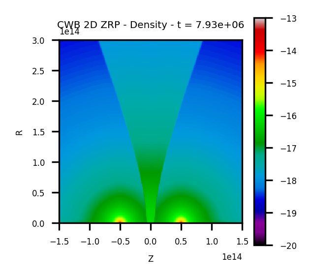
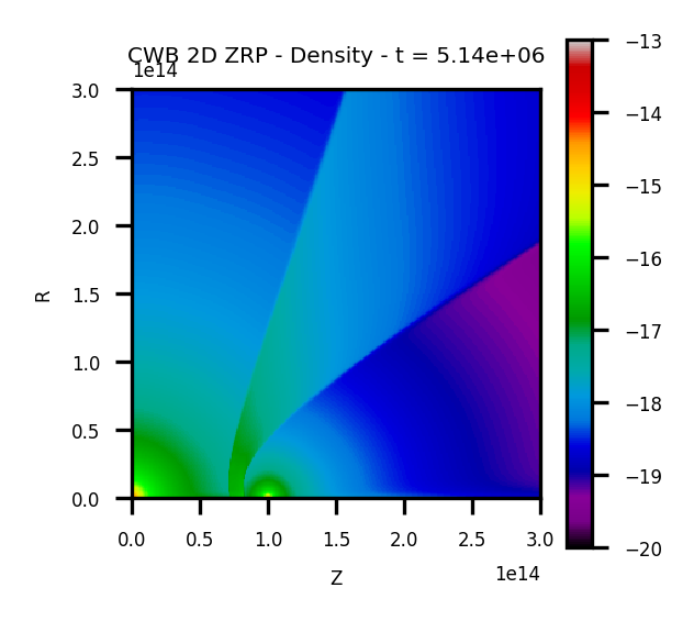
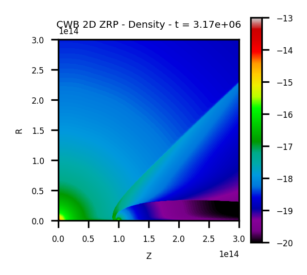
Figure 1: Density distributions in the winds and WCR for 3 different values of $\eta$: $\eta=1.0$ (left), $\eta=0.1$ (middle), $\eta=0.01$ (right). The primary wind parameters and $v_{2}$ were kept fixed, while $\dot{M}_{2}$ was varied. Larger grids than shown were used to calculate the X-ray emission when $\eta<1$. Distances are in cm, and densities in ${\rm g\,cm^{-3}}$.

3 Results

3.1 Opening angles and wind fractions

Prior to studying the X-ray emission from our simulations we first examine how the opening angles of the shocks and CD vary with $\eta$. Here the opening angle, $\theta$, is defined as the angle between the secondary star, the stagnation point, and the shock or CD. Table 1 and Fig. 2 highlight our findings.

Table 1: The opening angles of the primary ($\theta_{1}$) and secondary ($\theta_{2}$) shocks, and the contact discontinuity ($\theta_{\rm CD}$), as a function of $\eta$. All values have an estimated uncertainty of $\pm 2^{\circ}$, except the opening angle of the CD when $\eta=1.0$ which is by defintion known to be precisely $90^{\circ}$. The entirety of the secondary wind is shocked when $\eta\mathrel{\hbox to0.0pt{\lower 3.0pt\hbox{$\sim$}\hss}\raise 2.0pt\hbox{$<$}}0.01$, so the secondary shock does not have an asymptotic opening angle in such cases.

$\eta$	$\theta_{1}$	$\theta_{\rm CD}$	$\theta_{2}$
1.0	109	90	71
0.5	96	79	60
0.2	83	62	42
0.1	73	51	30
0.05	62	42	21
0.02	50	31	7
0.01	44	22
0.005	37	16
0.002	32	10
0.001	30	5

These values are in good agreement with an earlier determination from hydrodynamical simulations (Pittard & Dougherty, 2006). When $\eta=1$ the winds are of equal strength, and the shocks flare out by $\approx 19^{\circ}$ from the CD. The secondary shock has $\theta_{2}=0.0$ (i.e. the secondary wind is completely shocked) when $\eta$ is just above 0.01 (at $\eta=0.01$ the secondary shock is curving back towards the line of symmetry).

As far as we are aware, there are no other measurements of the shock and CD opening angles from hydrodynamical simulations in the literature. However, there have been numerous attempts to determine analytical expressions for the opening angles of the CD. For instance, Girard & Willson (1987) assumed that the shocks were highly radiative (and thus spatially coincident with the CD), and calculated their position based on momentum conservation. Eichler & Usov (1993) report that Girard & Willson (1987)’s results are well approximated by the function

$$\theta\approx 2.1\left(1-\frac{\eta^{2/5}}{4}\right)\eta^{1/3}.$$ (1)

Canto et al. (1996) also investigated the case of highly radiative shocks, and provided a formula for the opening angle (albeit using a different definition for $\theta$). Changing to the usual definition one finds that their Eq. 28 is equivalent to

$$\theta-\tan\theta=\frac{\pi\eta}{\eta-1}.$$ (2)

More recently, the “characteristic” opening angle of an adiabatic wind-wind collision was considered by Gayley (2009). As a result of the shock heating, an increase momentum flux is generated away from the axis, and leads to a greater opening angle than for the case of a radiative WCR. If there is no mixing across the CD, Gayley (2009) finds that

$$\theta=2\tan^{-1}(\eta^{1/4}).$$ (3)

Fig. 2a) shows the functions in Eqs. 1-3 plotted against our results. We find that the Eichler & Usov (1993) and (Canto et al., 1996) formulae are almost identical, while the Gayley (2009) formula produces larger opening angles for $\eta<1$. We also find that modifying Gayley’s formula to $\theta=2\tan^{-1}(\eta^{1/3})$ brings it back into agreement with the other formulae. This is also consistent with the discusion in Sec. 4.1 in Gayley (2009). We further note that while the Eichler & Usov (1993), Canto et al. (1996) and our “modified” Gayley formulae fit the results from our hydrodynamical simulations very well for $0.01\mathrel{\hbox to0.0pt{\lower 3.0pt\hbox{$\sim$}\hss}\raise 2.0pt\hbox{$<$}}\eta\mathrel{\hbox to0.0pt{\lower 3.0pt\hbox{$\sim$}\hss}\raise 2.0pt\hbox{$<$}}1$, the opening angle becomes increasingly divergent at smaller values of $\eta$.

In contrast to the many functions which exist for $\theta_{\rm CD}$, there are no formulae for the opening angles of the shocks, $\theta_{1}$ and $\theta_{2}$, when the WCR is not highly radiative. As a matter of interest we note that multiplying Eq. 3 by a factor of $\approx 1.2$ yields a reasonable fit to $\theta_{1}$, but the opening angle is underestimated when $\eta\mathrel{\hbox to0.0pt{\lower 3.0pt\hbox{$\sim$}\hss}\raise 2.0pt\hbox{$<$}}0.005$. Nevertheless, this shows that Gayley (2009)’s “characteristic” opening angle perhaps better describes $\theta_{1}$ than $\theta_{\rm CD}$. We also notice that the primary shock maintains a roughly constant angle from the CD as a function of $\eta$. Fig. 2b) shows a fit to the primary shock position, assuming that $\theta_{1}=2\tan^{-1}(\eta^{1/3})+\delta\theta$. The best fit has $\delta\theta\approx\pi/9$. Our hydrodynamical simulations do not extend to $\eta<10^{-3}$, so we cannot test whether the primary shock will always achieve an opening angle of at least $20^{\circ}$, as is implied by this function.

Considering now the opening angle of the secondary shock we find that it is reasonably well fit by the function $\theta_{2}=0.658\log_{10}(71.7\eta)$, which implies that the entire secondary wind is shocked when $\eta<1/71.7\approx 0.014$ (Fig. 2c).

Using our approximations for $\theta_{1}$ and $\theta_{2}$, we can determine the fraction of each wind which is shocked as a function of $\eta$. For the primary shock this is $f_{1}=\Omega_{1}/(4\pi)$, where $\Omega_{1}=2\pi(1-\cos\theta_{1})$. For the secondary wind, this fraction is $f_{2}=\Omega_{2}/(4\pi)$, where $\Omega_{2}=2\pi(1+\cos\theta_{2})$. The resulting fractions are shown in Fig. 2d).

There appear to be two cases in the literature where the opening angles are incorrectly calculated. Zabalza et al. (2011) estimated that for small values of $\eta$, $\theta_{\rm CD}\approx\pi\eta$ and $f_{\rm CD}\approx\theta_{\rm CD}^{2}/4\approx(\pi\eta)^{2}/4$. However, for small values of $\eta$, the Canto et al. (1996) analysis actually gives $\theta_{\rm CD}^{3}\approx 3\pi\eta/(1-\eta)\approx 3\pi\eta$ (cf. Sec. 4.1 in Gayley, 2009), which yields $f_{\rm CD}\approx(3\pi\eta)^{2/3}/4$, rather than the expression given by Zabalza et al. (2011). In any case, Fig. 2a) shows that the Canto et al. (1996) analysis overestimates $\theta_{\rm CD}$ at low values of $\eta$. The second occurence is in Lomax et al. (2015), where it is noted in Sec. 4.3 that Canto et al. (1996)’s formula gives an opening angle of $68^{\circ}$ for $\eta=0.058$. In fact, it gives $\theta=43.7^{\circ}$, in agreement with the other formulations in their section.

3.2 The X-ray luminosity and spectral shape

Fig. 3a) shows how the X-ray luminosity calculated from our hydrodynamical simulations scales with $\eta$. It is immediately clear that the proposed scaling by Stevens et al. (1992) is not a good match to the actual variation in $L_{\rm x}$. The scaling suggested by Stevens et al. (1992) goes approximately as $L_{\rm x}\propto\eta^{3/2}$ (at small values of $\eta$), whereas the numerical simulations instead scale approximately as $L_{\rm x}\propto\eta$. Since the distance between the stagnation point and the secondary star, $r_{\rm OB}=\sqrt{\eta}D_{\rm sep}/(1+\sqrt{\eta})$, scales as $\sqrt{\eta}$ for small $\eta$, this implies that $L_{\rm x}\propto r_{\rm OB}^{2}$ when $\eta$ is small, which is akin to the X-ray luminosity scaling in proportion to a “target area” rather than a “characteristic” volume.

Fig. 3a) shows that the exact variation of $L_{\rm x}$ with $\eta$ also depends on the X-ray band concerned, with the variation being slightly stronger in harder bands. This is a result of the shape of the spectrum also being dependent on $\eta$, as shown in Fig. 3b). Previous work claimed that the spectral shape was insensitive to the value of $\eta$ (Pittard & Corcoran, 2002), at least over the range $1.26-10$ keV. However, by examining the spectrum over a greater energy range we now see that there is indeed a small effect. In particular, we see a change in the slope of the continuum, and changes to the strength of the line emission, especially for lines below 1 keV. That the spectrum softens with decreasing $\eta$ is likely caused by the increasing dominance of the shocked primary wind to the X-ray emission, and the increasing obliquity of the primary wind shock, with decreasing $\eta$. We find this to be the case for simulations with other wind speeds too (e.g., both winds blowing at $1500\,\hbox{${\rm{\rm\thinspace km}{\rm\thinspace s}^{-1}\,}$}$ or $3000\,\hbox{${\rm{\rm\thinspace km}{\rm\thinspace s}^{-1}\,}$}$).

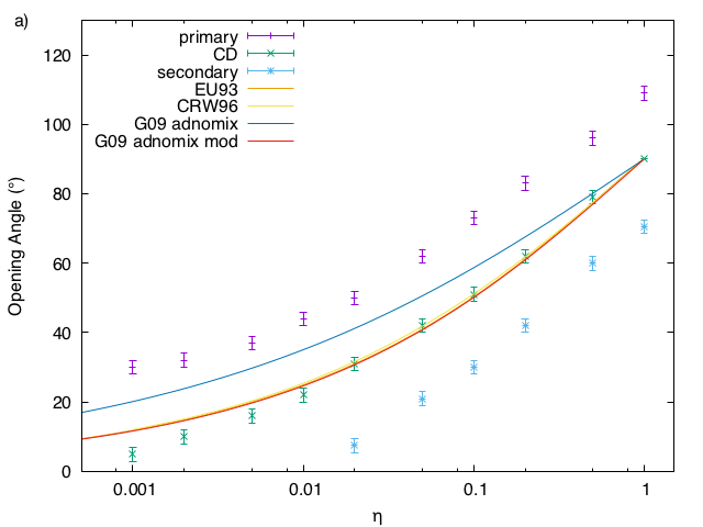
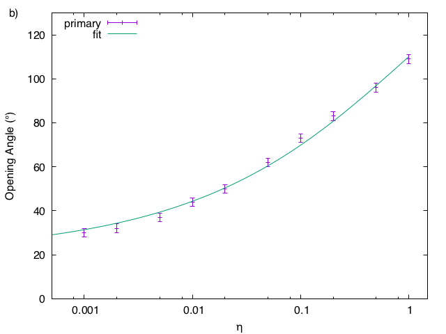
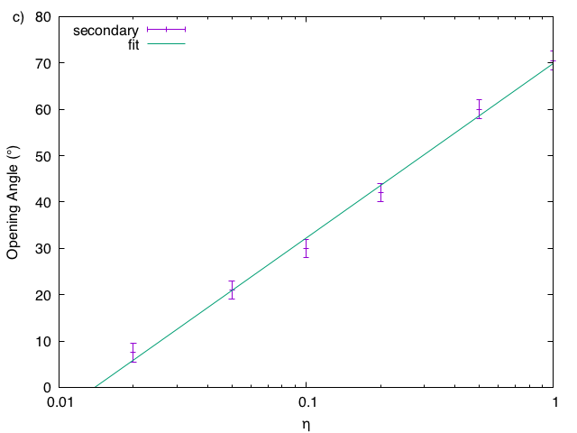
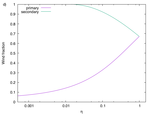
Figure 2: a) Opening angles of the primary and secondary shocks, and the CD. b) Opening angle of the primary shock. c) Opening angle of the secondary shock. d) Fraction of wind shocked.

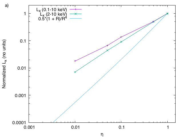
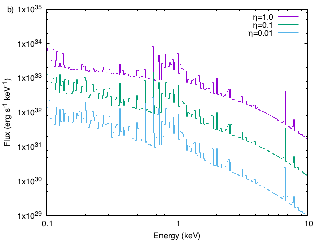
Figure 3: a) Scaling of the X-ray luminosity with $\eta$. Also compared is the scaling suggested by Stevens et al. (1992). b) Variation of the X-ray spectrum with $\eta$. All calculations were based on our standard model parameters, with $\dot{M}_{2}$ varying.

4 Conclusions

We have investigated the structure of and X-ray emission from the colliding stellar winds in massive star binaries. We find that the opening angle of the CD is in good agreement with previous studies for $\eta\mathrel{\hbox to0.0pt{\lower 3.0pt\hbox{$\sim$}\hss}\raise 2.0pt\hbox{$>$}}0.01$, but that these studies overestimate it when $\eta\mathrel{\hbox to0.0pt{\lower 3.0pt\hbox{$\sim$}\hss}\raise 2.0pt\hbox{$<$}}0.01$. We also find that the shocks in the primary and secondary winds flare by about $20^{\circ}$ relative to the CD, and that this is approximately independent of $\eta$. This implies that the opening angle of the primary shock does not tend to zero in the limit $\eta\rightarrow 0.0$. We also find that the X-ray luminosity scales roughly as $L_{\rm x}\propto\eta$, which is not as steep a dependence on $\eta$ as previously conjectured, and that the X-ray spectrum softens slightly as $\eta$ decreases.

It would be very interesting to compare our new predicted scaling ($L_{\rm x}\propto\eta$) with observations. A direct comparison would require observations of systems where one (or both) winds has changed in strength. Such systems do exist. For example, the most massive and luminous binary system in the Small Magellanic Cloud, HD 5980, contains a star which underwent an eruptive event in 1994 (Barbá et al., 1995), during which its mass-loss rate increased while its terminal wind speed decreased. The star has now evolved back towards something like its pre-eruption state (e.g., Foellmi et al., 2008; Georgiev et al., 2011). Earlier X-ray observations revealed orbital phase-dependent variability, but very recently longer-term changes to the X-ray emission, believed to be due to the changes in wind properties of the eruptive component, have been reported (Nazé et al., 2018). Thus HD 5980 would seem to be the perfect system against which to test our new predictions. Unfortunately, the WCR in HD 5980 is expected to be strongly radiative, even when the stars are at apastron, whereas our theoretical predictions are for systems where the WCR behaves largely adiabatically. In future one may hope to find a system similar to HD 5980, but where the WCR behaves adiabatically.

An alternative approach would be to make an indirect comparison to observations, whereby the observed X-ray luminosity from many systems is examined. The most straightforward comparison would involve finding systems where only one of the key parameters changes between them (e.g., the mass-loss rate of the secondary star), while all others are comparable (e.g., the wind speeds and stellar separations remain similar). This task is likely to be difficult, since it will require accurate measurements of these parameters. Relaxing these requirements would yield more potential systems, which would perhaps allow a more indirect, statistical study.

Our simulations were axisymmetric, and ignored details such as the radiative driving of the winds, orbital motion, radiative cooling of the shocked gas, and effects such as non-equilibrium ionization, non-equilibration of electron and ion temperatures, and particle acceleration, all of which will affect either the shock positions and structure of the WCR or the resulting X-ray emission. Some or all of these complications may need to be considered when specific systems are modelled. However, we hope that our results will be a useful guide to the analysis and interpretation of systems with colliding winds.

References

- Anders & Grevesse (1989) Anders E., Grevesee N., 1989, GeCoA, 53, 197
- Barbá et al. (1995) Barbá R. H., Niemela V. S., Baume G., Vazquez R. A., 1995, ApJ, 446, L23
- Canto et al. (1996) Canto J., Raga A. C., Wilkin F. P., 1996, ApJ, 469, 729
- Cazorla et al. (2014) Cazorla C., Nazé Y., Rauw G., 2014, A&A, 561, A92
- Corcoran (2005) Corcoran M. F., 2005, AJ, 129, 2018
- Corcoran et al. (2001) Corcoran M. F., et al., 2001, ApJ, 562, 1031
- Corcoran et al. (2010) Corcoran M. F., et al., 2010, ApJ, 725, 1528
- Corcoran et al. (2017) Corcoran M. F., et al., 2017, ApJ, 838, 45
- De Becker et al. (2006) De Becker M., et al., 2006, MNRAS, 371, 1280
- De Becker et al. (2011) De Becker M., Pittard J. M., Williams P. M., 2011, Société Royale des Sciences de Liège, Bulletin, vol. 80, p. 653-657 (Proceedings of the 39th Liège Astrophysical Colloquium, held in Liège 12-16 July 2010, edited by G. Rauw, M. De Becker, Y. Nazé, J.-M. Vreux, P. Williams)
- Eichler & Usov (1993) Eichler D., Usov V., 1993, ApJ, 402, 271
- Falceta-Gonçalves & Abraham (2012) Falceta-Gonçalves D., Abraham Z., 2012, MNRAS, 423, 1562
- Falle (1991) Falle S. A. E. G., 1991, MNRAS, 250, 581
- Foellmi et al. (2008) Foellmi C., et al., 2008, RMxAA, 44, 3
- Gagné et al. (2012) Gagné M., Fehon G., Savoy M. R., Cartagena C. A., Cohen D. H., Owocki S. P., 2012, in Proceedings of a Scientific Meeting in Honor of Anthony F. J. Moffat held at Auberge du Lac Taureau, St-Michel-Des-Saints, Québec, Canada, held 11-15 July 2011. ASP Conference Series, Vol. 465. San Francisco: Astronomical Society of the Pacific, 2012., p.301
- Gayley (2009) Gayley K. G., 2009, ApJ, 703, 89
- Georgiev et al. (2011) Georgiev L., Koenigsberger G., Hillier D. J., Morrell N., Barbá R., Gamen R., 2011, AJ, 142, 191
- Girard & Willson (1987) Girard T., Willson L.A., 1987, A&A, 183, 247
- Gosset & Nazé (2016) Gosset E., Nazé Y., 2016, A&A, 590, A113
- Gosset et al. (2009) Gosset E., Nazé Y., Sana H., Gregor R., Vreux J.-M., 2009, A&A, 508, 805
- Hamaguchi et al. (2007) Hamaguchi K., et al., 2007, ApJ, 663, 522
- Hamaguchi et al. (2014a) Hamaguchi K., et al., 2014a, ApJ, 784, 125
- Hamaguchi et al. (2014b) Hamaguchi K., et al., 2014b, ApJ, 795, 119
- Hamaguchi et al. (2016) Hamaguchi K., et al., 2016, ApJ, 817, 23
- Henley et al. (2008) Henley D. B., Corcoran M. F., Pittard J. M., Stevens I. R., Hamaguchi K., Gull T. R., 2008, ApJ, 680, 705
- Henley et al. (2005) Henley D. B., Stevens I. R., Pittard J. M., 2005, MNRAS, 356, 1308
- Kee et al. (2014) Kee N. D., Owocki S., ud-Doula A., 2014, MNRAS, 438, 3557
- Kissmann et al. (2016) Kissmann R., Reitberger K., Reimer O., Reimer A., Grimaldo E., 2016, ApJ, 831, 121
- Lamberts et al. (2011) Lamberts A., Fromang S., Dubus G., 2011, MNRAS, 418, 2618
- Lemaster et al. (2007) Lemaster M. N., Stone J. M., Gardiner T. A., 2007, ApJ, 662, 582
- Lomax et al. (2015) Lomax J. R., et al., 2015, A&A, 573, A43
- Luo et al. (1990) Luo D., McCray R., Mac Low M.-M., 1990, ApJ, 362, 267
- Madura et al. (2013) Madura T. I., et al., 2013, MNRAS, 436, 3820
- Mewe et al. (1995) Mewe R., Kaastra J. S., Liedahl D. A., 1995, Legacy, 6, 16
- Myasnikov & Zhekov (1993) Myasnikov, A. V., Zhekov, S. A. 1993, MNRAS, 260, 221
- Nazé et al. (2018) Nazé Y., Koenigsberger G., Pittard J. M., Parkin E. R., Gregor R., Corcoran M. F., Hillier D. J., 2018, ApJ, 853, 164
- Nazé et al. (2012) Nazé Y., et al., 2012, A&A, 546, 37
- Owocki & Gayley (1995) Owocki S. P., Gayley K. G., 1995, ApJ, 454, L145
- Pandey et al. (2014) Pandey J. C., Pandey S. B., Karmakar S., 2014, ApJ, 788, 84
- Parkin & Gosset (2011) Parkin E. R., Gosset E., 2011a, A&A, 530, A119
- Parkin et al. (2011) Parkin E. R., Pittard J. M., Corcoran M. F., Hamaguchi K., 2011b, ApJ, 726, 105
- Parkin et al. (2014) Parkin E. R., Pittard J. M., Nazé Y., Blomme R., 2014, A&A, 570, A10
- Pittard (2007) Pittard J. M., 2007, ApJ, 660, L141
- Pittard (2009) Pittard J. M., 2009, MNRAS, 396, 1743
- Pittard (2017) Pittard J. M., 2018, MNRAS, in preparation
- Pittard & Corcoran (2002) Pittard J. M., Corcoran M. F., 2002, A&A, 383, 636
- Pittard & Dougherty (2006) Pittard J. M., Dougherty S. M., 2006, MNRAS, 372, 801
- Pittard & Stevens (1997) Pittard J. M., Stevens I. R., 1997, MNRAS, 292, 298
- Pittard & Stevens (2002) Pittard J. M., Stevens I. R., 2002, A&A, 388, L20
- Pollock et al. (2005) Pollock A. M. T., Corcoran M. F., Stevens I. R., Williams P. M., 2005, ApJ, 629, 482
- Raassen et al. (2003) Raassen A. J. J., et al., 2003, A&A, 402, 653
- Schild et al. (2004) Schild H., et al., 2004, A&A, 422, 177
- Skinner et al. (2001) Skinner S. L., Güdel M., Schmutz W., Stevens I. R., 2001, ApJ, 558, L113
- Stevens et al. (1992) Stevens I. R., Blondin J. M., Pollock A. M. T., 1992, ApJ, 386, 265
- Sugawara et al. (2015) Sugawara Y., et al., 2015, PASJ, 67, 121
- Usov (1992) Usov V. V., 1992, ApJ, 389, 635
- Williams et al. (2012) Williams P. M., et al., 2012, MNRAS, 420, 2526
- Zabalza et al. (2011) Zabalza V., Bosch-Ramon V., Paredes J. M., 2011, ApJ, 743, 7
- Zhekov et al. (2011) Zhekov S. A., Gagné M., Skinner S. L., 2011, ApJL, 727, L17
- Zhekov et al. (2014) Zhekov S. A., Gagné M., Skinner S. L., 2014, ApJ, 785, 8
- Zhekov & Skinner (2000) Zhekov S. A., Skinner S. L., 2000, ApJ, 538, 808