School of Mechanical Engineering, Xi’an Jiaotong University

School of Mechanical Engineering, Xi’an Jiaotong University

Trailing Waves

Abstract

We report a special phenomenon: trailing waves. They are generated by the propagation of elastic waves in plates at large frequency-thickness ($fd$) product. Unlike lamb waves and bulk waves, trailing waves are a list of non-dispersive pulses with constant time delay between each other. Based on Raleigh-Lamb equation, we give the analytical solution of trailing waves under a simple assumption. The analytical solution explains the formation of not only trailing waves but also bulk waves. It helps us better understand elastic waves in plates. We finally discuss the great potential of trailing waves for nondestructive testing.

Bulk waves and Lamb waves are widely used in non-destructive testing for block structures and thin plates respectively(Li et al., 2013; Su et al., 2006; Drinkwater and Wilcox, 2006; Giurgiutiu, 2005; Raghavan and Cesnik, 2007; Wilcox et al., 2007; Kessler et al., 2002). Lamb waves are generated at small $fd$ product while bulk waves are generated at extremely large $fd$ product. However, the transition state between bulk and Lamb waves has rarely been studied. We have observed a special phenomenon during the detection of thick plates and called it trailing waves. Trailing waves are believed to be the transition state between bulk and Lamb waves. As shown in FIG.1a, a 40-mm-thick aluminum plate was excited by an ultrasonic transducer with a toneburst signal with the center frequency of 3 MHz. The received signal (see FIG.1b) is a list of stable longitudinal pulses with constant time delay and travels at the velocity of longitudinal waves.

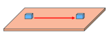
(a)

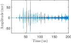
(b)

Figure 1: (a) Experimental setup. Two ultrasonic transducers are placed on the surface of the plate. They are employed as the actuator and receiver respectively. (b) The received trailing waves. The time delay between pulses remains unchanged.

Actually, a similar phenomenon is previously reported and generated by edge excitation(Redwood, 1958, 1959, 1960; Greve et al., 2007, 2008), which is treated as a special case of trailing waves in this paper later.

Consider elastic waves propagating in a free plate, on the upper and lower surface of which the traction force vanishes. Equations of this problem is known as Raleigh-Lamb frequency relations, which can be expressed as follows:

$$\frac{\tan qh}{\tan ph}=-\frac{4k^{2}pq}{(q^{2}-k^{2})^{2}}$$ (1)

$$\frac{\tan qh}{\tan ph}=-\frac{(q^{2}-k^{2})^{2}}{4k^{2}pq}$$ (2)

Where $h$ is half of the thickness $d$. $p$ and $q$ are given by

$$q^{2}=\frac{\omega^{2}}{c_{T}^{2}}-k^{2}$$ (3)

$$p^{2}=\frac{\omega^{2}}{c_{L}^{2}}-k^{2}$$ (4)

Here $c_{T}$ is the velocity of transverse waves, $c_{L}$ is the velocity of longitudinal waves and wavenumber $k$ is equal to $\omega/c_{p}$, where $c_{p}$ is the phase velocity and $\omega$ is the circular frequency. Eqs. (1) and (2) are transcendental equations, which govern the symmetric and antisymmetric modes respectively. These equations can determine the velocities that waves propagate at within plates under a particular $fd$ product. Traditionally, they can be solved only by numerical methods, simple though they are(Rose, 2014). We believe that trailing waves are the solutions of Raleigh-Lamb equation at large $fd$ product. Therefore, we focus on the solutions under large $fd$ product and get the approximate analytical solutions under a simple assumption. Firstly, we consider the symmetric modes. In the dispersion curve, the nearly non-dispersive region where $c_{p}\thickapprox c_{L}$ is considered and the region gets larger by the increasing of $fd$ product. Based on this consideration, the value of $k/\left(\omega/c_{L}\right)$ is very close to unity and Eq. (3) becomes

$$q^{2}=\frac{\omega^{2}}{c_{L}^{2}}(\frac{c_{L}^{2}}{c_{T}^{2}}-1)$$ (5)

Substituting Eq. (5) into Eq. (1), we can write

$$ph\tan ph=-\frac{h}{\varepsilon}\gamma$$ (6)

Where

$$\varepsilon=4\frac{c_{d}}{\omega}\frac{\sqrt{\left(c_{L}/c_{t}\right)^{2}-1}}{\left[\left(c_{L}/c_{t}\right)^{2}-2\right]^{2}}=\frac{c_{L}}{\omega}\frac{\left(1-2\sigma\right)^{\frac{3}{2}}}{\sigma^{2}},\gamma=\tan qh$$ (7)

Here $\sigma$ is Poisson’s ratio. Considering large $fd$ product, we take the assumption that $\frac{h}{\varepsilon}\gamma$ is very large. This assumption will be inaccurate only in a few cases where $\gamma$ is small. This limitation weakens by the increase of $fd$ product ($\frac{h}{\varepsilon}$ gets larger). Let assume that the form of solution is $ph=r+is+\left(n+\frac{1}{2}\right)\pi$ where $r$ and $s$ are small. We get that$\tan\left(ph\right)\thickapprox-\left(r+is\right)^{-1}$, which accords with the right hand side of Eq.6. The term $n\pi$ meets the periodicity of tangent function. Eq. (6) may be written as

$$r+is+\left(n+\frac{1}{2}\right)\pi\thickapprox\frac{h\gamma}{\varepsilon}\left(r+is\right)$$ (8)

Which gives

$$r\thickapprox\frac{\left(n+\frac{1}{2}\right)\pi}{\gamma h/\varepsilon-1}\thickapprox\frac{\varepsilon}{h\gamma}\left(n+\frac{1}{2}\right)\pi s\thickapprox 0$$ , (9)

According to Eq. (4), the phase velocity of symmetric modes is

$$c_{p,s}=\left[\frac{1}{c_{L^{2}}}-\left(n+\frac{1}{2}\right)^{2}\pi^{2}\left(h\omega-\frac{c_{L}}{\gamma}\frac{\left(1-2\sigma\right)^{\frac{3}{2}}}{\sigma^{2}}\right)^{-2}\right]^{-\frac{1}{2}}$$ (10)

where $n$ represents different modes of trailing waves. The group velocity $c_{g}$ can be obtained by the relation $c_{g}=c_{p}^{2}\left(c_{p}-\omega\frac{\mathrm{d}c_{p}}{\mathrm{d}\omega}\right)^{-1}$. The solution of anti-symmetric modes is almost the same as above. Therefore, the phase velocity of anti-symmetric modes is

$$c_{p,a}=\left[\frac{1}{c_{L^{2}}}-n^{2}\pi^{2}\left(h\omega+\gamma c_{L}\frac{\left(1-2\sigma\right)^{\frac{3}{2}}}{\sigma^{2}}\right)^{-2}\right]^{-\frac{1}{2}}$$ (11)

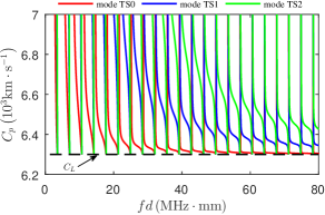
(a)

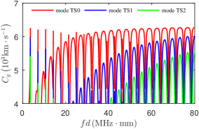
(b)

Figure 2: Dispersion curves of trailing waves (symmetric modes). (a) The phase velocity. (b) The group velocity.

FIG. 2a and FIG. 2b show the value of $c_{p}$ and $c_{g}$ of symmetric modes as a function of $fd$ product. The singular value of group velocity is due to numerical instability. At the region where $c_{p}\thickapprox c_{L}$, the group velocity arrives its local maximum. While at the region where the phase velocity changes rapidly, the group velocity approaches zero and the corresponding frequencies are called the cut-off frequencies $f_{c}$. Note that the definition of trailing wave modes is quite different from the Lamb wave modes. Classical Lamb wave modes are separated by $f_{c}$ while trailing wave modes are determined by variable $n$ in Eqs. (10) and (11). Each trailing wave mode consists of a cluster of adjacent Lamb wave modes. These differences are then demonstrated by an experiment. In our experiment, the symmetric modes of trailing waves were obtained by edge excitation (FIG. 3). Geometric symmetry excitation could eliminate the antisymmetric modes. This means the similar phenomenon previously reported as secondary signals etc. is actually the symmetric modes of trailing waves. In the time-frequency spectrogram (3c), the experimental trailing waves are consistent with the theoretical result (TS0 mode) while higher modes are obscure.

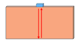
(a)

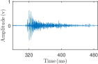
(b)

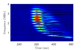
(c)

Figure 3: (a) Experimental setup. One ultrasonic transducer is employed as the Self-Transmitting and Self-Receiving sensor. The sensor is excited by a broadband toneburst signal with the frequency from 25 KHz to 4 MHz. (b) The received trailing waves of symmetric modes. (b) The time-frequency spectrogram of the experimental signal, compared with TS0 mode (black line).

Next, the formation of trailing waves will be discussed based on the analytical solution. We will mainly analyze the symmetric modes. As expressed in Eq. (10), the modulation factor $h\omega$ (MAF) and the periodic factor $\gamma$ (PAF) play key roles in the formation of trailing waves. Expanding Eq. (7), we get

$$\gamma=\tan qh=\tan\left(2\pi fh\sqrt{\frac{1}{c_{T}^{2}}-\frac{1}{c_{p}^{2}}}\right)$$ (12)

with the period of $\triangle f=1/\left(2h\sqrt{\frac{1}{c_{T}^{2}}-\frac{1}{c_{p}^{2}}}\right)$. PAF forces the phase and group velocity repeating in the period of $\triangle f$ in frequency domain. According to Fourier transform, the periodicity in frequency domain leads to uniformly-spaced sampling in time domain, which means the waves will split into a list of waves with constant time delay. The time delay, determined by PAF, is $\Delta t=1/\Delta f$. Additionally, the cut-off frequency $f_{c}$ is $f_{c}=n/\left(2h\sqrt{\frac{1}{c_{T}^{2}}-\frac{1}{c_{p}^{2}}}\right)$. The group velocity approaches 0 near $f_{c}$ because the phase velocity goes infinite. On the other hand, the amplitude distribution of trailing waves is mainly determined by MAF. As the $fd$ ($h\omega$) product goes larger, the region where $c_{p}\thickapprox c_{L}$ becomes larger, which makes the result more accurate; meanwhile, a larger range of group velocity becomes closer to $c_{L}$. The problem of amplitude distribution can be regarded as a reverse process of Fourier transform of periodic signal that repeats in the time domain. We simplified the group velocity dispersion curve of trailing waves into periodic rectangular pulses $F\left(\omega\right)$ that repeat in the frequency domain. The period of $F\left(\omega\right)$ is determined by $\triangle f$ : $\omega_{T}=2\pi\triangle f$. The duty cycle ($\omega_{t}/\omega_{T}$) is qualitatively described by and positively associated with the region where $c_{g}$ is close to $c_{L}$. The amplitude distribution of trailing waves can be obtained by inverse Fourier transform of $F\left(\omega\right)$:

$$f_{n} =\frac{1}{\omega_{T}}\int_{-\frac{\omega_{T}}{2}}^{\frac{\omega_{T}}{2}}F\left(\omega\right)e^{jn\omega t_{0}}d\omega$$

$$=\frac{\omega_{t}}{\omega_{T}}{\rm Sa}\left(\frac{nt_{0}\omega_{t}}{2}\right),n=0,\pm 1,\pm 2\ldots$$ (13)

Where $t_{0}=\frac{2\pi}{\omega_{T}}$ and ${\rm Sa}$ is sampling function. It is noted that although the negative part of time delay $nt_{0}$ has no physical meaning, the actual amplitude distribution of the pulses in the trailing waves equals to the sum of both negative and positive part, which is

$$f\left(n\right)=\begin{cases}f_{n}&n=0\\ f_{n}+f_{-n}&n=1,2,3\ldots\end{cases}$$ (14)

Actually, Eq. (14) can not quantitatively described the amplitude distribution since the duty cycle is a qualitative description variable for $c_{g}$. However, qualitative equation still has the ability to analyze the amplitude distribution of trailing waves. From Eq. (14), it can be seen that the amplitude of first pulse increases with the duty cycle. As shown in FIG. 4, the first pulse contains the most energy of trailing waves when duty cycle approaches one, which happens at large $fd$ product.

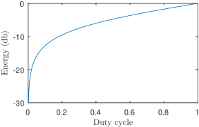
Figure 4: The energy of first pulse.

Under this condition, the secondary pulses of trailing waves vanish and the trailing waves are simplified to longitudinal bulk waves. This indicates that Lamb waves, trailing waves and bulk waves are three kind of waves in traction-free plates that governed by Raleigh-Lamb equation.

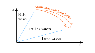
Figure 5: Forming conditions of bulk waves, trailing waves and Lamb waves. The interaction with boundaries will be enhanced by the increasing of $\lambda/d$.

The major formative factor of these three kind of waves is the ratio of wavelength to thickness ($\lambda/d$), which determines how waves interact with boundaries (FIG.5). The incident waves in infinite media, where boundaries have no influence on wave propagation, generate bulk waves. Trailing waves are generated when incident waves interact several times with boundaries. The waves reflecting and refracting with boundaries for infinite times generate Lamb waves.

Besides Lamb waves and bulk waves, trailing waves provide a completely new way for ultrasonic-based damage detection, with unique advantages for thick plates. Generally, the detection of thick plates can be completed by surface scan of bulk waves. High resolution can be achieved by bulk waves, but the detection efficiency will be low because only a small area can be detected by single excitation. On the other hand, there will be limitations if choosing Lamb waves. Although the detection by Lamb waves can be completed rapidly, it brings great difficulties under large $fd$ product. High frequency results in high resolution while more complex and more modes will be generated; low frequency leads to much worse resolution than bulk waves. With high excitation frequency and guided-wave-like propagation mode, trailing waves are able to achieve high resolution and high detection efficiency at the same time. Meanwhile, the disadvantage of trailing-waves-based damage detection is: a pulse train of reflection rather than a single pulse will complicate the interpretation of signals.

In summary, we obtain the analytical solution of trailing waves by Raleigh-Lamb equation at large $fd$ product. Based on PAF and MAF, we explain the formation of trailing waves and bulk waves. Compared with the symmetric modes of trailing waves that generated in the experiment, our result is validated. Based on the analysis, we find that not only Lamb waves but also trailing waves and bulk waves are governed by Raleigh-Lamb equation. Trailing waves also have great potential on resolution and detection efficiency for damage detection of thick plates.

References

- Li et al. (2013) C. Li, D. Pain, P. D. Wilcox, and B. W. Drinkwater, Ndt I& E International 53, 8 (2013).
- Su et al. (2006) Z. Q. Su, L. Ye, and Y. Lu, Journal of Sound and Vibration 295, 753 (2006).
- Drinkwater and Wilcox (2006) B. W. Drinkwater and P. D. Wilcox, Ndt I& E International 39, 525 (2006).
- Giurgiutiu (2005) V. Giurgiutiu, Journal of Intelligent Material Systems I& Structures 16, 291 (2005).
- Raghavan and Cesnik (2007) A. C. Raghavan and C. E. S. Cesnik, Shock I& Vibration Digest 39, 91 (2007).
- Wilcox et al. (2007) P. D. Wilcox, G. Konstantinidis, A. J. Croxford, and B. W. Drinkwater, Proceedings Mathematical Physical I& Engineering Sciences 463, 2961 (2007).
- Kessler et al. (2002) S. S. Kessler, S. M. Spearing, and C. Soutis, Smart Materials I& Structures 11, 269 (2002).
- Redwood (1958) M. Redwood, Proceedings of the Physical Society of London 72, 841 (1958).
- Redwood (1959) M. Redwood, Journal of the Acoustical Society of America 31, 442 (1959).
- Redwood (1960) M. Redwood, Mechanical waveguides : the propagation of acoustic and ultrasonic waves in fluids and solids with boundaries (Pergamon Press, 1960).
- Greve et al. (2007) D. W. Greve, P. Zheng, and I. J. Oppenheim, 2007 Ieee Ultrasonics Symposium Proceedings, Vols 1-6 , 1120 (2007).
- Greve et al. (2008) D. W. Greve, P. Zheng, and I. J. Oppenheim, Smart Materials I& Structures 17 (2008), Artn 035029 10.1088/0964-1726/17/3/035029.
- Rose (2014) J. L. Rose, Ultrasonic guided waves in solid media (Cambridge University Press, 2014).