Radio interferometric observation of an asteroid occultation

Abstract

The occultation of the radio galaxy 0141+268 by the asteroid (372) Palma on 2017 May 15 was observed using six antennas of the Very Long Baseline Array (VLBA). The shadow of Palma crossed the VLBA station at Brewster, Washington. Owing to the wavelength used, and the size and the distance of the asteroid, a diffraction pattern in the Fraunhofer regime was observed. The measurement retrieves both the amplitude and the phase of the diffracted electromagnetic wave. This is the first astronomical measurement of the phase shift caused by diffraction. The maximum phase shift is sensitive to the effective diameter of the asteroid. The bright spot at the shadow’s center, the so called Arago–Poisson spot, is clearly detected in the amplitude time-series, and its strength is a good indicator of the closest angular distance between the center of the asteroid and the radio source. A sample of random shapes constructed using a Markov chain Monte Carlo algorithm suggests that the silhouette of Palma deviates from a perfect circle by $26\pm 13\%$. The best-fitting random shapes resemble each other, and we suggest their average approximates the shape of the silhouette at the time of the occultation. The effective diameter obtained for Palma, $192.1\pm 4.8$ km, is in excellent agreement with recent estimates from thermal modeling of mid-infrared photometry. Finally, our computations show that because of the high positional accuracy, a single radio interferometric occultation measurement can reduce the long-term ephemeris uncertainty by an order of magnitude.

1 Introduction

Observations of lunar occultations provided the first accurate positions for compact extragalactic radio sources, and contributed to the discovery of quasars (Hazard et al. 1963; Oke 1963; Schmidt 1963). Lunar occultations have also been used to derive high-resolution images of radio sources from the Fresnel diffraction fringes observed with single-dish telescopes (e.g., Hazard et al. 1967; Maloney & Gottesman 1979; Schloerb & Scoville 1980; Cernicharo et al. 1994). Restoring techniques developed by Scheuer (1962) and von Hoerner (1964) were utilized in these works. More recently, the brightness distributions of compact radio sources have mainly been studied using interferometric arrays such as Very Long Baseline Interferometry (VLBI). Nevertherless, radio occultations by solar system bodies remain useful for determining the properties of the foreground objects, including planetary atmospheres and coronal mass ejections from the Sun (Kooi et al. 2017; Withers & Vogt 2017). The basic principles and methods of radio (lunar) occultation measurements were described by Hazard (1976).

One application of radio occultations is the possibility of determining the size of an asteroid by a single, short measurement. This measurement also gives an accurate position of the asteroid at the time of the occultation, and can be used to constrain its shape, particularly when the angular size of the object is too small to be imaged with any currently available instruments. The radio occultation method for asteroids was first demonstrated by Lehtinen et al. (2016) who used the 100m Effelsberg telescope to observe the occultation of a radio galaxy by the asteroid (115) Thyra. As discussed by Lehtinen et al. (2016), at radio wavelengths the shadow of the asteroid is often dominated by diffraction fringes. The observed diffraction pattern depends on the wavelength, and the size and the distance of the asteroid. A rule of thumb is that a sharp shadow is observed when the Fresnel number, $F$, is greater than 1, whereas a diffraction pattern in the Fraunhofer regime is observed for $F\leq 1$ (e.g., Trahan & Hyland 2014). In the latter case the diffraction pattern is much larger than the geometrical shadow. The Fresnel number is defined by $F=a^{2}/(d\lambda)$, where $a$ and $d$ are the radius and the distance of the occluder, and $\lambda$ is the wavelength.

The astrophysical interest in asteroid size determination lies, for example, in the fact that it is needed for estimating the bulk density, which in turn contains information of the composition and internal structure of an asteroid (Carry, 2012). So far, only a third of the density estimates are more precise than 20% (Carry, 2012). Increasing the sample of asteroids with accurate density estimates is important given the large variation in asteroid diameters (and hence in self-gravity), as well as the potentially large variation in interior structure, which reflects the collisional history of the solar system. Another challenge is the determination of the mass, which for an isolated asteroid, is based on orbital deflections during close encounters with other asteroids. In the fortuitous situation in which an asteroid has a satellite, its orbit around the primary body can be used to substantially constrain the mass. Radio occultation observations can help to discover binary systems by virtue of diffraction fringes from the satellite.

Here, we report on an asteroid occultation observation using the Very Long Baseline Array (VLBA; Napier et al. 1994), operated by the Long Baseline Observatory. During an occultation, the direct path to the source blocked and diffracted electromagnetic radiation arrives at the receiver. The ampltitude and phase of the diffracted wave are different from those measured for the unobstructed wave. In contrast to most optical interferometry, in which the correlated signal power is detected (for example, in a CCD), radio interferometers correlate the voltages from pairs of telescopes, and are able to measure the phase as well as amplitude of the correlated signals. In the course of calibration and imaging, one can correct for both phase and amplitude variations and recover the complex effects of the occultation. This offers important advantages over single-dish measurements, as two quantities characterizing the diffracted wavefront are measured simultaneously, and, as shown in this paper, the phase is more sensitive to the asteroid size than the amplitude. The occultation observation of Lehtinen et al. (2016) with a single total power receiver had problems with reconciling the expected diffraction pattern from a contiguous occluder of the size of Thyra. In particular, the brightness of the first diffraction maxima could not be explained. In the present work, the measured amplitude and phase curves can be satisfactorily explained in terms of the Fresnel-Kirchoff diffraction theory, and lead to a plausible model for the asteroid silhouette.

The background source in the present observations is the active galactic nucleus (AGN) 0141+268 (J0144+270), associated with a BL Lac type galaxy (Lister et al., 2016). At the wavelength used ($\lambda=4.2$ cm), the source consists of a compact nucleus, $<3$ milliarcseconds (mas), and a faint jet. An image of the source at 8.7 GHz from the VLBA experiment VCS-II-D/BG219D (2014 June 9; Gordon et al. 2016), is shown in Figure 1..

The occluder is the asteroid (372) Palma, which resides in the outer parts of the main asteroid belt (semimajor axis $a=3.15$ au, eccentricity $e=0.26$, inclination $i=23\fdg 8$). The SMASSII spectroscopic classification of Palma is B (Bus & Binzel, 2002), geometric albedo $p_{\rm V}=0.059\pm 0.009$ (Masiero et al., 2012), and bulk density $1.40\pm 0.18$ g cm^-3 (Carry, 2012). Palma is not associated with any of the currently known asteroid families. Recent estimates for its diameter from thermal modeling of mid-infrared photometric data range from 187 to 191 km (Carry 2012; Masiero et al. 2014).

The paper is organized as follows. In Section 2, we present the prediction for the occultation observable with one of the VLBA antennas, located in Brewster, Washington, USA. In Section 3 we describe the VLBA observations. In Section 4, the observed visibilities are interpreted in terms of the Fresnel-Kirchhoff diffraction theory applied to different silhouette models. The results are discussed in Section 5.

Figure 1: Image of the active galactic nucleus 0141+268 (J0144+270) at 8.7 GHz from the VLBA survey VCS-II (Gordon et al., 2016). The synthesized beam size of the observation is shown in the bottom right ($2.2\times 1.3$ mas, P.A. $17\fdg 4$). The predicted closest position of (372) Palma as seen from Brewster is indicated with a plus sign (outside the frame). The white arc marks the approximate silhouette of the asteroid, assuming that it is a circular disk with a diameter of 190 km (76 mas).

Figure 2: Shadow path of (372) Palma on 2017 May 15, near Brewster, Washington. The arrow shows the distance the shadow traveled in 10 seconds (510 km). The projections of the geometric shadow of the asteroid are shown with small ellipses at intervals of 1 second. The asteroid silhouette is approximated by a circular disk with a radius of 96 km. The two bigger ellipses show the first maxima of the diffracted intensity pattern outside the geometric shadow, $4$ s before and after its closest approach to Brewster. The prediction for the size of the bright rings is based on the 96 km circular disk.

2 Occultation Prediction

Palma was predicted to occult the AGN 0141+268 (J0144+270) on 2017 May 15, as seen from the Brewster VLBA station (br-vlba). The predictions were made using the LinOccult program. LinOccult requires three auxiliary data sets. (1) The position of the background object was adopted from the latest Radio Fundamental Catalog (RFC), available at http://astrogeo.org/rfc (Petrov et al. 2008; Petrov & Kovalev 2017). (2) The orbital elements of the asteroid were taken from a database provided by Lowell Observatory. (3) The ephemerides of the major planets were obtained using the JPL HORIZONS service.

The asteroid radius ($a\sim 96$ km; Carry 2012; Masiero et al. 2014), and its distance at the time of the observation ($d\sim 3.436$ au) imply a Fresnel number of 0.43 at $\lambda=4.2$ cm. This means that a Fraunhofer diffraction pattern was observable on the Earth. The predicted shadow path in the vicinity of Brewster is shown in Figure 2. According to this prediction, the ground speed of the shadow was 51 km s^-1 near Brewster, and the telescope was located just inside the geometric shadow at the time of the closest approach, UT 14:31:23. At this time, the asteroid and the radio galaxy were in the east, at an elevation of $42^{\circ}$. The projection of the shadow on the Earth is therefore elongated in an east-west direction. Also shown in this figure are the projections of the first bright ring of the diffracted intensity pattern, 4 s before and after the deepest occultation. The radius of the bright ring (in a plane perpendicular to the line-of-sight to the source) is $\sim 215$ km, calculated assuming a circular occluder with a radius of 96 km. The detectable diffraction fringes are expected to extend to a distance approximately twice this radius. Taking the projection effect into account, the maximum distance from the shadow center where the diffraction fringes could possibly be detected is $\sim 630$ km. This means that other VLBA antennas than Brewster received unobscured signal from 0141+268.

3 Very Long Baseline Array Observations

The occultation was observed by six VLBA antennas: br-vlba (Brewster), fd-vlba (Fort Davis), kp-vlba (Kitt Peak), la-vlba (Los Alamos), pt-vlba (Pie Town), and ov-vlba (Owens Valley) located in the continental United States. The lengths of baselines to br-vlba ranged from 1.2 to 2.3 thousand kilometers. The central frequency of the observations was 6.996 GHz, and the total bandwidth was 256 MHz. Both right and left circular polarizations were recorded with 2 bits per sample.

The observations started at UT 14:00, on May 15, with a five minute scan on the strong radio source 0149+218, which was used as the fringe finder and bandpass calibrator. Thereafter, the antennas tracked 0141+268 until UT 15:00 with 10 s long pauses every 5 minutes. The occultation was predicted to be deepest at 14:31:23. System temperature ranged from 25 to 35 K, and the system equivalent flux density was in the range 240–290 Jy.

The data were correlated in the Science Operations Center in Socorro, using NRAO’s implementation of the DiFX (Distributed FX) software correlator (Deller et al. 2011; FX means that the Fourier transform is applied before the cross-multiplication of signals). The correlator integration time was 0.25 s and the frequency resolution was 250 kHz. Further processing was done with the ${\cal PIMA}$ VLBI data analysis software package. The data were split into 290 s long segments, and the residual phase delay and group delays were fit into the spectrum of the cross-correlation function produced by the correlator, also known as the fringe visibility. The fringe visibilities were counter-rotated to the contribution of the group delay and the phase delay rate, and coherently averaged over frequency. For details on the fringe fitting procedure, we refer the reader to Petrov et al. (2011) and Thompson et al. (2017).

Only one antenna, br-vlba was affected by the occultation. During the occultation, the power of the signal recorded at br-vlba dropped, and the optical path delay from the source to the antenna changed with respect to the unobscured situation. Even though the $(u,v)$ visibility coordinates for the five baselines are different, and one can expect differences in the amplitudes and, especially, the phases between these, the changes in the normalized amplitudes and the relative phases during the occultation should be similar for all of them. For the purposes of the present study we only need to retrieve these relative changes. Therefore, after the fringe fitting, we computed arithmetic averages over the five baselines. The residual fringe phases were stacked with zero mean, and the stacked fringe amplitudes were normalized to unity. The change in the path delay at br-vlba propagates directly to the visibility phases, $\Phi$, for all the five baselines including Brewster. In contrast, the change in the normalized visibility amplitude, $|V|$, during the occultation is proportional to the square root of the relative power drop measured at br-vlba, that is, $|V|\propto\sqrt{\frac{\Delta P_{\rm B}}{P_{\rm B}}}$. The effects removed in the calibration process occur on long timescales compared with the brief occultation event.

Figure 3: Stacked visibility amplitudes, $<|V|>$ (a), and phases, $<\Phi>$ (c), during the occultation. The vertical bars show the rms scatter of the normalized amplitude (a) and the phase (c) (calculated excluding a 20 s period around the occultation). The averaging is performed over five VLBA baselines including Brewster. The time-series are smoothed to a resolution of 0.35 s. The amplitude of the unobscured signal is normalized to unity. The right panels ((b) and (d)) show 12 s portions of the amplitude and phase time-series in terms of the rms scatter (vertical bars). Time-inverted amplitude and phase curves (green and orange curves) are superposed to highlight asymmetries. The bottom panel (e) shows the amplitude vs. phase diagram. The points before and after the deepest occultation are indicated with blue and red, respectively. The cross shows the rms scatters of the two quantities.

For individual baselines, the rms noise levels over the 290 s interval, including the occultation (excluding 20 s around the closest approach), range from 0.112 to 0.147 for the normalized amplitudes, and from 0.128 to 160 rad for the phases. The rms values of the stacked amplitudes and phases for the same period are 0.079 and 0.083 rad, respectively. In order to reduce the scatter in residual fringe amplitudes and phases, at the expense of the time resolution, we applied a weak Gaussian filter using the kernel $K(t,t_{0})=\exp\left\{-(t-t_{0})^{2}/(2a^{2})\right\}$, where $t$ is time and the parameter has the value $a=0.35$ s.

The stacked fringe phases exhibit fluctuations of $\sim\!0.1$ rad on time scales of 50–100 s due to changes in the atmosphere path delay and possible phase and frequency offsets of the station clocks. In order to alleviate the contribution of these smooth fluctuations, we first fitted the phase pattern during the occultation by the sinc function, and subtracted this model from the time-series. Therafter, a low-pass Gaussian filter with $a=10$ s was applied to the residuals. Finally, the smoothed, low-pass-filtered phases were subtracted from those filtered with $a=0.35$ s. These residual phases and amplitudes are used in the subsequent analysis. The rms scatter of this 270 s long dataset, with $\pm 10$ s around the occultation excluded, is 0.033 for the normalized amplitude and 0.043 rad for the phase.

The stacked and smoothed residual amplitudes and phases are shown in Figure 3 (panels (a) and (c)). A zoomed-in view of the time-series, normalized to the rms scatter, is presented on the right of this figure (panels (b) and (d)). In panel (b), the zero level corresponds to the average normalized amplitude of the unobscured signal. Also shown in panels (b) and (c) are the amplitudes and phases with the time axis reversed. This is to highlight asymmetries between the immersion and emergence sides. The intensity minima caused by the obscuration of the background source, and the Arago–Poisson spot between these minima are detected at levels exceeding $10\,\sigma$ in the amplitude curve. The maximum phase shift associated with the deepest occultation is 1.3 radians ($\sim 30\,\sigma$). The amplitude maxima on both sides of the deep minima, corresponding to the first intensity maxima of the diffraction pattern, are detected at levels of 3 $\sigma$ (immersion) and 5 $\sigma$ (emergence). The depths of the phase minima occurring at the same time, are approximately 8 $\sigma$ (immersion) and 6 $\sigma$ (emergence). The shapes of the amplitude bumps and the phase dips are different on the immersion and emergence sides, the difference being more prominent in the phase curve. The difference is also visible in the amplitude versus phase plot shown in panel e of Figure 3. In this diagram, the center of the occultation curve, with the maximum phase shift lies on the right, and the unobscured baselines before and after the occultation correspond to the concentration of points around phase 0, amplitude 1. The visibilities on the immersion and emergence sides of the occultation are plotted with blue and red symbols, respectively.

Figure 4: Top row: opaque circular disk (a) and the intensity (b) and phase (c) patterns of a plane wave diffracted by this obstacle. The radius of the occluder and its shortest projected distance from the background source (plus sign) are adjusted to agree with the occultation curves produced by Palma. The silhouette is drawn on the celestial sphere, whereas the diffraction patterns are projections onto a plane perpendicular to the direction of the radiation source. The dashed line in panel (a) shows the path of the asteroid in the sky relative to the background source. The dashed lines in panels (b) and (c) indicate the cross section of the diffraction pattern measured at Brewster. Bottom row: visibility amplitude versus phase (d) and the amplitude (e) and phase (f) profiles along the dashed lines shown in the top row. In panel (d), the observing points corresponding to the immersion and the emergence are indicated with blue and red, respectively. In the calculated diagram, these two sides overlap perfectly, because the obstacle is symmetric. The observed time-series of the visibility amplitudes and phases during the occultation of Palma are shown with thick green and orange lines. The time range ($\sim 30$ s) corresponds to the spatial range ($\sim 1200$ km) of the images. The residuals after subtracting the model from the observations are shown in the bottom of panels (e) and (f). The residuals in phase are shifted down by 1.2 radians for clarity (panel (f)). The rms scatters of the normalized amplitude and the phase are indicated with vertical bars in panels (e) and (f), and with a cross in panel (d).

4 Predicted Visibilities from Silhouette Modeling

4.1 Circular Disk

We first model the occultation curves assuming that the occluder is a circular disk. In the case in which the background source is point-like, implying that the incident wavefront is planar, the formulae for the complex diffracted amplitude are given, for example, by Roques et al. (1987) (Eqs. B2 and B4 in their Appendix B) and by Aime et al. (2013) (their Sect. 5.3). The finite size of the background source can give rise to a smoothing effect (Roques et al., 2008), but in the present observations this effect is negligible; 99% of the flux comes within an angular radius of $\sim 3$ mas, which is much smaller than the angular Fresnel scale, $\sqrt{\lambda/2d}\sim 40$ mas. For this estimate we reprocessed the VCS-II/BG219D VLBA segment observed on 2014 June 9 (Gordon et al., 2016), and produced the 8.7 GHz image of 0141+268 shown in Figure 1. To examine the magnitude of this smoothing effect, we calculated the amplitude and phase curves from a circular occluder using the actual radio map, and found no visible difference from the calculation that used a point source.

The three input parameters of the circular disk model are the asteroid radius, $a$, the perpendicular distance, $\Delta$, of the Brewster antenna from the center of the shadow path, and the time, $t_{0}$, of the closest approach. The set of input parameters that could produce the closest match to the observed visibility amplitudes and phases was determined by finding the minimum of a reduced $\chi^{2}$ function. We compare both amplitudes and phases to the model predictions, and define the reduced $\chi^{2}$ function by

$$\begin{array}[]{lcl}\chi^{2}&=&\frac{1}{n-p}\sum_{i=1}^{n}\left(\frac{|V|_{i}^{\rm obs}-|V|_{i}^{\rm calc}}{\sigma_{i}^{|V|}}\right)^{2}\\ &&+\frac{1}{n-p}\sum_{i=1}^{n}\left(\frac{\Phi_{i}^{\rm obs}-\Phi_{i}^{\rm calc}}{\sigma_{i}^{\Phi}}\right)^{2}\;,\end{array}$$ (1)

where $n$ is the number of the data points, $p$ is the number of free parameters (here 3), $|V|_{i}$ is the visibility amplitude, and $\Phi_{i}$ is the visibility phase. The superscripts “obs” and “calc” refer to the observed and calculated values, respectively. For acceptable models, the reduced chi-square, that is, chi-square divided by the degrees of freedom as defined in Eq. 1 should be less than 2.5 (see, e.g., Lampton et al. 1976).

The values of the radius, and the distance and time of the closest approach found by this minimization are $a=95.9\pm 2.4$ km, $\Delta=-31.6\pm 3.4$ km, and $t_{0}=$ UTC 14:31:19.63 $\pm 0.07$ s (Coordinated Universal Time). The solution obtained, with the reduced chi-square $\chi^{2}=3.76$, is not particularly good. The parameters of this and other models tested in the present paper are listed in Table 4.1.

Table 1: Best-fit parameters of silhouette models

Model	$a_{\rm eff}$	$\Delta$	$t_{0}$	Other Parameters	$\chi^{2}$
	(km)	(km)	UTC 14:31 +
circle	$95.9\pm 2.4$	$31.6\pm 3.4$	$19.63\pm 0.07$ s		3.76
polyhedral model 1	$95.8\pm 2.7$	$26.1\pm 3.9$	$19.66\pm 0.07$ s		4.61
polyhedral model 2	$97.2\pm 2.1$	$34.7\pm 2.7$	$19.57\pm 0.07$ s		6.01
model 1 rotated by $180^{\circ}$	$96.3\pm 2.7$	$25.1\pm 3.9$	$19.69\pm 0.07$ s		3.53
ellipse	$96.1\pm 2.4$	$25.4\pm 4.5$	$19.68\pm 0.07$ s	$e=0.40\pm 0.13$, P.A.$=-3\fdg 1\pm{16\fdg 3}^{a}$	3.59
average random model	$96.0^{b}$	$19.7\pm 4.8$	$19.76\pm 0.08$ s	$r=0.88$	2.89

^a position angle with respect to the declination axis; ^b The effective radius was kept constant in the Markov chain Monte Carlo simulation.

The predicted diffracted intensity and phase patterns for a circular obstacle with the quoted radius are shown in Figure 4 (panels (b) and (c)). The predicted visibility amplitudes and phases at the best-fit perpendicular distance from the shadow centre are shown below them (panels (e) and (f)), together with the observed amplitudes and phases. The corresponding amplitude vs. phase diagrams are shown in panel (d) of this figure.

In addition to the circular shape and the two models from light-curve inversion, we tested elongated and asymmetric models, constructed using circles or ellipses. The following silhouette shapes were tested: ellipse, merged binary, and crescent. An ellipse with an eccentricity $e=0.4$ and an effective radius of $a_{\rm eff}=96$ km can reproduce the observations equally well as the circular model (the best-fit parameters are listed in Table 4.1), but the other two models result in worse fits than those obtained using a circle.

Figure 5: Same as Figure 4 but the silhouette model is adopted from the Interactive Service for Asteroid Models (ISAM; see the text). Furthermore, a close up of the asteroid silhouette is shown in panel (a), so the physical scale is no longer the same as that in panels (b) and (c).

4.2 Polyhedral Models from Light Curves

Two three-dimensional models for Palma, with different spin axis ecliptic coordinates ($\lambda_{\rm P},\beta_{\rm P}$) are available via an interactive service, ISAM, provided by the Astronomical Observatory, Poznań (Marciniak et al., 2012). The models are derived from photometric observations using light-curve inversion (Kaasalainen et al. 2001; Ďurech et al. 2011; Hanuš et al. 2011). The predicted silhouettes of Palma at the time of the occultation were used to calculate intensity and phase maps. The silhouette prediction takes into account the light travel time (approximately 28.5 minutes). The rotation period of Palma is approximately 8.6 hr.

The diffraction patterns were calculated using a method adopted from Trahan & Hyland (2014). In this method, the silhouette is presented as a grid of rectangles, and the complex amplitude of the diffracted wavefront is obtained as the sum of those caused by individual rectangles. The resulting complex amplitude is given in Eq. (10) of Trahan & Hyland (2014) (inside the modulus bars).

The polyhedral models are given in the celestial coordinate system. These models are asymmetric, and the angle at which the asteroid crossed the radio source affects the occultation curve. The apparent motion of the asteroid in the sky relative to the radio source was directed from the southwest to the northeast; the tilt angle with respect to the hour circle passing through the radio source was approximately $62^{\circ}$ ($152^{\circ}$ measured counterclockwise from the declination circle). The orientation of the measured cross section of the diffraction pattern was also indicated for the circular disk model (Figure 4), although for a symmetric occluder the obliqueness is of no consequence. The tilt angle is determined by the orientation of the ecliptic and the inclination of the asteroid orbit with respect to this. Because the inclination is assumed to be known to a high accuracy, the tilt angle is kept constant in the present calculations.

We fitted the observed occultation curves with the shapes from light-curve inversion by varying the effective radius of the model, and the distance and the time of the closest approach. The effective radius is defined by $a_{\rm eff}=\sqrt{A/\pi}$, where $A$ is the projected area of the asteroid. The diffraction patterns and the predicted occultation curves for one of the asteroid models (with the spin vector ecliptic coordinates $\lambda_{\rm P}=221^{\circ},\beta_{\rm P}=-47^{\circ}$; we call this model 1) are shown in Figure 5. The best-fit parameters of this model and the other polyhedral model (“model 2”), with $\lambda_{\rm P}=44^{\circ},\beta_{\rm P}=17^{\circ}$, are listed in Table 4.1.

Compared with the circular disk model, the polyhedral models do not improve the overall agreement between the observed and predicted amplitude and phase curves. Model 1 reproduces reasonably well the amplitude maximum on the emergence side (corresponding to the arch of red plus signs in the top left of the amplitude vs. phase diagram), but neither of the models can reproduce the prominent dent in the phase on the immersion side (the bight of blue crosses on the left). Both the circular disk and the adopted polyhedral models produce overly deep amplitude minima on both sides of the Arago–Poisson spot. In the amplitude vs. phase diagram, the effect is that the predicted curves lie below the observed points in the middle of the plot (between phases 0 and 1 radian).

The polyhedral model 1, when turned by $180^{\circ}$ about the spin axis, corresponding to the asteroid silhouette half a rotation period earlier or later than the model shown in Fig. 5, gives a better agreement than the original model. This is discussed briefly in Sect. 4.4. The best-fit parameters of the rotated model are given in Table 4.1.

Figure 6: Distribution of the ratio of the inscribed and circumscribed radii for a sample of 20,000 contiguously random shapes, constructed by a Markov chain Monte Carlo method described in the text. The histogram is assumed to correspond to the probability distribution of the roundness parameter of the models explaining the amplitude and phase curves observed during the radio occultation by Palma.

4.3 Estimate of the Roundness from Random Models

Shapes obtained from light-curve inversion and the best-fit elliptical model suggest that the asteroid silhouette deviates from a perfect circle. When the roundness of the shape is characterized by the ratio, $r$, of the inscribed and circumscribed circles, the roundness of the best-fit polyhedral model is $r=0.83$, whereas for the best-fit elliptical model ($e=0.4$) this ratio is $r=0.92$. We estimate the roundness by generating a sequence of random contiguous silhouettes using the Metropolis–Hastings algorithm (Metropolis et al. 1953; Hastings 1970). The distribution of the roundness parameter of random silhouettes obtained in this manner should approximate the probability distribution of the roundness of Palma.

In the silhouette models we only varied the ratio of the minimum and maximum circles that just fit inside and enclose the shape, but kept the effective radius, that is, the surface area of the asteroid, constant. We used the best-fit value, $a_{\rm eff}=96$ km, from the simulations described above. In each step of the sequence, the roundness parameter $r^{\prime}$ was picked at random from a Gaussian distribution with a width of 0.235 ($\sigma=0.1$), centered on the previously accepted value $r$. The area inside the minimum radius was then completely filled, and the area between the minimum and maximum radii was filled with randomly placed pixels, however so that the result was contiguous.

Figure 7: Same as Figure 5 but the silhouette model is the average of the best-fitting random models (see the text). The silhouette from the ISAM service, half a rotation period before (or after) the time of the occultation, is superposed on the averaged random model (panel (a), see the text).

The $\chi^{2}$ value of the best-fit cross section of the diffraction pattern was used as a measure of the probability of the model, $\ln P(r)\propto-0.5\,\chi^{2}$, and in accordance with the Metropolis–Hastings principle, the acceptance ratio, $\ln P(r^{\prime})-\ln P(r)$, was compared with the logarithm of a uniform random number on the interval $[0,1]$ when deciding whether to accept or reject the candidate $r^{\prime}$. The roundness distribution of 20,000 realizations of random shapes constructed in the course of this procedure is shown in Figure 6. The distribution is skewed to the left because $r$ cannot exceed unity. The moments of the distribution are ${\mu_{r}}=0.74$ (mean), $\sigma_{r}=0.13$ (standard deviation), and $\gamma_{1}=-0.16$ (skewness). The distribution suggests that the asteroid shape deviates from a perfect circle by $26\pm 13\%$. The roundness parameter is greater than 0.65 with 95% confidence.

4.4 Best Random Models

Many of the random models constructed in the course of the Markov chain reproduce the observations better than any of the geometrical models or the polyhedral models tested above. One of the random models giving a good agreement with the occultation curves ($\chi^{2}=2.24$) is shown in Figure 10 of Appendix A. As discussed in Section 5, with the pixel size 10 km used in this simulation, one cannot obtain a unique solution for the asteroid shape. One can notice, however, that the best solutions resemble each other. In Figure 7 we present a fit to occultation curves using the average of random models with $\chi^{2}\leq 2.5$ (altogether 264). In the average silhouette, pixels near the boundaries can have values between 0 and 1. In this model we have assumed pixels with values $>0.5$ are fully opaque. Because the effective radius in the simulation of random shapes was fixed, the only parameters fitted here are the distance and the timing of the closest approach. The averaging has a rounding effect; the roundness parameter for this model is $r=0.88$. The best solution for the timing and the perpendicular distance from the shadow center gives $\chi^{2}=2.89$.

The average silhouette resembles the polyhedral model 1 with $\lambda_{\rm P}=221^{\circ},\beta_{\rm P}=-47^{\circ}$ from the ISAM service, taken half a rotation period ($4^{\rm h}17^{\rm m}27^{\rm s}$) before or after the time of the closest approach. This corresponds to turning the shape solution by $180^{\circ}$ about the spin axis. To illustrate this coincidence, we have drawn the outlines of the ISAM model 1 for the time 10:13:56 UTC in panel (a) of Figure 7. This silhouette is practically identical with the prediction for 18:48:50 UTC. The best-fit parameters of the rotated model are given in Table 4.1. The difference of half a period between the best-fit time and the time of the closest approach suggests that the polyhedral model 1 is a good approximation of the true shape, but the initial rotation angle of the solution needs to be corrected.

5 Discussion

Figure 8: Maximum and minimum amplitude (a) and phase shift (b) of the diffracted wavefront as functions of the Fresnel number, $F=R^{2}/(d\lambda)$, for a circular disk with the radius $R$. The other parameters here are the distance, $d$, and the wavelength, $\lambda$. The hatched horizontal bars describe the observed maximum and minimum values and their 1$\sigma$ errors.

5.1 Size and Shape of the Asteroid

The possibility of measuring both the amplitude and the phase of the diffracted wavefront increases significantly the accuracy of asteroid sizing as compared with single-dish observations. The maximum phase shift is particularly sensitive to the effective diameter of the asteroid. This can be seen in Figure 8, which shows the maximum and minimum amplitudes and phases of wavefronts diffracted by a circular obstacle as functions of the Fresnel number, $F$. The phase shift is directly proportional to $F$, with the proportionality constant $\pi$. The minimum and maximum curves in Figure 8 represent measurements through the shadow’s center, whereas the observed cross section of the diffraction pattern is off from the center. Because the phase pattern is flat topped (see Figure 4), a small offset does not affect the maximum phase. In contrast, the Arago–Poisson spot is strongly peaked, and the strength of the central maximum decreases rapidly with the distance from the shadow center. All silhouette models considered here give practically the same best-fit effective diameter for Palma. This diameter, $192.1\pm 2.3$ km, corresponding to the maximum phase shift $76\fdg 4\pm 2\fdg 5$, agrees very well with recent determinations from thermal emission at infrared wavelengths (Carry 2012: $191.1\pm 2.7$ km; Masiero et al. 2014: $186.5\pm 6.3$ km).

Even though the exact shape of the occluder is difficult to discern in Fraunhofer diffraction, deviations from circular shape can leave recognizable traces to the occultation curves. The amplitude vs. phase plot is useful for identifying asymmetries. Characteristic of the diagram derived from the present observations is a kink seen only on the emergence side, and a prominent depression of phases on the immersion side. These features rule out the circular model, and any models where the leading and trailing edges mirror each other.

Several random shapes, generated in the course of the Markov chain Monte Carlo sequence (Section 4.3) and having the same projected area as the best-fit circular and elliptical models, give acceptable fits to the occultation curves. One example is shown in Figure 10. These random shapes are too irregular to offer a plausible model for a 200 km diameter asteroid with substantial surface gravity. The average of the best random shapes shown in Figure 7 is, however, realistic. The average of random models produces larger residuals than the best individual random shapes, but the residuals are clearly smaller than those for the other models tested here. The average model therefore gives a plausible approximation for the shape of the silhouette at the time of the occultation. It resembles one of the polyhedral models from light-curve inversion, rotated by $180^{\circ}$ about the spin axis. This suggests that the initial rotation angle (or the initial epoch) of the shape solution from light curves needs to be adjusted.

Also, optical occultation observations show some inconsistency with the models from light-curve inversion. Several observations at visual wavelengths are archived at NASA’s Planetary Data System (Dunham et al., 1999). One of the events, observed on 2007 Jan 26 UT 9:50, with 20 chords across the asteroid, gives a good idea of the asteroid shape. The compatibility of the three-dimensional models 1 and 2 with these observations can be assessed by inspection of plots made available on the website of the Database of Asteroid Models from Inversion Techniques (Durech et al. 2010). These plots indicate that model 1 agrees better with the observations than model 2, but even for model 1 the predicted silhouette does not correspond exactly to the observed shape. The occultation chords suggest that the northwestern side of the silhouette was rather square at the time of this observation, whereas the predicted shape is tapered on this side.

Trahan & Hyland (2014) suggested a technique of pixel-by-pixel reconstruction, which, together with constraints on the smoothness of the surface, can be used for determining the shape of an asteroid from occultation observations with low Fresnel numbers. A single cut through the diffraction pattern, as observed here, is probably insufficient to provide a unique solution. According to Trahan & Hyland (2014), it is possible to reconstruct the shape of an occluder with several measurements of the intensity profile through the shadow pattern. They estimate that an unambiguous recovery of the silhouette requires twice as many measurement points (number of apertures times number of samples per aperture) than there are pixels in the silhouette image. The silhouette models used here have approximately 300 pixels (with a pixel size of 10 km), while the total number of useful measurement points (in amplitude and phase) is $\sim 160$. Decreasing the number of pixels in the silhouette model to correspond to the number of observation points (requiring here a pixel size of $\sim 20$ km) results in a model too coarse to be helpful.

Therefore, radio interferometric measurements also should cover different parts of the diffraction pattern to provide for a unique solution for the asteroid shape. The spacing between telescopes across the shadow path should be of the order of the spatial Fresnel scale, $\sqrt{d\lambda/2}$, which in the case of the present occultation by Palma, is $\sim 100$ km. Currently, such spacings would be available with VLBI networks, such as the VLBA and its counterparts in other continents, in the fortuitous event that the shadow of an asteroid should pass over two or more of their antennas.

5.2 Implications for the Asteroid Orbit

The measurement of the occultation curves in the Fraunhofer regime gives an estimate for the position of the asteroid at the time of the deepest occultation. Particularly, when the Arago–Poisson spot is detected, the time of closest approach, and the positional offset between the radio source and the center of the asteroid at that time can be determined rather accurately.

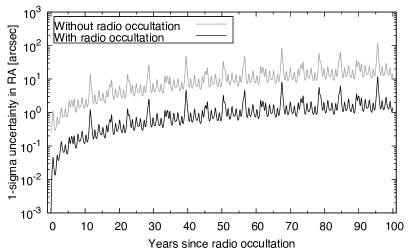
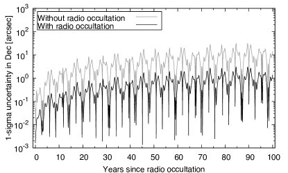
Figure 9: Ephemeris uncertainty for (372) Palma for 100 years subsequent to the occultation in (top) R.A. and (bottom) decl. for a hypothetical geocentric observer. The black line refers to the prediction that includes the occultation-based astrometry, whereas the gray line is a reference that does not include information about the occultation. The long-term trend in the ephemeris uncertainty is caused by the increasing orbital uncertainty and the short-term fluctuation is caused by the varying distance from the Earth to the asteroid (the peaks correspond to the shortest distances).

The measured apparent coordinates for Palma on 2017 May 15 14:31:19.76 UTC as seen from br-vlba are R.A. 01:44:33.5537 and decl. 27:05:03.125. Both coordinates have an uncertainty of $0\farcs 002$, mostly due to uncertainties in the topocentric distance to Palma and the timing of the closest encounter ($\Delta t_{0}=0.08$ s). The position of 0141+268 is known with an order of magnitude higher accuracy; according to the RFC the uncertainties of the R.A. and decl. coordinates are 0.21 mas and 0.28 mas, respectively. The ephemeris by the Jet Propulsion Laboratory’s HORIZONS system for the observing date is in agreement with the measurement given a 3$\sigma$ ephemeris uncertainty of about $0\farcs 05$. Including the coordinates derived from the radio occultation should reduce the uncertainty of the orbital solution, given that the ephemeris uncertainty is an order of magnitude larger than the measurement uncertainty. To test this hypothesis we computed an orbital solution for Palma with all existing optical astrometry available through the Minor Planet Center (excluding visible-wavelength occultations) and the radio occultation included using the OpenOrb software (Granvik et al., 2009). We deliberately excluded visible-wavelength occultations to get a better understanding of how much improvement can be obtained by adding a single radio occultation measurement to regular astrometry spanning more than a century. We used the linearized least-squares method with outlier rejection and included gravitational perturbations by all 8 planets and the 25 most massive asteroids, as well as first-order relativistic corrections for effects caused by the Sun. For the observational error model we used that by Baer et al. without correlations (Baer et al. 2011; Baer & Chesley 2017). Although the more than 1600 astrometric observations of Palma span more than 120 years (1893 September 29 to 2017 November 09), the addition of a single radio occultation measurement has a non-negligible effect on the uncertainties of the orbital elements (in this particular case, a reduction of up to tens of percent) and reduces the uncertainty of ephemerides by an order of magnitude (Figure 9).

The National Radio Astronomy Observatory is a facility of the National Science Foundation operated under cooperative agreement by Associated Universities, Inc. This work made use of the Swinburne University of Technology software correlator, developed as part of the Australian Major National Research Facilities Programme and operated under licence. J.H.and K.M. acknowledge support from the ERC Advanced Grant No. 320773 “SAEMPL”. M.G. acknowledges support from the Academy of Finland (grant #299543). We thank the anonymous referee for insightful comments that helped to improve this manuscript, Mika Juvela for advicing our use of the Monte Carlo simulation, and Dave Herald for pointing out the results from optical occultation observations.

Appendix A Diffraction Patterns and Occultation Curves from a Contiguously Random Shape

Figure 10 shows an example of a random shape that reproduces the observations reasonably well.

Figure 10: Random shape producing small residuals with $\chi^{2}=2.24$. The ratio of the inscribed and circumscribed radii for this model is $r=0.76$. The panels are the same as those in Fig. 5.

References

- Aime et al. (2013) Aime, C., Aristidi, É., & Rabbia, Y. 2013, in EAS Publications Series, Vol. 59, EAS Publications Series, ed. D. Mary, C. Theys, & C. Aime, 37–58
- Baer & Chesley (2017) Baer, J., & Chesley, S. R. 2017, AJ, 154, 76
- Baer et al. (2011) Baer, J., Chesley, S. R., & Milani, A. 2011, Icarus, 212, 438
- Bus & Binzel (2002) Bus, S. J., & Binzel, R. P. 2002, Icarus, 158, 146
- Carry (2012) Carry, B. 2012, Planet. Space Sci., 73, 98
- Cernicharo et al. (1994) Cernicharo, J., Brunswig, W., Paubert, G., & Liechti, S. 1994, ApJ, 423, L143
- Deller et al. (2011) Deller, A. T., Brisken, W. F., Phillips, C. J., et al. 2011, PASP, 123, 275
- Dunham et al. (1999) Dunham, D., Herald, D., Frappa, E., et al. 1999, Asteroid Occultations V1.0., ,
- Durech et al. (2010) Durech, J., Sidorin, V., & Kaasalainen, M. 2010, A&A, 513, A46
- Gordon et al. (2016) Gordon, D., Jacobs, C., Beasley, A., et al. 2016, AJ, 151, 154
- Granvik et al. (2009) Granvik, M., Virtanen, J., Oszkiewicz, D., & Muinonen, K. 2009, Meteoritics and Planetary Science, 44, 1853
- Hanuš et al. (2011) Hanuš, J., Ďurech, J., Brož, M., et al. 2011, A&A, 530, A134
- Hastings (1970) Hastings, W. K. 1970, Biometrika, 57, 97
- Hazard (1976) Hazard, C. 1976, in Methods of Experimental Physics, Vol. 12 C, Astrophysics. Radio Observations, ed. M. L. Meeks, 92
- Hazard et al. (1967) Hazard, C., Gulkis, S., & Bray, A. D. 1967, ApJ, 148, 669
- Hazard et al. (1963) Hazard, C., Mackey, M. B., & Shimmins, A. J. 1963, Nature, 197, 1037
- Kaasalainen et al. (2001) Kaasalainen, M., Torppa, J., & Muinonen, K. 2001, Icarus, 153, 37
- Kooi et al. (2017) Kooi, J. E., Fischer, P. D., Buffo, J. J., & Spangler, S. R. 2017, Sol. Phys., 292, 56
- Lampton et al. (1976) Lampton, M., Margon, B., & Bowyer, S. 1976, ApJ, 208, 177
- Lehtinen et al. (2016) Lehtinen, K., Bach, U., Muinonen, K., Poutanen, M., & Petrov, L. 2016, ApJ, 822, L21
- Lister et al. (2016) Lister, M. L., Aller, M. F., Aller, H. D., et al. 2016, AJ, 152, 12
- Maloney & Gottesman (1979) Maloney, F. P., & Gottesman, S. T. 1979, ApJ, 234, 485
- Marciniak et al. (2012) Marciniak, A., Bartczak, P., Santana-Ros, T., et al. 2012, A&A, 545, A131
- Masiero et al. (2014) Masiero, J. R., Grav, T., Mainzer, A. K., et al. 2014, ApJ, 791, 121
- Masiero et al. (2012) Masiero, J. R., Mainzer, A. K., Grav, T., et al. 2012, ApJ, 759, L8
- Metropolis et al. (1953) Metropolis, N., Rosenbluth, A. W., Rosenbluth, M. N., Teller, A. H., & Teller, E. 1953, J. Chem. Phys., 21, 1087
- Napier et al. (1994) Napier, P. J., Bagri, D. S., Clark, B. G., et al. 1994, IEEE Proceedings, 82, 658
- Oke (1963) Oke, J. B. 1963, Nature, 197, 1040
- Petrov & Kovalev (2017) Petrov, L., & Kovalev, Y. Y. 2017, MNRAS, 467, L71
- Petrov et al. (2008) Petrov, L., Kovalev, Y. Y., Fomalont, E. B., & Gordon, D. 2008, AJ, 136, 580
- Petrov et al. (2011) —. 2011, AJ, 142, 35
- Roques et al. (2008) Roques, F., Georgevits, G., & Doressoundiram, A. 2008, The Kuiper Belt Explored by Serendipitous Stellar Occultations, ed. M. A. Barucci, H. Boehnhardt, D. P. Cruikshank, A. Morbidelli, & R. Dotson, 545–556
- Roques et al. (1987) Roques, F., Moncuquet, M., & Sicardy, B. 1987, AJ, 93, 1549
- Scheuer (1962) Scheuer, P. A. G. 1962, Australian Journal of Physics, 15, 333
- Schloerb & Scoville (1980) Schloerb, F. P., & Scoville, N. Z. 1980, ApJ, 235, L33
- Schmidt (1963) Schmidt, M. 1963, Nature, 197, 1040
- Thompson et al. (2017) Thompson, A. R., Moran, J. M., & Swenson, G. W. 2017, Very-Long-Baseline Interferometry (Cham: Springer International Publishing), 391–483. https://doi.org/10.1007/978-3-319-44431-4_9
- Trahan & Hyland (2014) Trahan, R., & Hyland, D. 2014, Appl. Opt., 53, 3540
- Ďurech et al. (2011) Ďurech, J., Kaasalainen, M., Herald, D., et al. 2011, Icarus, 214, 652
- von Hoerner (1964) von Hoerner, S. 1964, ApJ, 140, 65
- Withers & Vogt (2017) Withers, P., & Vogt, M. F. 2017, ApJ, 836, 114