Semantic Single-Image Dehazing

Abstract

Single-image haze-removal is challenging due to limited information contained in one single image. Previous solutions largely rely on handcrafted priors to compensate for this deficiency. Recent convolutional neural network (CNN) models have been used to learn haze-related priors but they ultimately work as advanced image filters. In this paper we propose a novel semantic approach towards single image haze removal. Unlike existing methods, we infer color priors based on extracted semantic features. We argue that semantic context can be exploited to give informative cues for (a) learning color prior on clean image and (b) estimating ambient illumination. This design allowed our model to recover clean images from challenging cases with strong ambiguity, e.g. saturated illumination color and sky regions in image. In experiments, we validate our approach upon synthetic and real hazy images, where our method showed superior performance over state-of-the-art approaches, suggesting semantic information facilitates the haze removal task.

1 Introduction

Images taken in hazy/foggy weather are generally subject to visibility degradation caused by particle-scattered light, this includes color shifting, contrast loss and saturation attenuation, etc., which may in turn jeopardize the performance of high-level computer vision tasks, e.g. object recognition/classification, aerial photography, autonomous driving and remote sensing.

Existing dehazing algorithms follow a well-received particle model [1], which correlates scene structure and haze-free image under given hazy inputs. Early research make use of multiple images of the same scene taken from different angles/positions to recover structural information and consequently, haze concentration. Single image dehazing, on the other hand, is an extremely ill-posed problem. The challenge arises from the fact that a single hazy image is not informative on scene structure nor clean scene, whereas one is needed to infer the other, causing an ambiguity in clean image estimation. Generally, traditional methods [2, 3, 4] explicitly leverage priors (or constraints) on both fronts: local depth coherence is often assumed, and so is one or more color priors. Recently, several CNN models were proposed for dehazing [5, 6, 7], and have been found on comparable level with prior arts in term of performance. These models are generally light-weighted, and essentially leverage mostly lower level features as dehaze is still considered as an image processing problem.

In a word, existing methods are solely relying on handcrafted physical or low-level priors. While these empirical priors work generally well, one can easily make counterexamples which violate their assumptions (e.g. bright surface, colored haze). A well-observed problem with this is that the restored image tends to be over-saturated and has incorrect tone. This problem is in general unsolvable based on the insufficient low-level information alone. However, human users can easily tell the naturalness of color, e.g. whether the tree is too green or the sky is too blue. Such feeling is not from any low-level priors but rather because of the semantic prior that we humans have a knowledge about.

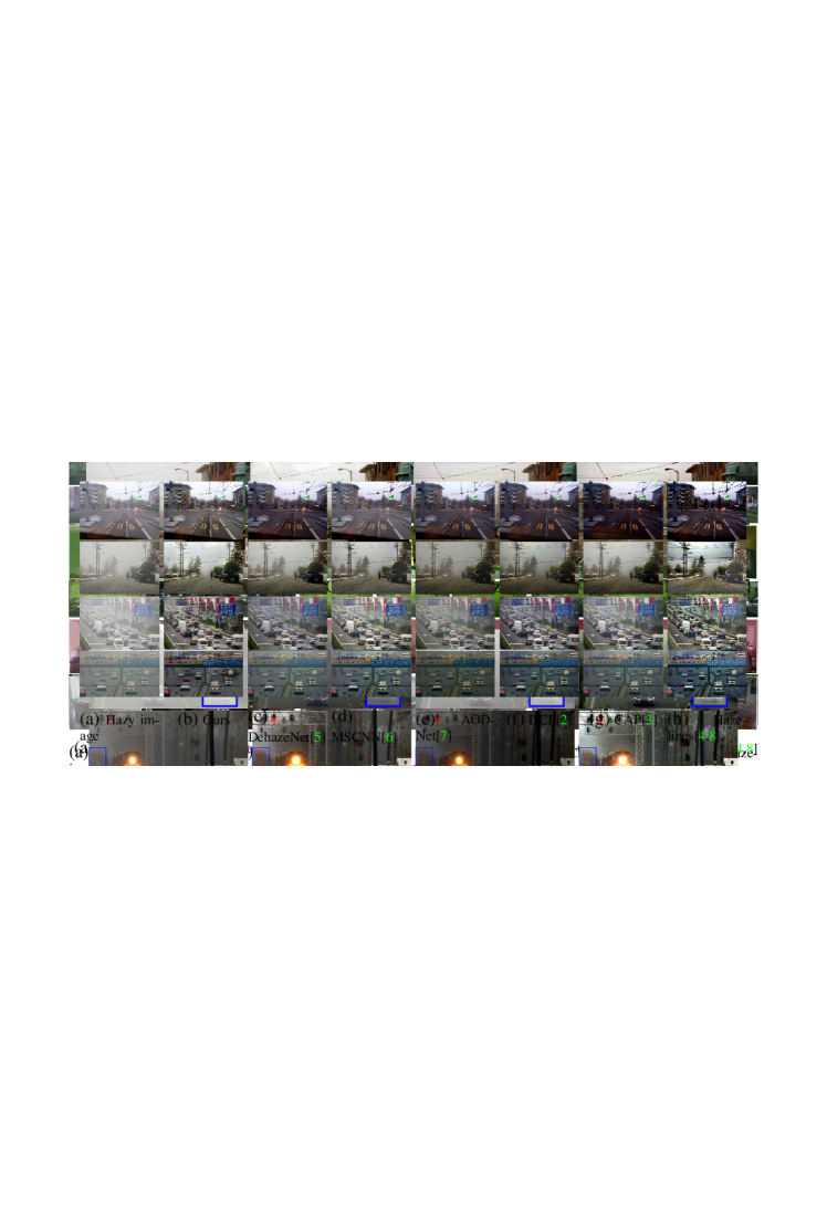
Figure 1: The proposed semantic solution towards dehazing: we rely on semantic priors to provide additional information that is otherwise hard to obtain. This extra knowledge can be helpful with predicting objects’ true color as well as ambient illumination.

In this paper we introduce semantics-based dehazing, a novel method that uses semantic information to provide additional guidance for inferring clean image. Semantic clues have seen success in other ‘low-level’ applications, e.g. color constancy [9] and image filtering [10]. Here we propose a fully end-to-end convolutional neural network (CNN) that learns the correlation between semantics and objects’ natural color from training samples, and infer the clean scene and illumination color based on learned semantic features. As such, for object class of medium or strong semantic color prior (e.g. sky is blue and vegetations are green), the semantics provides informative cues on the object’s true color, and the clean scene and ambient illumination can be learned with high confidence; for objects of medium or weak semantic prior, the true color can be predicted with, for example, low-level priors and ambient illumination estimation from other strongly confident objects. The conceptual idea behind our approach is illustrated in Figure 1.

The main contribution of this paper is that we are the first to explicitly exploit high-level features to provide informative color priors for single image haze removal problem. We found that our approach is robust against extreme settings (bright surfaces, severe color shifting, saturated atmospheric light, sky regions etc.) which impose major challenges on previous methods. We show in experiments that the proposed model obtains state-of-the-art results on RGB-D testsets with synthetic haze. As the model is trained on street scenes, we also test our model on real world hazy scenes of similar semantic classes, where the model shows comparable results with state-of-art methods.

2 Related work

2.1 Atmospheric scattering model

Following [1], hazy imagery can be seen as the linear combination of true object color and ambient illumination (Figure 3), hence the equation

$$I(x)=J(x)\,t(x)+A\,\big{(}1-t(x)\big{)}\text{,}$$ (1)

where $I(x)$ is the hazy image value for pixel $x$, $J(x)$ is the corresponding clean image, $A$ is the color of ambient illumination, and $t(x)\in(0,1]$ represents the transmission. Assuming the haze is uniformly distributed in space, the transmission $t(x)$ is defined as

$$t(x)=e^{-\beta\,d(x)}\text{,}$$ (2)

where $d(x)$ is the object distance from camera center and $\beta$ a non-negative scattering coefficient related to haze particles.

Figure 2: Mount Baker from distance in different weather (taken from Internet). Clean image (left) and two different illumination colors (middle and right) are stitched together.

Sometimes it is assumed that $A$ is a bright gray/white color [3, 6, 5]. However, with some particles or specific lighting conditions, $A$ may take other color as well (e.g. yellow/red), as illustrated in Figure 2.

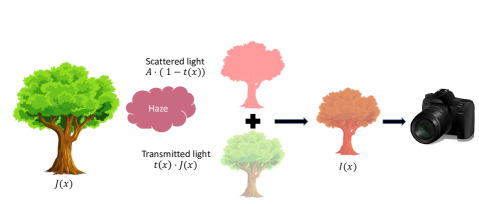
Figure 3: Atmospheric scattering model. The captured image is a convex combination of ambient illumination and clean scene.

2.2 State-of-the-art for haze removal

While there have been many developments in single image dehazing (e.g. maximal local contrast [11], atmospheric light recovery [12], learning framework for haze features [13], color-line [14], artifacts removal for compressed hazy image and video [15]), in this section we will only list some of the most prominent or recent ones. For a comparative survey of other existing dehazing algorithms, we refer the reader to [16].

Dark channel prior (DCP) [2] is based on the observation that at least one of RGB channels of real world objects often has a very small value. Under this assumption, the color shifting caused by ambient illumination can be obtained by its dark channel, hence the transmission. Color attenuation prior (CAP) [3] by Zhu et al. creates a linear model correlating scene depth and the difference between local saturation and brightness. Haze-line [4, 8] assumes that real world images have distinct colors so that image pixels form clusters in RGB space. With the presence of haze, the clusters are shifted towards ambient illumination based on transmission forming so-called haze-lines. Recently some deep learned methods have also been proposed. DehazeNet [5] employs an end-to-end fully convolutional network (FCN) [17] to learn the scene transmission. However, the network is trained on small image patches with constant transmission per patch, and does not factor in non-local features. MSCNN Dehaze [6] propose a multi-scale CNN for learning a coarse transmission, and relies on another CNN in the pipeline for refining it. AOD-Net [7] is the first end-to-end model to directly produce clean images, and has been found to boost the performance for high-level vision tasks under hazy weather conditions. Yang et al. [18] design three separate networks to generate the clean image, ambient illumination and transmission respectively and use an adversarial network for semi-supervised learning.

As image dehazing is generally considered a low-level task, existing dehaze algorithms seek priors from either empirical observations or the physical haze model. While deep learned technologies do not explicitly assume such knowledge, they are light-weighted and are ultimately designed to learn low-level haze-related features.

2.3 Datasets for single image dehazing

Since it is difficult to take images under different weather conditions while keeping other scene settings unchanged, currently there is no dataset offering a large number of real world hazy images and the corresponding clean images.

Previous hazy datasets uniformly synthesize haze on RGB-D images based on (1). Due to the difficulty of collecting depth map in outdoor settings, most RGB-D datasets contain indoor scenes only (e.g. D-Hazy dataset [19], which use images and depth maps from NYU [20] and Middlebury [21, 22, 23] datasets). Depth maps for outdoor scenes are in general less accurate and are obtained by (a) view disparity from stereo cameras (e.g. FoggyCityscapes [24]) or (b) monocular image depth estimation (e.g. RESIDE [25] used [26] to generate depth maps). Apart from that, all existing synthetic hazy datasets use illumination color close to grayscale, the only exception being Fattal’s dataset [14], which selects sky color as illumination color.

3 Semantic color prior

We proposed a novel method that explores semantics for dehazing by training a CNN model to learn from training set the color distribution conditioned on a set of semantic features. This approach allows our model to infer semantic priors for recovering true scene color. The extra knowledge obtained with semantic cues is used to remedy the lack of information in a single image when the model sees similar semantics again.
Clean image: Conventional methods rely on the physical haze model to restore the true color of an object. This requires an accurate estimation of the atmospheric light and transmission value (structural information), both are difficult to obtain. However, there often exists a strong correlation between a semantic class and the color distribution it exhibits (e.g. vegetations are likely to have green color), as such, the true color can sometimes be predicted directly with a high confidence (see Figure 1). The semantic features thus can offer a strong prior for the prediction of clean image which can be particularly useful when the estimation ambiguity is high (e.g. very small transmission value). An example is the sky region with effectively infinite depth, in which case it is impossible to recover the true color. However, when correctly identified as sky, the image part is likely to be colors of blue hue. Although the guess is not necessarily accurate, a color distribution can nonetheless be learned and exploited to reduce the ambiguity of prediction.
Ambient illumination: On the other hand, semantic context can also be useful for estimating atmospheric illumination color, the most straightforward case also being the sky regions, which often have color close to ambient light. This may in turn benefit objects with weak semantic priors (e.g. cars can be of arbitrary color, but a car spatially adjacent to road or tree will likely have similar depth and transmission, and its true color may then be inferred given ambient illumination, as illustrated in Figure 1).

In practice, however, we also observe that objects’ true color and ambient illumination are mutually dependent when given hazy image as input. Consequently, we design a network to incorporate them both and allow one to refine the other. Instead of asking our network to explicitly predict illumination color, we make use of a set of global features, which may carry global contextual information related to e.g. not only ambient illumination color but also global scene semantics. This non-locality allows information learned from objects of strongly confident semantic priors to propagate to other parts of the image, and benefit the true color prediction for objects with weak semantic priors.

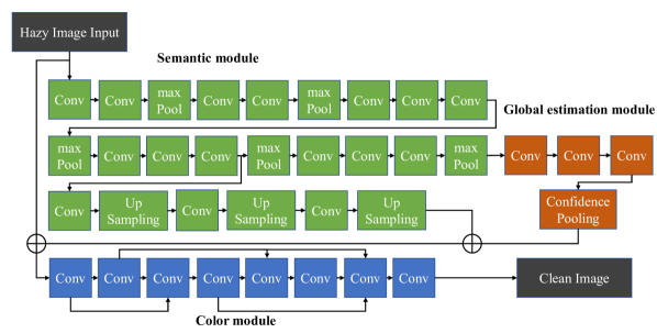
Figure 4: Pipeline of the proposed model consists of a semantic module, a global estimation module and a color module (colored in green, orange, and blue respectively). Note that the outputs from both semantic module and global estimation module are up-sampled/broadcast to original images size, and concatenated with hazy image as inputs to color module.

3.1 Overview

The pipeline of the proposed model is illustrated in Figure 4. The model takes hazy images as input and the output is the predicted clean image. Our model, following a fully convolutional design, consists of three modules: a semantic module for higher-level semantic feature extraction, a global estimation module for predicting global features, and finally a color module for inferring clean image.

3.2 Semantic module

For semantic feature extraction, we exploit a well-known image classification network VGG16 [27] that is pre-trained on ImageNet dataset [28]. The model has been extensively trained for object recognition task over 1,000 semantic categories [28]. As we only need the semantics-related features rather than the exact labeling, we remove the final dense and softmax layer of the VGG model, and use the output of its intermediate convolutional layers for semantic feature extraction. We chose VGG16 for its good performance and simplicity in design. VGG16 model has 5 multilayer blocks (which we call block 1 to block 5), each has several convolutional layers followed by one max pooling layer [27]. Since we want to enforce the generalizability of semantic network, we do not train the VGG model to serve our dataset, i.e. its weights are fixed during training.

It is commonly observed that as information propagates through deep CNN (e.g. classification and recognition models), the processed knowledge generally becomes less informative but more task-oriented. In order to balance the trade-off between information loss and the task-specificness (which in this case is scene semantics extraction), we use the final convolution layer in block 4 of VGG16 (down-sampled by a factor of 8) for local features to infer color priors. The extracted local semantic features are then up-sampled to original image size by a light-weighted three-stage subnet to accommodate the input size of color module. In each stage, the number of features is reduced by half using a convolutional layer with kernel size $3\times 3$, and the feature maps are then up-sampled by a factor of 2.

3.3 Global estimation module

We further exploit the semantic module for estimating a set of 32 global features . The key intuition behind this design is that global features may carry valuable information about ambient illumination or semantic context, which can be inferred from scene semantics. The block 5 output of the VGG16 model (down-sampled by a factor of 32) is sent to our global estimation module which predicts a single value ($1\times 1$ size feature) for each feature map.

We adopt the confidence-weighted pooling technique proposed in [9]. The proposed global estimation module is trained to learn from each input patch $\Omega$ a set of local features ${\cal{F}}_{\Omega}$, as well as the local confidence $C_{\Omega}$. The global features $\cal{F}$ is then obtained by averaging local features weighted by their individual confidence:

$${\cal{F}}=\frac{1}{\sum_{\Omega}C_{\Omega}}\sum_{\Omega}{\cal{F}}_{\Omega}\cdot C_{\Omega}\text{.}$$ (3)

This pooling technique enables our model to extract global features depending on the confidence level of semantic priors on local regions, as some semantic classes may have higher significance than others (as shown in Figure 1). The global pooling allows local features to be aggregated and broadcast to other part of image, and effectively enables image-sized receptive field in a fully convolutional architecture.

To this end we build a light-weight model with four intermediate layers to learn global features. We use the first three convolutional layers (of filter size $5\times 5\times 256$, $5\times 5\times 64$ and $1\times 1\times 33$ respectively) for further feature extraction. The input to confidence pooling layer has $33$ features, where the first $32$ are the predicted local features and the last feature is the corresponding confidence. A layer-wise softmax activation is applied on confidence for normalization purpose before pooling. The final output of global estimation module is reduced to a $1\times 1$ feature map of $32$ channels.

3.4 Color module

The color module reads in both semantic features and global features. The global features are broadcast to original image size, at which point the hazy image and semantic and global feature maps are concatenated, as illustrated in Figure 4.

The concatenated inputs are then processed by our color module. For this part, we use the architecture of AOD-Net [7] since it is the state-of-art end-to-end CNN dehazing model. However, in our case, the input contains not only hazy images, but also a $48$-channel feature map ($16$ for semantic features and $32$ for global features), and consequently, intermediate layers have more filters to process the additional input features. The original AOD-Net has $3$ filters for each of its $5$ convolutional layers and our modified version has $16$, $16$, $8$, $4$, $3$ filters respectively. No other modifications were done. The final output of our network is an RGB image of predicted clean scene.

4 Experiment Evaluations

We conduct extensive experiments, to evaluate the performance of the proposed method. We compare our model both qualitatively and quantitatively against other existing methods on both synthetic and real hazy images. We are also interested in testing under some challenging settings, e.g. non-grayscale illumination color and/or very small transmission values — both cause estimation ambiguity. Finally, we conduct ablation study to compare our model with a baseline implementation without semantic information.

4.1 Datasets

Considering that the indoor settings may not be applicable for hazy scenes and indoor and outdoor images contain different semantic classes, in our experiments, we combine the labeled NYU/NYU2 [20, 29] and the Cityscapes [30] datasets for training and testing. All images are resized to $256\times 256$ pixels to fit the input size of the pre-trained VGG16 model. We do not include Middlebury dataset for testing because Middlebury has limited depth range and different semantic classes from NYU/NYU2; RGB datasets with learned depth (e.g. RESIDE) are not considered for training or testing either as their depth prediction often suffers poor quality.

The hazy dataset used in this paper is generated from the RGB-D images following the physical model in (1) and (2). The Cityscapes dataset does not provide depth map, and the depth information is instead given in the form of disparity maps. As such, the depth for Cityscapes is calculated inversely proportional to the disparity values, i.e. the transmission is obtained from $e^{-\frac{\beta}{D}}$ where $D$ is the disparity value. To handle occlusions, we first crop the Cityscapes images so the left and bottom margins with most occluded parts are removed. We then adopt the nearest neighbor assignment approach [31] to fill in the missing values for remaining occluded pixels.

The RGB-D datasets used in our experiments are split for training and testing purposes as shown in Table 1.

Table 1: Breakdown of unique RGB-D images for training and testing purposes

Dataset	Training		Testing		Total
	train	validation	testsetA	testsetB
NYU	1524	152	608		2284
NYU2	969	96	384		1449
Cityscapes	2575	400	1525	0	4500
Total	5068	648	2517	992	8233

The training and testing hazy images are synthesized using the RGB-D images, random illumination colors and different haze coefficients. As real world haze may exhibit non-gray colors, we sample the illumination color from HSV color space. In our experiments we use a lightness value (i.e. the value of V in HSV) from $U(0.6,1)$ and saturation from $U(0,0.5)$ (where $U$ stands for uniform distribution). The hue is sampled in full range of $U(0,1)$ since there is no prior knowledge on it. For NYU and NYU2 dataset, the haze coefficient $\beta$ is uniformly in $\{0.1,0.2,0.3,0.4\}$ (unit is $m^{-1}$) and for Cityscapes it is uniformly in $\{5,7.5,12.5,20\}$ (unit is the disparity unit) .

From each of the 2,517 RGB-D images in the test set we generate $4$ hazy images using different $\beta$ and a random illumination color as described above. We call this testsetA. Since NYU/NYU2 datasets are widely used for quantitative evaluation in the single image dehaze literature [25, 19], for better comparability, we construct another testsetB, which is synthesized using only test images from NYU and NYU2 in Table 1 and contains a totality of 3,968 hazy images. For each RGB-D image and $\beta$, we generate one hazy image with grayscale illumination color (illumination color is from HSV space with $S=0$ and $V$ from $U(0.6,1)$).

4.2 Training setup

We train our model on the RGB-D training set using haze generation scheme described above. The training inputs are shuffled for each epoch and batched to size of $8$. The model is trained with Adam optimizer [32] at learning rate of $1e-4$ and default momentums. After each epoch we evaluate the model on the validation set. An early stop criterion applies when training loss has converged and the best validation loss has not improved over $7$ consecutive epochs.

Given the massive amount of used RGB-D images, instead of keeping a static hazy dataset like we did before with testsetA and testsetB, we generate the training and validation hazy images on the fly. During every epoch we loop over all RGB-D images and for each image with each pre-defined haze coefficient, generate one pair of hazy/clear scene with randomly sampled illumination colors. In this way, we increase the diversity of training samples by not reusing pre-stored hazy images.

4.3 Quantitative evaluation

We compare our model with the state-of-art methods described in section 2.2 on synthetic hazy images. For that we use the mean squared error (MSE), peak signal to noise ratio (PSNR) and structural similarity (SSIM) metrics. Since [18] did not publicize their source code or trained model, we do not include it for comparison.

The results listed in Table 2 and 3 are evaluated on testsetA and testsetB, respectively. Given the large number of test images, we use the default optimal parameters reported in the corresponding papers or implementations for comparing state-of-art methods. In both Table 2 and 3, our method produces significantly better results than existing methods, suggesting that the semantic prior is a powerful tool for image dehazing.

Table 2 shows that our method is robust against the estimation ambiguity introduced by different illumination settings. Since the illumination is not on grayscale, handcrafted priors such as CAP are violated. Previous CNN methods also do not perform well under this settings, because (a) they are light-weighted model with limited learning capacity as they are designed to learn only low-level features and (b) they are trained on less challenging dataset with only grayscale haze scenes. On testsetB, however, CNN approaches generally have better performance than hand-crafted priors (except for DCP [2]). Interestingly, while Haze-lines [4, 8] has the lowest score on PSNR metric, it has the second best score on SSIM in Table 2. This is in line with our later observation where Haze-lines shows noticeably better image quality than other existing methods .

Table 2: Comparison with the state-of-art methods over SSIM, PSNR (larger is better) and MSE (lower is better) metrics on synthetic hazy images in our testsetA with color scale haze. CNN models are listed on the left and handcrafted priors methods are listed on the right.

Metrics	Ours	DehazeNet[5]	MSCNN[6]	AOD-Net[7]	DCP[2]	CAP[3]	Haze-lines[4, 8]
SSIM	0.9018	0.5829	0.6487	0.5159	0.6329	0.5675	0.6598
MSE	0.0020	0.0311	0.0255	0.0337	0.0243	0.0320	0.0405
PSNR	28.195	16.735	17.075	15.537	17.063	15.752	15.515

Table 3: Comparison with the state-of-art methods over SSIM, PSNR (larger is better) and MSE (lower is better) metrics on synthetic hazy images in testsetB with grayscale haze. CNN models are listed on the left and handcrafted priors methods are listed on the right.

Metrics	Ours	DehazeNet[5]	MSCNN[6]	AOD-Net[7]	DCP[2]	CAP[3]	Haze-lines[4, 8]
SSIM	0.9024	0.8140	0.7621	0.8027	0.8212	0.7744	0.7146
MSE	0.0027	0.0158	0.0217	0.0208	0.0157	0.0215	0.0290
PSNR	27.083	20.291	18.229	18.103	19.391	17.920	16.722

4.4 Qualitative evaluation

In this section we qualitatively compare the results of the proposed model and state-of-art methods over a collection of synthetic and real world hazy images. The images used in this evaluation are taken from our testsetA as well as real world scenes from the Internet and Foggy Driving dataset [24]. Given the semantic-aware nature of our model, the real world scenes for comparison are selected to contain similar semantic classes to the training set.

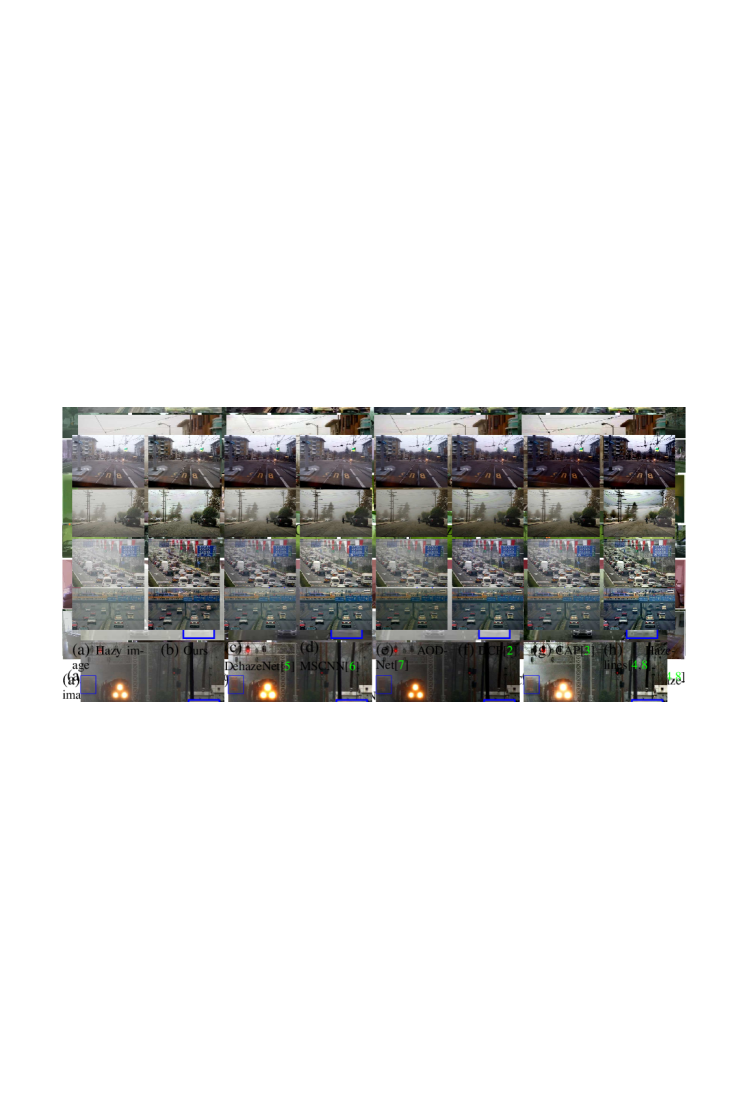
Figure 5: Visual comparison with the state-of-art methods on our testsetA. Images are resized for viewing purpose.

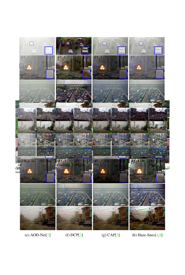
Figure 6: Visual comparison with the state-of-art methods on real world hazy images of urban scenes from Internet and [24].

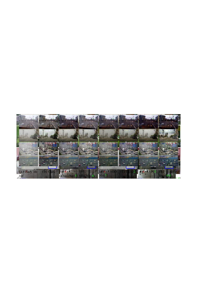
Figure 7: Visual comparison with the state-of-art methods on real world hazy images of urban scenes from Internet and [24].

Figure 5-7 show that our model can recover the scene under very strong haze and restore plausible color to objects indistinguishable to human eyes. One notable example is the sky region in Cityscapes dataset shown in Figure 5. Although the sky has very small transmission values, i.e. it suffers from severe color shift, our model is still able to recover it naturally. In Figure 6, the images with medium and strong haze levels are extrapolated properly, and the brightness and color balance restored. The trees in the top row appear green and our method produces less artifacts than DCP and Haze-Lines.

On the other hand, existing methods are susceptible to over-saturation, especially when illumination color is not on grayscale. A noticeable example is the predicted image by DCP [2] in Figure 5, where the saturation is apparently increased, causing color shifts even more from the clean scene seen in ground truth images. Among existing methods, Haze-lines [4] has arguably the best visual quality in Figure 6, when other existing methods fail to properly restored white balance or fully lift the haze in the image.

This gap in visual quality is mainly because the semantic approach enables our model to understand what is being imaged, which provides informative priors that are otherwise impossible to learn from lower-level features alone.

4.5 Ablation study

To further validate the proposed semantic approach, we compare our model with a baseline that receives no semantic features. In this ablation study we aim to exam the semantic dependency of our method and how that would impact performance. To this end, we remove the semantic-related features by isolating the color module from the rest of the pipeline, i.e. both semantic module and global estimation module are dropped out from the design.

Since the semantic and global estimation modules may learn to predict illumination-related features as well as semantic features, here we use the same dataset introduced before, but with ground truth RGB ambient illumination color as additional input when training and testing. We concatenate the hazy image with illumination color to form a 6-channel input (as opposed to the 51-channel input of original color module). To ensure that this does not undermine the model’s learning capacity, the number of filters in the first convolutional layer is increased to $24$ so the baseline has slightly more parameters than the original color module. Otherwise there is no difference between the baseline and our original color module. For fair comparison we train the baseline model with the same dataset and training routine described before.

Table 4: Comparison of baseline and the proposed method over different metrics on testsetA. Both models are trained and tested on the same dataset.

Method	SSIM	MSE	PSNR
Ours	0.9024	0.0020	27.0827
Baseline	0.7762	0.0061	23.2918

Table 4 shows the performance of baseline over testsetA. The performance varies considerably from the baseline to our semantic approach even when we provide additional ground truth illumination color to the former. Note that although the baseline shares the same layer architecture with AOD-Net [7], it still wins by a large margin over our test set. This is because (a) the baseline is trained on more challenging dataset with non-grayscale ambient illumination (b) the baseline has more filters (parameters) than AOD-Net and (c) ground truth illumination is known to the baseline model but not to AOD-Net.

5 Conclusion and discussions

In this paper we introduced a semantic approach towards single image dehazing. We are the first to explicitly exploit semantic features for learning semantic priors which are used to provide informative priors for estimating underlying clean scene. We achieved state-of-the-art performance on synthetic hazy images and our model is able to accurately recover clean scene under strong estimation ambiguity, e.g. strong haze and semi-saturated ambient illumination, with learned semantic priors.

Due to the difficulty for acquiring real world training data, our dataset contains only indoor scenes and outdoor road scenes, which implies a deficit for semantics of general real world objects as well as their corresponding real colors. Therefore, it is challenging to learn semantic-color priors for real world outdoor objects that are not seen during training, which means we cannot show our model can generalize well to natural outdoor scenes until relevant datasets are made available. This limitation is on the published data rather than on our methodology, and the generalizability is traded for much higher accuracy seen in experiments. In future we will improve this by training our model with a wider range of images.

6 Acknowledgement

We would like to thank Christos Sakaridis for his careful review of our paper which helped improve its quality.

References

- [1] S. G. Narasimhan and S. K. Nayar, “Contrast restoration of weather degraded images,” IEEE transactions on pattern analysis and machine intelligence, vol. 25, no. 6, pp. 713–724, 2003.
- [2] K. He, J. Sun, and X. Tang, “Single image haze removal using dark channel prior,” IEEE transactions on pattern analysis and machine intelligence, vol. 33, no. 12, pp. 2341–2353, 2011.
- [3] Q. Zhu, J. Mai, and L. Shao, “A fast single image haze removal algorithm using color attenuation prior,” IEEE Transactions on Image Processing, vol. 24, no. 11, pp. 3522–3533, 2015.
- [4] D. Berman, S. Avidan, et al., “Non-local image dehazing,” in Proceedings of the IEEE conference on computer vision and pattern recognition, pp. 1674–1682, 2016.
- [5] B. Cai, X. Xu, K. Jia, C. Qing, and D. Tao, “Dehazenet: An end-to-end system for single image haze removal,” IEEE Transactions on Image Processing, vol. 25, no. 11, pp. 5187–5198, 2016.
- [6] W. Ren, S. Liu, H. Zhang, J. Pan, X. Cao, and M.-H. Yang, “Single image dehazing via multi-scale convolutional neural networks,” in European Conference on Computer Vision, pp. 154–169, Springer, 2016.
- [7] B. Li, X. Peng, Z. Wang, J. Xu, and D. Feng, “Aod-net: All-in-one dehazing network,” in Proceedings of the IEEE International Conference on Computer Vision, 2017.
- [8] D. Berman, T. Treibitz, and S. Avidan, “Air-light estimation using haze-lines,” in 2017 IEEE International Conference on Computational Photography (ICCP), pp. 1–9, May 2017.
- [9] Y. Hu, B. Wang, and S. Lin, “Fc 4: Fully convolutional color constancy with confidence-weighted pooling,” in Proceedings of the IEEE Conference on Computer Vision and Pattern Recognition, pp. 4085–4094, 2017.
- [10] Q. Yang, “Semantic filtering,” in Proceedings of the IEEE Conference on Computer Vision and Pattern Recognition, pp. 4517–4526, 2016.
- [11] R. T. Tan, “Visibility in bad weather from a single image,” in Computer Vision and Pattern Recognition, 2008. CVPR 2008. IEEE Conference on, pp. 1–8, IEEE, 2008.
- [12] M. Sulami, I. Glatzer, R. Fattal, and M. Werman, “Automatic recovery of the atmospheric light in hazy images,” in Computational Photography (ICCP), 2014 IEEE International Conference on, pp. 1–11, IEEE, 2014.
- [13] K. Tang, J. Yang, and J. Wang, “Investigating haze-relevant features in a learning framework for image dehazing,” in Proceedings of the IEEE Conference on Computer Vision and Pattern Recognition, pp. 2995–3000, 2014.
- [14] R. Fattal, “Dehazing using color-lines,” vol. 34, (New York, NY, USA), ACM, 2014.
- [15] C. Chen, M. N. Do, and J. Wang, “Robust image and video dehazing with visual artifact suppression via gradient residual minimization,” in European Conference on Computer Vision, pp. 576–591, Springer, 2016.
- [16] Y. Li, S. You, M. S. Brown, and R. T. Tan, “Haze visibility enhancement: A survey and quantitative benchmarking,” Computer Vision and Image Understanding, 2017.
- [17] J. Long, E. Shelhamer, and T. Darrell, “Fully convolutional networks for semantic segmentation,” in Proceedings of the IEEE Conference on Computer Vision and Pattern Recognition, pp. 3431–3440, 2015.
- [18] X. Yang, Z. Xu, and J. Luo, “Towards perceptual image dehazing by physics-based disentanglement and adversarial training,” 2018.
- [19] C. Ancuti, C. O. Ancuti, and C. D. Vleeschouwer, “D-hazy: A dataset to evaluate quantitatively dehazing algorithms,” in 2016 IEEE International Conference on Image Processing (ICIP), pp. 2226–2230, Sept 2016.
- [20] N. Silberman and R. Fergus, “Indoor scene segmentation using a structured light sensor,” in Proceedings of the International Conference on Computer Vision - Workshop on 3D Representation and Recognition, 2011.
- [21] J. Zbontar and Y. LeCun, “Stereo matching by training a convolutional neural network to compare image patches,” Journal of Machine Learning Research, vol. 17, no. 1-32, p. 2, 2016.
- [22] D. Scharstein and C. Pal, “Learning conditional random fields for stereo,” in Computer Vision and Pattern Recognition, 2007. CVPR’07. IEEE Conference on, pp. 1–8, IEEE, 2007.
- [23] D. Scharstein and R. Szeliski, “High-accuracy stereo depth maps using structured light,” in Computer Vision and Pattern Recognition, 2003. Proceedings. 2003 IEEE Computer Society Conference on, vol. 1, pp. I–I, IEEE, 2003.
- [24] C. Sakaridis, D. Dai, and L. Van Gool, “Semantic foggy scene understanding with synthetic data,” ArXiv e-prints, 2017.
- [25] B. Li, W. Ren, D. Fu, D. Tao, D. Feng, W. Zeng, and Z. Wang, “Reside: A benchmark for single image dehazing,” arXiv preprint arXiv:1712.04143, 2017.
- [26] F. Liu, C. Shen, G. Lin, and I. Reid, “Learning depth from single monocular images using deep convolutional neural fields,” IEEE Transactions on Pattern Analysis and Machine Intelligence, vol. 38, pp. 2024–2039, Oct 2016.
- [27] K. Simonyan and A. Zisserman, “Very deep convolutional networks for large-scale image recognition,” arXiv preprint arXiv:1409.1556, 2014.
- [28] O. Russakovsky, J. Deng, H. Su, J. Krause, S. Satheesh, S. Ma, Z. Huang, A. Karpathy, A. Khosla, M. Bernstein, A. C. Berg, and L. Fei-Fei, “ImageNet Large Scale Visual Recognition Challenge,” International Journal of Computer Vision (IJCV), vol. 115, no. 3, pp. 211–252, 2015.
- [29] N. Silberman, D. Hoiem, P. Kohli, and R. Fergus, “Indoor segmentation and support inference from rgbd images,” Computer Vision–ECCV 2012, pp. 746–760, 2012.
- [30] M. Cordts, M. Omran, S. Ramos, T. Rehfeld, M. Enzweiler, R. Benenson, U. Franke, S. Roth, and B. Schiele, “The cityscapes dataset for semantic urban scene understanding,” in Proc. of the IEEE Conference on Computer Vision and Pattern Recognition (CVPR), 2016.
- [31] S. Huq, A. Koschan, and M. Abidi, “Occlusion filling in stereo: Theory and experiments,” vol. 117, p. 688–704, 06 2013.
- [32] D. P. Kingma and J. Ba, “Adam: A method for stochastic optimization,” CoRR, vol. abs/1412.6980, 2014.