Parafermionic generalization of the topological Kondo effect

Abstract

We propose and study a parafermionic generalization of the topological Kondo effect. The latter has been predicted to arise for a Coulomb-blockaded mesoscopic topological superconductor (Majorana box), where at least three normal leads are tunnel-coupled to different Majorana zero modes on the box. The Majorana states represent a quantum impurity spin that is partially screened due to cotunneling processes between leads, with a stable non-Fermi liquid ground state. Our theory studies a generalization where (i) Majorana states are replaced by topologically protected parafermionic zero modes, (ii) charging effects again define a spin-like quantum impurity on the resulting parafermion box, and (iii) normal leads are substituted by fractional edge states. In this multi-terminal problem, different fractional edge leads couple only via the parafermion box. We show that although the linear conductance tensor exhibits similar behavior as in the Majorana case, both at weak and strong coupling, our parafermionic generalization is actually not a Kondo problem but defines a rich new class of quantum impurity problems. At the strong-coupling fixed point, a current injected through a reference lead will be isotropically partitioned into outgoing currents in all other leads, together with a universal negative current scattered into the reference lead. The device can thus be operated as current extractor, where the current partitioning is noiseless at the fixed point. We describe a fractional quantum Hall setup proximitized by superconductors and ferromagnets, which could allow for an experimental realization in the near future.

I Introduction

A major goal of modern condensed matter physics is to understand and predict the physics of Majorana zero modes Alicea2012 ; Leijnse2012 ; Beenakker2013 ; Lutchyn2018 and their generalizations such as parafermionic zero modes Nayak2008 ; Alicea2016 . Apart from the fundamental interest in observing, manipulating, and controlling exotic fractionalized excitations, quantum states encoded by sets of zero modes with non-Abelian braiding statistics hold significant promise for quantum information processing applications due to their topologically protected and highly nonlocal character Nayak2008 ; Sarma2015 . While experimental evidence for Majorana states is rapidly mounting in different platforms Mourik2012 ; Deng2012 ; Das2012 ; Rokhinson2012 ; Yazdani2014 ; Franke2015 ; Sun2016 ; Albrecht2016 ; Deng2016 ; Guel2017 ; Zhang2017 ; Albrecht2017 ; Nichele2017 ; Suominen2017 ; Gazi2017 ; Feldman2017 ; Deacon2017 , experimental searches for condensed-matter realizations of parafermions (PFs) with symmetry $\mathbb{Z}_{n>2}$ are just about to start Ronen2018 ; Wu2018 . (Note that $\mathbb{Z}_{2}$ PFs reduce to Majorana zero modes.)

The theoretical understanding of PFs, on the other hand, is already comparatively well advanced, and many interesting phenomena have been predicted Alicea2016 ; Lindner2012 ; Cheng2012 ; Clarke2013 ; Burrello2013 ; Vaezi2013 ; Zhang2014 ; Mong2014 ; Clarke2014 ; Barkeshli2014a ; Barkeshli2014b ; Klinovaja2014 ; Klinovaja2014b ; Cheng2015 ; Alicea2015a ; Kim2017 ; Snizhko2018 ; Pachos2018 ; Chew2018 . While it has recently been shown that $\mathbb{Z}_{4}$ PFs admit a free-fermion description Pachos2018 ; Chew2018 , theoretical constructions for more general cases usually exploit the competition between different gapping mechanisms at edge states of a topologically ordered two-dimensional phase. Suggested platforms for hosting PF zero modes include bilayer fractional quantum Hall (FQH) systems Barkeshli2014b , proximitized fractional topological insulators Lindner2012 , and proximitized FQH liquids at filling factor $\nu=2/3$ Mong2014 or $\nu=1/(2k+1)$ with integer $k$ Lindner2012 ; Clarke2013 . Such setups have, in principle, the potential to ultimately realize Fibonacci anyons capable of topologically protected universal quantum computations Mong2014 ; Alicea2015a . In particular, opposite-spin FQH edges proximitized by alternating domains of superconductors (SCs) and ferromagnets (FMs) should trap stable PF zero modes at domain walls Lindner2012 . We note that recent experimental progress has demonstrated that the seemingly conflicting requirements of high magnetic fields (for the FQH phase) and superconductivity in principle can be reconciled Lee2017 ; Lee2017a .

In the present work, we analyze a previously unnoticed aspect of PFs arising in the presence of Coulomb charging effects. In fact, recent theoretical Fu2010 ; Zazunov2011 ; Hutzen2012 and experimental Albrecht2016 work has highlighted the importance of Coulomb charging effects in a floating mesoscopic superconductor hosting Majorana bound states (‘Majorana box’). By gapping out charge degrees of freedom and by blocking detrimental processes related to quasiparticle poisoning Aasen2016 ; Plugge2016 , a large box charging energy $E_{C}$ can further stabilize the Majorana subsector of the Hilbert space. Importantly, charging effects will also activate long-range cotunneling processes between different leads (or other access elements) attached to the box via tunnel contacts. Consequently, Majorana boxes are key ingredients for recently proposed topological quantum information processing schemes Plugge2016 ; Landau2016 ; Plugge2017 ; Karzig2017 ; Litinski2017 . When the Majorana box is operated under Coulomb valley conditions, with $M\geq 3$ normal-conducting (effectively spinless) leads tunnel-coupled to Majorana zero modes on the box, the Majorana sector becomes equivalent to an effective quantum impurity spin with SO$(M)$ symmetry Beri2012 . For the minimal case with $M=3$, this impurity spin corresponds to a standard spin-$1/2$ operator $(\hat{s}_{x},\hat{s}_{y},\hat{s}_{z})$, where distinct operator components are nonlocally represented by different Majorana bilinears on the box. Noting that also the leads have SO$(M)$ symmetry, cotunneling processes between different leads then act like an exchange coupling and thus partially screen the effective impurity spin. Ultimately, such processes drive the system to a robust non-Fermi liquid fixed point analogous to the overscreened multi-channel Kondo fixed point. For a detailed discussion of this topological Kondo effect (TKE), see Refs. Beri2012 ; Altland2013 ; Beri2013 ; Crampe2013 ; Tsvelik2013 ; Zazunov2014 ; Altland2014 ; Galpin2014 ; Buccheri2015 ; Zazunov2017 . More generally, when the Majorana box is contacted by $M\geq 3$ spinless Luttinger liquid leads with interaction parameter $g$, where $g=1$ for the noninteracting case and $g<1$ ($g>1$) for repulsive (attractive) electron-electron interactions Gogolin1998 ; Altland2010 , the linear conductance between leads $j$ and $k$ is given by Beri2013 ; Zazunov2014

$$G_{jk}^{{\rm TKE}}=\frac{2ge^{2}}{h}\left[1-\left(T/T_{K}\right)^{2\Delta_{M}-2}+\cdots\right]\left(\frac{1}{M}-\delta_{jk}\right),$$ (1)

with the scaling dimension $\Delta_{M}=2g(M-1)/M$ of the leading irrelevant operator at the TKE strong-coupling fixed point. This result holds for $\Delta_{M}>1$ and temperatures $T$ well below the Kondo temperature $T_{K}$. Apart from the non-Fermi-liquid power-law $T$ dependence, it is remarkable that the conductance tensor (1) is completely isotropic. Conductance measurements could thereby provide strong evidence for nonlocality. For instance, putting $g=1$ and $M=3$ in Eq. (1), the $T=0$ conductance between leads 1 and 2 has the large value $G_{12}^{{\rm TKE}}=2e^{2}/3h$. If one now decouples lead 3 from the box, e.g., by changing a gate voltage to switch off the respective tunnel coupling, the TKE will be destroyed. As a consequence, only an exponentially small conductance $G_{12}$ due to residual cotunneling is expected Hutzen2012 , without the huge Kondo enhancement factor. This behavior is a clear signature of nonlocality since the Majorana state coupled to lead 3 is centered far away from the Majorana states coupled to leads 1 and 2.

In Ref. Snizhko2018 , we have introduced a PF box device generalizing the Majorana box to a setup with parafermionic zero modes. The PF box of Ref. Snizhko2018 could be realized in terms of opposite-spin FQH edge states proximitized by alternating SC and FM domains, closely following earlier proposals Lindner2012 ; Clarke2013 but taking into account the box charging energy $E_{C}$. We emphasize that recent experimental works have made significant steps towards implementing such setups Ronen2018 ; Wu2018 ; Lee2017 ; Lee2017a , and we are confident that the model studied below can be realized in the near future. The setup described in Ref. Snizhko2018 also included other access elements, in particular additional fractional edge states, for readout and/or manipulation of the PF box state. The present work is dedicated to studying a PF generalization of the Majorana-based topological Kondo model, where the normal-conducting (Luttinger liquid) leads behind Eq. (1) are replaced by FQH edge states, see Fig. 1 for a schematic illustration of our setup. Such leads correspond to chiral Luttinger liquids hosting fractional quasiparticles Wen1991 ; Kane1992a ; Gogolin1998 ; Altland2010 , and they have been used experimentally for more than two decades Goldman1995 ; Goldman1996 ; Picciotto1997 ; Saminadayar1997 ; Goldman1997 ; Maasilta1997 .

In order to see whether PFs can establish a Kondo effect, we study whether (and if yes, how) the TKE conductance tensor in Eq. (1) is modified for a generalized PF setting. In fact, we find that the PF generalization cannot in general be written as a Kondo Hamiltonian, invariant under the action of a continuous group. For $M=3$ edges, for example, we find that the ’quantum impurity spin’ of the PF box transforms in a representation of the SU$(n)$ group, where $n=2/\nu$ at filling factor $\nu=1/(2k+1)$. However, the low-temperature effective Hamiltonian does not have this symmetry. This is related to the fact that one cannot perform rotations in lead space since each FQH lead necessitates different Klein factors. Nevertheless, we find that, for $M\geq 3$ chiral edge leads, a non-trivial strong-coupling regime will be approached, where the conductance tensor exhibits an almost identical behavior as for the TKE in Eq. (1).

The PF generalization of the TKE thus constitutes a new type of multi-terminal quantum junction distinct from previously studied cases Nayak1999 ; Chen2002 ; Chamon2003 ; Barnabe2005 ; Oshikawa2006 ; Das2006 ; Hou2008 ; Agarwal2009 ; Giuliano2009 ; Bellazzini2009 ; Altland2012 ; Rahmani2012 ; Altland2015 . However, we remark that transport in the PF box case exhibits qualitative (and technical) similarities to the TKE Altland2013 ; Beri2013 ; Zazunov2014 as well as to the setup in Refs. Altland2012 ; Altland2015 . Although the physical realization and the detailed transport characteristics differ, all three problems share several key features. In particular, (i) the system is driven to a strong coupling regime, where (ii) an incoming current is distributed between all the outgoing channels in a nonlocal universal manner, and where (iii) this current partitioning does not produce shot noise at the fixed point.

The remainder of this article is structured as follows. In Sec. II, we introduce our model for a PF generalization of the TKE. Abelian bosonization allows one to solve the weak-coupling regime, where we discuss the one-loop renormalization group (RG) equations in Sec. III. Next, in Sec. IV, we demonstrate that also the stable strong-coupling fixed point can be accessed by Abelian bosonization. Related results for the TKE have been obtained Altland2013 ; Beri2013 by using an analogy to quantum Brownian motion in a periodic lattice Yi1998 ; Yi2002 . We here instead employ the method of Ref. Ganeshan2016 . Finally, in Sec. V, we offer some conclusions. Technical details have been delegated to several appendices, and we often put $\hbar=e=k_{B}=1$.

II Model

We start by discussing the Hamiltonian for our PF generalization of the TKE. To keep the paper self-contained, we also include a brief summary of those results of Ref. Snizhko2018 needed below. Following Ref. Lindner2012 , we consider an array of PF zero modes implemented via two $\nu=1/(2k+1)$ FQH puddles with opposite spin polarization, see Fig. 1. Related setups have recently been achieved experimentally Ronen2018 ; Wu2018 . The device layout is also adaptable to other PF platforms, in particular to the FQH case $\nu=2/3$ Mong2014 . The theory recovers the Majorana-based TKE Beri2012 ; Altland2013 ; Beri2013 for $\nu=1$.

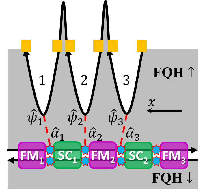
Figure 1: Schematic setup for a PF generalization of the topological Kondo effect. Two opposite-spin FQH edges (thick straight black arrows) are gapped out in different regions by the proximitizing FM and SC parts, where PF zero mode operators $\hat{\alpha}_{j}$ (blue stars) are localized at domain walls. (Strictly speaking, we have PF operators $\hat{\alpha}_{j}=\hat{\alpha}_{j,\uparrow}$ and $\hat{\alpha}_{j,\downarrow}$ at opposite-spin edges Snizhko2018 . Here only the $\hat{\alpha}_{j}$ are needed.) The $N=2$ SC domains are electrically connected to form a phase-coherent device with a common charging energy $E_{C}$. Similarly, FM domains belong to one bulk FM. The $M=3$ additional FQH edges (curved black arrows) serve as quasiparticle leads, where the quasiparticle operator $\hat{\psi}_{j}$ is tunnel-coupled (red dashed lines) to the respective PF operator $\hat{\alpha}_{j}$. Although different leads are parts of a single long edge, they must be dynamically independent. To that end, Ohmic contacts (yellow rectangles) are inserted between them.

As shown in Fig. 1, several additional FQH edges can now serve as probing leads in transport studies. Fractional quasiparticles in these edges are thereby tunnel-coupled to the PF operator $\hat{\alpha}_{j}$ at the respective domain wall. A general setup consists of a PF box made of $N$ SC domains and contacted by $3\leq M\leq 2N$ edge states. We show the simplest non-trivial case with $N=2$ and $M=3$ in Fig. 1. It is important that the PF box device is kept floating (not grounded) such that the total charge on the PF box is restricted by the Coulomb charging energy.

Let us first outline the theoretical description of the FQH edge state leads. Each of the $M$ lead pieces is described by a chiral boson field, $\hat{\phi}_{j}(x)$, with the Hamiltonian Wen1991 ; Kane1992a ; Gogolin1998 ; Altland2010

$$H_{\mathrm{edge}}=\sum_{j=1}^{M}\frac{v}{4\pi}\int_{-L/2}^{+L/2}dx(\partial_{x}\hat{\phi}_{j})^{2},$$ (2)

where $v$ is the edge velocity, assumed identical in all leads. Anisotropies in these velocities do not cause physical effects since they can be absorbed by a renormalization of cotunneling amplitudes. Since we are not interested in finite-size effects in the leads, we will also assume $L\to\infty$. The commutation relations between chiral boson fields,

$$[\hat{\phi}_{j}(x),\hat{\phi}_{k}(x^{\prime})]=i\pi\left[\delta_{jk}\mathrm{sgn}(x-x^{\prime})+\mathrm{sgn}(k-j)\right],$$ (3)

already incorporate Klein factors Gogolin1998 since Eq. (3) follows from a single-edge commutation relation by imagining that all leads actually belong to one long edge. It is important, however, that different leads are dynamically independent, which in turn is ensured by the Ohmic contacts in Fig. 1. The fractional quasiparticle operator can then be expressed as vertex operator of the respective chiral boson field, $\hat{\psi}_{j}(x)\sim\ e^{i\sqrt{\nu}\hat{\phi}_{j}(x)}$, see Refs. Wen1991 ; Kane1992a ; Gogolin1998 ; Altland2010 and App. A.

Next, we summarize the theoretical description of the PF box. For detailed derivations and discussions, see Refs. Lindner2012 ; Clarke2013 ; Snizhko2018 . The PF box is defined from opposite-spin FQH edges which are proximitized by alternating FM and SC domains, see Fig. 1. Since at low energy scales, these domains are gapped, operators creating low-energy excitations can only reside at the domain walls in between adjacent domains. Similar to the Majorana case, the domain wall hosts stable zero-energy modes corresponding to the PF operators $\hat{\alpha}_{j}$. The latter obey the $\mathbb{Z}_{n}$ PF algebra with index $n=2/\nu$,

$$\hat{\alpha}_{j}\hat{\alpha}_{k}=\omega^{\mathrm{sgn}(k-j)}\hat{\alpha}_{k}\hat{\alpha}_{j},\quad\omega=e^{2\pi i/n}=e^{i\pi\nu}.$$ (4)

The low-energy PF box Hilbert space is spanned by the states $|Q_{\mathrm{tot}},Q_{1}\mathrm{mod}\leavevmode\nobreak\ 2,...,Q_{N-1}\mathrm{mod}\leavevmode\nobreak\ 2\rangle$, where $Q_{{\rm tot}}$ is the total charge of the proximitizing SCs and the FQH edges within the PF box. Importantly, $Q_{{\rm tot}}$ has fractional values differing by multiples of $\nu$. We note that here all SC_j pieces are implied to be part of one floating superconductor, and similarly all FM_j are part of one ferromagnet. The quantum numbers $Q_{j}$ describe the charge of the FQH edges trapped between FM_j and FM_j+1, and are also quantized in units of $\nu$. Since the proximitizing SCs can absorb Cooper pairs at no kinetic energy cost, the $Q_{j}$ are only defined modulo 2. These quantum numbers correspond to the distribution of fractional quasiparticles between different SC_j parts. The box Hamiltonian only receives a Coulomb charging contribution sensitive to the total charge $Q_{{\rm tot}}$,

$$H_{\mathrm{box}}=E_{C}\left(\hat{Q}_{{\rm tot}}-q_{0}\right)^{2}.$$ (5)

By changing a backgate voltage, one can tune the parameter $q_{0}$ such that the box has quantized ground-state charge given by the value of $Q_{{\rm tot}}$ closest to $q_{0}$. For special choices of $q_{0}$, one may also reach charge degenerate points, but such cases are not considered here.

Finally, we include complex-valued tunneling amplitudes $\eta_{j}$ describing tunneling of quasiparticles between the respective edge ($\hat{\psi}_{j}$) through the FQH bulk to the PF box via $\hat{\alpha}_{j}$. Assuming a point-like tunnel contact at $x=0$ along the respective edge, the tunneling Hamiltonian is given by Lindner2012 ; Snizhko2018

$$H_{\mathrm{tun}}=\sum_{j=1}^{M}\eta_{j}\hat{\psi}_{j}(0)\hat{\alpha}_{j}^{\dagger}+\mathrm{h.c.}$$ (6)

Using Eq. (3), the fractional quasiparticle operators $\hat{\psi}_{j}(x)\sim e^{i\sqrt{\nu}\hat{\phi}_{j}(x)}$ obey the algebra

$$\hat{\psi}_{j}(x)\hat{\psi}_{k}(x^{\prime})=e^{-i\pi\nu\mathrm{sgn}(k-j)-i\pi\nu\delta_{jk}\mathrm{sgn}(x-x^{\prime})}\hat{\psi}_{k}(x^{\prime})\hat{\psi}_{j}(x).$$ (7)

Furthermore, one can show that $\left[\hat{\phi}_{j}(x),\hat{\alpha}_{k}\right]=-\pi\sqrt{\nu}$ holds. From the latter relation, we obtain

$$\hat{\psi}_{j}(x)\hat{\alpha}_{k}=e^{-i\pi\nu}\hat{\alpha}_{k}\hat{\psi}_{j}(x).$$ (8)

Altogether these relations imply that all terms in Eq. (6) commute with each other. This fact will become important when we discuss the strong-coupling regime in Sec. IV. We emphasize that Klein factors, which are needed to ensure proper statistical phase relations between different edges Gogolin1998 , are fully taken into account by Eqs. (3), (4), (7) and (8).

For a generic backgate parameter $q_{0}$ in Eq. (5), the ground state of the PF box has quantized charge $Q_{\mathrm{tot}}$ due to the large charging energy $E_{C}$. The dominant low-energy processes then come from the cotunneling of fractional quasiparticles between different edges mediated by the PF box. Technically, one obtains the cotunneling Hamiltonian, $H_{{\rm cot}}$, by projecting the full Hamiltonian, $H=H_{{\rm edge}}+H_{{\rm box}}+H_{{\rm tun}}$, to the charge ground-state sector of the PF box, $H\to H_{{\rm eff}}=H_{{\rm edge}}+H_{{\rm cot}}.$ A standard Schrieffer-Wolff transformation Altland2010 ; Schrieffer1966 yields

$$H_{\mathrm{cot}} = -\sum_{j,k=1;j\neq k}^{M}\lambda_{jk}\hat{\psi}_{j}^{\dagger}(0)\hat{\psi}_{k}(0)\hat{\alpha}_{j}\hat{\alpha}_{k}^{\dagger}$$

$$- \sum_{j}\left|\eta_{j}\right|^{2}\left(U_{+}^{-1}\hat{\psi}_{j}^{\dagger}(0)\hat{\psi}_{j}(0)+U_{-}^{-1}\hat{\psi}_{j}(0)\hat{\psi}_{j}^{\dagger}(0)\right),$$

where the cotunneling amplitude from lead $k$ to lead $j$ is

$$\lambda_{jk}=\eta_{j}^{*}\eta_{k}\left(U_{+}^{-1}+U_{-}^{-1}\right).$$ (10)

Here, $U_{+}$ ($U_{-})$ denotes the energy cost for adding (removing) one fractional quasiparticle to (from) the box. For instance, assuming $|q_{0}|<\nu/2$, one finds $U_{\pm}=E_{C}\nu^{2}(1\mp 2q_{0}/\nu)$. As shown in App. A, for $\nu\leq 1$, the potential scattering terms corresponding to the second row in Eq. (II) can always be neglected. In addition, the complex phases of $\eta_{j}$ can be gauged away by shifting the respective boson field, $\hat{\phi}_{j}(x)\to\hat{\phi}_{j}(x)+{\rm cst}$. This gauge transformation renders all $\lambda_{jk}$ in Eq. (10) real positive and symmetric, $\lambda_{kj}=\lambda_{jk}>0$. We note in passing that the total electric charge on the PF box is explicitly preserved by Eq. (II), as well as the total $\mathbb{Z}_{n}$ charge described in Ref. Alicea2016 . In addition, we remark that the original derivation by Schrieffer and Wolff contains a term beyond Eq. (II), see Eq. (12) in Ref. Schrieffer1966 . A similar term describing the simultaneous tunneling of two quasi-particles onto/off the impurity arises in our case. However, this term does not preserve the PF box electric charge and thus vanishes after the projection to the charge ground state.

Our PF generalization of the topological Kondo model thus corresponds to the effective low-energy Hamiltonian

$$H_{{\rm eff}}=\sum_{j=1}^{M}\frac{v}{4\pi}\int_{-\infty}^{\infty}dx(\partial_{x}\hat{\phi}_{j})^{2}-\sum_{j\neq k}^{M}\lambda_{jk}\hat{\psi}_{j}^{\dagger}(0)\hat{\psi}_{k}(0)\hat{\alpha}_{j}\hat{\alpha}_{k}^{\dagger},$$ (11)

together with the commutation relations in Eqs. (3), (4), (7), and (8).

At this point several remarks are in order.

[i)]

1. For $\nu=1$, noting that $\hat{\alpha}_{j}\hat{\alpha}_{k}^{\dagger}\to\gamma_{j}\gamma_{k}$, the quantum impurity spin operator in Eq. (11) has the components $i\gamma_{j}\gamma_{k}$. These Majorana bilinears generate the algebra so$(M)$ Beri2012 ; Zazunov2014 , and Eq. (11) reduces to the TKE Hamiltonian. For $M=3$, the three independent bilinears are equivalently expressed by standard Pauli operators, so$(3)=$ su$(2)$.

2. For $\nu<1$, the PF box also has a continuous symmetry. The PF bilinears $\hat{\alpha}_{j}\hat{\alpha}_{k}^{\dagger}$ appearing in Eq. (11) do not constitute a closed Lie algebra. However, together with their powers and products of those, they close the algebra su$\left(n^{[(M-1)/2]}\right)$, where $[x]$ is the integer part of $x$, acting onto the PF box Hilbert space in the fundamental representation footnote1 . In particular, for $M=3$, the algebra su$(n)$ is generated by the set of operators

   $$\left\{\hat{\alpha}_{1}^{k_{1}}\hat{\alpha}_{2}^{k_{2}}\hat{\alpha}_{3}^{-k_{1}-k_{2}}\right\},$$ (12)

   where integers $k_{j}$ are defined modulo $n=2/\nu$ as $\hat{\alpha}_{j}^{n}=1$, and we use the convention $\hat{\alpha}_{j}^{-k}\equiv(\hat{\alpha}_{j}^{\dagger})^{k}$ for $k>0$. The fact that the dimension of the ‘quantum impurity’ representation space is $n$ follows from the PF representation in Refs. Alicea2016 ; Dong2017 together with the $\mathbb{Z}_{n}$-charge conservation constraint. For $\nu=1/3,$ we arrive at su(6) with its 35 generators plus the identity, which are given by Eq. (12). Note that the bilinears $\hat{\alpha}_{j}\hat{\alpha}_{k}^{\dagger}$ appearing in the Hamiltonian (11) themselves constitute only a small subset of six out of the 35 algebra generators.

3. The leads, however, in general do not possess a continuous symmetry, cf. App. B. This situation should be contrasted to standard Kondo problems (including the TKE), where both the impurity and the leads constitute representations of a symmetry group, and the interaction between them is built out of currents generating this symmetry in each part.

4. Nonetheless, Eq. (11) shows that basic ingredients of a typical quantum impurity setting are present. A schematic sketch of $H_{{\rm eff}}$ in Eq. (11) is depicted in Fig. 2, where $M$ (parallel) chiral edges interact by cotunneling processes of fractional quasiparticles at $x=0$ between different lead pairs. Simultaneously, such exchange processes cause transitions in the PF box Hilbert space via the PF bilinears $\sim\hat{\alpha}_{j}\hat{\alpha}_{k}^{\dagger}$.

Figure 2: Schematic view of the effective Hamiltonian $H_{{\rm eff}}$ in Eq. (11), which defines a PF generalization of the topological Kondo model. Here, $M=3$ fractional edge state leads are connected via pairwise cotunneling processes at $x=0$. Each cotunneling event comes with a transition in the PF Hilbert space (indicated by the vertical colored bar).

III RG analysis

We now turn to the weak-coupling regime and discuss the one-loop RG equations for the PF generalization of the topological Kondo model in Eq. (11). To that end, consider a perturbative expansion of the partition sum in powers of the cotunneling amplitudes $\lambda_{jk}=\lambda_{kj}>0$. Within the RG approach Altland2010 , upon reducing the effective bandwidth $\Lambda$ from its bare value, $\Lambda(\ell=0)\approx E_{C}$, one analyzes how these couplings are renormalized and whether new types of couplings will be generated. Writing $\Lambda(\ell)=\Lambda(0)e^{-\ell}$, the scale $\Lambda(\ell)$ refers to the energy scale at which the system is probed with increasing RG flow parameter $\ell$. In case the RG flow of the $\lambda_{jk}(\ell)$ approaches the strong-coupling limit, the RG approach breaks down at $\ell=\ell^{*}$ where one hits a divergence of the dominant coupling. The corresponding scale defines the Kondo temperature,

$$T_{K}=\Lambda(\ell^{*})=E_{C}e^{-\ell^{*}}.$$ (13)

The physics in the strong-coupling regime, i.e., for energies well below $T_{K}$, will be addressed in Sec. IV.

The one-loop RG equations are most conveniently obtained via the operator product expansion (OPE) approach Cardy1996 , where one considers arbitrary pairs of cotunneling operators in Eq. (11) at almost coinciding times $t$ and $t^{\prime}$. The result of such a contraction must be equivalent to a linear combination of all possible boundary operators taken at time $(t+t^{\prime})/2$, and the expansion coefficients directly determine the one-loop RG equations Cardy1996 . One thus has to analyze contractions of cotunneling operators, cf. App. A. Most contractions imply a renormalization of a cotunneling amplitude $\lambda_{jk}$. However, one also finds additional contributions generating new couplings. For instance, a contraction of the cotunneling operators corresponding to $\lambda_{kj}$ and $\lambda_{km}$ (with $k\neq j\neq m$) generates a coupling to the operator

$$H^{\prime}=\left(\hat{\psi}_{k}^{\dagger}(0)\right)^{2}\hat{\psi}_{j}(0)\hat{\psi}_{m}(0)\hat{\alpha}_{k}^{2}\hat{\alpha}_{j}^{\dagger}\hat{\alpha}_{m}^{\dagger},$$ (14)

which has scaling dimension $\Delta^{\prime}=3\nu$. Since the cotunneling terms $\sim\lambda_{jk}$ in Eq. (11) have the smaller scaling dimension $\Delta_{jk}=\nu$, we conclude that $H^{\prime}$ is much less relevant (in fact marginal for $\nu=1/3$, and irrelevant for $\nu=2/3$) and thus can be dropped. Contractions of cotunneling operators then only produce PF bilinears of the type $\sim\hat{\alpha}_{j}\hat{\alpha}_{k}^{\dagger}$ already present in Eq. (11). In particular, for $M=3$, all other impurity operators in the set (12) are not activated.

Remarkably, after a uniform rescaling,

$$\tilde{\lambda}_{jk}=\frac{2\tau_{c}^{1-\nu}}{v^{\nu}}\lambda_{jk},$$ (15)

where $\tau_{c}$ denotes a short-time cutoff, we find that the RG equations for our PF generalization coincide with those for the Majorana-based TKE with Luttinger liquid parameter $g=1/\nu$ Altland2013 ; Beri2013 ,

$$\frac{d\tilde{\lambda}_{jk}}{d\ell}=(1-\nu)\tilde{\lambda}_{jk}+\sum_{m\neq(j\neq k)}^{M}\tilde{\lambda}_{jm}\tilde{\lambda}_{mk}.$$ (16)

Consider first the isotropic part of the cotunneling couplings. Writing $\tilde{\lambda}_{jk}=\tilde{\lambda}(1-\delta_{jk})$, Eq. (16) yields

$$\frac{d\tilde{\lambda}}{d\ell}=(1-\nu)\tilde{\lambda}+(M-2)\tilde{\lambda}^{2},$$ (17)

which is solved by

$$\tilde{\lambda}(\ell)=\frac{\tilde{\lambda}(0)e^{(1-\nu)\ell}}{1+\frac{M-2}{1-\nu}\tilde{\lambda}(0)[1-e^{(1-\nu)\ell}]}.$$ (18)

Clearly, the isotropic part $\tilde{\lambda}(\ell)$ flows towards strong coupling and diverges once the running energy scale reaches the Kondo temperature in Eq. (13). We find

$$T_{K}\simeq E_{C}\left(\frac{(M-2)\tilde{\lambda}(0)}{1-\nu}\right)^{1/(1-\nu)}.$$ (19)

The power-law dependence of $T_{K}$ on the average cotunneling coupling $\tilde{\lambda}(0)$ should be contrasted to the $T_{K}\sim e^{-1/[(M-2)\tilde{\lambda}(0)]}$ law of the TKE for $\nu=1$ Beri2012 . Equation (19) thus suggests that much higher $T_{K}$ are possible for $\nu<1$. We note that although the notation $T_{K}$ is suggestive of a ‘Kondo temperature’, Eq. (19) only indicates the separation between the regimes of strong and weak coupling. Indeed, as discussed above, for $\nu<1$, the leads do not possess a continuous symmetry, and hence one cannot speak of Kondo screening processes in the usual sense. Finally, in order to show that anisotropies in the cotunneling amplitudes are negligible as in the conventional TKE Beri2012 , we have linearized the RG equations (16) in the $\tilde{\lambda}_{jk}$ anisotropies taken relative to the isotropic component. Our analysis shows that relative anisotropies are RG irrelevant and thus can be neglected at low energy scales.

IV Strong-coupling solution

We next turn to the strong-coupling regime realized at energy scales well below $T_{K}$ in Eq. (19). We here pursue a similar strategy as done for the TKE in Refs. Altland2013 ; Beri2013 ; Zazunov2014 . To that end, we take the bosonized version of Eq. (11), with $\hat{\psi}_{j}(0)\sim e^{i\sqrt{\nu}\hat{\phi}_{j}(0)}$, and consider the limit $\lambda_{jk}\to+\infty$. As a result, in the ground state of the system, the phase fields $\hat{\phi}_{j}(0)$ will be locked into a configuration minimizing the cosine potentials resulting from $H_{{\rm cot}}$. Using the general approach of Ref. Ganeshan2016 , one can then construct the low-energy Hamiltonian describing this fixed point. We also systematically compute all possible operator perturbations around the fixed point and thereby show that it is stable. The leading irrelevant operators then determine the finite-$T$ corrections to the conductance tensor, where we will compare our results to the TKE expression in Eq. (1).

IV.1 Strong-coupling fixed point

Using Eqs. (4), (7) and (8), one finds that all cotunneling operators $\hat{\psi}_{j}^{\dagger}(0)\hat{\psi}_{k}(0)\hat{\alpha}_{j}\hat{\alpha}_{k}^{\dagger}$ in Eq. (11) are mutually commuting and thus can be diagonalized simultaneously. At the putative strong-coupling fixed point, we now demand that each of those terms is separately minimized. Defining auxiliary operators $\hat{\beta}_{jk}$,

$$\hat{\alpha}_{j}\hat{\alpha}_{k}^{\dagger}=e^{i\pi\hat{\beta}_{jk}-i\pi\nu\mathrm{sgn}(k-j)},$$ (20)

Equation (11) yields

$$H_{{\rm cot}}=-\frac{2}{(v\tau_{c})^{\nu}}\sum_{j>k}\lambda_{jk}\cos\left(\sqrt{\nu}\left[\hat{\phi}_{k}(0)-\hat{\phi}_{j}(0)\right]+\pi\hat{\beta}_{jk}\right).$$ (21)

Minimizing $H_{{\rm cot}}$ for $\lambda_{jk}\to+\infty$ is then equivalent to imposing the constraints

$$\sqrt{\nu}\left[\hat{\phi}_{k}(0)-\hat{\phi}_{j}(0)\right]+\pi\hat{\beta}_{jk}=2\pi\hat{C}_{jk},$$ (22)

where $\hat{C}_{jk}$ are integer-valued operators. We note that the commutation relations $[\hat{\beta}_{jk},\hat{\phi}_{m}(x)]=0$ and

$$[\hat{\beta}_{jk},\hat{\beta}_{mn}] = i\frac{\nu}{\pi}\Bigl{[}\mathrm{sgn}(j-m)+\mathrm{sgn}(k-n)$$ (23)

$$- \mathrm{sgn}(j-n)-\mathrm{sgn}(k-m)\Bigr{]}$$

imply that $[\hat{C}_{jk},\hat{C}_{mn}]=0.$ In addition, with $\hat{\beta}_{jk}+\hat{\beta}_{km}=\hat{\beta}_{jm}$, we see that $\hat{C}_{jk}+\hat{C}_{km}=\hat{C}_{jm}$. As a consequence, to enforce that all $\hat{C}_{jk}$ are integer, it suffices to demand that all $\hat{C}_{1j}$ with $j=2,\ldots,M$ are integer-valued operators.

For constructing the low-energy theory, we next employ the powerful approach of Ref. Ganeshan2016 , which is tailor-made to solving problems with large-amplitude cosine potentials as encountered here. According to this method, the $\hat{C}_{jk}$ should be constrained to being integer numbers, where the low-energy Hamiltonian $H_{\mathrm{LE}}$ follows from the free part, $H_{0}=H_{\mathrm{edge}}$ in Eq. (2), minus all terms causing a non-trivial time evolution of the $\hat{C}_{jk}$ in Eq. (22). The resulting Hamiltonian is quadratic and can easily be quantized. Delegating technical details to App. C, the quantized phase fields $\hat{\phi}_{j}(x,t)$ are expressed in terms of standard boson operators $\hat{a}_{q,j}$ (zero-mode operators $\hat{\phi}_{0,j}$) for each $\omega\neq 0$ ($\omega=0$) eigenfunction, cf. Eq. (A) in App. A. To that end, we define the matrix

$$U_{jk}=\frac{2}{M}-\delta_{jk},$$ (24)

and the operators

$$\hat{f}_{j}(x,t) = \hat{\phi}_{0,j}+\hat{g}_{j}(x,t),$$

$$\hat{g}_{j}(x,t) = i\int_{0}^{\infty}\frac{dq}{\sqrt{q}}\left(\hat{a}_{q,j}e^{iq(x-vt)}-{\rm h.c.}\right),$$ (25)

with the commutation relations

$$\left[\hat{a}_{q,j},\hat{a}_{q^{\prime},m}^{\dagger}\right]=\delta(q-q^{\prime})\delta_{jm},\quad\left[\hat{a}_{q,j},\hat{a}_{q^{\prime},m}\right]=0,$$ (26)

and $\left[\hat{\phi}_{0,j},\hat{\phi}_{0,m}\right]=i\pi\mathrm{sgn}(m-j)$. For incoming states ($x<0$), the chiral boson field is

$$\hat{\phi}_{j}(x<0,t)=\hat{f}_{j}(x,t),$$ (27)

while outgoing states ($x>0$) are given by

$$\hat{\phi}_{j}(x>0,t) = \sum_{k=1}^{M}U_{jk}\hat{f}_{k}(x,t)+$$

$$+ \frac{2\pi}{M}\sqrt{\nu^{-1}}\sum_{k=1,k\neq j}^{M}\left(\hat{\beta}_{jk}-2\hat{C}_{jk}\right).$$

The field at $x=0$ follows from the above relations, $\hat{\phi}_{j}(0,t)=[\hat{\phi}_{j}(0^{+},t)+\hat{\phi}_{j}(0^{-},t)]/2$, and the low-energy Hamiltonian $H_{{\rm LE}}$ takes the form, cf. Eq. (63) in App. C,

$$H_{\mathrm{LE}}=\sum_{j=1}^{M}\int_{0}^{\infty}dq\ vq\left(\hat{a}_{q,j}^{\dagger}\hat{a}_{q,j}+\frac{1}{2}\right).$$ (29)

For a discussion of transport features, we next note that the current flowing along an edge corresponds to the operator Wen1991 ; Kane1992a ; Gogolin1998 ; Altland2010

$$\hat{I}_{j}(x,t)=-\frac{\sqrt{\nu}}{2\pi}\partial_{t}\hat{\phi}_{j}(x,t).$$ (30)

Using Eqs. (24)–(IV.1), we find

$$\hat{I}_{j}(x,t)=-\frac{\sqrt{\nu}}{2\pi}\sum_{k}\left[\theta(x)U_{jk}+\theta(-x)\delta_{jk}\right]\partial_{t}\hat{g}_{k}(x,t),$$ (31)

with the Heaviside function $\theta(x)$. We thus observe that

$$\hat{I}_{j}(0^{+},t)=\sum_{k=1}^{M}U_{jk}\hat{I}_{k}(0^{-},t).$$ (32)

At low frequencies $\omega=vq\to 0$, we obtain

$$I_{j}^{+}=\sum_{k}U_{jk}I_{k}^{-}=\nu\frac{e^{2}}{h}\sum_{k}U_{jk}V_{k},$$ (33)

where $I_{j}^{+/-}=\left\langle\hat{I}_{j}(x>0/x<0,t)\right\rangle$ refers to the scattered/incoming current, respectively. The incoming current is given by $I_{j}^{-}=\nu e^{2}V_{j}/h$, where $V_{j}$ is the voltage for injected quasiparticles at the $j$th edge.

At the strong-coupling fixed point ($T=V_{j}=0$), we thus obtain the universal multi-terminal conductance tensor

$$G_{jk}=\frac{dI_{j}^{+}}{dV_{k}}=\frac{\nu e^{2}}{h}U_{jk}=\frac{\nu e^{2}}{h}\left(\frac{2}{M}-\delta_{jk}\right).$$ (34)

For $\nu=1$, taking into account that the injection and collection points are spatially separated in our Hall setup, Eq. (34) has the same physical content as the $T=0$ TKE conductance in Eq. (1). Indeed, Eq. (34) describes the scattered current $I_{j}^{+}$. Studying instead the current at the tunnel contact, $I_{j}=I_{j}^{+}-I_{j}^{-}$, we have to replace $U_{jk}\to U_{jk}-\delta_{jk}=2\left(\frac{1}{M}-\delta_{jk}\right)$ in Eq. (34). After this step, Eq. (34) matches the TKE conductance tensor in Eq. (1) taken at $T=0$. Remarkably, the isotropic structure of the TKE conductance (1) carries over to the $\nu<1$ PF generalization, despite of the fact that we are not dealing with a Kondo problem anymore.

A particularly noteworthy consequence of Eq. (34) is revealed by inspecting the diagonal component of the conductance tensor, which has the universal, fractionally quantized, and negative value

$$G_{jj}=-\frac{M-2}{M}\frac{\nu e^{2}}{h}<0.$$ (35)

Since this conductance is negative, our device can be operated as current extractor. For instance, putting all $V_{k}=0$ except for $V_{1}\neq 0$, current is injected only via the first lead, $I_{1}^{-}=\frac{\nu e^{2}}{h}V_{1}\equiv I_{{\rm in}}$. The outgoing current in this lead then has the opposite sign, $I_{1}^{+}=-\frac{M-2}{M}I_{{\rm in}}<0$, where the fraction $-I_{1}^{+}/I_{{\rm in}}$ is determined only by the number $M$ of leads. For this example, the outgoing currents in all other $M-1$ leads ($j>1$) are identical and given by $I_{j}^{+}=\frac{2}{M}I_{{\rm in}}$, see Eq. (34). Current conservation, $I_{{\rm out}}=(M-1)I_{j}^{+}+I_{1}^{+}=I_{{\rm in}}$, thus requires that current must be extracted from lead $j=1$. Similar current extraction phenomena in quantum Hall devices have been discussed in Ref. Protopopov2017 .

Another striking consequence of Eq. (34) is the absence of current-current correlations between different terminals at the fixed point, which can be established from the above theory along the lines of Refs. Beri2013 ; Zazunov2014 . The absence of shot noise is noteworthy since incoming currents are partitioned into currents flowing through all leads attached to the PF box, see Eq. (34), and such partitioning processes usually generate noise Altland2010 . Noiseless partitioning of currents in multi-terminal quantum junctions has also been established for the TKE Beri2013 ; Zazunov2014 and for the related case of quantum Hall junctions coupled through a central quantum dot Altland2012 ; Altland2015 . In our system, leading irrelevant operators, see Sec. IV.2, can be responsible for weak contributions to shot noise. However, such contributions quickly vanish as one approaches the fixed point for $T,V_{j}\to 0$.

IV.2 Stability of the strong-coupling point

The stability of the strong-coupling fixed point and the low-energy physics in its vicinity are determined by the leading irrelevant operators (LIOs), where we anticipate that our analysis finds no marginal or relevant operators perturbing the fixed point. Such perturbations will appear because the $\lambda_{jk}$ couplings are large but finite and are constructed from admissible operators at the fixed point. The latter have to obey three requirements, namely (i) they do not change the charge $Q_{\mathrm{tot}}$ of the PF box, (ii) they change the total charge of each edge only in multiples of $\nu$, and (iii) they alter $\hat{C}_{jk}$ in Eq. (22) only by an integer number. Condition (i) prohibits operators with an odd number of PF operators $\hat{\alpha}_{m}^{\thinspace},\hat{\alpha}_{m}^{\dagger}$. Condition (ii) implies that operators $e^{\pm i\sqrt{\nu}\hat{\phi}_{j}(x,t)}$ (or multiples thereof) are involved. Finally, condition (iii) further constrains the set of allowed operators. By using (iii) in conjunction with the commutation relations

$$\left[\hat{C}_{jk}(t),e^{\pm i\sqrt{\nu}\hat{\phi}_{m}(x,t)}\right]=\pm\frac{\nu}{2}\Bigl{(}\mathrm{sgn}(x)\left(\delta_{km}-\delta_{jm}\right)\\ +\mathrm{sgn}(k-m)-\mathrm{sgn}(j-m)\Bigr{)}e^{\pm i\sqrt{\nu}\hat{\phi}_{m}(x,t)}$$ (36)

and $\left[\hat{C}_{jk}(t),e^{i\sqrt{\nu}\hat{\phi}_{m}(0,t)}\hat{\alpha}_{m}^{\dagger}\right]=0$, one can determine all admitted operators at the strong-coupling fixed point. The list of elementary allowed operators is given in Table 1. All non-trivial allowed operators can be constructed by taking composites of the operators in Table 1. Note that the list implies that electrons can tunnel in and out of the system anywhere at $x\neq 0$, but quasiparticles can only tunnel outside of the whole structure or between neighboring edges. Since quasiparticles have to tunnel through the FQH bulk, these are also the only physical possibilities in Fig. 1.

$\hat{O}$	$\Delta_{\hat{O}}$
$e^{\pm i\sqrt{\nu}\hat{\phi}_{1}(x>0,t)}$	$\nu/2$
$e^{\pm i\sqrt{\nu}\hat{\phi}_{M}(x<0,t)}$	$\nu/2$
$e^{\pm i\sqrt{\nu}\left(\hat{\phi}_{j}(x>0,t)-\hat{\phi}_{j-1}(x^{\prime}<0,t)\right)}$	$\nu\left(1-\frac{2}{M}\right)$, when $x=-x^{\prime}=0^{+}$
$e^{\pm i\sqrt{\nu^{-1}}\hat{\phi}_{j}(x\neq 0,t)}$	$\nu^{-1}/2$

Table 1: Elementary allowed operators $\hat{O}$ and their scaling dimensions $\Delta_{\hat{O}}$ at the strong-coupling fixed point. Combinations of them lead to non-trivial new scaling dimensions.

The scaling dimensions of operators and their combinations are easily obtained by expressing operators in terms of $\hat{g}_{j}(x,t)$, see Eq. (25), and ignoring zero modes. Indeed, the operator $e^{i\sum_{j}p_{j}\hat{g}_{j}(x,t)}$ is seen to have scaling dimension $\Delta=\sum_{j}p_{j}^{2}/2$ by means of the relation

$$\left\langle e^{i\sum_{j}p_{j}\hat{g}_{j}(x,t)}e^{-i\sum_{j}p_{j}\hat{g}_{j}(x,t^{\prime})}\right\rangle\sim(t-t^{\prime}-i0^{+})^{-\sum_{j}p_{j}^{2}}.$$ (37)

Next we calculate the scaling dimension of the LIO. Within the original Hamiltonian (11), transfer of charge between different edges is only possible through exponentials of $\hat{C}_{jk}$. A non-trivial perturbation to the strong-coupling fixed point can then only result from edge fields $\hat{\phi}_{m}(x,t)$ taken near $x=0$ on a single edge $m$. The most general perturbation has the form

$$\hat{O}_{c}\sim e^{i\sqrt{\nu^{-1}}\left(d_{+}\hat{\phi}_{m}(0^{+},t)+d_{-}\hat{\phi}_{m}(0^{-},t)\right)},\quad d_{\pm}\in\mathbb{Z}.$$ (38)

Since this operator should conserve total charge, we require $d_{-}=-d_{+}$. Then $\hat{O}_{c}$ shifts $\hat{C}_{jk}\rightarrow\hat{C}_{jk}+d_{+}\left(\delta_{km}-\delta_{jm}\right)$, while its scaling dimension is given by $\Delta_{c}=d_{+}^{2}\frac{2}{\nu}\left(1-\frac{1}{M}\right)$. The LIO follows for $d_{+}=\pm 1$ (where $\hat{O}_{c}$ coincides with $e^{\mp i\hat{\Pi}_{m}}$ in App. C), with the scaling dimension

$$\Delta_{\mathrm{LIO}}=\frac{2}{\nu}\left(1-\frac{1}{M}\right).$$ (39)

For all $M\geq 3$ and $\nu\leq 1$, we observe that $\Delta_{\mathrm{LIO}}>1$. The fixed point is thus stable as asserted before. Furthermore, since $\Delta_{\mathrm{LIO}}=\Delta_{M}$ in Eq. (1), with Luttinger liquid parameter $g=\nu^{-1}$, the finite-$T$ corrections at $T\ll T_{K}$ for the linear conductance tensor can be inferred from Eq. (1) as well,

$$G_{jk}=\frac{dI_{j}^{+}}{dV_{k}}=\nu\frac{e^{2}}{h}\left[1-(T/T_{K})^{2\Delta_{\mathrm{LIO}}-2}\right]\left(\frac{2}{M}-\delta_{jk}\right).$$ (40)

Transport features are therefore basically identical to the Majorana-based TKE, and also the PF-based strong-coupling point represents a local quantum-critical point of non-Fermi-liquid type.

We close this section with two remarks. First, consider operators of the form $e^{\pm i\sqrt{\nu}\left(\hat{\phi}_{j}(x>0,t)-\hat{\phi}_{j-1}(x^{\prime}<0,t)\right)}$. Such operators do not appear as perturbations within the Hamiltonian in Eq. (11), which contains no direct tunneling processes between different edges. In general, such couplings can appear and destabilize the fixed point, even though these operators do not induce transitions between different values of $\hat{C}_{jk}$, i.e., between different ground-state minima of the potential in Eq. (21). Indeed, they couple the incoming and outgoing channels in the scattering problem. Should the corresponding coupling strength be non-vanishing, it will destabilize the fixed point below some energy scale. In practice, these couplings (and the associated destabilization energy scale) can be suppressed by arranging the respective edge parts far away from each other.

Second, it is also instructive to consider operators $\hat{O}\sim e^{i\sqrt{\nu}\hat{\phi}_{m}(0)}\hat{\alpha}_{m}^{\dagger}$, which commute with $\hat{C}{}_{jk}$ and have scaling dimension $\Delta=\nu/(2M)$, with $\Delta<\nu/2$ for $M\geq 2$. Therefore, if several couplings $\lambda_{jk}$ in Eq. (11) enter the strong-coupling regime and approach a fixed point with $M^{\prime}<M$ leads, the couplings to the remaining leads will quickly catch up under the RG flow since they are relevant. In fact, they are even more relevant than the original couplings in Eq. (11).

V Conclusions

In this work, we have proposed a parafermionic version of the topological Kondo model previously suggested for a Majorana box Beri2012 ; Altland2013 ; Beri2013 . Our generalization employs chiral fractional quantum Hall edge states as leads, which are tunnel-coupled to parafermionic zero modes present on a Coulomb-blockaded island, cf. Ref. Snizhko2018 . By means of Abelian bosonization, a theoretical description of quantum transport in such a multi-terminal quantum junction has been given in both the weak- and the strong-coupling limit. In particular, we have derived and discussed the one-loop RG equations. Our RG analysis shows that the system flows towards an isotropic stable strong-coupling fixed point. However, in contrast to the Majorana-based case, our problem does not fall into the class of Kondo problems, see App. B for details.

The strong-coupling limit has then been analyzed by means of the approach of Ref. Ganeshan2016 , which yields controlled results within the Abelian bosonization approach. It is remarkable that the resulting conductance tensor is basically identical to the one of the Majorana-based topological Kondo model, see Eq. (1), even though no continuous symmetries (and hence no Kondo screening processes) are manifestly involved in the PF variant. Let us emphasize two particularly noteworthy features of our $T=0$ result in Eq. (34). First, the isotropic partitioning of injected quasiparticle currents into all outgoing leads is noiseless, in analogy to previous studies for different but related physical systems Beri2012 ; Altland2013 ; Beri2013 ; Zazunov2014 ; Altland2012 ; Altland2015 . Second, consider the case that a current $I_{{\rm in}}$ is injected only via lead 1. This lead then also serves as current extractor, since the outgoing current $I_{1}^{+}$ has opposite sign as compared to the injected current, with the universal ratio $I_{1}^{+}/I_{{\rm in}}=-(M-2)/M$. By determining the leading irrelevant operators around the strong-coupling point, we have also obtained the temperature-dependent corrections to the conductance tensor and established that the strong-coupling point represents a local quantum-critical point of non-Fermi liquid type. Given the recent experimental advances in the field Ronen2018 ; Wu2018 , we hope that these predictions can soon be put to an experimental test.

Appendix A On vertex operators

We here provide technical details related to Secs. II and III. We start by noting that in terms of the chiral boson fields in Eqs. (2) and (3), the fractional quasiparticle operator for the $j$th lead is given by $\hat{\psi}_{j}(x,t)=V_{\sqrt{\nu},j}(x,t)$, with the vertex operator

$$V_{p,j}(x,t)=\left(\frac{L}{2\pi}\right)^{-p^{2}/2}:e^{ip\hat{\phi}_{j}(x,t)}:,$$ (41)

where $:\ :$ denotes normal ordering and $L$ the system size. Using $\tau_{c}$ as short-time cutoff and a set of conventional boson operators $\{\hat{a}_{n,j}\}$ with momentum $k_{n}=2\pi n/L$ ($n\in\mathbb{N}$), $\hat{\phi}_{j}$ has the mode decomposition Gogolin1998

$$\hat{\phi}_{j}(x,t) = \hat{\phi}_{0,j}+\hat{Q}_{j}^{\mathrm{edge}}\frac{2\pi\left(x-vt\right)}{L\sqrt{\nu}}+i\sum_{n=1}^{\infty}\sqrt{\frac{2\pi}{Lk_{n}}}$$

$$\times \left(\hat{a}_{n,j}e^{ik_{n}(x-vt)}-\hat{a}_{n,j}^{\dagger}e^{-ik_{n}(x-vt)}\right)e^{-\tau_{c}vk_{n}/2},$$

where

$$\left[\hat{Q}_{j}^{\mathrm{edge}},\hat{\phi}_{0,m}\right]=i\sqrt{\nu}\delta_{jm},\quad\left[\hat{\phi}_{0,j},\hat{\phi}_{0,m}\right]=i\pi\mathrm{sgn}(m-j).$$ (43)

The operator $V_{p,j}$ in Eq. (41) has scaling dimension $\Delta_{p}=p^{2}/2$. The OPE contractions required for deriving the RG equations in Sec. III follow from the relation (with $x^{\prime}\to x$ and $t^{\prime}\to t$)

$$V_{p,j}(x,t)V_{q,j}(x^{\prime},t^{\prime})=\left(\frac{L}{2\pi}\right)^{-(p+q)^{2}/2}$$

$$\times\left[i(vt-x-vt^{\prime}+x^{\prime}-iv\tau_{c})\right]^{pq}\ :e^{i(p\hat{\phi}_{j}(x,t)+q\hat{\phi}_{j}(x^{\prime},t^{\prime}))}:$$

$$=\left[i(vt-x-vt^{\prime}+x^{\prime}-iv\tau_{c})\right]^{pq}$$

$$\quad\times\ V_{p+q,j}(x,t)\left[1+{\cal O}(x-x^{\prime})+{\cal O}(t-t^{\prime})\right].$$ (44)

Note that $pq=\Delta_{p+q}-\Delta_{p}-\Delta_{q}$.

Using Eq. (44) for $p=-q=\sqrt{\nu}$, and a regularization with positive infinitesimal $\varepsilon$, we can also verify that the potential scattering terms in Eq. (II) can be neglected. To that end, we write

$$\hat{\psi}_{j}(0)\hat{\psi}_{j}^{\dagger}(0) = \frac{1}{4\varepsilon^{2}}\int_{-\varepsilon}^{\varepsilon}dx\int_{-\varepsilon}^{\varepsilon}dx^{\prime}\ \hat{\psi}_{j}(x)\hat{\psi}_{j}^{\dagger}(x^{\prime})$$

$$= c_{0}+c_{1}\partial_{x}\hat{\phi}_{j}(0)+{\cal O}(c_{2}),\quad c_{m}\sim\varepsilon^{m-\nu}.$$

Now $c_{0}$ contributes only an unimportant (albeit divergent) constant while, for $\nu<1$, all $c_{m\geq 1}\to 0$ for $\varepsilon\to 0$. For $\nu=1$, $c_{1}$ remains finite for $\varepsilon\to 0$, but the corresponding term in Eq. (A) can be absorbed by the transformation $\hat{\phi}_{j}(x)\to\hat{\phi}_{j}(x)+\tilde{c}_{j}\mathrm{sgn}(x)$ with $\tilde{c}_{j}\sim c_{1}$. Since similar statements hold for $\hat{\psi}_{j}^{\dagger}(0)\hat{\psi}_{j}(0)$, we conclude that for all $\nu\leq 1$, potential scattering is indeed negligible.

Appendix B The (absent) symmetry of the leads

B.0.1 Lead symmetries

Kondo problems are characterized by coupling a set of leads, forming a representation of a continuous symmetry, with a quantum impurity sharing the same continuous symmetry. We here show that for our PF generalization of the TKE with $\nu<1$, the leads do not possess a non-trivial continuous symmetry. As a consequence, the corresponding model does not define a Kondo problem.

First of all, we note that for any $\nu\leq 1$ and any number $M$ of leads, we have a $[U(1)]^{M}$ symmetry related to charge conservation in each separate lead generated by the charge density operator $\frac{\sqrt{\nu}}{2\pi}\partial_{x}\hat{\phi}_{j}(x)$. This is not the symmetry we are interested in, as it is Abelian. All irreducible representations of an Abelian symmetry are necessarily one-dimensional, and, therefore, generators of such a symmetry cannot cause transitions of quasiparticles between the leads and the accompanying changes in the impurity state. Hence we are looking for non-Abelian symmetries of the leads, which should conserve total electric charge and the scaling dimensions of transformed operators. A fractional quasiparticle operator can thus only be transformed into a linear combination of such operators,

$$\hat{\psi}_{j}(x)\rightarrow\hat{\tilde{\psi}}_{j}(x)=\sum_{k}A_{jk}(x)\hat{\psi}_{k}(x).$$ (46)

The symmetry should preserve the quasiparticle permutation relations (7), which implies the conditions

$$\left(1-e^{i\pi\nu(\mathrm{sgn}(j-k)+\mathrm{sgn}(n-m))}e^{i\pi\nu\mathrm{sgn}(x-x^{\prime})(\delta_{mn}-\delta_{jk})}\right)$$

$$\quad\times A_{jm}(x)A_{kn}(x^{\prime})=0$$ (47)

for arbitrary $(j,k,m,n$) indices and arbitrary $x\neq x^{\prime}$. For a continuous symmetry, we focus on infinitesimal transformations, $A_{jk}(x)=\delta_{jk}+a_{jk}(x)$ with $|a_{jk}(x)|\ll 1$, where Eq. (47) yields (to linear order in $a_{jk}$ and putting $k=n$ and $j\neq m$)

$$\left(1-e^{i\pi\nu(\mathrm{sgn}(j-k)+\mathrm{sgn}(k-m))}e^{i\pi\nu\mathrm{sgn}(x-x^{\prime})(\delta_{mk}-\delta_{jk})}\right)\\ \times a_{jm}(x)=0.$$ (48)

Here $x^{\prime}$ remains as free parameter. Since the equation has to be satisfied both at $x^{\prime}>x$ and $x^{\prime}<x$, one concludes that either $\nu=1$ or $a_{jm}(x)=0$. For $\nu\neq 1$, this implies diagonal $A_{jm}(x)$ with Abelian symmetry, not mixing different edges. The above reasoning thus constitutes a proof that no continuous non-Abelian lead symmetry exists for $\nu\neq 1$.

B.0.2 Remarks on conformal field theory

$\nu$	$\Delta_{n}$
$1$	$0,\frac{1}{3},1,\frac{4}{3},\frac{7}{3},3,...$
$1/3$	$0,\frac{1}{9},\frac{1}{3},\frac{4}{9},\frac{7}{9},1,\frac{4}{3},\frac{13}{9},\frac{16}{9},\frac{19}{9},\frac{7}{3},\frac{25}{9},3,...$
$1/5$	$0,\frac{1}{15},\frac{1}{5},\frac{4}{15},\frac{7}{15},\frac{3}{5},\frac{4}{5},\frac{13}{15},\frac{16}{15},\frac{19}{15},\frac{7}{5},\frac{5}{3},\frac{9}{5},\frac{28}{15},\frac{31}{15},\frac{12}{5},...$

Table 2: The list of smallest neutral scaling dimensions of primary operators for $M=3$ leads at $\nu=1,\>1/3,\>1/5$.

It is instructive to study this issue also from the conformal field theory (CFT) Francesco1997 point of view. The leads are described by a CFT for massless chiral bosons. According to Noether’s theorem, a continuous symmetry implies the existence of a conserved current $J(x)$ generating the symmetry. In a chiral CFT, such currents must have scaling dimension $\Delta=1$, since the total charge associated with the conserved current, $\int dxJ(x)$, should not renormalize under scaling. Therefore, if a continuous lead symmetry is present, it must be generated by fields of scaling dimension $\Delta=1$. We now separate $H_{{\rm edge}}$ into a charged and a neutral sector. The charged sector is defined by the free boson field $\hat{\phi}_{c}(x)=\frac{1}{\sqrt{M}}\sum_{j=1}^{M}\hat{\phi}_{j}(x),$ with $\left[\hat{\phi}_{c}(x),\hat{\phi}_{c}(x^{\prime})\right]=i\pi\mathrm{sgn}(x-x^{\prime}).$ The total charge density, expressed through

$$\hat{\rho}_{c}(x)=\frac{\sqrt{\nu}}{2\pi}\partial_{x}\sum_{j=1}^{M}\hat{\phi}_{j}(x)=\frac{\sqrt{\nu M}}{2\pi}\partial_{x}\hat{\phi}_{c}(x),$$ (49)

generates the $U(1)_{c}$ symmetry responsible for total charge conservation. Writing $H_{\mathrm{edge}}=H_{c}+H_{n}$ with $H_{c}=\frac{v}{4\pi}\int_{-L/2}^{+L/2}dx\left(\partial_{x}\hat{\phi}_{c}(x)\right)^{2}$ and

$$H_{n}=\frac{v}{4\pi}\sum_{j=1}^{M}\int_{-L/2}^{+L/2}dx\left(\partial_{x}\hat{\phi}_{j}(x)-\frac{1}{\sqrt{M}}\partial_{x}\hat{\phi}_{c}(x)\right)^{2},$$ (50)

the degrees of freedom of the neutral sector do not carry electric charge, $\left[\hat{\phi}_{j}(x)-\frac{1}{\sqrt{M}}\hat{\phi}_{c}(x),\hat{\rho}_{c}(y)\right]=0.$ Each operator in the theory can then be decomposed into a product of charged and neutral parts,

$$\hat{O}(x)=e^{iq\hat{\phi}_{c}(x)/\sqrt{\nu M}}\otimes\hat{O}_{n}(x),$$ (51)

with scaling dimension $\Delta_{\hat{O}}=\Delta_{c}+\Delta_{n},$ where $\Delta_{c}=q^{2}/(2\nu M)$. The spectrum of neutral scaling dimensions $\Delta_{n}$ thus follows by computing $\Delta_{\hat{O}}-\Delta_{c}$ for all primary operators. Operators with $\Delta_{n}=1$ and $q=0$ are candidates for generators of hidden symmetries in the neutral sector. Apart from $\partial_{x}\hat{\phi}_{j}(x)-\frac{1}{\sqrt{M}}\partial_{x}\hat{\phi}_{c}(x)$, primary fields are given by

$$\hat{O}_{\{n_{j}\}}(x)=e^{i\sum_{j=1}^{M}n_{j}\hat{\phi}_{j}(x)\sqrt{\nu}},$$ (52)

with charge $q=\nu\sum_{j}n_{j}$ and scaling dimension $\Delta=\nu\sum_{j}n_{j}^{2}/2$, where all $n_{j}\in\mathbb{Z}$. The spectrum of neutral scaling dimensions follows as

$$\Delta_{n} = \frac{\nu}{2}\left(\sum_{j}n_{j}^{2}-\frac{1}{M}\left[\sum_{j}n_{j}\right]^{2}\right)$$ (53)

$$= \frac{\nu}{2}\sum_{j}\left(n_{j}-\frac{\sum_{k=1}^{M}n_{k}}{M}\right)^{2}\geq 0.$$

For simplicity, we focus from now on the case of $M=3$ leads. The smallest scaling dimensions in the neutral sector, calculated from Eq. (53), are listed for $\nu=1$, $1/3$, and $1/5$ in Table 2. First, note that for $\nu=1/5$, there are no operators with $\Delta_{n}=1$, and, therefore, no continuous symmetries exist in the neutral sector apart from the $[U(1)]^{2}$ symmetry generated by $\partial_{x}\hat{\phi}_{j}(x)-\frac{1}{\sqrt{M}}\partial_{x}\hat{\phi}_{c}(x)$.

The case of $\nu=1$ is equivalent to the TKE, where one expects an so$(3)=$ su(2) symmetry Beri2012 . Indeed, all operators with scaling dimension $\Delta=1$ are expressed as $J_{jk}(x)=\hat{\psi}_{j}^{\dagger}(x)\hat{\psi}_{k}(x)$ in terms of the electron operators $\hat{\psi}_{j}(x)$. The total charge density in Eq. (49) corresponds to $\hat{\rho}_{c}(x)\sim\sum_{j}\hat{\psi}_{j}^{\dagger}(x)\hat{\psi}_{j}(x)$, while the remaining eight currents generate a symmetry of the neutral sector. These eight currents obey the su$(3)_{1}$ Kac-Moody (KM) algebra, and the theory of three $\nu=1$ leads can be described as su$(3)_{1}$ Wess-Zumino-Witten (WZW) CFT. A subalgebra of this algebra constitutes the su$(2)_{4}$ KM algebra, and the leads can also be described by the su$(2)_{4}$ WZW model, which ultimately provides a description for the strong-coupling fixed point of the TKE Beri2012 .

The most interesting case for us is $\nu=1/3$. Apart from $\hat{\rho}_{c}(x)$, there are again eight operators with $\Delta=1$, which obey the same commutation relations as the su$(3)$-generating Gell-Mann matrices,

$$\begin{array}[]{cc}\lambda^{1}=\begin{pmatrix}0&1&0\\ 1&0&0\\ 0&0&0\end{pmatrix}\leftrightarrow J^{1}(x)=J_{3}^{+}(x)+J_{3}^{-}(x),&\lambda^{2}=\begin{pmatrix}0&-i&0\\ i&0&0\\ 0&0&0\end{pmatrix}\leftrightarrow J^{2}(x)=-iJ_{3}^{+}(x)+iJ_{3}^{-}(x),\\ \lambda^{4}=\begin{pmatrix}0&0&1\\ 0&0&0\\ 1&0&0\end{pmatrix}\leftrightarrow J^{4}(x)=J_{2}^{-}(x)+J_{2}^{+}(x),&\lambda^{5}=\begin{pmatrix}0&0&-i\\ 0&0&0\\ i&0&0\end{pmatrix}\leftrightarrow J^{5}(x)=-iJ_{2}^{-}(x)+iJ_{2}^{+}(x),\\ \lambda^{6}=\begin{pmatrix}0&0&0\\ 0&0&1\\ 0&1&0\end{pmatrix}\leftrightarrow J^{6}(x)=J_{1}^{+}(x)+J_{1}^{-}(x),&\lambda^{7}=\begin{pmatrix}0&0&0\\ 0&0&-i\\ 0&i&0\end{pmatrix}\leftrightarrow J^{7}(x)=-iJ_{1}^{+}(x)+iJ_{1}^{-}(x),\\ \lambda^{3}=\begin{pmatrix}1&0&0\\ 0&-1&0\\ 0&0&0\end{pmatrix}\leftrightarrow J^{3}(x)=\frac{\partial(\hat{\phi}_{1}+\hat{\phi}_{2}-2\hat{\phi}_{3})(x)}{\sqrt{3}},&\lambda^{8}=\frac{1}{\sqrt{3}}\begin{pmatrix}1&0&0\\ 0&1&0\\ 0&0&-2\end{pmatrix}\leftrightarrow J^{8}(x)=\partial_{x}(\hat{\phi}_{2}-\hat{\phi}_{1})(x),\end{array}$$ (54)

where

$$J_{j}^{\pm}(x)=l^{-1}e^{\pm i\left(3\hat{\phi}_{j}-\hat{\phi}_{1}-\hat{\phi}_{2}-\hat{\phi}_{3}\right)/\sqrt{3}},$$ (55)

with cutoff length $l$. Note the apparent strangeness in definitions of $J^{3}$, $J^{8}$, and $J^{5}$, as compared to $J^{2}$ and $J^{7}$. Moreover, these currents obey the su$(3)_{1}$ KM algebra. $H_{n}$ in Eq. (50) can be expressed in terms of these currents, and then coincides with the Hamiltonian of the su$(3)_{1}$ WZW model Francesco1997 . One would therefore expect that the leads have su(3) symmetry and are described by the WZW model. However, this is not the case. One way to see this is to note that the scaling dimensions $\Delta_{n}=\frac{1}{9},\frac{4}{9},\frac{7}{9}$ in Table 2 are absent in the spectrum of the su$(3)_{1}$ WZW model. Moreover, the currents $J^{k}(x)$ do not act as a symmetry on the operators in the theory.

Indeed, consider the OPE of a current with a quasiparticle operator $\hat{\psi}_{j}(x)\sim e^{i\hat{\phi}_{j}(x)/\sqrt{3}}$. For example, $J_{1}^{+}(x)\times e^{i\hat{\phi}_{2}(y)/\sqrt{3}}\sim(x-y)^{-1/3}e^{i\left(2\hat{\phi}_{1}-\hat{\phi}_{3}\right)(y)/\sqrt{3}}$, thus mapping an operator with $\Delta_{n}=\frac{1}{9}$ onto one with $\Delta_{n}=\frac{7}{9}$. Operators with ‘correct’ scaling dimensions in the su$(3)_{1}$ WZW model are mapped correctly. For instance, operators of scaling dimension $\Delta_{n}=\frac{1}{3}$, which are given by $\hat{\psi}_{j}^{\dagger}(x)\hat{\psi}_{k}(x)$ with $j\neq k$, are mapped in agreement with the fundamental $\left(\hat{\psi}_{1}^{\dagger}(x)\hat{\psi}_{2}(x),\hat{\psi}_{2}^{\dagger}(x)\hat{\psi}_{3}(x),\hat{\psi}_{3}^{\dagger}(x)\hat{\psi}_{1}(x)\right)$ and the anti-fundamental (the other three) representations of su(3). However, the currents and the operators do not commute at distant points, e.g.,

$$J_{3}^{+}(x)\hat{\psi}_{3}^{\dagger}\hat{\psi}_{1}^{\thinspace}(y)=\hat{\psi}_{3}^{\dagger}\hat{\psi}_{1}^{\thinspace}(y)J_{3}^{+}(x)e^{i\pi(\mathrm{sgn}(x-y)-1/3)}.$$ (56)

This last statement means that operators $\hat{\psi}_{j}^{\dagger}(x)\hat{\psi}_{k}(x)$ are not local with respect to currents $J^{k}(x)$. On the other hand, all the operators in the theory of the leads are local with respect to electron operators $e^{i\sqrt{3}\hat{\phi}_{j}(x)}$ (by construction of the FQH edges). The two models, the theory of the leads and su$(3)_{1}$ WZW model, are therefore ‘almost’ the same: they have the same central charge and even the same Hamiltonian, yet they have a different spectrum. The origin of this difference appears to come from different locality notions. This is not a unique situation: the same relation is present between the theory of free Majorana fermions in 1+1 dimensions and the $\mathcal{M}(4,3)$ minimal CFT model describing the critical point of the two-dimensional (2D) Ising model Francesco1997 . Both models have central charge $1/2$, yet the spin operator $\sigma$ of scaling dimension $\Delta=1/16$ is non-local with respect to the Majorana fermion and thus absent from the former theory. The relation between the models is evident through Onsager’s solution of the 2D Ising model. Further studies of such ‘locality-distinguished’ CFTs may uncover similar relations and possibly allow for full solutions of models whose critical point is described by the su$(3)_{1}$ WZW model. We expect that for $M>3$, similar ‘almost realized’ symmetries will be encountered for $\nu=1/3$ and for $\nu=1/5$.

Appendix C On the strong-coupling solution

We here provide technical details about our strong-coupling solution in Sec. IV. In particular, we derive the expressions for the field operators quoted in Eqs. (27) and (IV.1). Using the approach of Ref. Ganeshan2016 , the low-energy Hamiltonian is given by

$$H_{\mathrm{LE}}=H_{0}-\frac{1}{2}\sum_{j,k=2}^{M}\mathcal{N}_{jk}\hat{\Pi}_{j}\hat{\Pi}_{k}.$$ (57)

Here we use the integer-valued operators $\hat{D}_{j}\equiv\hat{C}_{1j}$ (with $j=2,\ldots,M$), and the conjugate operators

$$\hat{\Pi}_{j}=\frac{1}{2\pi i}\sum_{k=2}^{M}\mathcal{M}_{jk}\left[\hat{D}_{k},H_{0}\right],$$ (58)

with symmetric matrices $\mathcal{N}$ and $\mathcal{M}$ given by

$$\mathcal{N}_{jk}=-\frac{1}{4\pi^{2}}\left[\hat{D}_{k},\left[\hat{D}_{j},H_{0}\right]\right],\quad\mathcal{M}=\mathcal{N}^{-1}.$$ (59)

Noting that $\left[\hat{D}_{j},\hat{\Pi}_{k}\right]=2\pi i\delta_{jk}$, the operator $e^{\pm i\hat{\Pi}_{j}}$ effectively shifts $\hat{D}_{j}\to\hat{D}_{j}\pm 1$.

In order to implement the approach of Ref. Ganeshan2016 , we discretize the spatial coordinate $x=z\varepsilon$ in units of a small spacing $\varepsilon$ (with $z\in\mathbb{Z}$), where

$$H_{0}=\sum_{j=1}^{M}\frac{v}{4\pi\varepsilon}\sum_{z}\left(\hat{\phi}_{j}(z\varepsilon+\varepsilon)-\hat{\phi}_{j}(z\varepsilon)\right)^{2}.$$ (60)

Using the commutation relations (3), the matrices in Eq. (59) take the form

$$\mathcal{N}_{jk}=\frac{v\nu}{4\pi\varepsilon}\left(1+\delta_{jk}\right),\quad\mathcal{M}_{jk}=\frac{4\pi\varepsilon}{v\nu}\left(\delta_{jk}-\frac{1}{M}\right),$$ (61)

while Eq. (58) yields

$$\hat{\Pi}_{j}=\frac{1}{\sqrt{\nu}}\left(\hat{\phi}_{j}(-\varepsilon)-\hat{\phi}_{j}(\varepsilon)-\sum_{k=1}^{M}\frac{\hat{\phi}_{k}(-\varepsilon)-\hat{\phi}_{k}(\varepsilon)}{M}\right).$$ (62)

The low-energy Hamiltonian (57) is thus given by

$$H_{\mathrm{LE}} = H_{0}-\frac{v}{8\pi\varepsilon}\sum_{k=1}^{M}\left(\hat{\phi}_{k}(\varepsilon)-\hat{\phi}_{k}(-\varepsilon)\right)^{2}$$ (63)

$$+ \frac{v}{8\pi\varepsilon M}\left[\sum_{k=1}^{M}\left(\hat{\phi}_{k}(\varepsilon)-\hat{\phi}_{k}(-\varepsilon)\right)\right]^{2}.$$

Since $H_{{\rm LE}}$ is quadratic in the boson fields, it can easily be diagonalized. To that end, consider the equations of motion. First, for $|z|\geq 2$,

$$\partial_{t}\hat{\phi}_{j}(z\varepsilon)=-v\frac{\hat{\phi}_{k}(z\varepsilon+\varepsilon)-\hat{\phi}_{k}(z\varepsilon-\varepsilon)}{2\varepsilon}.$$ (64)

For $z=\pm 1$, one gets

$$\partial_{t}\hat{\phi}_{j}(\pm\varepsilon) = \mp v\frac{\hat{\phi}_{j}(\pm 2\varepsilon)-\hat{\phi}_{j}(0)}{2\varepsilon}+\frac{v}{2}\Biggl{(}\frac{\hat{\phi}_{j}(\varepsilon)-\hat{\phi}_{j}(-\varepsilon)}{2\varepsilon}$$ (65)

$$- \frac{1}{M}\sum_{k=1}^{M}\frac{\hat{\phi}_{k}(\varepsilon)-\hat{\phi}_{k}(-\varepsilon)}{2\varepsilon}\Biggr{)},$$

while for $z=0$, we have

$$\partial_{t}\hat{\phi}_{j}(0)=-\frac{v}{M}\sum_{k=1}^{M}\frac{\hat{\phi}_{k}(\varepsilon)-\hat{\phi}_{k}(-\varepsilon)}{2\varepsilon}.$$ (66)

In addition, the constraints (22) have to be satisfied at all times, where $\hat{\beta}_{jk}$ and $\hat{C}_{jk}$ do not depend on time since each of them commutes with $H_{\mathrm{LE}}$. Taking the limit $\varepsilon\to 0$, Eq. (64) implies the dispersion relation $\omega=vq$. At given frequency $\omega$, we then obtain the time-dependent solutions

$$\hat{\phi}_{j}(z\varepsilon,t)=\begin{cases}u_{j}^{-}(\omega)e^{iq(z\varepsilon+\varepsilon)-i\omega t}&,\>z\leq-1,\\ u_{j}^{+}(\omega)e^{iq(z\varepsilon-\varepsilon)-i\omega t}&,\>z\geq 1,\\ u_{j}^{0}(\omega)e^{-i\omega t}&,\>z=0.\end{cases}$$ (67)

For $\varepsilon\to 0$, Eq. (66) together with Eq. (22) yields

$$u_{j}^{0}(\omega)=u_{k}^{0}(\omega)+\delta_{\omega,0}\pi\sqrt{\nu^{-1}}\left(\hat{\beta}_{jk}-2\hat{C}_{jk}\right),$$ (68)

and by combining Eqs. (65) and (66), we obtain

$$2u_{j}^{0}(\omega)=u_{j}^{+}(\omega)+u_{j}^{-}(\omega),\quad\sum_{j=1}^{M}\left(u_{j}^{+}(\omega)-u_{j}^{-}(\omega)\right)=0.$$ (69)

Using also Eq. (69), we finally arrive at

$$u_{j}^{+}(\omega) = -u_{j}^{-}(\omega)+\frac{2}{M}\sum_{k=1}^{M}u_{k}^{-}(\omega)+$$

$$+ \delta_{\omega,0}\frac{2}{M}\pi\sqrt{\nu^{-1}}\sum_{k=1,k\neq j}^{M}\left(\hat{\beta}_{jk}-2\hat{C}_{jk}\right),$$

where $u_{j}^{0}(\omega)=[u_{j}^{+}(\omega)+u_{j}^{-}(\omega)]/2$. These relations directly yield Eqs. (27) and (IV.1).

References

- (1) J. Alicea, Rep. Prog. Phys. 75, 076501 (2012).
- (2) M. Leijnse and K. Flensberg, Semicond. Sci. Techn. 27, 124003 (2012).
- (3) C.W.J. Beenakker, Annu. Rev. Condens. Matt. Phys. 4, 113 (2013).
- (4) R.M. Lutchyn, E.P.A.M. Bakkers, L.P. Kouwenhoven, P. Krogstrup, C.M. Marcus, and Y. Oreg, arXix:1707.04899.
- (5) C. Nayak, S.H. Simon, A. Stern, M. Freedman, and S. Das Sarma, Rev. Mod. Phys. 80, 1083 (2008).
- (6) J. Alicea and P. Fendley, Annu. Rev. Condens. Matter Phys. 7, 119 (2016).
- (7) S. Das Sarma, M. Freedman, and C. Nayak, npj Quantum Information 1, 15001 (2015).
- (8) V. Mourik, K. Zuo, S.M. Frolov, S.R. Plissard, E.P.A. Bakkers, and L.P. Kouwenhoven, Science 336, 1003 (2012).
- (9) M.T. Deng, C.L. Yu, G.Y. Huang, M. Larsson, P. Caroff, and H.Q. Xu, Nano Lett. 12, 6414 (2012).
- (10) A. Das, Y. Ronen, Y. Most, Y. Oreg, M. Heiblum, and H. Shtrikman, Nature Phys. 8, 887 (2012).
- (11) L.P. Rokhinson, X. Liu, and J.K. Furdyna, Nature Phys. 8, 795 (2012).
- (12) S. Nadj-Perge, I.K. Drozdov, J. Li, H. Chen, S. Jeon, J. Seo, A.H. MacDonald, B.A. Bernevig, and A. Yazdani, Science 346, 602 (2014).
- (13) M. Ruby, F. Pientka, Y. Peng, F. von Oppen, B.W. Heinrich, and K.J. Franke, Phys. Rev. Lett. 115, 197204 (2015).
- (14) H.H. Sun, K.W. Zhang, L.H. Hu, C. Li, G.Y. Wang, H.Y. Ma, Z.A. Xu, C.L. Gao, D.D. Guan, Y.Y. Li, C. Liu, D. Qian, Y. Zhou, L. Fu, S.C. Li, F.C. Zhang, and J.F. Jia, Phys. Rev. Lett. 116, 257003 (2016).
- (15) S.M. Albrecht, A.P. Higginbotham, M. Madsen, F. Kuemmeth, T.S. Jespersen, J. Nygård, P. Krogstrup, and C.M. Marcus, Nature 531, 206 (2016).
- (16) M.T. Deng, S. Vaitiekenas, E.B. Hansen, J. Danon, M. Leijnse, K. Flensberg, J. Nygård, P. Krogstrup, and C.M. Marcus, Science 354, 1557 (2016).
- (17) Ö. Gül, H. Zhang, F.K. de Vries, J. van Veen, K. Zuo, V. Mourik, S. Conesa-Boj, M.P. Nowak, D.J. van Woerkom, M. Quintero-Pérez, M.C. Cassidy, A. Geresdi, S. Koelling, D. Car, S.R. Plissard, E.P.A.M. Bakkers, and L.P. Kouwenhoven, Nano Lett. 17, 2690 (2017).
- (18) H. Zhang, Ö. Gül, S. Conesa-Boj, M. Nowak, M. Wimmer, K. Zuo, V. Mourik, F.K. de Vries, J. van Veen, M.W.A. de Moor, J.D.S. Bommer, D.J. van Woerkom, D. Car, S.R. Plissard, E.P.A.M. Bakkers, M. Quintero-Perez, M.C. Cassidy, S. Koelling, S. Goswami, K. Watanabe, T. Taniguchi, and L.P. Kouwenhoven, Nature Commun. 8, 16025 (2017).
- (19) S.M. Albrecht, E.B. Hansen, A.P. Higginbotham, F. Kuemmeth, T.S. Jespersen, J. Nygård, P. Krogstrup, J. Danon, K. Flensberg and C.M. Marcus, Phys. Rev. Lett. 118, 137701 (2017).
- (20) F. Nichele, A.C.C. Drachmann, A.M. Whiticar, E.C.T. O’Farrell, H.J. Suominen, A. Fornieri, T. Wang, G.C. Gardner, C. Thomas, A.T. Hatke, P. Krogstrup, M.J. Manfra, K. Flensberg, and C.M. Marcus, Phys. Rev. Lett. 119, 136803 (2017).
- (21) H.J. Suominen, M. Kjaergaard, A.R. Hamilton, J. Shabani, C.J. Palmstrøm, C.M. Marcus, and F. Nichele, Phys. Rev. Lett. 119, 176805 (2017).
- (22) S. Gazibegovich, D. Car, H. Zhang, S.C. Balk, J.A. Logan, M.W.A. de Moor, M.C. Cassidy, R. Schmits, D. Xu, G. Wang, P. Krogstrup, R.L.M. Op het Veld, J. Shen, D. Bouman, B. Shojaei, D. Pennachio, J.S. Lee, P.J. van Veldhoven, S. Koelling, M.A. Verheijen, L.P. Kouwenhoven, C.J. Palmstrøm, and E.P.A.M. Bakkers, Nature 548, 434 (2017).
- (23) B.E. Feldman, M.T. Randeria, J. Li, S. Jeon, Y. Xie, Z. Wang, I.K. Drozdov, B. Andrei Bernevig, and A. Yazdani, Nat. Phys. 13, 286 (2017).
- (24) R.S. Deacon, J. Wiedenmann, E. Bocquillon, F. Domínguez, T.M. Klapwijk, P. Leubner, C. Brüne, E.M. Hankiewicz, S. Tarucha, K. Ishibashi, H. Buhmann, and L.W. Molenkamp, Phys. Rev. X 7, 021011 (2017).
- (25) Y. Ronen, Y. Cohen, D. Banditt, M. Heiblum, and V. Umansky, Nature Phys. 14, 411 (2018).
- (26) T. Wu, Z. Wan, A. Kazakov, Y. Wang, G. Simion, J. Liang, K.W. West, K. Baldwin, L.N. Pfeiffer, Y. Lyanda-Geller, L.P. Rokhinson, Phys. Rev. B 97, 245304 (2018).
- (27) N.H. Lindner, E. Berg, G. Refael, and A. Stern, Phys. Rev. X 2, 041002 (2012).
- (28) M. Cheng, Phys. Rev. B 86, 195126 (2012).
- (29) D.J. Clarke, J. Alicea, and K. Shtengel, Nature Commun. 4, 1348 (2013).
- (30) M. Burrello, B. van Heck, and E. Cobanera, Phys. Rev. B 87, 195422 (2013).
- (31) A. Vaezi, Phys. Rev. B 87, 035132 (2013).
- (32) F. Zhang and C.L. Kane, Phys. Rev. Lett. 113, 036401 (2014).
- (33) R.S.K. Mong, D.J. Clarke, J. Alicea, N.H. Lindner, P. Fendley, C. Nayak, Y. Oreg, A. Stern, E. Berg, K. Shtengel, and M.P.A. Fisher, Phys. Rev. X 4, 011036 (2014).
- (34) D.J. Clarke, J. Alicea, and K. Shtengel, Nature Phys. 10, 877 (2014).
- (35) M. Barkeshli, Y. Oreg, and X.L. Qi, arXiv:1401.3750.
- (36) M. Barkeshli and X.L. Qi, Phys. Rev. X 4, 041035 (2014).
- (37) J. Klinovaja and D. Loss, Phys. Rev. Lett. 112, 246403 (2014).
- (38) J. Klinovaja, A. Yacoby, and D. Loss, Phys. Rev. B 90, 155447 (2014).
- (39) M. Cheng and R.M. Lutchyn, Phys. Rev. B 92, 134516 (2015).
- (40) J. Alicea and A. Stern, Phys. Scr. T164, 14006 (2015).
- (41) Y. Kim, D.J. Clarke, and R.M. Lutchyn, Phys. Rev. B 96, 041123 (2017).
- (42) K. Snizhko, R. Egger, and Y. Gefen, Phys. Rev. B 97, 081405(R) (2018).
- (43) K. Meichanetzidis, C.J. Turner, A. Farjami, Z. Papić, and J.K. Pachos, Phys. Rev. B 97, 125104 (2018).
- (44) A. Chew, D. Mross, and J. Alicea, arXiv:1802.04809.
- (45) G. Lee, K. Huang, D.K. Efetov, D.S. Wei, S. Hart, T. Taniguchi, K. Watanabe, A. Yacoby, and P. Kim, Nature Phys. 13, 693 (2017).
- (46) J.S. Lee, B. Shojaei, M. Pendharkar, A.P. McFadden, Y. Kim, H.J. Suominen, M. Kjaergaard, F. Nichele, C.M. Marcus, and C.J. Palmstrøm, arXiv:1705.05049.
- (47) L. Fu, Phys. Rev. Lett. 104, 056402 (2010).
- (48) A. Zazunov, A.L. Yeyati, and R. Egger, Phys. Rev. B 84, 165440 (2011).
- (49) R. Hützen, A. Zazunov, B. Braunecker, A.L. Yeyati, and R. Egger, Phys. Rev. Lett. 109, 166403 (2012).
- (50) D. Aasen, M. Hell, R.V. Mishmash, A.Higginbotham, J. Danon, M. Leijnse, T.S. Jespersen, J.A. Folk, C.M. Marcus, K. Flensberg, and J. Alicea, Phys. Rev. X 6, 031016 (2016).
- (51) S. Plugge, L.A. Landau, E. Sela, A. Altland, K. Flensberg, and R. Egger, Phys. Rev. B 94, 174514 (2016).
- (52) L.A. Landau, S. Plugge, E. Sela, A. Altland, S.M. Albrecht, and R. Egger, Phys. Rev. Lett. 116, 050501 (2016).
- (53) S. Plugge, A. Rasmussen, R. Egger, and K. Flensberg, New J. Phys. 19, 012001 (2017).
- (54) T. Karzig, C. Knapp, R.M. Lutchyn, P. Bonderson, M.B. Hastings, C. Nayak, J. Alicea, K. Flensberg, S. Plugge, Y. Oreg, C.M. Marcus, and M.H. Freedman, Phys. Rev. B 95, 235305 (2017).
- (55) D. Litinski, M.S. Kesselring, J. Eisert, and F. von Oppen, Phys. Rev. X 7, 031048 (2017).
- (56) B. Béri and N.R. Cooper, Phys. Rev. Lett. 109, 156803 (2012).
- (57) A. Altland and R. Egger, Phys. Rev. Lett. 110, 196401 (2013).
- (58) B. Béri, Phys. Rev. Lett. 110, 216803 (2013).
- (59) N. Crampé and A. Trombettoni, Nucl. Phys. B871, 526 (2013).
- (60) A.M. Tsvelik, Phys. Rev. Lett. 110, 147202 (2013).
- (61) A. Zazunov, A. Altland, and R. Egger, New J. Phys. 16, 015010 (2014).
- (62) A. Altland, B. Béri, R. Egger, and A.M. Tsvelik, Phys. Rev. Lett. 113, 076401 (2014).
- (63) M.R. Galpin, A.K. Mitchell, J. Temaismithi, D.E. Logan, B. Béri, and N.R. Cooper, Phys. Rev. B 89, 045143 (2014).
- (64) F. Buccheri, H. Babujian, V. E. Korepin, P. Sodano, and A. Trombettoni, Nucl. Phys. B896, 52 (2015).
- (65) A. Zazunov, F. Buccheri, P. Sodano, and R. Egger, Phys. Rev. Lett. 118, 057001 (2017).
- (66) X.G. Wen, Phys. Rev. B 44, 5708 (1991).
- (67) C.L. Kane and M.P.A. Fisher, Phys. Rev. Lett. 68, 1220 (1992).
- (68) A.O. Gogolin, A.A. Nersesyan, and A.M. Tsvelik, Bosonization and Strongly Correlated Systems (Cambridge University Press, Cambridge UK, 1998).
- (69) A. Altland and B. Simons, Condensed Matter Field Theory, 2nd ed. (Cambridge University Press, Cambridge UK, 2010).
- (70) For comparison with the TKE (i.e., ), let us note that the algebra su, with , contains the expected subalgebra so for . In the TKE, Majorana bilinears generate this subalgebra, and leads are only coupled to this subalgebra Beri2012 . For , on the contrary, the Hilbert space dimension is , meaning that the system forms a representation of so which is smaller than the fundamental one. The quoted value for follows by noting that one needs at least PF pairs on the box to couple to external edges (leads), where constraining the total charge of the box is equivalent to removing one PF pair, cf. Ref. Snizhko2018 .
- (71) Z.Y. Dong, S.L. Yu, and J.X. Li, Phys. Rev. B 96, 245114 (2017).
- (72) V.J. Goldman and B. Su, Science 267, 1010 (1995).
- (73) V.J. Goldman, Surf. Sci. 361-362, 1 (1996).
- (74) R. de Picciotto, M. Reznikov, M. Heiblum, V. Umansky, G. Bunin, and D. Mahalu, Nature 389, 162 (1997).
- (75) L. Saminadayar, D.C. Glattli, Y. Jin, and B. Etienne, Phys. Rev. Lett. 79, 2526 (1997).
- (76) V.J. Goldman, Physica E 1, 15 (1997).
- (77) I.J. Maasilta and V.J. Goldman, Phys. Rev. B 55, 4081 (1997).
- (78) C. Nayak, M.P.A. Fisher, A.W.W. Ludwig, and H.H. Lin, Phys. Rev. B 59, 15694 (1999).
- (79) S. Chen, B. Trauzettel, and R. Egger, Phys. Rev. Lett. 89, 226404 (2002).
- (80) C. Chamon, M. Oshikawa, and I. Affleck, Phys. Rev. Lett. 91, 206403 (2003).
- (81) X. Barnabé-Thériault, A. Sedeki, V. Meden, and K. Schönhammer, Phys. Rev. Lett. 94, 136405 (2005).
- (82) M. Oshikawa, C. Chamon, and I. Affleck, J. Stat. Mech.: Theor. Exp. P02008 (2006).
- (83) S. Das, S. Rao, and D. Sen, Phys. Rev. B 74, 045322 (2006).
- (84) C.-Y. Hou and C. Chamon, Phys. Rev. B 77, 155422 (2008).
- (85) A. Agarwal, S. Das, S. Rao, and D. Sen, Phys. Rev. Lett. 103, 026401 (2009).
- (86) D. Giuliano and P. Sodano, Nucl. Phys. B811, 395 (2009).
- (87) B. Bellazzini, P. Calabrese, and M. Mintchev, Phys. Rev. B 79, 085122 (2009).
- (88) A. Altland, Y. Gefen, and B. Rosenow, Phys. Rev. Lett. 108, 136401 (2012).
- (89) A. Rahmani, C.-Y. Hou, A. Feiguin, M. Oshikawa, C. Chamon, and I. Affleck, Phys. Rev. B 85, 045120 (2012).
- (90) A. Altland, Y. Gefen, and B. Rosenow, Phys. Rev. B 92, 085124 (2015).
- (91) H. Yi and C.L. Kane, Phys. Rev. B 57, R5579(R) (1998).
- (92) H. Yi, Phys. Rev. B 65, 195101 (2002).
- (93) S. Ganeshan and M. Levin, Phys. Rev. B 93, 075118 (2016).
- (94) J.R. Schrieffer and P.A. Wolff, Phys. Rev. 149, 491 (1966).
- (95) J. Cardy, Scaling and Renormalization in Statistical Physics (Cambridge University Press, UK, 1996).
- (96) I.V. Protopopov, Y. Gefen, and A.D. Mirlin, Annals of Physics 385, 287 (2017).
- (97) P. Francesco, P. Mathieu, and D. Sénéchal, Conformal Field Theory (Springer, New York, 1997).