SPSA-FSR: Simultaneous Perturbation Stochastic Approximation for Feature Selection and Ranking

Acknowledgement

This document was written in Rmarkdown inside RStudio and converted with knitr (Version 1.17) by Xie (2015) and pandoc. All visualisations in this document were created using the ggplot2 package (Version 2.2.1) by Wickham (2016) in R 3.4.1 (R Core Team 2017).

Chapter 1 Introduction

The recent data storage technology has enabled improved data collection and capacity which lead to more massive volumes of data collected and higher data dimensionality. Therefore, searching an optimal set of predictive features within a noisy dataset became an indispensable process in supervised machine learning to extract useful patterns. Excluding irrelevant and redundant features for problems with large and noisy datasets provides the following benefits: (1) reduction in overfitting, (2) better generalisation of models, (3) superior prediction performance, and (4) CPU and memory efficient and fast prediction models. There are two major techniques for reducing data dimensionality: Feature Selection (FS) and Feature Extraction (FE).

The core principle of Feature extraction (FE) is to generate new features by usually combining original ones then maps acquired features into a new (lower dimensional) space. The well-known FE techniques are Principle Component Analysis (PCA), Linear Discriminant Analysis (LDA) and ISO-Container Projection (ISOCP) (Z. Zheng, Chenmao, and Jia 2010).The most critical drawback of the FE method is that the reduced set of newly generated features might lose the interpretability of the original dataset. Relating new features to original features proves difficult in FE, and consequently, any further analysis of transformed features become limited.

Feature selection (FS) is loosely defined as selecting a subset of available features in a dataset that is associated with the response variable by excluding irrelevant and redundant features (Aksakalli and Malekipirbazari 2016). In contrast with the FE method, the FS preserves the physical meaning of original features and provides better readability and interpretability. Suppose the dataset has $p$ original features, the FS problem has $2^{p}-1$ possible solutions and thus it is an NP-hard problem due to an exponential increase in computational complexity with $p$. FS methods can fall into four categories: wrapper, filter, embedded and hybrid methods.

A wrapper method uses a predictive score of given learning algorithm to appraise selected features. While wrappers usually give the best performing set of features, they are very computationally intensive as they train a new model for each subset. In contrast with wrapper methods, filter methods evaluate features without utilising any learning algorithms. Filter methods measure statistical characteristics of data such as correlation, distance and information gain to eliminate insignificant features. The commonly used filter methods include Relief (Sikonia and Kononenko 2003) and information-gain based models (H. Peng, Long, and Ding 2005). Senawi, Wei, and Billings (2017) proposed a filter method that applies straightforward hill-climbing search and correlation characteristics such as conditional variance and orthogonal projection. Bennasar, Hicks, and Setchi (2015) introduced two filter methods which aim to mitigate the issue of the overestimated feature significance by using mutual information and the maximin criterion.

Embedded methods aim to improve a predictive score like wrapper methods but carry out FS process in the learning time (2013). Their computational complexity tends to fall between filters and wrappers. Some of the popular embedded methods are Least Absolute Shrinkage and Selection Operator (LASSO) (Tibshirani 1996), Support Vector Machine recursive feature elimination (SVM-RFE) (Guyon et al. 2002) and Random-Forest (Leo 2001). Hybrid methods are a combination of filter and wrapper methods. Hsu, Hsieh, and Ming-Da (2011) combined F-score and information gain with the sequential forward and backward searches to solve bioinformatics problems. Cadenas, Garrido, and Martinez (2013) presented the blending of Fuzzy Random Forest and discretisation process (filter). Apolloni, Leguizamón, and Alba (2016) developed two hybrid algorithms which are a combination of rank-based filter FS method and Binary Differential Evolution (BDE) algorithm. Furthermore, MIMAGA-Selection method (Lu et al. 2017) is a mix of the adaptive genetic algorithm (AGA) and mutual information maximisation (MIM).

A wrapper method typically begins subsetting the feature set, evaluating the set by the performance criterion of the classifier, and repeating until the desired quality is obtained (Kohavi and John 1997). Wrapper FS algorithms are classified into four categories: complete, heuristic and meta-heuristic search, and optimisation-based. As complete search algorithms become infeasible with increasing number of features, they are not appropriate for big-data problems (L. Wang, Wang, and Chang 2016). Heuristic algorithms search good local optima before barren subsets. Besides, a suitable heuristic search algorithm could determine a global optimum given sufficient computation time. Heuristic wrapper methods contain branch-and-bound techniques, beam search, best-first and greedy hill-climbing algorithms. Prominent greedy hill-climbing algorithms are Sequential Forward Search (which starts with an empty feature set and most significant features are gradually added to the feature set) and Sequential Backward Search (start with a full feature set and gradually eliminate insignificant features). However, these models do not re-evaluate and unwittingly exclude the eliminated features which might be possibly predictive in another feature sets (Guyon and Elisseeff 2003). Thus, Sequential Forward Floating Selection (SFFS) and Sequential Backward Floating Selection (SBFS) methods are developed to mitigate deal with the early elimination issue (Pudil, Novovicová, and Kittler 1994). For instance, whenever a feature is added to the feature set, the SFFS method involves checking the feature set by removing any worse feature if the conditions are satisfied. Such process can correct wrong decisions made in the previous steps.

Meta-heuristics are problem-independent methods, and so they can surpass complete search and heuristic sequential feature selection methods. However, meta-heuristic algorithms might be computationally expensive. They do not guarantee optimality for resulted feature sets and require additional parameter tuning in order to provide more robust results. Several meta-heuristic methods have been applied to FS problems are genetic algorithms (GA) (Oluleye, Armstrong, and Diepeveen 2014), (Raymer et al. 2000), (Tsai, Eberle, and Chu 2013), ant colony optimization (Al-Ani 2005), (Wan et al. 2006), binary flower pollination (Sayed, Nabil, and Badr 2016), simulated annealing (Debuse and Rayward-Smith 1997), forest optimization (Ghaemi and Feizi-Derakhshi 2016), tabu search (Tahir, Bouridane, and Kurugollu 2007), bacterial foraging optimization (Y. Chen et al. 2017), particle swarm optimization (X. Wang et al. 2007), binary black hole (Pashaei and Aydin 2017) and hybrid whale optimization (Mafarja and Mirjalili 2017).

Optimisation-based methods treat the FS task as a mathematical optimisation problem. One of the optimisation-based methods is Nested Partitions Method (NP) introduced by (Ólafsson and Yang 2005). The NP method randomly searches the entire space of possible feature subsets by partitioning the search space into regions. It analyses each regional result and then aggregates them to determine the search direction. Another optimisation-based method is the Binary Simultaneous Perturbation Stochastic Approximation algorithm (BSPSA) (Aksakalli and Malekipirbazari 2016). BSPSA simultaneously approximates the gradient of each feature and eventually determine a feature subset that yields the best performance measurement. Although it outperforms most of the wrapper algorithms, its computational cost is higher.

This study introduces the Simultaneous Perturbation Stochastic Approximation for Feature Selection (SPSA-FS) algorithm which improves BSPSA using non-monotone Barzilai & Borwein (BB) search method. The SPSA-FS algorithm improves BSPSA to be computationally faster and more decisive by incorporating the following:

1. Non-monotone step size calculated via the BB method,

2. Averaging of $n$ number of gradient approximation, and

3. $m$ period gain smoothing.

The rest of this document is organised as follow. Chapter 2 gives an overview of both SPSA and BSPSA algorithms and a simple two-iteration computational example to illustrate its concept. Chapter 3 introduces the SPSA-FS algorithm which utilises the BB method to mitigate the slow convergence of BSPSA at a cost of minimal decline in performance accuracy. With SPSA-FS as a benchmark, Chapter 4 compares the performance of other wrappers in various classification and regression problems using the open datasets. Chapter 5 concludes.

Chapter 2 Background

2.1 Stochastic Pseudo-Gradient Descent Algorithms

Introduced by J. Spall (1992), SPSA is a pseudo-gradient descent stochastic optimisation algorithm. It starts with a random solution (vector) and moves toward the optimal solution in successive iterations in which the current solution is perturbed simultaneously by random offsets generated from a specified probability distribution.

Let $\mathcal{L}:\mathbb{R}^{p}\mapsto\mathbb{R}$ be a real-valued objective function. The gradient descent approach startes searching for a local minimum of $\mathcal{L}$ with an initial guess of a solution. Then, it evaluates the gradient of the objective function i.e. the first-order partial derivatives $\nabla\mathcal{L}$, and moves in the direction of $-\nabla\mathcal{L}$. The gradient descent algorithm attempts to converge to a local optima where the gradient is zero. In the context of a supervised machine learning problem, $\mathcal{L}$ is sometimes known as a “loss” function as a case of minimisation problem.

However, the gradient descent approach is not applicable in the situations where the loss function is not explicitly known and so its gradient. Here come stochastic pseudo-gradient descent algorithms to rescue. These algorithms, including SPSA, approximate the gradient from noisy loss function measurements and hence do not need the information about the (unobserved) functional form of the loss function.

2.2 SPSA Algorithm

Given $w\in D\subset\mathbb{R}^{p}$, let $\mathcal{L}(w):D\mapsto\mathbb{R}$ be the loss function where its functional form is unknown but one can observe noisy measurement:

$$y(w) :=\mathcal{L}(w)+\varepsilon(w)$$ (2.1)

where $\varepsilon$ is the noise and $y$ is the noise measurement. Let $g(w)$ denote the gradient of $\mathcal{L}$:

$$g(w):=\nabla\mathcal{L}=\frac{\partial\mathcal{L}}{\partial w}$$

SPSA starts with an initial solution $\hat{w}_{0}$ and iterates following the recursion below in search for a local minima $w^{*}$:

$$\hat{w}_{k+1}:=\hat{w}_{k}-a_{k}\hat{g}(\hat{w}_{k})$$

where:

• $a_{k}$ is an iteration gain sequence; $a_{k}\geq 0$, and

• $\hat{g}(\hat{w}_{k})$ is the approximate gradient at $\hat{w}_{k}$.

Let $\Delta_{k}\in\mathbb{R}^{p}$ be a simultaneous perturbation vector at iteration $k$. SPSA imposes certain regularity conditions on $\Delta_{k}$ (J. Spall 1992):

• The components of $\Delta_{k}$ must be mutually independent,

• Each component of $\Delta_{k}$ must be generated from a symmetric zero mean probability distribution,

• The distribution must have a finite inverse, and

• $\{\Delta_{k}\}_{k=1}$ must be a mutually independent sequence which is independent of $\hat{w}_{0},\hat{w}_{1},...\hat{w}_{k}$.

The finite inverse requirement precludes $\Delta_{k}$ from uniform or normal distributions. A good candidate is a symmetric zero mean Bernoulli distribution, say $\pm 1$ with 0.5 probability. SPSA “perturbs” the current iterate $\hat{w}_{k}$ by an amount of $c_{k}\Delta_{k}$ in each direction of $\hat{w}_{k}+c_{k}\Delta_{k}$ and $\hat{w}_{k}-c_{k}\Delta_{k}$ respectively. Hence, the simultaneous perturbations around $\hat{w}_{k}$ are defined as:

$$\hat{w}^{\pm}_{k}:=\hat{w}_{k}\pm c_{k}\Delta_{k}$$

where $c_{k}$ is a nonnegative gradient gain sequence. The noisy measurements of $\hat{w}^{\pm}_{k}$ at iteration $k$ become:

$$y^{+}_{k}:=\mathcal{L}(\hat{w}_{k}+c_{k}\Delta_{k})+\varepsilon_{k}^{+}$$

$$y^{-}_{k}:=\mathcal{L}(\hat{w}_{k}-c_{k}\Delta_{k})+\varepsilon_{k}^{-}$$

where $\mathbb{E}(\varepsilon_{k}^{+}-\varepsilon_{k}^{-}|\hat{w}_{0},\hat{w}_{1},...\hat{w}_{k},\Delta_{k})=0\forall k$. Therefore, $\hat{g}_{k}$ is computed as:

$$\hat{g}_{k}(\hat{w}_{k}):=\bigg{[}\frac{y^{+}_{k}-y^{-}_{k}}{w^{+}_{k1}-w^{-}_{k1}},...,\frac{y^{+}_{k}-y^{-}_{k}}{w^{+}_{kp}-w^{-}_{kp}}\bigg{]}^{T}=\bigg{[}\frac{y^{+}_{k}-y^{-}_{k}}{2c_{k}\Delta_{k1}},...,\frac{y^{+}_{k}-y^{-}_{k}}{2c_{k}\Delta_{kp}}\bigg{]}^{T}=\frac{y^{+}_{k}-y^{-}_{k}}{2c_{k}}[\Delta_{k1}^{-1},...,\Delta_{kp}^{-1}]^{T}$$

At each iteration $k$, SPSA evaluates three noisy measurements of loss function: $y^{+}_{k}$, $y^{-}_{k}$, and $y(\hat{w}_{k+1})$. $y^{+}_{k}$ and $y^{-}_{k}$ are used to approximate the gradient whereas $y(\hat{w}_{k+1})$ is used to measure the performance of next iterate, $\hat{w}_{k+1}$. J. C. Spall (2003) states that if certain conditions hold, $w_{k}\mapsto w^{*}$ as $k\rightarrow\infty$. See J. C. Spall (2003) for more information about theoretical aspects of SPSA.

J. Spall (1992) proposed the following functions for tuning parameter

$$a_{k} :=\frac{a}{(A+k)^{\alpha}}$$ (2.2)

$$c_{k} :=\frac{c}{\gamma^{k}}$$ (2.3)

$A$, $a$, $\alpha$, $c$ and $\gamma$ are pre-defined; these parameters must be fine-tuned properly. SPSA does not have automatic stopping rules. So, we can specify a maximum number of iterations as a stopping criterion. In addition, the iteration sequence 2.2 must be monotone and satisfy:

$$\lim_{k\rightarrow\infty}a_{k}=0$$

2.3 Binary SPSA Algorithm

J. Spall and Qi (2011) provided a discrete version of SPSA where $w\in\mathbb{Z}^{p}$. Therefore, a binary version of SPSA (BSPSA) is a special case of the discrete SPSA with fixed perturbation parameters. The loss function becomes $\mathcal{L}:\{0,1\}^{p}\mapsto\mathbb{R}$. BSPSA is different from the conventional SPSA in two ways:

1. The gain sequence $c_{k}$ is constant, $c_{k}=c$;

2. $\hat{w}_{k}^{\pm}$ are bounded and rounded before $y_{k}^{\pm}$ are evaluated.

Algorithm 1 illustrates the pseudo code for BSPSA Algorithm.

Algorithm 1 BSPSA Algorithm

1:procedure BSPSA($\hat{w}_{0}$, $a$, $A$, $\alpha$, $c$, $M$)

2:     Initialise $k=0$

3:     do:

4:     Simulate $\Delta_{k,j}\sim\text{Bernoulli}(-1,+1)$ with $\mathbb{P}(\Delta_{k,j}=1)=\mathbb{P}(\Delta_{k,j}=-1)=0.5$ for $j=1,..p$

5:     $\hat{w}^{\pm}_{k}=\hat{w}_{k}\pm c\Delta_{k}$

6:     $\hat{w}^{\pm}_{k}=B(\hat{w}^{\pm}_{k})$ $\triangleright$ $B(\bullet)$ = component-wise $[0,1]$ operator

7:     $\hat{w}^{\pm}_{k}=R(\hat{w}^{\pm}_{k})$ $\triangleright$ $R(\bullet)$ = component-wise rounding operator

8:     $y^{\pm}_{k}=\mathcal{L}(\hat{w}_{k}\pm c_{k}\Delta_{k})\pm\varepsilon_{k}^{\pm}$

9:     $\hat{g}_{k}(\hat{w}_{k})=\bigg{(}\frac{y^{+}_{k}-y^{-}_{k}}{2c}\bigg{)}[\Delta_{k1}^{-1},...,\Delta_{kp}^{-1}]^{T}$ $\triangleright$ $\hat{g}_{k}(\hat{w}_{k})$ = the gradient estimate

10:     $\hat{w}^{\pm}_{k}=\hat{w}_{k}\pm a_{k}\hat{g}_{k}(\hat{w}_{k})$ $\triangleright$ $a_{k}=\frac{A}{(a+k)^{\alpha}}$

11:     $k=k+1$

12:     while ($k<M$)

13:     Output: $\hat{w}^{\pm}_{M}=R(\hat{w}^{\pm}_{M})$

2.4 Illustration of BSPSA Algorithm in Feature Selection

Let X be $n\times p$ data matrix of $p$ features and $n$ observations whereas $Y$ denotes the $n\times 1$ response vector. Do not confuse with $y$ which represents the functional form of the loss function (see Equation 2.1). $\{$X$,Y\}$ consitute as the dataset. Let $X:=\{X_{1},X_{2},....X_{p}\}$ denote the feature set where $X_{j}$ represents the $j^{th}$ feature in $X$. For a nonempty subset $X^{\prime}\subset X$, we define $\mathcal{L}_{C}(X^{\prime},Y)$ as the true value of performance criterion of a wrapper classifier (the model) $C$ on the dataset. As $\mathcal{L}_{C}$ is not known, we train the classifier $C$ and compute the error rate, which is denoted by $y_{C}(X^{\prime},Y)$. Therefore, $y_{C}=\mathcal{L}_{C}+\varepsilon$. The wrapper FS problem is defined as determining the non-empty feature set $X^{*}$:

$$X^{*}:=\arg\min_{X^{\prime}\subset X}y_{C}(X^{\prime},Y)$$

It would be the best to use some examples to illustrate how Binary SPSA method works. With a block diagram (2016, Figure 1, p. 6), Aksakalli and Malekipirbazari (2016) provided an example with one iteration and a hypothetical dataset with four features. In this section, for completeness, we show the next example depicts how the SPSA algorithm runs in two iterations. Suppose we have:

• 6 features i.e. $p=$ 6;

• $y_{C}$ as a cross-validated error rate of a classifer;

• Parameters: $c=$ 0.05, $a=$ 0.75, $A=$ 100, and $\alpha=$ 0.6; and

• Maximum 2 iterations i.e. $M=$ 2

• An initial guess $\hat{w}_{0}:=$ [0.5, 0.5, 0.5, 0.5, 0.5, 0.5].

At the first iteration, i.e. $k=$ 0;

1. Generate $\Delta_{0}$ as [-1, -1, 1, 1, -1, 1] from a Bernoulli Distribution.

2. Compute $\hat{w}^{\pm}_{0}=\hat{w}_{0}\pm c\Delta_{0}$

$$\hat{w}^{+}_{0} =\hat{w}_{0}+c\Delta_{0}=[0.45,0.45,0.55,0.55,0.45,0.55]$$

$$\hat{w}^{-}_{0} =\hat{w}_{0}-c\Delta_{0}=[0.55,0.55,0.45,0.45,0.55,0.45]$$

1. Bound $w^{\pm}_{0}$:

$$w^{+}_{0} =B(w^{+}_{0})=[0.45,0.45,0.55,0.55,0.45,0.55]$$

$$w^{-}_{0} =B(w^{-}_{0})=[0.55,0.55,0.45,0.45,0.55,0.45]$$

1. Round $w^{\pm}_{0}$

$$w^{+}_{0} =R(w^{+}_{0})=[0,0,1,1,0,1]$$

$$w^{-}_{0} =R(w^{-}_{0})=[1,1,0,0,1,0]$$

1. Evaluate $y^{+}_{1}:=y($[0, 0, 1, 1, 0, 1]$)$ and $y^{-}_{1}:=y($[1, 1, 0, 0, 1, 0]$)$. Assume $y^{+}_{1}=$ 0.32 and $y^{-}_{1}=$ 0.53.

2. Compute $\hat{g}_{0}(\hat{w}_{0}):=\bigg{(}\frac{y_{1}^{+}-y_{1}^{-}}{2c}\bigg{)}\Delta_{0}^{-1}=$ [2.1, 2.1, -2.1, -2.1, 2.1, -2.1].

3. Calculate $a_{0}=\frac{a}{(100+0)^{\alpha}}=$ 0.047. Compute $\hat{w}_{1}=\hat{w}_{0}-a_{0}\hat{g}_{0}(\hat{w}_{0})$

   $$\hat{w}_{1} =[0.5,0.5,0.5,0.5,0.5,0.5]-0.047[2.1,2.1,-2.1,-2.1,2.1,-2.1]$$

   $$=[0.4013,0.4013,0.5987,0.5987,0.4013,0.5987].$$

At the second iteration, i.e. $k=$ 1;

1. Generate $\Delta_{1}$ as [-1, 1, 1, -1, 1, 1] from a Bernoulli Distribution.

2. Compute $\hat{w}^{\pm}_{1}=\hat{w}_{1}\pm c\Delta_{1}$

$$\hat{w}^{+}_{1} =\hat{w}_{1}+c\Delta_{1}=[0.351,0.451,0.649,0.549,0.451,0.649]$$

$$\hat{w}^{-}_{1} =\hat{w}_{1}-c\Delta_{1}=[0.451,0.351,0.549,0.649,0.351,0.549]$$

1. Bound $w^{\pm}_{1}$:

$$w^{+}_{1} =B(w^{+}_{1})=[0.351,0.451,0.649,0.549,0.451,0.649]$$

$$w^{-}_{1} =B(w^{-}_{1})=[0.451,0.351,0.549,0.649,0.351,0.549]$$

1. Round $w^{\pm}_{0}$

$$w^{+}_{1} =R(w^{+}_{1})=[0,0,1,1,0,1]$$

$$w^{-}_{1} =R(w^{-}_{1})=[0,0,1,1,0,1]$$

1. Evaluate $y^{+}_{2}:=y($[0, 0, 1, 1, 0, 1]$)$ and $y^{-}_{2}:=y($[0, 0, 1, 1, 0, 1]$)$. Assume $y^{+}_{2}=$ 0.53 and $y^{-}_{2}=$ 0.38.

2. Compute $\hat{g}_{1}(\hat{w}_{1}):=\bigg{(}\frac{y_{2}^{+}-y_{2}^{-}}{2c}\bigg{)}\Delta_{1}^{-1}=$ [-1.5, 1.5, 1.5, -1.5, 1.5, 1.5].

3. Calculate $a_{1}=\frac{a}{(100+1)^{\alpha}}=$ 0.047. Compute $\hat{w}_{2}=\hat{w}_{1}-a_{1}\hat{g}_{1}(\hat{w}_{1})$

   $$\hat{w}_{2} =[0.401,0.401,0.599,0.599,0.401,0.599]-0.047[-1.5,1.5,1.5,-1.5,1.5,1.5]$$

   $$=[0.471,0.33,0.529,0.67,0.33,0.529].$$

In the final step, let’s round $\hat{w}_{2}$ to the solution vector of [0, 0, 1, 1, 0, 1]. This means the best performing feature set include features 3, 4, 6.

Chapter 3 SPSA-FS Algorithm

3.1 Barzilai-Borwein (BB) Method

The philosophy of the non-monotone methods involves remembering the data provided by previous iterations. As the first non-monotone search method, the Barzilai-Borwein method (Barzilai and Borwein 1988) is described as the gradient method with two point-step size. Motivated by Newton’s method, the BB method aims to approximate the Hessian matrix, instead of direct computation. In other words, it computes a sequence of objective values that are not monotonically decreasing. Proven by Barzilai and Borwein (1988), the BB method significantly outperforms the classical steppest decent method by means of better performances and lower computation costs.

Consider an unconstrained optimisation problem expressed in Equation 3.1:

$$\min_{x\epsilon{R^{p}}}f(x)$$ (3.1)

The steepest decent method, also known as the Cauchy method (Cauchy 1847), uses the negative of the gradient as the search direction to locate next point with step size determined by exact or backtracking line search. The next point in the search direction is given by

$$x_{k+1}=x_{k}+\alpha_{k}d_{k}$$

The negative gradient of $f$ at $x_{k}$ is defined as:

$$d_{k}=-\nabla f(x_{k})$$

The step size $\alpha_{k}$ is defined as:

$$\alpha_{k}=\arg\min_{\alpha}f(x_{k}+\alpha d_{k})$$ (3.2)

The gradient will denoted as $g_{k}=g(x_{k})=\nabla f(x_{k})$. Suppose $f$ has a quadratic form such that:

$$f(x)=\frac{1}{2}x^{T}Qx-b^{T}x+c$$

then the exact line search (3.2) becomes explicit and the stepsize $\alpha_{k}$ of steepest decent method can be derived as:

$$\alpha_{k}=\frac{g_{k}^{T}g_{k}}{g_{k}^{T}Qg_{k}}$$ (3.3)

Although Cauchy’s method is simple and uses optimal property (3.2), it does not use the second order information. As a result, it tends to perform poorly and suffers from the ill-conditioning problem. The alternative is Newton’s Method (Nocedal and Wright 2006, 44–46), which finds the next trial point by

$$x_{k+1}=x_{k}-(F_{k})^{-1}g_{k}$$

where $F_{k}=\nabla^{2}f(x_{k})$ which is computationally very expensive and sometimes requires modification if $F_{k}\nsucc 0$. On the other hand, the BB method choose the step size $\alpha_{k}$ by solving either of following least squares problems so that $\alpha_{k}g_{k}$ approximates $(F_{k})^{-1}g_{k}$

$$\min_{\alpha}||\nabla{x}-\alpha\nabla{g}||^{2}$$ (3.4)

$$\min_{\alpha}||\alpha\nabla{x}-\nabla{g}||^{2}$$ (3.5)

where $\nabla x=x_{k}-x_{k-1}$, and $\nabla g=g_{k}-g_{k-1}$. The respective solutions to Problem 3.4 and Problem 3.5 are:

$$\alpha_{k}=\frac{\nabla{x^{T}}\nabla{g}}{\nabla{g^{T}}\nabla{g}}$$ (3.6)

$$\alpha_{k}=\frac{\nabla x^{T}\nabla x}{\nabla x^{T}\nabla g}$$ (3.7)

Raydan (1993), Molina and Raydan (1996), and Y. Dai and Liao (2002) studied the convergence analysis of the BB method and found that the BB method BB linearly converges in a strictly convex quadratic form. In the literature, the famous BB methods include Caughy BB and Cyclic BB. Cauchy BB (Raydan and Svaiter 2002) combines BB and Cauchy method and reduces computational work by half compared to BB. Cauchy method outperforms BB for quadratic problems when $g_{k}$ is not almost an eigenvector of $Q$. Meanwhile, Cyclic BB Method (Y. Dai et al. 2006) involves specifying a predetermined cycle length and uses the same calculated step size 3.6 until the cycle length is reached before proceeding to the next step size. Therefore, the computation time is very sensitive to the choice of cycle length affects. Furthermore, Cauchy BB includes steppest descent method whereas Cyclic BB has an extra process which determines the appropriate cyclic length. Given these shortcomings, the original BB method with a smoothing effect is implemented in the SPSA-FS algorithm.

3.2 BB Method in SPSA-FS

Since it relies on a monotone step size $a_{k}$, the BSPSA algorithm has a slow convergence rate, which renders its usefulness in a time-critical situation. The slow convergence issue become more acute in the larger data size. To reduce the convergence time, we propose the nonmonotone BB method.

It is important to notice the difference in the notation to represent the step size in the literature. For the BB method, it is typically denoted by $\alpha_{k}$ while it is $a_{k}$, which is also known as the iteration gain sequence, in SPSA (see Equation 2.2). To be consistent with BSPSA, we shall modify the latter $a_{k}$ to $\hat{a_{k}}$ and express the BB method’s step size 3.6 as:

$$\hat{a}_{k} =\frac{\nabla{\hat{w}}^{T}\nabla{\hat{g}(\hat{w})}}{\nabla{\hat{g}^{T}(\hat{w})}\nabla{\hat{g}(\hat{w})}}$$ (3.8)

We use $\hat{a_{k}}$ to indicate it is an estimate rather than a closed form like Equation 2.2. Sometimes the gain can be negative such that $\nabla{\hat{w}^{T}}\nabla{\hat{g}(\hat{w})}<0$. This is possible because the Hessian of $f$ might include negative eigenvalues at $\nabla{\hat{w}}$ i.e. a point between $\hat{w_{k}}$ and $\hat{w_{k-1}}$ (Y. Dai et al. 2006). Consequently, it is necessary to set closed boundaries around the gain to ensure it is monotonic. Therefore, the current gain (equation 3.8) becomes:

$$\hat{a}_{k}^{{}^{\prime}} =\max\{a_{\min},\min\{\hat{a}_{k},a_{\max}\}\}$$ (3.9)

where $a_{\min}$ and $a_{\max}$ are the minimum and the maximum of gain sequence $\{\hat{a}_{k}\}_{k}$ at the current iteration $k$ respectively.

Gain Smoothing

Tan et al. (2016) propose to smooth the gain as the following:

$$\hat{b}_{k}=\frac{\sum_{n=k-t}^{k}{\hat{a}_{n}^{{}^{\prime}}}}{t+1}$$ (3.10)

The role of $\hat{b}_{k}$ is to eliminate the irrational fluctuations in the gains and ensure the stability of the SPSA-FS algorithm. SPSA-FS averages the gains at the current and last two iterations, i.e. $t=2$. Gain smoothing results in a decrease in coverage time.

Gradient Averaging

Due to its stochastic nature and noisy measurements, the gradients $\hat{g}(\hat{w})$ can be approximately wrongly and hence distort the convergence direction in SPSA-FS algorithm. To mitigate such side effect, the current and the previous $m$ gradients are averaged as a gradient estimate at the current iteration:

$$\hat{g_{k}}(\hat{w_{k}})=\frac{\sum_{n=k-m}^{k}{\hat{g_{n}}(\hat{w_{k}})}}{m+1}$$ (3.11)

SPSA-FS is developed to converge much more faster than BSPSA at an small incremental in the loss function. Algorithm 2 summarises the pseudo code for the SPSA-FS Algorithm, which is modified based on the BSPSA Algorithm (see Algorithm 1). Note that in Algorithm 2, Steps 13 and 14 correspond to Equation 3.9 whereas Step 15 correspond to Equation 3.10.

Algorithm 2 SPSA-FS Algorithm

1:procedure SPSA-FS($\hat{w}_{0}$, $c$, $M$)

2:     Initialise $k=0$, $m=0$

3:     do:

4:     Simulate $\Delta_{k,j}\sim\text{Bernoulli}(-1,+1)$ with $\mathbb{P}(\Delta_{k,j}=1)=\mathbb{P}(\Delta_{k,j}=-1)=0.5$ for $j=1,..p$

5:     $\hat{w}^{\pm}_{k}=\hat{w}_{k}\pm c\Delta_{k}$

6:     $\hat{w}^{\pm}_{k}=B(\hat{w}^{\pm}_{k})$ $\triangleright$ $B(\bullet)$ = component-wise $[0,1]$ operator

7:     $\hat{w}^{\pm}_{k}=R(\hat{w}^{\pm}_{k})$ $\triangleright$ $R(\bullet)$ = component-wise rounding operator

8:     $y^{\pm}_{k}=\mathcal{L}(\hat{w}_{k}\pm c_{k}\Delta_{k})\pm\varepsilon_{k}^{\pm}$

9:     $\hat{g}_{k}(\hat{w}_{k})=\bigg{(}\frac{y^{+}_{k}-y^{-}_{k}}{2c}\bigg{)}[\Delta_{k1}^{-1},...,\Delta_{kp}^{-1}]^{T}$ $\triangleright$ $\hat{g}_{k}(\hat{w}_{k})$ = the gradient estimate

10:     $\hat{g_{k}}(\hat{w_{k}})=\frac{1}{m+1}\sum_{n=k-m}^{k}{\hat{g_{n}}(\hat{w_{k}})}$ $\triangleright$ Gradient Averaging

11:     $\hat{a}_{k}=\frac{\nabla{\hat{w}}^{T}\nabla{\hat{g}(\hat{w})}}{\nabla{\hat{g}^{T}(\hat{w})}\nabla{\hat{g}(\hat{w})}}$ $\triangleright$ $\hat{a}_{k}$ = BB Step Size

12:     if $\hat{a}_{k}<0$ then

13:         $\hat{a}_{k}=\max\bigg{(}\min{\{\hat{a}_{k}\}},\min\{\hat{a}_{k},\max{\{\hat{a}_{k}\}}\}\bigg{)}$      

14:     $\hat{a}_{k}=\frac{1}{t+1}\sum_{n=k-t}^{k}{\hat{a}_{n}}$ for $t=\min\{2,k\}$ $\triangleright$ Gain Smoothing

15:     $\hat{w}^{\pm}_{k}=\hat{w}_{k}\pm a_{k}\hat{g}_{k}(\hat{w}_{k})$

16:     $k=k+1$, $m=k$

17:     while ($k<M$)

18:     Output: $\hat{w}^{\pm}_{M}=R(\hat{w}^{\pm}_{M})$

3.3 SPSA-FS vs BSPSA Algorithms

SPSA-FS can locate a solution around 400% faster than BSPSA by losing only 2% in the prediction accuracy given the same dataset. In other words, the SPSA-FS algorithm is five times faster than the BSPSA algorithm to reach the same loss function value or the accuracy rate. In practice, the difference might rachet up to 20 times with a minimal drop in the accuracy around 2 %. For illustration, we experimented with the decision (or recursive partitioning) tree as a wrapper on Arrhythmia dataset provided by Guvenir et al. (1997) accessible at UCI Machine Learning Repository (Lichman 2013). This dataset contains 279 features. Figure 3.1 compares the performance of two algorithms by evaluating their inaccuracy rates (loss function values) at each iteration. BSPSA found the lowest and hence the best loss function but five times slower than SPSA-FS Algorithm. It was 20 times slower with regard to overall calculation period.

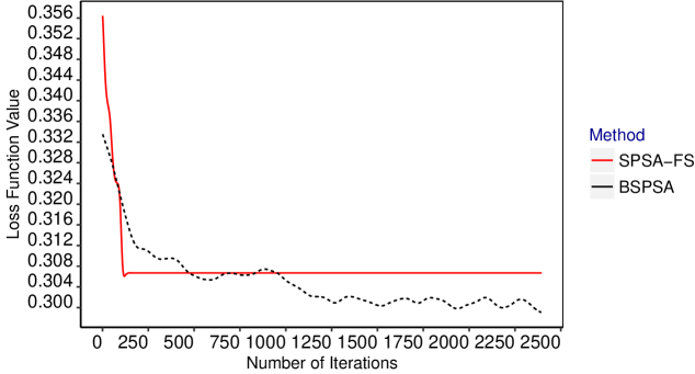
Figure 3.1: Covergence Time Comparison between SPSA-FS and BSPSA on Arrhythmia dataset. Using decision-tree, SPSA-FS hit its lowest loss function value before reaching 250 iterations. BSPSA required around 500 iterations to achieve the same loss function value although it outperformed the SPSA-FS algorithm if more iterations were allowed.

Chapter 4 Wrapper Comparison

Supervised learning problems can fall into two broad categories: classification and regression. The target or dependent feature is a binary, nominal or ordinal variable in a classification task while it is a continuous variable in a regression problem. Apart from feature selection, classification problems have another important aspect: feature ranking. While feature selection aims to determine the optimal subset of predictive features, feature ranking measures how important each feature from the specified set explains the target feature. For comparability, we divided the wrapper comparison experiments into three sections below:

• Feature Selection in Classification Problems

• Feature Ranking in Classification Problems

• Feature Selection in Regression Problems

We ran the wrapper comparison experiments using the open dataset accessible from the following sources:

• UCI Machine Learning Repository (Lichman 2013)

• DCC Regression DataSets (Torgo 2017)

• Scikit-feature feature selection repository at ASU (J. Li et al. 2016)

4.1 Feature Selection in Classification Problems

We selected nine (9) datasets for feature selection (see Table 4.1). For each dataset, we implemented four classifiers namely Recursive Partitioning for Classification (R.Part), K-Nearest Neighbours (KNN), Naïve Bayes (NB), and Support Vector Machine (SVM). For each classifier, we considered three main wrapper methods:

• SPSA;

• SFS: Sequential feature selection; and

• Full as the baseline benchmark.

For some datasets, we compared four following additional wrappers below:

• GA: Genetic Algorithm;

• SBS: Sequential Backward Selection;

• SFFS: Sequential Feature Forward selection; and

• SFBS: Sequential Feature Backward selection.

Besides the mean classification error rate, we also considered the mean runtime of the learning process to assess feature selection performance. Despite the mixed results, SPSA-FS managed to balance accuracy and runtime on average. In the scenario where SPSA-FS outperformed in the accuracy, it required slightly more or approximately runtime of other wrappers. When SPSA-FS trailed behind other wrappers in term of accuracy, it did not cost too much runtime. Such empirical results were consistent with the theoretical design of SPSA-FS where the BB method helps reduce the computational cost by sacrificing a minimal amount of accuracy.

dataset	$p$	$N$	Source	Figure
Arrhythmia	279	452	UCI	Figure 4.1
Glass	9	214	UCI	Figure 4.2
Heart	13	270	UCI	Figure 4.3
Ionosphere	34	351	UCI	Figure 4.4
Libras	90	360	UCI	Figure 4.5
Musk (Version 1)	166	476	UCI	Figure 4.6
Sonar	60	208	UCI	Figure 4.7
Spam Base	57	4601	UCI	Figure 4.8
Vehicle	18	946	UCI	Figure 4.9

Table 4.1: Feature Selection Classification datasets. $p$ represents the number of explanatory feature excluding exclude the response variables and identifier attributes; $N$ denotes the number of observations.

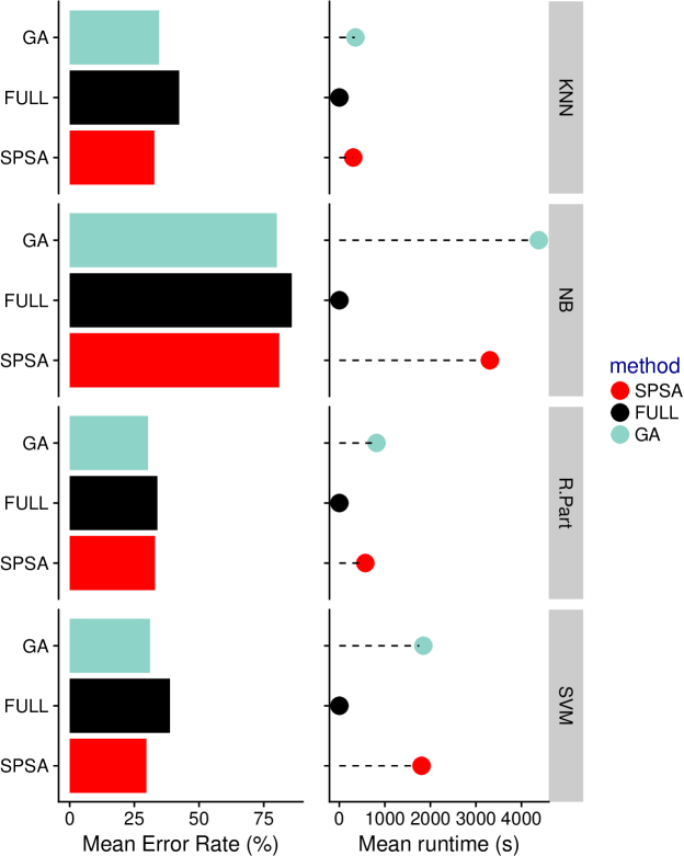
Figure 4.1: Feature Selection Performance Result on Arrhythmia

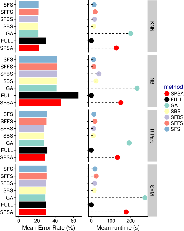
Figure 4.2: Feature Selection Performance Result on Glass

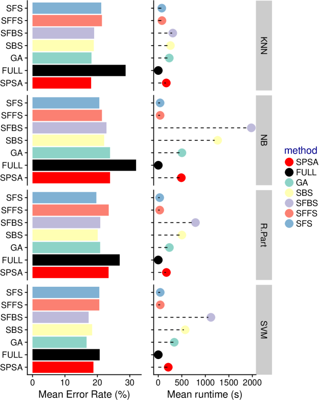
Figure 4.3: Feature Selection Performance Result on Heart

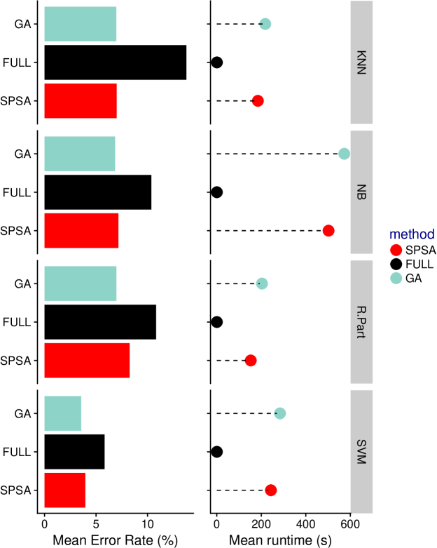
Figure 4.4: Feature Selection Performance Result on Ionospehere

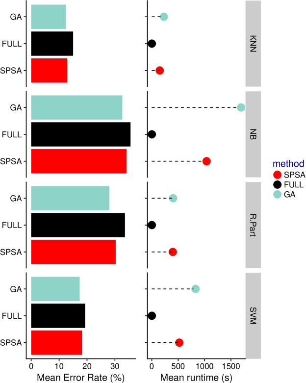
Figure 4.5: Feature Selection Performance Result on Libras

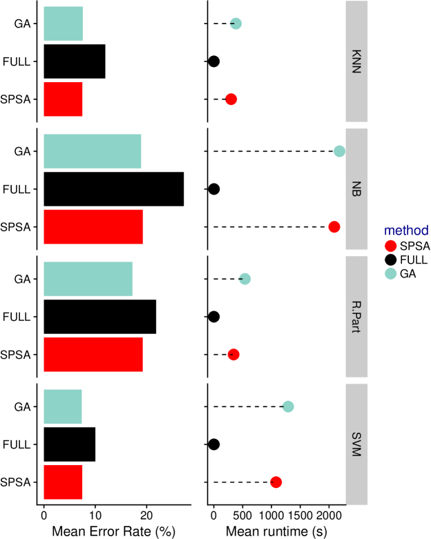
Figure 4.6: Feature Selection Performance Result on Musk

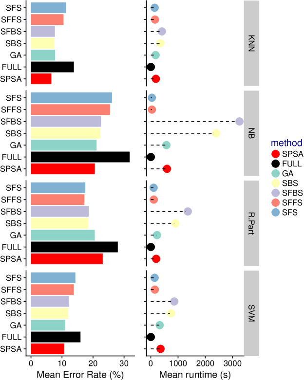
Figure 4.7: Feature Selection Performance Result on Sonar

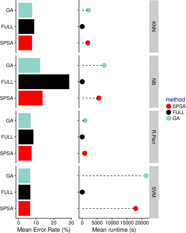
Figure 4.8: Feature Selection Performance Result on Spam Base

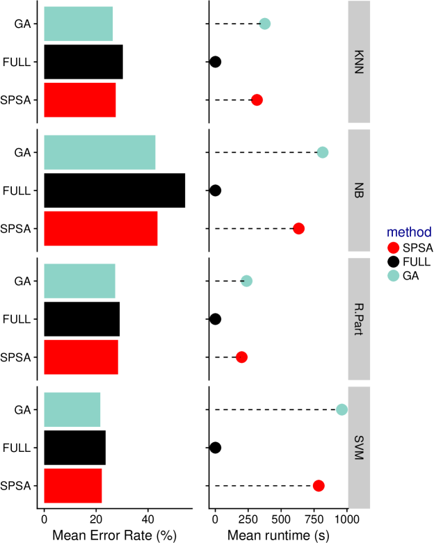
Figure 4.9: Feature Selection Performance Result on Vehicle

4.2 Feature Ranking in Classification Problems

Table 4.2 delineates eight (8) datasets for feature ranking. For each dataset, we applied four (4) classifiers which were Decision Tree (DT), K-Nearest Neighbours (KNN), Naïve Bayes (NB), and Support Vector Machine (SVM). For each classifier, using the mean classification error rate, we compared five wrapper methods below:

• SPFS: SPSA as Feature Selection;

• RFI: Random Forest Importance;

• Chi.Sq: Chi-Squared;

• Info.Gain: Information Gain; and

• Full as the baseline benchmark.

As shown in Table 4.2, each dataset has a large number of features, especially Orl and AR10p which suffer the high dimensionality curse, i.e. $p>N$. To illustrate the difference in feature ranking by wrappers, we capped the number of features used say $m$ in each classifier and utilised each wrapper to return the top $m$ important features. For example, consider Sonar dataset which consists of 60 features and $m=5$. Each wrapper would rank the top 5 important features out of 60 which yield the lowest accuracy rate in classifying the type of rock from Sonar data.

For completeness, we ran the experiment on a series of $m$ starting from 5 up to 40 features in an increment of 5. That is, $m=\{5,10,15,...,40\}$. We also compared the wrapper performance to the baseline benchmark, which incorporated all features. Unlike $R^{2}$ used in regression problems, additional explanatory features do not necessarily improve the accuracy rate. For example, as depicted in Figure 4.10, NB classifier committed more misclassifications on Sonar data when more than 30 features were used in each wrapper.

From Figures 4.10 to 4.17, we inferred that:

1. With some exceptions, the accuracy rates tended to decrease as the number of features increased albeit at a lower rate.

2. SPSA-FS outperformed other wrapper methods in most data sets but did not consistently beat the baseline due to the choice of classifier.

Dataset	$p$	$N$	Source	Figure
Sonar	60	208	UCI	Figure 4.10
Libras	90	360	UCI	Figure 4.11
Musk (Version 1)	166	476	UCI	Figure 4.12
Usps	256	9298	ASU	Figure 4.13
Isolet	617	1560	ASU	Figure 4.14
Coil20	1024	1440	ASU	Figure 4.15
Orl	1024	400	ASU	Figure 4.16
AR10p	2400	130	ASU	Figure 4.17

Table 4.2: Feature Ranking Classification datasets. $p$ represents the number of explanatory feature excluding exclude the response variables and identifier attributes; $N$ denotes the number of observations.

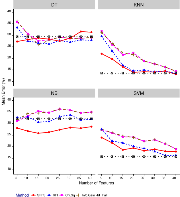
Figure 4.10: Wrapper Misclassification Error on Sonar dataset by Types of Classifiers

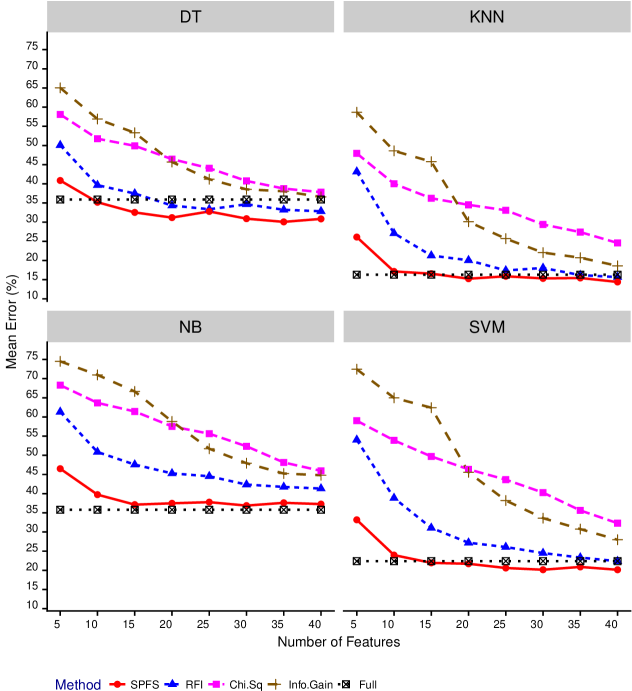
Figure 4.11: Wrapper Misclassification Error on Libras dataset by Types of Classifiers

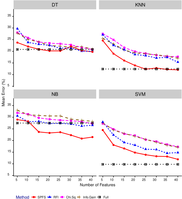
Figure 4.12: Wrapper Misclassification Error on Musk dataset by Types of Classifiers

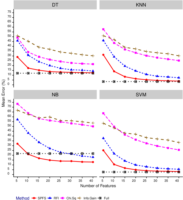
Figure 4.13: Wrapper Misclassification Error on USPS dataset by Types of Classifiers

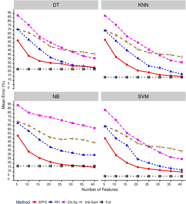
Figure 4.14: Wrapper Misclassification Error on Isolet dataset by Types of Classifiers

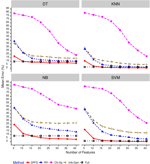
Figure 4.15: Wrapper Misclassification Error on Coil20 dataset by Types of Classifiers

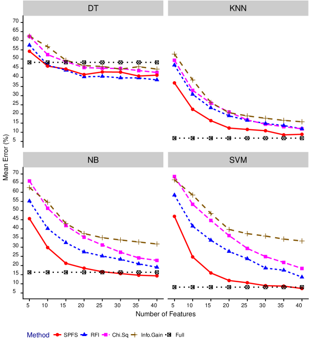
Figure 4.16: Wrapper Misclassification Error on Orl dataset by Types of Classifiers

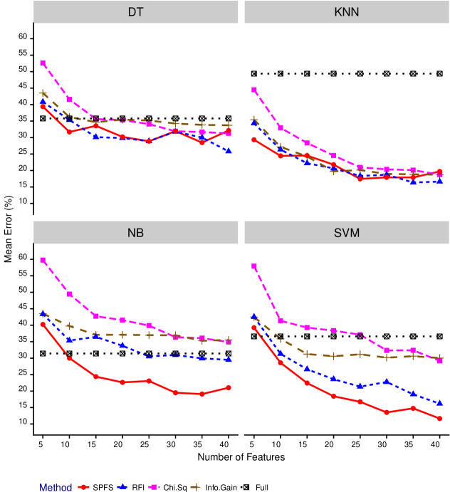
Figure 4.17: Wrapper Misclassification Error on AR10p dataset by Types of Classifiers

4.3 Feature Selection in Regression Problems

The regression experiment involved eight datasets. Table 4.3 describes each dataset and their sources. Using a typical linear regression model, we ran the following feature selection methods for each dataset:

• SPSA-FS

• Minimum Redundancy Maximum Relevance (mRMR), proposed by C. Ding and Peng (2003)

• RELIEF algorithm, which is first introduced by Kira and Rendell (1992)

• Linear Correlation

Dataset	$p$	$N$	Source	Figure
Ailerons	39	13750	DCC	Figure 4.18
CPU ACT	21	8192	DCC	Figure 4.19
Elevator	17	16559	DCC	Figure 4.20
Boston Housing	13	506	UCI	Figure 4.21
Pole Telecomm	47	1500	DCC	Figure 4.22
Pyrim	26	74	DCC	Figure 4.23
Triazines	58	186	DCC	Figure 4.24
Wisconsin Breast Cancer	32	194	UCI	Figure 4.25

Table 4.3: Regression datasets. $p$ represents the number of explanatory feature excluding exclude the response variables and identifier attributes; $N$ denotes the number of observations.

For benchmarking, we calculated inaccuracy rate defined by $1-R^{2}$ (R-squared) with respect to the number of features used in the regression. Known as the coefficient of determination, $R^{2}$ measures how close the data are to the fitted regression line. Therefore, a higher $R^{2}$ implies a lower inaccuracy rate. Note that $R^{2}$ can only either increase or remain constant as the number of explanatory variables or features, $p$ increases. For comparative evaluation, we normalised $p$ to the percentage of features used since each dataset has a different number of explanatory features. In all datasets, on average, SPSA-FS outperformed other wrapper methods even with fewer features. Other wrapper methods would only catch up with SPSA-FS starting 30 % of explanatory features used. At 100 %, i.e. when all explanatory features were used as regressors, all wrapper methods converged to approximately similar inaccuracy rate due to the nature of $R^{2}$. The exemplary performance of SPSA-FS implies it managed to identify the optimal subset of regressors given the same number of explanatory features compared to other methods.

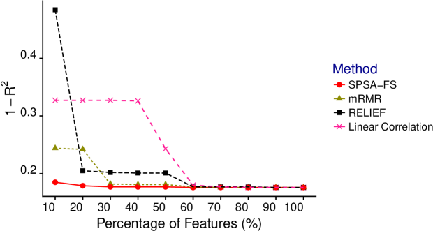
Figure 4.18: Regression On Ailerons

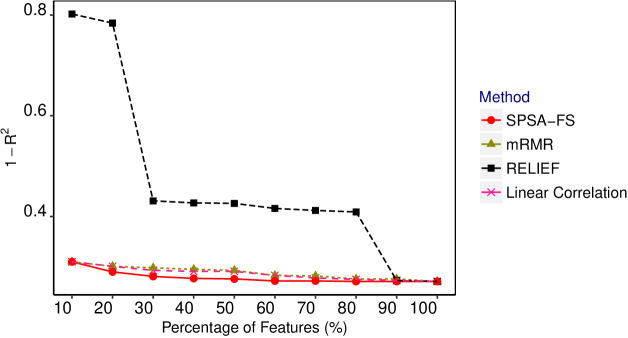
Figure 4.19: Regression On CPU ACT

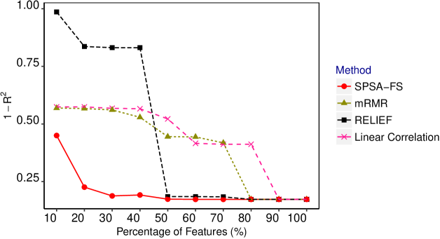
Figure 4.20: Regression on Elevators

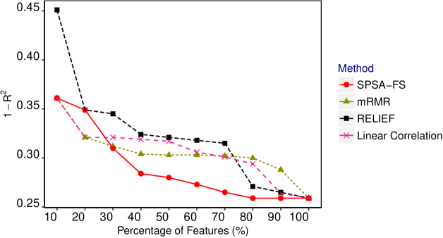
Figure 4.21: Regression on Boston Housing

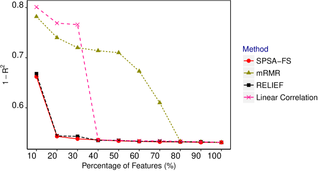
Figure 4.22: Regression on Pole Telecom

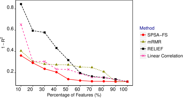
Figure 4.23: Regression on Pyrim

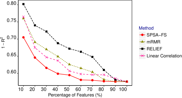
Figure 4.24: Regression on Triazines

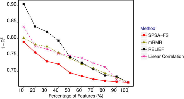
Figure 4.25: Regression on Wisconsin Breast Cancer

Chapter 5 Summary and Conclusions

In this study, we propose the SPSA-FS algorithm which mitigates the slow convergence issue of the BSPSA algorithm in feature selection. By applying BB method to smooth step size and average gradient estimates, SPSA-FS results in significantly lower computational costs but a very minimal loss of accuracy. To vindicate our proposition, we ran experiments which compared SPSA-FS to other wrapper methods on various open datasets. For classification tasks, we evaluated accuracy performance of the wrappers using the misclassification error rate. The results were mixed since SPSA-FS’s performance relied on the choice of the classifier. However, SPSA-FS managed to strike a balance between runtime required and accuracy. In the situation where SPSA-FS outperformed, it yielded significantly higher accuracy rate. Meanwhile, in the scenario where it underperformed, the performance differences were marginal. For regression tasks, by using one minus R-squared as the error measure, and SPSA-FS outperformed other wrappers with fewer explanatory features. In conclusion, theoretically and empirically, SPSA-FS not only leverages on the design of BSPSA which yields optimal feature selection results but also gains substantial speed in locating the solutions.

References

Aksakalli, Vural, and Milad Malekipirbazari. 2016. “Feature Selection via Binary Simultaneous Perturbation Stochastic Approximation.” Pattern Recognition Letters 75 (Supplement C): 41–47. doi:https://doi.org/10.1016/j.patrec.2016.03.002.

Al-Ani, Ahmed. 2005. “Feature Subset Selection Using Ant Colony Optimization.” International Journal of Computational Intelligence 2 (January): 53–58.

Apolloni, Javier, Guillermo Leguizamón, and Enrique Alba. 2016. “Two Hybrid Wrapper-Filter Feature Selection Algorithms Applied to High-Dimensional Microarray Experiments.” Applied Soft Computing 38: 922–32.

Barzilai, J., and J. Borwein. 1988. “Two-Point Step Size Gradient Methods.” IMA Journal of Numerical Analysis 8: 141–48.

Bennasar, Mohamed, Yulia Hicks, and Rossitza Setchi. 2015. “Feature Selection Using Joint Mutual Information Maximisation.” Expert Systems with Applications 42: 8520–32.

Cadenas, Jose M., M. Carmen Garrido, and Raquel Martinez. 2013. “Feature Subset Selection Filter–Wrapper Based on Low Quality Data.” Expert Systems with Applications 40: 6241–52.

Cauchy, M. Augustine. 1847. “Méthode Générale Pour La Résolution Des Systèmes d’équations Simultanées.” Comptes Rendus Hebd. Seances Acad. Sci. 25: 536–38.

Chen, Yu-Peng, Ying Li, Gang Wang, Yue-Feng Zheng, Qian Xu, Jia-Hao Fan, and Xue-Ting Cui. 2017. “A Novel Bacterial Foraging Optimization Algorithm for Feature Selection.” Expert Systems with Applications 83: 1–17.

Dai, Y., and L. Liao. 2002. “R-Linear Convergence of the Barzilai and Borwein Gradient Method.” IMA Journal of Numerical Analysis 22: 1–10.

Dai, Y., W. Hager, K. Schittkowski, and H. Zhang. 2006. “The Cyclic Barzilai-Borwein Method for Unconstrained Optimization.” Journal of Numerical Analysis 26: 604–27.

Debuse, J. C. W., and V. J. Rayward-Smith. 1997. “Feature Subset Selection Within a Simulated Annealing Data Mining Algorithm.” Journal of Intelligent Information Systems 9 (January): 57–81.

Ding, C., and H. Peng. 2003. “Minimum Redundancy Feature Selection from Microarray Gene Expression Data.” In Computational Systems Bioinformatics. Csb2003. Proceedings of the 2003 Ieee Bioinformatics Conference. Csb2003, 523–28. doi:10.1109/CSB.2003.1227396.

Ghaemi, Manizheh, and Mohammed-Reza Feizi-Derakhshi. 2016. “Feature Selection Using Forest Optimization Algorithm.” Pattern Recognition 60: 121–29.

Guvenir, H A, B Acar, G Demiroz, and A Cekin. 1997. “A Supervised Machine Learning Algorithm for Arrhythmia Analysis.” In Computers in Cardiology, 433–36.

Guyon, I., and Andre Elisseeff. 2003. “An Introduction to Variable and Feature Selection.” Journal of Machine Learning Research 3: 1157–82.

Guyon, I., J. Weston, S. Barnhill, and V. Vapnik. 2002. “Gene Selection for Cancer Classifica- Tion Using Support Vector Machines.” Machine Learning 46: 389–422.

Hsu, Hui-Huang, Cheng-Wei Hsieh, and Lu Ming-Da. 2011. “Hybrid Feature Selection by Combining Filters and Wrappers.” Expert Systems with Applications 38: 8144–50.

Kira, Kenji, and Larry A. Rendell. 1992. “The Feature Selection Problem: Traditional Methods and a New Algorthm.” In AAAI-92 Proceedings.

Kohavi, R., and G. H. John. 1997. “Wrappers for Feature Subset Selection.” Artificial Intelligence 97 (1-2): 273–324.

Leo, B. 2001. “Random Forests.” Machine Learning 45: 5–32.

Li, Jundong, Kewei Cheng, Suhang Wang, Fred Morstatter, Trevino Robert, Jiliang Tang, and Huan Liu. 2016. “Feature Selection: A Data Perspective.” arXiv:1601.07996.

Lichman, M. 2013. “UCI Machine Learning Repository.” University of California, Irvine, School of Information; Computer Sciences. http://archive.ics.uci.edu/ml.

Lu, Huijuan, Junying Chen, Ke Yan, Qun Jin, Yu Xue, and Zhigang Gao. 2017. “A Hybrid Feature Selection Algorithm for Gene Expression Data Classification.” Neurocomputing 256: 56–62.

Mafarja, Majdi M., and Seyedali Mirjalili. 2017. “Hybrid Whale Optimization Algorithm with Simulated Annealing for Feature Selection.” Neurocomputing 260: 302–12.

Molina, B, and M Raydan. 1996. “Preconditioned Barzilai-Borwein Method for the Numerical Solution of Partial Differential Equations.” Numerical Algorithms 13: 45–60.

Nocedal, Jorge, and Stephen J. Wright. 2006. Numerical Optimization. 2nd ed. Newyork: Springer.

Oluleye, B., L. Armstrong, and D. Diepeveen. 2014. “A Genetic Algorithm-Based Feature Selectionture Selection.” International Journal of Electronics Communication and Computer Engineering 5 (April): 2278–4209.

Ólafsson, Sigurdur, and Jaekyung Yang. 2005. “Intelligent Partitioning for Feature Selection.” INFORMS Journal on Computing 17 (3): 339–55.

Pashaei, Elnaz, and Nizamettin Aydin. 2017. “Binary Black Hole Algorithm for Feature Selection and Classification on Biological Data.” Applied Soft Computing 56: 94–106.

Peng, H., F. Long, and C. Ding. 2005. “Feature Selection Based on Mutual Information: Criteria of Max-Dependency, Max-Relevance, and Min-Redundancy.” IEEE Transactions on Pattern Analysis and Machine Intelligence, no. 1226–1238.

Pudil, P., J. Novovicová, and J. Kittler. 1994. “Floating Search Methods in Feature Selection.” Pattern Recognition Letters 15 (October): 1119–25.

R Core Team. 2017. R: A Language and Environment for Statistical Computing. Vienna, Austria: R Foundation for Statistical Computing. https://www.R-project.org/.

Raydan, M. 1993. “On the Barzilai and Borwein Choice of Steplength for the Gradient and Method.” IMA Journal of Numerical Analysis 13: 321–26.

Raydan, M, and B. Svaiter. 2002. “Relaxed Steepest Descent and Cauchy-Barzilai-Borwein Method.” Computational Optimization and Applications 21: 155–67.

Raymer, Michael L., William F. Punch, Erik D. Goodman, Leslie Kuhn, Anil K. Jain, and et al. 2000. “Dimensionality Reduction Using Genetic Algorithms.” Evolutionary Computation, IEEE Transactions on 4 (February): 164–71.

Sayed, Safinaz AbdEl-Fattah, Emad Nabil, and Amr Badr. 2016. “A Binary Clonal Flower Pollination Algorithm for Feature Selection.” Pattern Recognition Letters 77: 21–27.

Senawi, Azlyna, Hua-Liang Wei, and Stephan A. Billings. 2017. “A New Maximum Relevance-Minimum Multicollinearity (Mrmmc) Method for Feature Selection and Ranking.” Pattern Recognition 67: 47–61.

Sikonia, M. R., and I. Kononenko. 2003. “Theoretical and Empirical Analysis of Relief and Relieff.” Machine Learning 53 (23-69).

Spall, James C. 1992. “Multivariate Stochastic Approximation Using a Simultaneous Perturbation Gradient Approximation.” IEEE 37 (3): 322–41.

Spall, James C. 2003. ’Introduction to Stochastic Search and Optimization: Estimation, Simulation, and Control’. John Wiley.

Spall, James C., and Wang Qi. 2011. “Discrete Simultaneous Perturbation Stochastic Approximation on Loss Function with Noisy Measurements.” ’In: Proceeding American Control Conference’ 37 (3): 4520–5.

Tahir, M. A., A. Bouridane, and F. Kurugollu. 2007. “Simultaneous Feature Selection and Feature Weighting Using Hybrid Tabu Search/K-Nearest Neighbor Classifier.” Pattern Recognition Letters 28 (April): 438–46.

Tan, Conghui, Shiqian Ma, Yu-Hong Dai, and Yuqiu Qian. 2016. “Barzilai-Borwein Step Size for Stochastic Gradient Descent.” Barcelona.

Tibshirani, Robert. 1996. “Regression Shrinkage and Selection via the Lasso.” Journal of the Royal Statistical Society, Series B 58: 267–88.

Torgo, L. 2017. “DCC Regression Datasets.” Universidade Do Porto, Portugal, Department of Computer Science. http://www.dcc.fc.up.pt/~ltorgo/Regression/DataSets.html.

Tsai, Chih-Fong, William Eberle, and Chi-Yuan Chu. 2013. “Genetic Algorithms in Feature and Instance Selection.” Knowledge-Based Systems 39: 240–47.

Wan, Youchuan, Mingwei Wang, Zhiwei Ye, and Xudong Lai. 2006. “A Feature Selection Method Based on Modified Binary Coded Ant Colony Optimization Algorithm.” Applied Soft Computing 49: 248–58.

Wang, Lipo, Yaoli Wang, and Qing Chang. 2016. “Feature Selection Methods for Big Data Bioinformatics: A Survey from the Search Perspective.” Methods 111 (December): 21–31.

Wang, X., J. Yang, X. Teng, W Xia, and R. Jensen. 2007. “Feature Selection Based on Rough Sets and Particle Swarm Optimization.” Pattern Recognition Letters 28 (April): 459–71.

Wickham, Hadley. 2016. Ggplot2: Elegant Graphics for Data Analysis. Springer-Verlag New York. http://ggplot2.org.

Xie, Yihui. 2015. Dynamic Documents with R and Knitr. 2nd ed. Boca Raton, Florida: Chapman; Hall/CRC. https://yihui.name/knitr/.

Zheng, Zhonglong, Xie Chenmao, and Jiong Jia. 2010. “ISO-Container Projection for Feature Extraction.” IEEE.