Probabilistic Rewriting and Asymptotic Behaviour:
on Termination and Unique Normal Forms

Abstract.

While a mature body of work supports the study of rewriting systems, abstract tools for Probabilistic Rewriting are still limited. In this paper we study the question of uniqueness of the result (unique limit distribution), and develop a set of proof techniques to analyze and compare reduction strategies. The goal is to have tools to support the operational analysis of probabilistic calculi (such as probabilistic lambda-calculi) where evaluation allows for different reduction choices (hence different reduction paths).

1. Introduction

Rewriting Theory [Ter03] is a foundational theory of computing. Its impact extends to both the theoretical side of computer science, and the development of programming languages. A clear example of both aspects is the paradigmatic term rewriting system, $\lambda$-calculus, which is also the foundation of functional programming. Abstract Rewriting Systems (ARS) are the general theory which captures the common substratum of rewriting theory, independently of the particular structure of the objects. It studies properties of terms transformations, such as normalization, termination, unique normal form, and the relations among them. Such results are a powerful set of tools which can be used when we study the computational and operational properties of any calculus or programming language. Furthermore, the theory provides tools to study and compare strategies, which become extremely important when a system may have reductions leading to a normal form, but not necessarily. Here we need to know: is there a strategy which is guaranteed to lead to a normal form, if any exists (normalizing strategies)? Which strategies diverge if at all possible (perpetual strategies)?

Probabilistic Computation models uncertainty. Probabilistic forms of automata [Rab63], Turing machines [San71], and the $\lambda$-calculus [Sah78] exist since long. The pervasive role it is assuming in areas as diverse as robotics, machine learning, natural language processing, has stimulated the research on probabilistic programming languages, including functional languages [KMP97, RP02, PPT05] whose development is increasingly active. A typical programming language supports at least discrete distributions by providing a probabilistic construct which models sampling from a distribution. This is also the most concrete way to endow the $\lambda$-calculus with probabilistic choice [DPHW05, DLZ12, EPT11]. Within the vast research on models of probabilistic systems, we wish to mention that probabilistic rewriting is the explicit base of PMaude [AMS06], a language for specifying probabilistic concurrent systems.

Probabilistic Rewriting. Somehow surprisingly, while a large and mature body of work supports the study of rewriting systems—even infinitary ones [DKP91, KKSdV95]—work on the abstract theory of probabilistic rewriting systems is still sparse. The notion of Probabilistic Abstract Reduction Systems (PARS) has been introduced by Bournez and Kirchner in [BK02], and then extended in [BG06] to account for non-determinism. Recent work [LFVY17, DM18, KC17, ALY20] shows an increased research interest. The key element in probabilistic rewriting is that even when the probability that a term leads to a normal form is $1$ (almost sure termination, AST), that degree of certitude is typically not reached in any finite number of steps, but it appears as a limit. Think of a rewrite rule (as in Fig. 3) which rewrites $c$ to either the value T or $c$, with equal probability $1/2$. We write this as $c\rightarrow\{c^{1/2},{\texttt{T}}^{1/2}\}$. After $n$ steps, $c$ reduces to T with probability $\frac{1}{2}+\frac{1}{2^{2}}+\cdots+\frac{1}{2^{n}}$. Only at the limit this computation terminates with probability $1$.

The most well-developed literature on PARS is concerned with methods to prove almost sure termination, see e.g. [BG06, FH15, HFCG19, ALY20] (this interest matches the fact that there is a growing body of methods to establish AST [ACN18, FC19, KKMO18, MMKK18, LFR21]). However, considering rewrite rules subject to probabilities opens numerous other questions, which motivate our investigation.

We study a rewrite relation which describes the global evolution of a probabilistic system, for example a probabilistic program $P$. The result of the computation is a probability distribution $\beta$ over all the possible output of $P$. The intuition (see [KMP97]) is that the program $P$ is executed, and random choices are made by sampling. This process defines a distribution $\beta$ over the various outputs that the program can produce. We write this $P\xRightarrow{\infty}\beta$.

What happens if the evaluation of a term $P$ is not deterministic, in the sense that different reduction choices are available? Remember that non-determinism arises naturally in the $\lambda$-calculus, because a term may have several redexes. This aspect has practical relevance to programming. Together with the fact that the result of a terminating computation is unique, (independently from the evaluation choices), it is key to the inherent parallelism of functional programs (see e.g. [Mar13]).

Assume program $P$ generates a distribution over booleans $\{{\texttt{T}}^{\frac{1}{16}},{\texttt{F}}^{\frac{15}{16}}\}$; it is desirable that the distribution which is computed is unique: it only depends on the “input” (the problem), not on the way the computational steps are performed.

When assuming non-deterministic evaluation, several questions on PARS arise naturally. For example: (1.) when—and in which sense—is the result unique? (naively, if $P\xRightarrow{\infty}\alpha$ and $P\xRightarrow{\infty}\beta$, is $\alpha=\beta$?) (2.) Do all rewrite sequences from the same term have the same probability to reach a result? (3.) If not, does there exist a strategy to find a result with greatest probability?

Such questions are relevant to the theory and to the practice of computing. We believe that to study them, we can advantageously adapt techniques from Rewrite Theory. However, we cannot assume that standard properties of ARSs hold for PARSs. The game-changer is that termination appears as a limit. In Section 4.2.3 we show that a well-known ARSs property, Newman’s Lemma, does not hold for PARSs. This is not surprising; indeed, Newman’s Lemma is known not to hold in general for infinitary rewriting [Ken92, KdV05]. Still, our counter-example points out that moving from ARS to PARS is non-trivial. There are two main issues: we need to find the right formulation and the right proof technique. It seems then especially important to have a collection of proof methods which apply well to PARS.

Content and contributions.

Probability is concerned with asymptotic behaviour: what happens not after a finite number $n$ of steps, but when $n$ tends to infinity. In this paper we focus on the asymptotic behaviour of rewrite sequences with respect to normal forms—normal form being the most standard notion of result in rewriting. We study computational properties such as (1.), (2.), (3.) above. We do so with the point of view of ARSs, aiming for properties which hold independently of the specific nature of the rewritten objects; the purpose is to have tools which apply to any probabilistic rewriting system.

PARS.

After motivating and introducing our formalism for PARSs (Section 2 and 3), in Section 4 we formalize the notion of limit distribution, and of well-defined result. Since in a PARS each term has different possible reduction sequences (with each sequence leading to a possibly different limit distribution), to each term is naturally associated a set of limit distributions. To study when a PARS has a well-defined result is the main focus of the paper.

Recall a property which is crucial to the computational interpretation of a system such as the $\lambda$-calculus: if a term has a normal form, it is unique—meaning that the result of the computation is well-defined. With this in mind, we investigate in the probabilistic setting an analogue of the ARS notions of Unique Normal Form (UN), and the possibility or necessity to reach a result: Normalization (WN), Termination (SN). We provide methods and criteria to establish these properties, and we uncover relations between them. Specific contributions are the following.

• We propose an analogue of UN  for PARS. The question was already studied in [DM18] for PARS which are almost surely terminating, but the solution there does not extend to the general case.

• We investigate the classical ARS method to prove UN via confluence; we uncover that subtle aspects appear when dealing with a notion of result as a limit. We do prove an analogue of “confluence implies UN” for PARS—however the proof is not simply an adaptation of the standard techniques, due to the fact that the set of limit distributions is—in general—infinite, and it is not guaranteed to have maximal elements (think of ${[0,1[}$ which has a sup, but not a max).

Asymptotic rewriting: QARS.

To better understand the asymptotic behaviour of computation, in Section 5 we introduce the setting of Quantitative Abstract Rewrite System (QARS). While motivated from the analysis of probabilistic rewriting, QARSs abstract from the probabilistic structure. This allows us to capture the essence of the arguments, and to separate the properties which really depend on probability (and its specific properties) from those which are only concerned with the fact that results are limits.

QARS are a natural refinement of the notion of Abstract Rewrite Systems with Information content (ARSI), introduced by Ariola and Blom [AB02]. There, to the ARS is associated a partial order that expresses the information content of the elements. We adopt the same view. ARSI however have a notion of limit which is tailored to infinite normal forms in the sense of Böhm trees [Bar84] and Levy-Longo trees [Lév78]. With QARS, we simply move from partial orders (and a specific definition of limit), to $\omega$-complete partial orders—this is enough to capture also probabilistic computation.

First, we study the properties of limits. Then, we provide a set of proof techniques to support the asymptotic analysis of reduction strategies. To do so, we extend to our setting a method which was introduced for ARSs by Van Oostrom [vO07], and which is based on Newman’s property of Random Descent (RD) [New42, vO07, vOT16] (see Section 1.1.2). The Random Descent method turns out to be well-suited to asymptotic and probabilistic rewriting, providing a useful family of tools. In analogy to their counterpart in [vO07], we generalize in a quantitative way the notions of Random Descent (which becomes $\mathtt{obs}$-RD) and of being better (which become $\mathtt{obs}\mbox{-better}$); both properties are here parametric with respect to the information content which we wish to observe.

A significant technical feature (inherited from [vO07]) is that both notions of $\mathtt{obs}$-RD and $\mathtt{obs}\mbox{-better}$ come with a characterization via a local condition, in the sense that only single steps from an object—rather than all possible sequences of steps—need to be examined.

Probabilistic rewriting: tools and applications.

In Sections 7 and 8 we specialize the Random Descent techniques to PARS.

• $\mathtt{obs}$-RD entails that all rewrite sequences from a term lead to the same result, in the same expected number of steps (the average of number of steps, weighted w.r.t. probability).

• $\mathtt{obs}\mbox{-better}$ offers a method to compare strategies (“strategy $\mathcal{S}$ is always better than strategy $\mathcal{T}$”) w.r.t. the probability of reaching a result and the expected time to reach a result. It provides a sufficient criterion to establish that a strategy is normalizing (resp. perpetual) i.e. the strategy is guaranteed to lead to a result with maximal (resp. minimal) probability.

To illustrate their use, we apply these methods to a probabilistic $\lambda$-calculus—Weak Call-by-Value $\lambda$-calculus—which is discussed in Section 7.2. A larger example of application to probabilistic $\lambda$-calculi is [FR19], whose developments rely also on the abstract results presented here; we illustrate this in Section 9.

Remark 1 (On the term Random Descent).

Please note that in [New42], the term Random refers to non-determinism (in the choice of the redex), not to randomized choice.

Journal vs conference version.

This paper is the journal version of [Fag19]. The content has been considerably extended. In particular, we develop the setting of QARS (Section (5)), which formalizes the notion of asymptotic rewriting, and does not appear in [Fag19]. This allows us to separate the properties which really depend on probability from those which are concerned with results as limits, cleaning the arguments from unnecessary structure. The study of limits in both probabilistic and non-probabilistic setting is unified to a more general theory. The results obtained for QARS can be transferred to ARS and PARS alike, but also to other frameworks where reduction is asymptotic.

1.1. Motivations and Background

1.1.1. Probabilistic $\lambda$-calculus, non-deterministic evaluation,
and (non-)Unique Result

Rewrite theory provides numerous tools to study uniqueness of normal forms, as well as techniques to study and compare strategies. This is not the case in the probabilistic setting. Perhaps a reason is that when extending the $\lambda$-calculus with a choice operator, confluence is lost, as was observed early [dP95]; we illustrate it in Example 1.1.1 and 1.1.1, which is adapted from [dP95, DLZ12]. The way to deal with this issue in probabilistic $\lambda$-calculi (e.g. [DPHW05, DLZ12, EPT11]) has been to fix a deterministic reduction strategy, typically “leftmost-outermost”. To fix a deterministic strategy is not satisfactory, neither for the theory nor the practice of computing. To understand why this matters, recall for example that confluence of the $\lambda$-calculus is what makes functional programs inherently parallel: every sub-expression can be evaluated in parallel, still, we can reason on a program using a deterministic sequential model, because the result of the computation is independent of the evaluation order (we refer to [Mar13], and to Harper’s text “Parallelism is not Concurrency” for discussion on deterministic parallelism, and how it differs from concurrency). Let us see what happens in the probabilistic case. [Confluence failure] Let us consider the untyped $\lambda$-calculus extended with a binary operator $\oplus$ which models probabilistic choice. Here $\oplus$ is just flipping a fair coin: $M\oplus N$ reduces to either $M$ or $N$ with equal probability $1/2$; we write this as $M\oplus N\rightarrow\{M^{\frac{1}{2}},N^{\frac{1}{2}}\}$.

Consider the term $PQ$, where $P=(\lambda x.x)(\lambda x.x\mathtt{~{}XOR~{}}x)$ and $Q=({\texttt{T}}\oplus{\texttt{F}})$; here $\mathtt{~{}XOR~{}}$ is the standard constructs for the exclusive $\mathtt{OR}$, T and F are terms which encode the booleans.

• If we evaluate $P$ and $Q$ independently, from $P$ we obtain $\lambda x.(x\mathtt{~{}XOR~{}}x)$, while from $Q$ we have either T or F, with equal probability $1/2$. By composing the partial results, we obtain $\{({\texttt{T}}\mathtt{~{}XOR~{}}{\texttt{T}})^{\frac{1}{2}},({\texttt{F}}\mathtt{~{}XOR~{}}{\texttt{F}})^{\frac{1}{2}}\}$, and therefore $\{{\texttt{F}}^{1}\}$.

• If we evaluate $PQ$ sequentially, in a standard leftmost-outermost fashion, $PQ$ reduces to $(\lambda x.x\mathtt{~{}XOR~{}}x)Q$ which reduces to $({\texttt{T}}\oplus{\texttt{F}})\mathtt{~{}XOR~{}}({\texttt{T}}\oplus{\texttt{F}})$ and eventually to $\{{\texttt{T}}^{\frac{1}{2}},{\texttt{F}}^{\frac{1}{2}}\}$.

The situation becomes even more complex if we examine also the possibility of diverging; try the same experiment on the term $PR$, with $P$ as above, and $R=({\texttt{T}}\oplus{\texttt{F}})\oplus\Delta\Delta$ (where $\Delta=\lambda x.xx$). Proceeding as before, we now obtain either $\{{\texttt{F}}^{\frac{1}{2}}\}$ or $\{{\texttt{T}}^{\frac{1}{8}},{\texttt{F}}^{\frac{1}{8}}\}$.

We do not need to loose the features of $\lambda$-calculus in the probabilistic setting. In fact, while some care is needed, determinism of the evaluation can be relaxed without giving up uniqueness of the result: the calculus we introduce in Section 7.2 is an example (we relax determinism to Random Descent); we fully develop this direction in further work [FR19]. To be able to do so, we need abstract tools and proof techniques to analyze probabilistic rewriting. The same need for theoretical tools holds, more in general, whenever we desire to have a probabilistic language which allows for deterministic parallel reduction.

In this paper we focus on uniqueness of the result, rather than confluence. While important, confluence is a sufficient but not necessary property to have uniqueness of normal forms.

1.1.2. Other key notions

Confluence is not enough.

Key to non-deterministic evaluation strategies is that, despite the fact that there are many ways of evaluating a term, all choices eventually yield the same result. To this aim, confluence is not enough. The reduction of a term that has a normal form may still produce diverging computations, which yield no result (think of $\beta$-reduction in usual $\lambda$-calculus, reducing the term $(\lambda x.z)(\Delta\Delta)$). What we really want for a non-deterministic evaluation strategy is that all reduction sequences from the same $\mathtt{t}$ have the same behaviour: if $\mathtt{t}$ has a normal form, then all reduction sequences from $\mathtt{t}$ eventually reach it (uniform normalization); ideally, all should do so in the same number of steps. This latter property is known as Random Descent [New42, vO07, vOT16], and it is often guaranteed in the literature of $\lambda$-calculus via a diamond-like property. We will lift these notions to the probabilistic and asymptotic setting.

Random Descent.

Newman’s Random Descent (RD) [New42] is an ARS property which guarantees that normalization suffices to establish both termination and uniqueness of normal forms. Precisely, if an ARS has random descent, paths to a normal form do not need to be unique, but they have unique length. In its essence: if a normal form exists, all rewrite sequences lead to it, and all have the same length. While only few systems directly verify it, RD is a powerful ARS tool; a typical use in the literature is to prove that a strategy has RD, to conclude that it is normalizing. A well-known property which implies RD is a form of diamond: $\leftarrow\cdot\rightarrow~{}\subseteq~{}(\rightarrow\cdot\leftarrow)~{}\cup~{}=$.

Von Oostrom [vO07] has defined a characterization of RD by means of a local property, proposing RD as a uniform method to (locally) compare strategies for normalization and minimality (resp. perpetuality and maximality). Such a method has then been extended in [vOT16], where the notion of length is abstracted into a notion of measure. In Section 7 and 8 we develop similar methods in a probabilistic setting. The probabilistic analogous of length, is the expected number of steps (Section 7.1).

Weak Call-by-Value $\lambda$-calculus (and its probabilistic counter-part).

A notable example of system which satisfies Random Descent is Call-by-Value (CbV) $\lambda$-calculus endowed with weak evaluation.

In Plotkin’s Call-by-Value $\lambda$-calculus, $\beta$-redexes are fired only when the argument is a value (i.e., a variable or a $\lambda$-abstraction). Since the goal is to compute values—as is natural in functional programming—evaluation is often restricted to be weak [How70, CH98], where weak means no reduction in the function bodies (i.e. within the scope of $\lambda$-abstractions). Weak CbV is the basis of the ML/CAML family of functional languages—and of most probabilistic functional languages. There are three main weak schemes: reducing from left to right, as originally defined by Plotkin [Plo75], from right to left, as in Leroy’s ZINC abstract machine [Ler90] (resulting in a more efficient implementation), or in an arbitrary order, used for example in [DLM08]. While left and right reduction are deterministic, weak reduction in arbitrary order is non-deterministic and subsumes both.

If we consider programs (closed terms), values are exactly the normal forms of weak reduction. Because it satisfies Random Descent, CbV weak reduction $\mathrel{\mathop{\rightarrow}\limits_{\vbox to0.0pt{\kern-6.0pt\hbox{$\scriptstyle\mathsf{w}$}\vss}}}$ has striking properties (see e.g. [DLM08] for an account). First, if $M$ reduces to a value ($M\mathrel{\mathop{\rightarrow}\limits_{\vbox to0.0pt{\kern-6.0pt\hbox{$\scriptstyle\mathsf{w}$}\vss}}}^{*}V$), then any sequence of $\mathrel{\mathop{\rightarrow}\limits_{\vbox to0.0pt{\kern-6.0pt\hbox{$\scriptstyle\mathsf{w}$}\vss}}}$-steps from $M$ will reach $V$; second, the number $n$ of steps such that $M\mathrel{\mathop{\rightarrow}\limits_{\vbox to0.0pt{\kern-6.0pt\hbox{$\scriptstyle\mathsf{w}$}\vss}}}^{n}V$ is always the same.

In Section 7.2, we study a probabilistic extension of weak CbV, $\Lambda_{\oplus}^{\mathsf{w}}$. We show that it has analogous properties to its classical counterpart: all rewrite sequences converge to the same result, in the same expected number of steps.

Local vs global conditions.

An important distinction in rewriting theory is between local and global properties. A property of a term $t$ is global if it is quantified over all rewrite sequences from $t$, it is local if it is quantified only over one-step reductions from the term. Local properties are easier to test, because the analysis (usually) involves a finite number of cases. To work locally—that is, reducing a test problem which is global to local properties—dramatically reduces the space of search when testing. Let us exemplify this with a familiar example.

A paradigmatic example of global property is confluence (CR): $b~{}{}^{*}\leftarrow a\rightarrow^{*}c$ $\Rightarrow$ $\exists d$ s.t. $b\rightarrow^{*}d~{}{}^{*}\leftarrow c$. Its global nature makes it difficult to establish. A standard way to factorize the problem is: (1.) prove termination and (2.) prove local confluence (WCR): $b\leftarrow a\rightarrow c$ $\Rightarrow$ $\exists d$ s.t. $b\rightarrow^{*}d~{}{}^{*}\leftarrow c$. This is exactly Newman’s lemma:  Termination + WCR $\Rightarrow$ CR. The beauty of Newman’s lemma is that a global property (CR) is guaranteed by a local property (WCR).

Locality is also the strength and beauty of the Random Descent method. While Newman’s lemma fails in a probabilistic setting, Random Descent methods adapt well.

1.2. Related work

First, let us observe that there is a vast literature on probabilistic transition systems, however objectives and therefore questions and tools are different than those of PARS. A similar distinction exist between abstract rewrite systems and transition systems. Here we discuss related work in the context of PARS [BG06, BK02].

We are not aware of any work which investigates normalizing strategies (or normalization in general, rather than termination). Instead, confluence in probabilistic rewriting has already drawn interesting work. A notion of confluence for a probabilistic rewrite system defined over a $\lambda$-calculus is studied in [DAGG11, DLMZ11]; in both cases, the probabilistic behaviour corresponds to measurement in a quantum system. The work more closely related to our goals is [DM18]. It studies confluence of non-deterministic PARS in the case of finitary termination (being finitary is the reason why Newman’s Lemma holds), and in the case of AST . As we observe in Section 4.2.2, their notion of unique limit distribution (if $\alpha,\beta$ are limits, then $\alpha=\beta$), while simple, it is not an analogue of UN for general PARS. We extend the analysis beyond AST, to the general case, which arises naturally when considering untyped probabilistic $\lambda$-calculus. On confluence, we also mention [KC17], whose results however do not cover non-deterministic PARS; the probability of the limit distribution is concentrated in a single element, in the spirit of Las Vegas Algorithms. [KC17] revisits results from [BK02], while we are in the non-deterministic framework of [BG06].

The way we define the evolution of a PARS, via the one-step relation $\mathrel{\rightrightarrows}$, follows the approach in [LFVY17], which also contains an embryo of the current work (a form of diamond property); the other results and developments are novel. A technical difference with [LFVY17] is that for the formalism to be general, a refinement is necessary (see Section 2.5); the issue was first pointed out in [DM18]. Our refinement is a variant of the one introduced (for the same reasons) in [ALY20]; there, normal forms are discarded—because the authors are only interested in the probability of termination—while we are interested in a more qualitative analysis of the result. [ALY20] demonstrates the equivalence with the approach in [BG06].

Quantitative Abstract Rewrite Systems (QARS) refine Ariola and Blom’s notion of Abstract Rewrite Systems with Information content (ARSI) [AB02]; there, to the ARS is associate a partial order which expresses a comparison between the “information content” of the elements. Here, we simply move from partial orders to $\omega$-complete partial orders ($\omega$-cpo). The difference is in the notion of limit, hence its properties, and our novel contribution is the study of such properties. ARSI are tailored to infinite normal forms in the sense of Böhm and Levy-Longo trees—limits (infinite normal forms) are there given by completing the partial order via a specific standard construction, ideal completion (see for instance Ch. 1 in [AC98]). So, given an element $\mathtt{t}$ in an ARSI, the infinite normal form of $\mathtt{t}$ is the downward closure of the set of the information contents of all its reducts. Such an approach would not suit probability distributions, but moving to $\omega$-cpo suffices. Being simply the supremum of an $\omega$-chain, the notion of limit which come with QARS is more general and flexible, allowing us to model a larger variety of situations. All results we establish for limits in the setting of QARS also hold for the infinite normal forms of ARSI, while the converse is not true. In Appendix A.1 we give a concrete example that shows the difference: a confluent ARSI has unique infinite normal forms (Theorem 5.4 there)—the analogue result is (in general) not true for QARS.

2. Probabilistic Abstract Rewriting System

We assume the reader familiar with the basic notions of rewrite theory (such as Ch. 1 of [Ter03]), and of discrete probability theory. We review the basic language of both. We then recall the definition of probabilistic abstract rewrite system from [BK02, BG06]—here denoted pars—and explain on examples how a system described by a pars evolves. This will motivate the formalism which we present in Section 3.

2.1. Basics on ARS

An abstract rewrite system (ARS) is a pair $\mathcal{C}=(C,\rightarrow)$ consisting of a set $C$ and a binary relation $\rightarrow$ on $C$ (called reduction) whose pairs are written $t\to s$ and called steps; $\rightarrow^{*}$ (resp. $\rightarrow^{=}$) denotes the transitive reflexive (resp. reflexive) closure of $\rightarrow$. We write $c\not\rightarrow$ if there is no $u$ such that $c\rightarrow u$; in this case, $c$ is a normal form. $\scalebox{0.6}[1.0]{NF}_{\mathcal{C}}$ denotes the set of the normal forms of $\mathcal{C}$. If $c\rightarrow^{*}u$ and $u\in\scalebox{0.6}[1.0]{NF}_{\mathcal{C}}$, we say $c$ has a normal form $u$.

A relation $\rightarrow$ is deterministic if for each $t\in C$ there is at most one $s\in C$ such that $t\rightarrow s$.

Unique Normal Form

$\mathcal{C}$ has the property of unique normal form (with respect to reduction) (UN) if $\forall c\in C,\forall u,v\in\scalebox{0.6}[1.0]{NF}_{\mathcal{C}},\big{(}c\rightarrow^{*}u~{}\&~{}c\rightarrow^{*}v\Rightarrow u=v\big{)}$. $\mathcal{C}$ has the normal form property (NFP) if $\forall b,c\in C,\forall u\in\scalebox{0.6}[1.0]{NF}_{\mathcal{C}},\big{(}b\rightarrow^{*}c~{}\&~{}b\rightarrow^{*}u\Rightarrow c\rightarrow^{*}u\big{)}$. Clearly, NFP implies UN (and confluence implies NFP).

Normalization and Termination

The fact that an ARS has unique normal forms does not imply neither that all elements have a normal form, nor that if an element has a normal form, each rewrite sequence converges to it. An element $c$ is terminating (aka strongly normalizing, SN), if it has no infinite sequence $c\rightarrow c_{1}\rightarrow c_{2}\ldots$; it is normalizing (aka weakly normalizing, WN), if it has a normal form. These are all important properties to establish about an ARS, as it is important to have a rewrite strategy which finds a normal form, if it exists.

2.2. Basics on Probabilities

The intuition is that random phenomena are observed by means of experiments (running a probabilistic program is such an experiment); each experiment results in an outcome. The collection of all possible outcomes is represented by a set, called the sample space $\Omega$. When the sample space $\Omega$ is countable, the theory is simple. A discrete probability space is given by a pair $(\Omega,\mu)$, where $\Omega$ is a countable set, and $\mu$ is a discrete probability distribution on $\Omega$, i.e.  a function $\mu:\Omega\to[0,1]$ such that $\sum_{\omega\in\Omega}\mu(\omega)=1$. A probability measure is assigned to any subset $A\subseteq\Omega$ as $\mu(A)=\sum_{\omega\in A}\mu(\omega)$. In the language of probabilists, a subset of $\Omega$ is called an event. [Die] Consider tossing a die once. The space of possible outcomes is the set $\Omega=\{1,2,3,4,5,6\}$. The probability $\mu$ of each outcome is $1/6$. The event “result is odd” is the subset $A=\{1,3,5\}$, whose probability is $\mu(A)=1/2$.

Each function $F:\Omega\to\Delta$, where $\Delta$ is another countable set, induces a probability distribution $\mu^{F}$ on $\Delta$ by composition: $\mu^{F}(d):=\mu(F^{-1}(d))$ i.e. $\mu(\{\omega\in\Omega:F(\omega)=d\})$. Thus $(\Delta,\mu^{F})$ is also a probability space. In the language of probability theory, $F$ is called a discrete random variable on $(\Omega,\mu)$. The expected value (also called the expectation or mean) of a random variable $F$ is the weighted (in proportion to probability) average of the possible values of $F$. Assume $F:\Omega\to\Delta$ discrete and $g:\Delta\to\mathbb{R}$ a non-negative function, then $E(g(F))=\sum_{d\in\Delta}g(d)\mu_{F}(d)$.

2.3. (Sub)distributions: operations and notation

We need the notion of subdistribution to account for partial results, and for unsuccessful computation. Given a countable set $\Omega$, and a function $\mu:\Omega\to[0,1]$, we define $\|\mu\|:=\sum_{\omega\in\Omega}\mu(\omega)$. The function $\mu$ is a probability subdistribution if $\|\mu\|\leq 1$. We write $\mathsf{Dst}(\Omega)$ for the set of subdistributions on $\Omega$. The support of $\mu$ is the set $\mathtt{Supp}(\mu)=\{a\in\Omega\mid\mu(a)>0\}$. $\mathsf{Dst^{F}}(\Omega)$ denotes the set of $\mu\in\mathsf{Dst}(\Omega)$ with finite support, and $\bm{0}$ indicates the subdistribution of empty support.

$\mathsf{Dst}(\Omega)$ is equipped with the pointwise order relation of functions: $\mu\leq\rho$ if $\mu(a)\leq\rho(a)$ for each $a\in\Omega$. Multiplication for a scalar ($p\cdot\mu$) and sum ($\sigma+\rho$) are defined as usual, $(p\cdot\mu)(a)=p\cdot\mu(a)$, $(\sigma+\rho)(a)=\sigma(a)+\rho(a)$, provided $p\in[0,1]$, and $\|\sigma\|+\|\rho\|\leq 1$.

[Representation] We represent a (sub)distribution by explicitly indicating the support, and (as superscript) the probability assigned to each element by $\mu$. We write $\mu=\{a_{0}^{p_{0}},\dots,a_{n}^{p_{n}}\}$ if $\mu(a_{0})=p_{0},\dots,\mu(a_{n})=p_{n}$ and $\mu(a_{j})=0$ otherwise.

2.4. Probabilistic Abstract Rewrite Systems (pars)

$r_{0}:c\rightarrow\{c^{1/2},{\texttt{T}}^{1/2}\}$ L/.style= edge label=node[left,blue,font=]#1 , for tree= grow=0,reversed, parent anchor=east,child anchor=west, edge=line cap=round,outer sep=+1pt, l sep=8mm [c, [c, L=1/2, [c, L=1/4,[…],[T]] [T, L=1/4]] [T, L=1/2] ] Figure 1. Almost Sure Termination P/.style= edge label=node[left,blue,font=]#1 , for tree= grow=0,reversed, parent anchor=east,child anchor=west, edge=line cap=round,outer sep=+1pt, l sep=8mm [2, [1,P=1/2[0,P=1/4],[2  $\cdots$,P=1/4]], [3,P=1/2[2  $\cdots$,P=1/4],[4  $\cdots$,P=1/4]] ] Figure 2. Deterministic pars P/.style= edge label=node[left,blue,font=]#1 , for tree= grow=0,reversed, parent anchor=east,child anchor=west, edge=line cap=round,outer sep=+1pt, l sep=8mm [2, [1,P=1/2[0,P=1/4],[2,P=1/4,[1  $\cdots$,P=1/8],[3  $\cdots$,P=1/8]]], [3,P=1/2[2,P=1/4,[stop,P=1/4]],[4  $\cdots$,P=1/4]] ] Figure 3. Non-deterministic pars

A probabilistic abstract rewrite system (pars) is a pair $(A,\rightarrow)$ of a countable set $A$ and a relation ${\rightarrow}\subseteq{A\times\mathsf{Dst^{F}}(A)}$ such that for each $(a,\beta)\in{\rightarrow}$, $\|\beta\|=1$. We write $a\rightarrow\beta$ for $(a,\beta)\in{\rightarrow}$ and we call it a rewrite step, or a reduction. An element $a\in A$ is in normal form if there is no $\beta$ with $a\rightarrow\beta$. We denote by $\scalebox{0.6}[1.0]{NF}_{\mathcal{A}}$ the set of the normal forms of $\mathcal{A}$ (or simply NF when $\mathcal{A}$ is clear). A pars is deterministic if, for all $a$, there is at most one $\beta$ with $a\rightarrow\beta$.

Remark 2.

The intuition behind $a\rightarrow\beta$ is that the rewrite step $a\rightarrow b$ ($b\in A$) has probability $\beta(b)$. The total probability given by the sum of all steps $a\rightarrow b$ is $1$.

Probabilistic vs Non-deterministic.

It is important to understand the distinction between probabilistic choice (which globally happens with certitude) and non-deterministic choice (which leads to different distributions of outcomes.) Let us discuss some examples. [A deterministic pars ] Fig. 3 shows a simple random walk over $\mathbb{N}$, which describes a gambler starting with $2$ points and playing a game where every time he either gains $1$ point with probablity $1/2$ or looses $1$ point with probability $1/2$. This system is encoded by the following pars on $\mathbb{N}$: $n+1\rightarrow\{n^{1/2},(n+2)^{1/2}\}$. Such a pars is deterministic, because for every element, at most one choice applies. Note that $0$ is the (only) normal form. [A non-deterministic pars ] Assume now (Fig. 3) that the gambler of Example 2.4 is also given the possibility to stop at any time. The two choices are here encoded as follows:

$$n+1\rightarrow\{n^{1/2},(n+2)^{1/2}\},\quad n+1\rightarrow\{\texttt{stop}^{1}\}$$

The choice between two possible rules makes the system non-deterministic, and therefore the system can evolve in several different ways. Fig. 3 illustrates one possible way.

2.5. Evolution of a system described by a pars .

We now need to explain how a system which is described by a pars evolves. An option is to follow the stochastic evolution of a single run, a sampling at a time, as we have done in Fig. 3, 3, and 3. This is the approach in [BG06], where non-determinism is solved by the use of policies. Here we follow a different (though equivalent) way. We describe the possible states of the system, at a certain time $t$, globally, essentially as a distribution on the space of all elements. The evolution of the system is then a sequence of such states. Since all the probabilistic choices are taken together, a global step happens with probability $1$; the only source of non-determinism in the evolution of the system is choice. This global approach allows us to deal with non-determinism by using techniques which have been developed in Rewrite Theory. Before introducing the formal definitions, we informally examine some examples, and point out why some care is needed.

$r_{0}:a\rightarrow\{a^{1/2},{\texttt{T}}^{1/2}\},~{}~{}r_{1}:a\rightarrow\{a^{1/2},{\texttt{F}}^{1/2}\}$ L/.style= edge label=node[midway,left, font=]#1 , for tree= grow=0,reversed, parent anchor=east,child anchor=west, edge=-¿,outer sep=+1pt, l sep=6mm [$\{a^{1}\}$, [$\boldsymbol{\{a^{1/2},{\texttt{T}}^{1/2}\}}$, blue, L=$r_{0}$ [$\boldsymbol{\{a^{1/4},{\texttt{T}}^{3/4}\}}$ $\cdots$, blue, L=$r_{0}$] [$\{a^{1/4},{\texttt{T}}^{1/2},{\texttt{F}}^{1/4}\}$, $\cdots$, L=$r_{1}$, ]] [$\{a^{1/2},{\texttt{F}}^{1/2}\}$, L=$r_{1}$, [$\{a^{1/4},{\texttt{T}}^{1/4},{\texttt{F}}^{1/2}\}$ $\cdots$, L=$r_{0}$ ] [$\{a^{1/4},{\texttt{F}}^{3/4}\}$$\cdots$, L=$r_{1}$, ]] ] Figure 4. Ex.5 (non-deterministic pars) $r_{0}:a\rightarrow\{a^{1/2},{\texttt{T}}^{1/2}\},~{}~{}r_{2}:a\rightarrow\{a^{1}\}$ L/.style= edge label=node[midway,left, font=]#1 , for tree= grow=0,reversed, parent anchor=east,child anchor=west, edge=-¿,outer sep=+1pt, l sep=6mm [$\{a^{1}\}$, [$\boldsymbol{\{a^{1/2},{\texttt{T}}^{1/2}\}}$, blue, L=$r_{0}$ [$\boldsymbol{\{a^{1/4},{\texttt{T}}^{3/4}\}}$ $\cdots$,blue, L=$r_{0}$] [$\{a^{1/2},{\texttt{T}}^{1/2}\}$$\cdots$, L=$r_{2}$]] [$\{a^{1}\}$, red, L=$r_{2}$ [$\{a^{1/2},{\texttt{T}}^{1/2}\}$ $\cdots$, L=$r_{0}$ ] [$\{a^{1}\}$ $\cdots$, red, L=$r_{2}$]] ] Figure 5. Ex.5 (non-deterministic pars)

[Fig.3 continued] The pars described by the rule $r_{0}:c\rightarrow\{c^{1/2},{\texttt{T}}^{1/2}\}$ (in Fig. 3) evolves as follows: $\{c\},\{c^{1/2},{\texttt{T}}^{1/2}\},\{c^{1/4},{\texttt{T}}^{3/4}\},\dots$. [Fig.5] Fig. 5 illustrates the possible evolutions of a non-deterministic system which has two rules: $r_{0}:a\rightarrow\{a^{1/2},{\texttt{T}}^{1/2}\}$ and $r_{1}:a\rightarrow\{a^{1/2},{\texttt{F}}^{1/2}\}$. The arrows are annotated with the chosen rule.

[Fig.5] Fig. 5 illustrates the possible evolutions of a system with rules $r_{0}:a\rightarrow\{a^{1/2},{\texttt{T}}^{1/2}\}$ and $r_{2}:a\rightarrow\{a^{1}\}$. If we look at Fig. 3, we observe that after two steps, there are two distinct occurrences of the element 2, which live in two different runs of the program: the run 2.1.2, and the run 2.3.2. There are two possible transitions from each $2$. The next transition only depends on the fact of having 2, not on the run in which 2 occurs: its history is only a way to distinguish the occurrence. For this reason, given a pars $(A,\rightarrow)$, we keep track of different occurrences of an element $a\in A$, but not necessarily of the history. Next section formalizes these ideas.

Markov Decision Processes.

To understand our distinction between occurrences of $a\in A$ in different paths, it is helpful to think how a system is described in the framework of Markov Decision Processes (MDP) [Put94]. Indeed, in the same way as ARS correspond to transition systems, pars correspond to probabilistic transitions. Let us regard a pars step $r:a\rightarrow\beta$ as a probabilistic transition ($r$ is here a name for the rule). Let assume $a_{0}\in\mathcal{A}$ is an initial state. In the setting of MDP, a typical element (called sample path) of the sample space $\Omega$ is a sequence $\omega=(a_{0},r_{0},a_{1},r_{1}\ldots)$ where $r_{0}:a_{0}\rightarrow\beta_{1}$ is a rule, $a_{1}\in\mathtt{Supp}(\beta_{1})$ an element, $r_{1}:a_{1}\rightarrow\beta_{1}$, and so on. The index $t=0,1,2,\dots,n,\dots$ is interpreted as time. On $\Omega$ various random variables are defined; for example, $X_{t}=a_{t}$, which represents the state at time $t$. The sequence $\langle X_{t}\rangle$ is called a stochastic process.

3. A Formalism for Probabilistic Rewriting

This section presents a formalism to describe the global evolution of a system described by a pars, which is a variant of that used in [ALY20]. The equivalence with the approach in [BG06] is demonstrated in [ALY20].

3.1. PARS

Let $A$ be a countable set on which a pars $\mathcal{A}=(A,\rightarrow)$ is given. We define a rewrite system $(\mathsf{m}A,\mathrel{\rightrightarrows})$, where $\mathsf{m}A$ is the set of objects to be rewritten, and $\mathrel{\rightrightarrows}$ a relation on $\mathsf{m}A$. We indicate as PARS the resulting rewriting system.

The objects to be rewritten.

$\mathsf{m}A$ is the set of all multidistributions on $A$, which are defined as follows. Let $\mathtt{m}$ be a multiset of pairs of the form $pa$, where $p\in{]0,1]}$ is a real number, and $a\in A$ an element of $A$; the multiset $\mathtt{m}=[p_{i}a_{i}\mid i\in I]$ is a multidistribution on $A$ if $\|\mathtt{m}\|=\sum_{i\in I}p_{i}\leq 1$. We write the multidistribution $[1a]$ simply as $[a]$.

Sum and product are partial operations, similarly to what happens for distributions. The sum of multidistributions is denoted by $+$, and it is the disjoint union of multisets (think of list concatenation). Given two multidistributions $\mathtt{m}_{1}=[p_{i}a_{i}\mid i\in I]$ and $m_{2}=[q_{j}b_{j}\mid j\in J]$, their sum $[p_{i}a_{i}\mid i\in I]\uplus[q_{j}b_{j}\mid j\in J]$ is defined only if $\|\mathtt{m}_{1}\|+\|\mathtt{m}_{2}\|\leq 1$. The product $q\cdot\mathtt{m}$ of a scalar $q$ and a multidistribution $\mathtt{m}$ is defined pointwise, provided that $p\in[0,1]$: $q\cdot[p_{1}a_{1},\ldots,p_{n}a_{n}]=[(qp_{1})a_{1},\ldots,(qp_{n})a_{n}]$.

Intuitively, a multidistribution $\mathtt{m}\in\mathsf{m}A$ is a syntactical representation of a discrete probability space where each point in the space (each outcome) is associated to a probability and an element of $A$. More precisely, each pair in $\mathtt{m}$ correspond to a trace of computation, or—in the language of Markov Decision Processes—to a sample path.

The rewriting relation.

The binary relation $\mathrel{\rightrightarrows}$ on $\mathsf{m}A$ is obtained by lifting the relation $\rightarrow$ of the pars $\mathcal{A}=(A,\rightarrow)$, as follows. [Lifting] Given a relation $\to\subseteq A\times\mathsf{Dst}(A)$, its lifting to a relation $\mathrel{\rightrightarrows}\subseteq\mathsf{m}A\times\mathsf{m}A$ is defined by the rules

$$[a]\mathrel{\rightrightarrows}[a]a\not\to\quad\quad[a]\mathrel{\rightrightarrows}[p_{k}a_{k}\mid k\in K]a\to\{a_{k}^{p_{k}}\mid k\in K\}\quad\quad[p_{i}a_{i}\mid i\in I]\mathrel{\rightrightarrows}\sum_{i\in I}{p_{i}\cdot\mathtt{m}_{i}}\big{(}[a_{i}]\mathrel{\rightrightarrows}\mathtt{m}_{i}\big{)}_{i\in I}$$

For the lifting, several natural choices are possible. Here we force all non-terminal elements to be reduced. This choice plays an important role for the development of the paper, as it corresponds to the key notion of one step reduction in classical ARS (see discussion in Section 10). Let us discuss some more the lifting rules.

• Rule $L1$. Note that the relation $\mathrel{\rightrightarrows}$ is reflexive on normal forms.

• Rule $L2$. Please observe that $[p_{k}a_{k}\mid k\in K]\in\mathsf{m}A$ is simply a representation of the distribution $\{a_{k}^{p_{k}}\mid k\in K\}\in\mathsf{Dst}(A)$.

• Rule $L3$. To apply rule $L3$, we have to choose a reduction step from $a_{i}$ for each $i\in I$. The (disjoint) sum of all $\mathtt{m}_{i}$ ($i\in I$) is weighted with the scalar $p_{i}$ associated to each $p_{i}a_{i}$.

Let us derive the reduction in Fig. 3. For readability, elements in $\mathbb{N}$ are in bold.

$[\textbf{2}]\mathrel{\rightrightarrows}[\frac{1}{2}\textbf{1},\frac{1}{2}\textbf{3}]\textbf{2}\rightarrow\{\textbf{1}^{\frac{1}{2}},\textbf{3}^{\frac{1}{2}}\}$ $[\frac{1}{2}\textbf{1},\frac{1}{2}\textbf{3}]\mathrel{\rightrightarrows}[\frac{1}{4}\textbf{0},\frac{1}{4}\textbf{2},\frac{1}{4}\textbf{2},\frac{1}{4}\textbf{4}]\lx@proof@logical@and 1\rightarrow\{\textbf{0}^{\frac{1}{2}},\textbf{2}^{\frac{1}{2}}\}3\rightarrow\{\textbf{2}^{\frac{1}{2}},\textbf{4}^{\frac{1}{2}}\}$ $[\frac{1}{4}\textbf{0},\frac{1}{4}\textbf{2},\frac{1}{4}\textbf{2},\frac{1}{4}\textbf{4}]\mathrel{\rightrightarrows}[\ldots,\frac{1}{4}\textbf{stop},\frac{1}{8}\textbf{1},\frac{1}{8}\textbf{3},\ldots]\lx@proof@logical@and\dots\textbf{2}\rightarrow\{stop^{1}\}\textbf{2}\rightarrow\{\frac{1}{2}\textbf{1},\frac{1}{2}\textbf{3}\}\dots$

PARS.

We indicate as PARS the rewrite system $(mA,\mathrel{\rightrightarrows})$ which is induced by the pars $(A,\rightarrow)$.

Rewrite sequences.

We write $\mathtt{m}_{0}\mathrel{\rightrightarrows}^{*}\mathtt{m}_{n}$ to indicate that there is a finite sequence $\mathtt{m}_{0},\dots,\mathtt{m}_{n}$ such that $\mathtt{m}_{i}\mathrel{\rightrightarrows}\mathtt{m}_{i+1}$ for all $0\leq i<n$ (and $\mathtt{m}_{0}\mathrel{\rightrightarrows}^{k}\mathtt{m}_{k}$ to specify its length $k$). We write $\langle\mathtt{m}_{n}\rangle_{n\in\mathbb{N}}$ to indicate an infinite rewrite sequence.

Figures conventions:

we depict any rewrite relation simply as $\rightarrow$; as it is standard, we use $\twoheadrightarrow$ for $\rightarrow^{*}$; solid arrows are universally quantified, dashed arrows are existentially quantified.

3.2. Normal forms and observations

Intuitively, a multidistribution $\mathtt{m}\in\mathsf{m}A$ is a syntactical representation of a discrete probability space where at each element of the space is associated a probability and an element of $A$. This space may contain various information. We analyze this space by defining random variables that observe specific properties of interest. Here we focus on a specific event of interest: the set $\scalebox{0.6}[1.0]{NF}_{\mathcal{A}}$ of normal forms of $\mathcal{A}$.

Distribution over the elements of $A$.

First of all, to each multidistribution $\mathtt{m}=[p_{i}a_{i}\mid i\in I]$ we can associate a (sub)distribution ${{\mathtt{m}^{\mathsf{dst}}}}\in\mathsf{Dst}(A)$ as follows:

$${{\mathtt{m}^{\mathsf{dst}}}}(c)=\sum_{i\in I}q_{i}\qquad\qquad q_{i}=\left\{\begin{array}[]{ll}p_{i}&\mbox{if $a_{i}=c$}\\ 0&\mbox{otherwise}\end{array}\right.$$

Informally, for each $c\in A$, we sum the probability of all occurrence of $c$ in the multidistribution (observe that, $\mathtt{m}$ being a multiset, there are in general more than one elements $p_{i}a_{i}$ where $a_{i}=c$).

Distribution over the normal forms of $A$.

Given $\mathtt{m}\in\mathsf{m}A$, the probability that the system is in normal form is described by ${{\mathtt{m}^{\mathsf{dst}}}}(\scalebox{0.6}[1.0]{NF}_{\mathcal{A}})$ (recall Example 2.2); the probability that the system is in a specific normal form $u$ is described by ${{\mathtt{m}^{\mathsf{dst}}}}(u)$.

It is convenient to spell-out a direct definition of both, to which we will refer in the rest of the paper.

• The function $-^{\scriptscriptstyle{\textsf{NF}}}:\mathsf{m}A\to\mathsf{Dst}(\scalebox{0.6}[1.0]{NF}_{\mathcal{A}})\quad\mathtt{m}\mapsto\mathtt{m}^{\scriptscriptstyle{\textsf{NF}}}$ is the restriction of ${{\mathtt{m}^{\mathsf{dst}}}}$ to $\scalebox{0.6}[1.0]{NF}_{\mathcal{A}}$.

  Informally, this function extracts from $\mathtt{m}=[p_{i}a_{i}]_{i\in I}$ the subdistribution $\mathtt{m}^{\scriptscriptstyle{\textsf{NF}}}$ over normal forms.

• The norm $\|-\|:\mathsf{Dst}(\scalebox{0.6}[1.0]{NF}_{\mathcal{A}})\to[0,1]$ (recall that $\|\mu\|=\sum\limits_{u\in\scalebox{0.6}[1.0]{NF}_{\mathcal{A}}}\mu(u)$) induces the function

  $$\|-^{\scriptscriptstyle{\textsf{NF}}}\|:\mathsf{m}A\to[0,1]\quad\mathtt{m}\mapsto\|\mathtt{m}^{\scriptscriptstyle{\textsf{NF}}}\|$$

  which observes the probability that $\mathtt{m}$ has reached a normal form. Clearly, $\|\mathtt{m}^{\scriptscriptstyle{\textsf{NF}}}\|={{\mathtt{m}^{\mathsf{dst}}}}(\scalebox{0.6}[1.0]{NF}_{\mathcal{A}})$.

Let $\mathtt{m}=[\frac{1}{4}{\texttt{T}},\frac{1}{8}{\texttt{T}},\frac{1}{4}{\texttt{F}},\frac{3}{8}c]$ (where ${\texttt{T}},{\texttt{F}}$ are normal forms, and $c$ is not). Then $\mathtt{m}^{\scriptscriptstyle{\textsf{NF}}}=\{{\texttt{T}}^{\frac{3}{8}},{\texttt{F}}^{\frac{1}{4}}\}$, and $\|\mathtt{m}^{\scriptscriptstyle{\textsf{NF}}}\|=\frac{5}{8}$.

The probability of reaching a normal form $u$ can only increase in a rewrite sequence (because of (L1) in Def. 3.1). Therefore the following key lemma holds.

Lemma 3.

If $\mathtt{m}_{1}\mathrel{\rightrightarrows}\mathtt{m}_{2}$ then $\mathtt{m}^{\scriptscriptstyle{\textsf{NF}}}_{1}\leq\mathtt{m}^{\scriptscriptstyle{\textsf{NF}}}_{2}$ and $\|\mathtt{m}_{1}^{\scriptscriptstyle{\textsf{NF}}}\|\leq\|\mathtt{m}_{2}^{\scriptscriptstyle{\textsf{NF}}}\|$.

Equivalences and Order.

In this paper $\mathtt{m}\in\mathsf{m}A$ is a multiset, for simplicity and uniformity with [FR19], but we could have used lists rather than multisets—as we do in [Fag19]. We do not really care of equality of elements in $\mathsf{m}A$—what we are interested are instead equivalence and order relations w.r.t the observation of specific events. For example, the following (recall from Section 2.3 that the order on $\mathsf{Dst}(A)$ is the pointwise order):

Let $\mathtt{m},\mathtt{r}\in\mathsf{m}A$.

1. Flat Equivalence: $\mathtt{m}=_{\texttt{flat}}\mathtt{r}$, if ${{\mathtt{m}^{\mathsf{dst}}}}={\mathtt{r}}^{\mathsf{dst}}$. Similarly, $\mathtt{m}\geq_{\texttt{flat}}\mathtt{r}$ if ${{\mathtt{m}^{\mathsf{dst}}}}\geq{\mathtt{r}}^{\mathsf{dst}}$.

2. Equivalence in Normal Form: $\mathtt{m}=_{{\scriptscriptstyle{\textsf{NF}}}}\mathtt{r}$, if $\mathtt{m}^{\scriptscriptstyle{\textsf{NF}}}=\mathtt{r}^{\scriptscriptstyle{\textsf{NF}}}$. Similarly, $\mathtt{m}\geq_{{\scriptscriptstyle{\textsf{NF}}}}\mathtt{r}$, if $\mathtt{m}^{\scriptscriptstyle{\textsf{NF}}}\geq\mathtt{r}^{\scriptscriptstyle{\textsf{NF}}}$

3. Equivalence in the NF -norm: $\mathtt{m}=_{\scriptscriptstyle{\|\|}}\mathtt{r}$, if $\|\mathtt{m}^{\scriptscriptstyle{\textsf{NF}}}\|=\|\mathtt{r}^{\scriptscriptstyle{\textsf{NF}}}\|$, and $\mathtt{m}\geq_{\scriptscriptstyle{\|\|}}\mathtt{r}$, if $\|\mathtt{m}^{\scriptscriptstyle{\textsf{NF}}}\|\geq\|\mathtt{r}^{\scriptscriptstyle{\textsf{NF}}}\|$

Note that (2.) and (3.) compare $\mathtt{m}$ and $\mathtt{r}$ abstracting from any element which is not in normal form. Assume T is a normal form and $a\not=c$ are not.

1. Let $\mathtt{m}=[\frac{1}{2}{\texttt{T}},\frac{1}{2}{\texttt{T}}],~{}\mathtt{r}=[1{\texttt{T}}]$. $\mathtt{m}=_{\texttt{flat}}\mathtt{r}$, $\mathtt{m}=_{{\scriptscriptstyle{\textsf{NF}}}}\mathtt{r}$, $\mathtt{m}=_{\scriptscriptstyle{\|\|}}\mathtt{r}$ all hold.

2. Let $\mathtt{m}=[\frac{1}{2}a,\frac{1}{2}{\texttt{T}}]$, $\mathtt{r}=[\frac{1}{2}c,\frac{1}{6}{\texttt{T}},\frac{2}{6}{\texttt{T}}]$. $\mathtt{m}=_{{\scriptscriptstyle{\textsf{NF}}}}\mathtt{r}$, $\mathtt{m}=_{\scriptscriptstyle{\|\|}}\mathtt{r}$ both hold, $\mathtt{m}=_{\texttt{flat}}\mathtt{r}$ does not.

The above example illustrates also the following.

Fact 4.

$(\mathtt{m}=_{\texttt{flat}}\mathtt{r})~{}\Rightarrow~{}(\mathtt{m}=_{{\scriptscriptstyle{\textsf{NF}}}}\mathtt{r})~{}\Rightarrow~{}(\mathtt{m}=_{\scriptscriptstyle{\|\|}}\mathtt{r})$. Similarly for the order relations.

4. Asymptotic Behaviour of PARS

We examine the asymptotic behaviour of rewrite sequences with respect to normal forms, which are the most common notion of result.

The intuition is that a rewrite sequence describes a computation; an element $\mathtt{m}_{i}$ such that $\mathtt{m}\mathrel{\rightrightarrows}^{i}\mathtt{m}_{i}$ represents a state (precisely, the state at time $i$) in the evolution of the system with initial state $\mathtt{m}$. The result of the computation is a distribution over the possible normal forms of the probabilistic program. We are interested in the result when the number of steps tends to infinity, that is at the limit. This is formalized by the (rather standard) notion of limit distribution (Def. 4.1). What is new here, is that since each element $\mathtt{m}$ has different possible rewrite sequences (each sequence leading to a possibly different limit distribution) to $\mathtt{m}$ is naturally associated a set of limit distributions.

A fundamental property for a system such as the $\lambda$-calculus is that if an element has a normal form, it is unique. This is crucial to the computational interpretation of the calculus, because it means that the result of the computation is well defined. A question we need to address in the setting of PARS, is what does it mean to have a well-defined result. With this in mind, we investigate an analogue of the ARS notions of normalization, termination, and unique normal form.

4.1. Limit Distributions

Before introducing limit distributions, we revisit some facts on sequences of bounded functions.

Monotone Convergence.

We recall the following standard result.

Theorem 5 (Monotone Convergence for Sums).

Let $X$ be a countable set, $f_{n}:X\to[0,\infty]$ a non-decreasing sequence of functions, such that $f(x):=\lim_{n\to\infty}f_{n}(x)=\sup_{n}f_{n}(x)$ exists for each $x\in X$. Then

$$\lim_{n\to\infty}\sum_{x\in X}f_{n}(x)~{}=~{}\sum_{x\in X}f(x)$$

Recall that subdistributions over a countable set $X$ are equipped with the pointwise order: $\alpha\leq\alpha^{\prime}$ if $\alpha(x)\leq\alpha^{\prime}(x)$ for each $x\in X$. Let $\langle\alpha_{n}\rangle_{n\in\mathbb{N}}$ be a non-decreasing sequence of (sub)distributions over $X$. For each $t\in X$, the sequence $\langle{\alpha_{n}}(t)\rangle_{n\in\mathbb{N}}$ of real numbers is nondecreasing and bounded, therefore the sequence has a limit, which is the supremum: $\lim_{n\to\infty}{\alpha_{n}}(t)=\sup_{n}\{{\alpha_{n}}(t)\}$. Observe that if $\alpha<\alpha^{\prime}$ then $\|\alpha\|<\|\alpha^{\prime}\|$, where we recall that $\|\alpha\|:=\sum_{x\in X}\alpha(x)$.

Lemma 6.

Given $\langle\alpha_{n}\rangle_{n\in\mathbb{N}}$ as above, the following properties hold. Define

$\beta(t)=\lim_{n\to\infty}{\alpha_{n}}(t),~{}\forall t\in X$

1. $\lim_{n\to\infty}\|\alpha_{n}\|~{}=~{}\|\beta\|$

2. $\lim_{n\to\infty}\|\alpha_{n}\|=\sup_{n}\{\|\alpha_{n}\|\}\leq 1$

3. $\beta$ is a subdistribution over $X$.

Proof 4.1.

(1.) follows from the fact that $\langle\alpha_{n}\rangle_{n\in\mathbb{N}}$ is a nondecreasing sequence of functions, hence (by Monotone Convergence, Thm. 5) we have:

$\lim_{n\to\infty}\sum_{t\in X}{\alpha_{n}(t)}~{}=~{}\sum_{t\in X}\lim_{n\to\infty}\alpha_{n}(t)$

(2.) is immediate, because the sequence $\langle{\|\alpha_{n}\|}\rangle_{n\in\mathbb{N}}$ is nondecreasing and bounded.

(3.) follows from (1.) and (2.). Since $\|\beta\|=\sup_{n}\|\alpha_{n}\|\leq 1$, then $\beta$ is a subdistribution.

Limit distributions.

Let $\mathcal{A}=(mA,\mathrel{\rightrightarrows})$ be the rewrite system induced by a pars $(A,\rightarrow)$.

Let $\langle\mathtt{m}_{n}\rangle_{n\in\mathbb{N}}$ be a rewrite sequence. If $t\in\scalebox{0.6}[1.0]{NF}_{\mathcal{A}}$, then $\langle\mathtt{m}_{n}^{\scriptscriptstyle{\textsf{NF}}}(t)\rangle_{n\in\mathbb{N}}$ is nondecreasing (by Lemma 3); so we can apply Lemma 6, with $\langle\alpha_{n}\rangle_{n\in\mathbb{N}}$ now being $\langle\mathtt{m}^{\scriptscriptstyle{\textsf{NF}}}_{n}\rangle_{n\in\mathbb{N}}$.

[Limits] Let $\langle\mathtt{m}_{n}\rangle_{n\in\mathbb{N}}$ be a rewrite sequence from $\mathtt{m}\in\mathsf{m}A$. We say

1. $\langle\mathtt{m}_{n}\rangle_{n\in\mathbb{N}}$ converges with probability $p=\sup_{n}\{\|\mathtt{m}_{n}^{\scriptscriptstyle{\textsf{NF}}}\|\}$.

2. $\langle\mathtt{m}_{n}\rangle_{n\in\mathbb{N}}$ converges to ${\beta}\in\mathsf{Dst}(\scalebox{0.6}[1.0]{NF}_{\mathcal{A}})$

   $\beta(t)=\sup_{n}\{\mathtt{m}_{n}^{\scriptscriptstyle{\textsf{NF}}}(t)\}$

We call $\beta$ a limit distribution (on normal forms) of $\mathtt{m}$, and $p$ a limit probability (to reach a normal form) of $\mathtt{m}$. We write $\mathtt{m}\xRightarrow{\infty}\beta$ (resp. $\mathtt{m}\xRightarrow{\infty}{}_{\mkern-12.0mu\scriptscriptstyle{\|\|}}p$) if $\mathtt{m}$ has a sequence which converges to $\beta$ (resp. converges with probability $p$). We define $\mathtt{Lim}(\mathtt{m}):=\{\beta~{}\mid~{}\mathtt{m}\xRightarrow{\infty}\beta\}$ the set of limit distributions, and $\mathtt{Lim}_{\scriptscriptstyle{\|\|}}(\mathtt{m}):=\{p~{}\mid~{}\mathtt{m}\xRightarrow{\infty}{}_{\mkern-12.0mu\scriptscriptstyle{\|\|}}p\}$. Note that in the definition above, $p$ (item 1.) is a scalar, while $\beta$ (item 2.) is subdistribution over normal forms. The former is a quantitative version of a boolean (yes/no) property, to reach a normal form. The latter, is a quantitative (more precisely, probabilistic) version of “which normal form is reached.”

Clearly

$\mathtt{Lim}_{\scriptscriptstyle{\|\|}}(\mathtt{m})=\{\|\beta\|~{}\mid~{}\beta\in\mathtt{Lim}(\mathtt{m})\}$

because $\sup_{n}\|\mathtt{m}_{n}^{\scriptscriptstyle{\textsf{NF}}}\|=\|\sup_{n}{\mathtt{m}^{\scriptscriptstyle{\textsf{NF}}}}\|$ (by Lemma 6, point 1.).

A computationally natural question is if the result of computing an element $\mathtt{m}$ is well defined. We analyze it in Section 5—putting this question in a more general, but also simpler, context. In fact, most properties of the asymptotic behaviours of PARSs are not specific to probability, and are best understood when focusing only on the essentials, abstracting from the details of the formalism. Before doing so, we build an intuition by informally investigating the notions of normalization, termination, and unique normal form in our concrete setting.

4.2. PARS vs ARS: Subtleties, Questions, and Issues

4.2.1. On Normalization and Termination

In the setting of ARS, a rewrite sequence from an element $c$ may or may not reach a normal form. The notion of reaching a normal form comes in two flavours (see Section 2.1): (1.) there exists a rewrite sequence from $c$ which leads to a normal form (normalization, WN); (2.) each rewrite sequence from $c$ leads to a normal form (termination, SN). If no rewrite sequence leads to a normal form, then $c$ diverges.

It is interesting to analyze a similar $\exists/\forall$ distinction in a quantitative setting. We distinguish two cases.

Convergence with probability 1.

If we restrict the notion of convergence to probability 1, then it is natural to say that an element $\mathtt{m}$ weakly normalizes if it has a rewrite sequence which converges with probability $1$, and strongly normalizes (or, it is AST) if all rewrite sequences converge with probability $1$.

The general case.

Many natural examples—in particular when we consider untyped probabilistic $\lambda$-calculus—are not limited to convergence with probability $1$, as Example 1.1.1 shows. In the general case, extra subtleties emerge, due to the fact that each rewrite sequence converges with some probability $p\in[0,1]$ (possibly 0).

A first important observation is that the set $\{q\mid\mathtt{m}\xRightarrow{\infty}{}_{\mkern-12.0mu\scriptscriptstyle{\|\|}}q\}$ has a supremum (say $p$), but not necessarily a greatest element. Think of ${[0,p[}$, which has a sup, but not greatest element. If $\mathtt{Lim}_{\scriptscriptstyle{\|\|}}$ has no greatest element, it means that no rewrite sequence converges to the supremum $p$.

A second remark is that we naturally speak of termination/normalization with probability $0$. Not only does it appear awkward to separate the case $0$ (as distinct from $0.00001$), but divergence also—dually—should be quantitative.

We say that $\mathtt{m}$ (weakly) normalizes (with probability $p$) if $\{q\mid\mathtt{m}\xRightarrow{\infty}{}_{\mkern-12.0mu\scriptscriptstyle{\|\|}}q\}$ has a greatest element $p$. This means that there exists a reduction sequence whose limit is $p$. Dually, we can say that $\mathtt{m}$ strongly normalizes (or terminates) (with probability $p$), if all reduction sequences converge with the same probability $p\in[0,1]$.

Since in this case all reduction sequences from the same element have the same behaviour, a better term seems that $\mathtt{m}$ uniformly normalizes. And indeed, “all reduction sequences from the same element converge with the same probability” is the analogue of the ARS notion of uniform normalization, the property that all reduction sequences from an element either all terminate, or all diverge (otherwise stated: weak normalization implies strong normalization). Summing up, we use the following terminology:

[Normalization and Termination] A PARS is $\mathtt{WN^{\infty}}$, $\mathtt{SN^{\infty}}$, or AST, if each $\mathtt{m}$ satisfies the corresponding property, where

• $\mathtt{m}$ is $\mathtt{WN^{\infty}}$ ($\mathtt{m}$ normalizes) if there exists a sequence from $\mathtt{m}$ which converges with greatest probability (say $p$). To specify, we say that $\mathtt{m}$ is p-$\mathtt{WN^{\infty}}$.

• $\mathtt{m}$ is $\mathtt{SN^{\infty}}$ ($\mathtt{m}$ strongly—or uniformely—normalizes) if all sequences from $\mathtt{m}$ converge with the same probability (say $p$). To specify, we say that $\mathtt{m}$ is p-$\mathtt{SN^{\infty}}$.

• $\mathtt{m}$ is Almost Sure Terminating (AST) if it strongly normalizes with probability $1$ (i.e., it is 1-$\mathtt{SN^{\infty}}$).

The system in Fig. 5 is $1$-$\mathtt{WN^{\infty}}$, but not $1$-$\mathtt{SN^{\infty}}$. The top rewrite sequence (in blue) converges with probability $1=\lim_{n\to\infty}\sum_{k:1}^{n}\frac{1}{2^{k}}$. The bottom rewrite sequence (in red) converges with probability $0$. In between, we have all dyadic possibilities. In contrast, the system in Fig. 5 is AST .

4.2.2. On Unique Normal Forms and Confluence

We now focus on two natural questions. First: when is the notion of the result $[\![\mathtt{m}]\!]$ well defined? Second: given a probabilistic program $M$, if $[M]\xRightarrow{\infty}\alpha$ and $[M]\xRightarrow{\infty}\beta$, how do $\beta$ and $\alpha$ relate?

Normalization and termination are quantitative yes/no properties—we are only interested in the number $\|\beta\|$, for $\beta$ limit distribution; for example, if $\mathtt{m}\xRightarrow{\infty}\{{\texttt{F}}^{1}\}$ and $\mathtt{m}\xRightarrow{\infty}\{{\texttt{T}}^{1/2},{\texttt{F}}^{1/2}\}$, then $\mathtt{m}$ converges with probability $1$, but we make no distinction between the two—very different—results. Similarly, consider again Fig. 5. The system is AST, however the limit distributions are not unique: they span an infinity of distributions which have shape $\{{\texttt{T}}^{p},{\texttt{F}}^{1-p}\}$. These observations motivate attention to finer-grained properties.

In the usual theory of rewriting, the fact that the result is well defined is expressed by the unique normal form property (UN). Let us examine an analogue of UN in a probabilistic setting. An intuitive candidate is the following, which was first proposed in [DM18]:

ULD: if $\alpha,\beta\in\mathtt{Lim}(\mathtt{m})$, then $\alpha=\beta$

[DM18] shows that, in the case of AST, confluence implies ULD. However, ULD is not a good analogue in general, because a PARS does not need to be AST (or $\mathtt{SN^{\infty}}$); it may well be that $\mathtt{m}\xRightarrow{\infty}\alpha$ and $\mathtt{m}\xRightarrow{\infty}\beta$, with $\|\alpha\|\not=\|\beta\|$. We have seen rewrite systems which are not AST in Fig. 5, and in Example 1.1.1. Similar examples are natural in an untyped probabilistic $\lambda$-calculus (recall that the $\lambda$-calculus is not SN!).

We then prefer not to limit the analysis to AST. In such a case, ULD  is not implied by confluence: the system in Fig. 5 is indeed confluent, but not ULD. Still, we would like to say that it satisfies a form of UN .

We propose as probabilistic analogue of UN the following property

$\mathtt{UN^{\mathtt{\infty}}}$: $\mathtt{Lim}(\mathtt{m})$ has a greatest element.

which we justify in Section 5, where we show that PARS satisfy an analogue of standard ARS results: “Confluence implies UN” (Thm. 19), and “the Normal Form Property implies UN” (Prop. 12). There are however two important observations to make.

Important observation!

While the statements are similar to the classical ones, the content is not. To understand the difference, and what is non-trivial here, observe that in general there is no reason to believe that $\mathtt{Lim}(\mathtt{m})$ has maximal elements. Think again of the set ${[0,1[}$, which has no max, even if it has a sup. Observe also that $\mathtt{Lim}(\mathtt{m})$ is—in general—uncountable.

In Section 5.2 we will see that to prove the existence of maximal limits is indeed not immediate. For this reason, while in the case of finitary termination uniqueness of normal forms follows immediately from confluence, it is not so when termination is asymptotic: confluence does not directly guarantee $\mathtt{UN^{\mathtt{\infty}}}$, and more work is needed.

Which notion of Confluence?

Property $\mathtt{UN^{\mathtt{\infty}}}$ is guaranteed by a form of confluence weaker than one would expect. Assume $\mathtt{s}~{}{}^{*}\leftleftarrows\mathtt{m}\mathrel{\rightrightarrows}^{*}\mathtt{r}$; with the standard notion of confluence in mind, we may require that $\exists\mathtt{u}$ such that $\mathtt{s}\mathrel{\rightrightarrows}^{*}\mathtt{u}$, $\mathtt{r}\mathrel{\rightrightarrows}^{*}\mathtt{u}$ or that $\exists\mathtt{u},\mathtt{u}^{\prime}$ such that $\mathtt{s}\mathrel{\rightrightarrows}^{*}\mathtt{u}$, $\mathtt{r}\mathrel{\rightrightarrows}^{*}\mathtt{u}^{\prime}$ and $\mathtt{u}=_{\texttt{flat}}\mathtt{u}^{\prime}$. Both are fine, but in Section 5.2 we show that a weaker notion of equivalence (which was already discovered in [AB02]) suffices—we only need to compare multidistributions w.r.t. their information content on normal forms.

Remark 7.

In the case of AST (and $\mathtt{SN^{\infty}}$), all limits are maximal, hence $\mathtt{UN^{\mathtt{\infty}}}$ becomes ULD.

4.2.3. Newman’s Lemma Failure, and Proof Techniques for PARS

The statement of Thm. 19 “Confluence implies $\mathtt{UN^{\mathtt{\infty}}}$” has the same flavour as the analogue one for ARSs, but the notions are not the same. The notion of limit (and therefore that of $\mathtt{UN^{\mathtt{\infty}}}$, $\mathtt{SN^{\infty}}$, and $\mathtt{WN^{\infty}}$) does not belong to the theory of ARSs. For this reason, the rewrite system $(mA,\mathrel{\rightrightarrows})$ which we are studying is not simply an ARS. One should not assume that standard properties of ARSs transfer to their asymptotic analog. An illustration of this is Newman’s Lemma. Given a PARS, let us assume AST  and observe that in this case, confluence at the limit can be identified with $\mathtt{UN^{\mathtt{\infty}}}$. A wrong attempt: AST + $\mathtt{WCR^{\mathtt{\infty}}}$ $\Rightarrow$ $\mathtt{UN^{\mathtt{\infty}}}$, where $\mathtt{WCR^{\mathtt{\infty}}}$: if $\mathtt{m}\mathrel{\rightrightarrows}\mathtt{s}_{1}$ and $\mathtt{m}\mathrel{\rightrightarrows}\mathtt{s}_{2}$, then $\exists\mathtt{r}$, with $\mathtt{s}_{1}\xRightarrow{\infty}\mathtt{r}$, $\mathtt{s}_{2}\xRightarrow{\infty}\mathtt{r}$. This does not hold. A counterexample is the PARS in Fig. 5, which does satisfy $\mathtt{WCR^{\mathtt{\infty}}}$.

Remark 8.

Could a different formulation uncover properties similar to Newman Lemma? Another “candidate” statement we can attempt is : AST + WCR $\Rightarrow$ $\mathtt{UN^{\mathtt{\infty}}}$. Unfortunately, here we did not find an answer. However, this property is an interesting case study. It is not hard to show that such a property holds when $\mathtt{Lim}(\mathtt{m})$ is finite, or uniformly discrete, meaning that—given a definition of distance—there exist a minimal distance between two elements in $\mathtt{Lim}(\mathtt{m})$. This fact also implies that a counterexample (if any) cannot be trivial. On the other side, if the property holds, the difficulty is which proof technique to use, since well-founded induction is not available to us.

What is at play here is that the notion of termination is not the same for ARSs and for PARSs. A fundamental fact of ARSs (on which all proofs of Newman’s Lemma rely) is: termination implies that the rewriting relation is well founded. All terminating ARSs allow well-founded induction as proof technique; this is not the case for probabilistic termination. To transfer properties from ARSs to PARSs there are two issues: we need to find the right formulation and the right proof technique.

Notice that our counter-example above still leaves open the question “Can a different formulation uncover properties similar to Newman’s Lemma?” Or, better, “Are there local properties which guarantee $\mathtt{UN^{\mathtt{\infty}}}$?”

5. Quantitative Abstract Rewriting Systems

We observed that the notion of result as a limit does not belong to ARSs. However, in many arguments we do not need all the structure coming from PARS. To be able to study asymptotic rewriting, in this section we define Quantitative Abstract Rewriting Systems (QARS). As already noted, QARS are a natural refinement of ARSI in [AB02]—we simply move from partial orders to $\omega$-cpos. The main contribution of this section is to provide a set of proof techniques, first to study properties of the limits, and then to compare reduction strategies. Working abstractly allows us to study the asymptotic properties, capturing the essence of the arguments.

QARS

We can see computation as a process that produces a result by gradually increasing the amount of available information. So a reduction sequence gradually computes a result by converging (in a finite or infinite number of steps) to the maximal amount of information which it can produce. The standard structure to express a result in terms of partial information is that of an $\omega$-cpo.

Recall that a partially ordered set $\mathbb{S}=(\mathbb{S},\leq)$ is an $\omega$-complete partial order ($\omega$-cpo) if every $\omega$-chain ${\bm{b}}_{0}\leq{\bm{b}}_{1}\leq\ldots$ has a supremum in $\mathbb{S}$. We assume the partial order to have a least element $\bot$. We denote the elements of $\mathbb{S}$ with bold letters ${\bm{a}},{\bm{b}},{\bm{c}}$…

Let $(C,\rightarrow)$ be an ARS. To each element $\mathtt{t}\in C$ it is associated a notion of (partial) information, which is modeled by a function from $C$ to an $\omega$-cpo. Def. 5 formalizes this intuition. [QARS] A Quantitative ARS (QARS) is an ARS $(C,\rightarrow)$ together with a function $\mathtt{obs}:C\rightarrow\mathbb{S}$, where $\mathbb{S}$ is an $\omega$-cpo and such that

$\mathtt{t}\rightarrow\mathtt{t}^{\prime}$ implies $\mathtt{obs}(\mathtt{t})\leq\mathtt{obs}(\mathtt{t}^{\prime})$.

Intuitively, the function $\mathtt{obs}$ observes a specific property of interest about $\mathtt{t}\in C$. The observation $\mathtt{obs}(\mathtt{t})$ indicates how much stable information $\mathtt{t}$ delivers: the information content is monotone increasing during computation.

The following are examples of QARS.

1. ARSs: take $\mathbb{S}=(\{0,1\},\leq)$ and the boolean function $\mathtt{obs}(\mathtt{t})=1$ if $\mathtt{t}$ is a normal form, $\mathtt{obs}(\mathtt{t})=0$ otherwise.

2. PARS: take $\mathbb{S}=([0,1],\leq)$, and a function which corresponds to a probability measure, for example the probability to be in normal form $\mathtt{obs}(\mathtt{m})\mapsto\|\mathtt{m}^{\scriptscriptstyle{\textsf{NF}}}\|$ (as defined in Section 3.2).

The observation $\mathtt{obs}(\mathtt{t})$ does not need to take numerical values. In the examples below, $\mathbb{S}$ is an $\omega$-cpo of partial results.

1. ARS: take for $\mathbb{S}$ the flat order on normal forms, and define the function $\mathtt{obs}(\mathtt{t})=\mathtt{t}$ if $\mathtt{u}$ is normal, $\mathtt{obs}(\mathtt{t})=\bot$ otherwise.

2. PARS: take for $\mathbb{S}$ the $\omega$-cpo of subdistributions on normal forms $\mathsf{Dst}(\scalebox{0.6}[1.0]{NF}_{\mathcal{A}})$, and for $\mathtt{obs}$ the function $-^{\scriptscriptstyle{\textsf{NF}}}$, as defined in Section 3.2.

Maximal rewrite sequences.

From now on, to indicate in a uniform way maximal rewrite sequences, whenever finite or infinite, we write $\langle\mathtt{t}_{n}\rangle_{n\in\mathbb{N}}$ for an infinite sequence such that either $\mathtt{t}_{i}\rightarrow\mathtt{t}_{i+1}$, or $\mathtt{t}_{i}=\mathtt{t}_{i+1}\in\scalebox{0.6}[1.0]{NF}_{\mathcal{A}}$ (hence, $\langle\mathtt{t}_{n}\rangle_{n\in\mathbb{N}}$ is constant from an index $k$ on, i.e. $\mathtt{t}\rightarrow^{*}\mathtt{t}_{k}\not\rightarrow$). Letters $\mathfrak{s,t}$ range over maximal sequences.

We still write $\mathtt{t}\rightarrow^{*}\mathtt{s}$ to indicate that there is a finite sequence from $\mathtt{t}$ to $\mathtt{s}$.

5.1. Limits as Results

In this section we let $\mathbf{Q}=((C,\rightarrow),\mathtt{obs})$ be an arbitrary but fixed QARS. Intuitively, the result computed by a possibly infinite reduction sequence $\langle\mathtt{m}_{n}\rangle_{n\in\mathbb{N}}$ is the limit observation.

By definition, given a $\rightarrow$-sequence $\langle\mathtt{m}_{n}\rangle_{n\in\mathbb{N}}$, its limit w.r.t. $\mathtt{obs}$

$\sup_{n}\{\mathtt{obs}(\mathtt{m}_{n})\}$.

always exists, because $\mathbb{S}$ is an $\omega$-cpo. Intuitively, this is the maximal amount of information produced by the sequence, the result of that specific computation.

If $\rightarrow$ is a deterministic reduction—and so from $\mathtt{t}$ there is a unique maximal $\rightarrow$-sequence—it is standard to interpret the limit as the meaning of $\mathtt{t}$. In a QARS, however, $\mathtt{t}$ has several possible rewrite sequences, and therefore can produce several results/have several limits.

[$\mathtt{obs}$-limits] For $\mathtt{m}\in C$, we write

$$\mathtt{m}\rightarrow\mkern-2.0mu{}^{\infty}_{\mathtt{obs}}~{}{\bm{a}}$$

if there exists a sequence $\langle\mathtt{m}_{n}\rangle_{n\in\mathbb{N}}$ from $\mathtt{m}$ such that $\sup_{n}\{\mathtt{obs}(\mathtt{m}_{n})\}={\bm{a}}$. Then

• $\mathtt{Lim}_{\mathtt{obs}}(\mathtt{m}):=\{{\bm{a}}\mid\mathtt{m}\rightarrow\mkern-2.0mu{}^{\infty}_{\mathtt{obs}}~{}{\bm{a}}\}$

• $[\![\mathtt{m}]\!]$ denotes the greatest element of $\mathtt{Lim}_{\mathtt{obs}}(\mathtt{m})$, if any exists.

Informally, to $\mathtt{m}$ is associated a well-defined result, which we denote $[\![\mathtt{m}]\!]$, if the maximal amount of information produced by any reduction sequence is well defined. The intuition is that $[\![\mathtt{m}]\!]$ is well defined if different reduction sequences from $\mathtt{m}$ do not produce “essentially different” results: if ${\bm{b}}\not={\bm{b}}^{\prime}$ then they are both approximants of a same result ${\bm{a}}$ (i.e., ${\bm{b}},{\bm{b}}^{\prime}\leq{\bm{a}}$).

Thinking of usual rewriting, consider $\mathtt{obs}$ as defined in point 1, Ex. 5. Then to have a greatest limit exactly corresponds to uniqueness of normal forms.

Let us revisit Ex. 5.

1. ARS: consider usual $\lambda$-calculus with $\beta$-reduction. The term $\mathtt{t}=(\lambda x.z)(\Delta\Delta)$ has infinitely many possible $\rightarrow_{\beta}$-sequences. With the same definition of $\mathtt{obs}$ as in Ex. 5, Point 1, the set of limits w.r.t. $\mathtt{obs}$ contains two elements: $\mathtt{Lim}_{\mathtt{obs}}(\mathtt{t})=\{0,1\}$.

2. PARS (probabilistic $\lambda$-calculus): consider $\mathtt{m}=[1\,I\oplus\Delta\Delta]$, which has exactely one maximal reduction sequence, starting with $\mathtt{m}\mathrel{\rightrightarrows}[\frac{1}{2}I,\frac{1}{2}\Delta\Delta]\mathrel{\rightrightarrows}\dots$. Define $\mathtt{obs}(\mathtt{m})=\|\mathtt{m}^{\scriptscriptstyle{\textsf{NF}}}\|$. In this case $\mathtt{m}\mathrel{\rightrightarrows}\mkern-2.0mu{}^{\infty}_{\mathtt{obs}}~{}\frac{1}{2}$ and $\mathtt{Lim}_{\mathtt{obs}}(\mathtt{m})=\{\frac{1}{2}\}$.

Point 2. in Ex. 5.1 shows well that the notion of result is quantitative: $\mathtt{m}$ reaches a normal form with probability $\frac{1}{2}$. This also shows that maximal elements of $\mathtt{Lim}_{\mathtt{obs}}(\mathtt{m})$ do not need to be maximal elements of $\mathbb{S}$; the reason for this choice is exactly that terms like $I\oplus\Delta\Delta$ (which converges with probability $\frac{1}{2}$ rather than $1$) are natural in an untyped setting like $\lambda$-calculus. As a consequence, in general, the set of limits may or may not have maximal elements. Note that, even if $\mathtt{Lim}_{\mathtt{obs}}(\mathtt{m})$ has maximal elements, a greatest limit does not necessarily exist. The probabilistic $\lambda$-term in Ex. 1.1.1 is a good example: different reduction sequences lead to different limits. Another clear example is Ex. 5: $a$ has an infinity of limits, all maximal.

Remark 9 (greatest limit).

We are interested in the case when a greatest limit does exist. The reason is that if $\mathtt{Lim}_{\mathtt{obs}}(\mathtt{m})$ has a sup ${\bm{b}}\in\mathbb{S}$ which does not belong to $\mathtt{Lim}_{\mathtt{obs}}(\mathtt{m})$, no rewrite sequence converges to ${\bm{b}}$. That is, we cannot compute ${\bm{b}}$ internally in the calculus.

Like for PARS, the natural question is if the result of computing an element $\mathtt{m}$ is well defined. This is exactly the sense of the property $\mathtt{UN^{\mathtt{\infty}}}$, which we can state in full generality for QARS.

A QARS satisfies property $\mathtt{UN^{\mathtt{\infty}}}$ if $\mathtt{Lim}_{\mathtt{obs}}(\mathtt{m})$ has a greatest element.

Clearly, by definition:

$\mathtt{UN^{\mathtt{\infty}}}$  if and only if  $[\![\mathtt{m}]\!]$ is defined.

5.2. Confluence and $\mathtt{UN^{\mathtt{\infty}}}$

In our setting, maximal limits play a role similar to that of normal forms in ARSs. However, since termination is asymptotic, the situation is more complex than in a finitary case. Notably, in the case of QARS, confluence does not guarantee $\mathtt{UN^{\mathtt{\infty}}}$, at least not in general. In this section, we show that confluence (and variants of it) imply the following: if a maximal element exists in $\mathtt{Lim}_{\mathtt{obs}}(\mathtt{m})$, it is the greatest element. Note that such a property is stronger than uniqueness of maximal limits—however, it does not imply $\mathtt{UN^{\mathtt{\infty}}}$, because we have no guarantee that $\mathtt{Lim}_{\mathtt{obs}}(\mathtt{m})$ contains any maximal element.

Fortunately, in the case of PARS, confluence does imply $\mathtt{UN^{\mathtt{\infty}}}$. However, the proof (Section 5.4) relies on more properties than the basic ones which we have assumed for QARS.

[Confluence] A QARS $((C,\rightarrow),\mathtt{obs})$ satisfies

• Confluence if: for all $\mathtt{s},\mathtt{r}\in C$ with $\mathtt{s}~{}{}^{*}\leftarrow\mathtt{m}\rightarrow^{*}\mathtt{r}$, there exist $\mathtt{u}$ such that $\mathtt{s}\rightarrow^{*}\mathtt{u}$, $\mathtt{r}\rightarrow^{*}\mathtt{u}$.

• $\mathtt{obs}$-Confluence if: for all $\mathtt{s},\mathtt{r}\in C$ with $\mathtt{s}~{}{}^{*}\leftarrow\mathtt{m}\rightarrow^{*}\mathtt{r}$, there exist $\mathtt{s}^{\prime},\mathtt{r}^{\prime}$ such that $\mathtt{s}\rightarrow^{*}{\mathtt{s}^{\prime}}$, $\mathtt{r}\rightarrow^{*}\mathtt{r}^{\prime}$, and $\mathtt{obs}(\mathtt{s}^{\prime})=\mathtt{obs}(\mathtt{r}^{\prime})$.

• Skew-Confluence if: $\forall\mathtt{s},\mathtt{r}\in C$ with $\mathtt{s}~{}{}^{*}\leftarrow\mathtt{m}\rightarrow^{*}\mathtt{r}$, exists $\mathtt{s}^{\prime}$ such that $\mathtt{s}\rightarrow^{*}\mathtt{s}^{\prime}$, and $\mathtt{obs}(\mathtt{r})\leq\mathtt{obs}(\mathtt{s}^{\prime})$.

Clearly,

Fact 10.

Confluence $\Rightarrow$ $\mathtt{obs}$-Confluence $\Rightarrow$ Skew-Confluence.

In analogy to the normal form property of ARS (NFP, see Section 2.1), we define the following

[Limit Property ($\mathtt{LIM}$)] A QARS $((C,\rightarrow),\mathtt{obs})$ satisfies the Limit Property $\mathtt{LIM}$ if ($\forall\mathtt{m},\mathtt{s}\in C$):

${\bm{a}}\in\mathtt{Lim}_{\mathtt{obs}}(\mathtt{m})$ and $\mathtt{m}\rightarrow^{*}\mathtt{s}$ imply that there exists ${\bm{b}}\in\mathtt{Lim}_{\mathtt{obs}}(\mathtt{m})$ such that $\mathtt{s}\rightarrow\mkern-2.0mu{}^{\infty}_{\mathtt{obs}}~{}{\bm{b}}$ and ${\bm{a}}\leq{\bm{b}}$.

Figure 6. Skew-Confluence implies $\mathtt{LIM}$

Lemma 11 (Main Lemma).

Given a QARS, Skew-Confluence implies $\mathtt{LIM}$.

Proof 5.1.

Let $\mathtt{r}_{0},\mathtt{s}\in C$, ${{\bm{a}}}\in\mathtt{Lim}_{\mathtt{obs}}(\mathtt{r}_{0})$, $\mathtt{r}_{0}\rightarrow^{*}\mathtt{s}$. Let $\langle\mathtt{r}_{n}\rangle_{n\in\mathbb{N}}$ be a sequence with limit ${{\bm{a}}}$. As illustrated in Fig. 6, starting from $\mathtt{s}$, we build a sequence $\mathtt{s}=\mathtt{s}_{\mathtt{r}_{0}}\rightarrow^{*}\mathtt{s}_{\mathtt{r}_{1}}\rightarrow^{*}\mathtt{s}_{\mathtt{r}_{2}}\dots$, where $\mathtt{s}_{\mathtt{r}_{i}}$, $i\geq 1$ is given by Skew Confluence: from $\mathtt{r}_{0}\rightarrow^{*}\mathtt{r}_{i}$ and $\mathtt{r}_{0}\rightarrow^{*}\mathtt{s}_{\mathtt{r}_{i-1}}$ we obtain $\mathtt{s}_{\mathtt{r}_{i-1}}\rightarrow^{*}\mathtt{s}_{\mathtt{r}_{i}}$ with $\mathtt{obs}(\mathtt{r}_{i})\leq\mathtt{obs}(\mathtt{s}_{\mathtt{r}_{i}})$. Let ${{\bm{b}}}$ be the limit of the sequence so obtained; observe that ${{\bm{b}}}\in\mathtt{Lim}_{\mathtt{obs}}(\mathtt{r}_{0})$. By construction, $\forall i$, $\mathtt{obs}(\mathtt{r}_{i})\leq\mathtt{obs}(\mathtt{s}_{\mathtt{r}_{i}})\leq{{\bm{b}}}$. From ${{\bm{a}}}=\sup{\langle{\mathtt{obs}(\mathtt{r}_{n})}\rangle}$ it follows that ${{\bm{a}}}\leq{{\bm{b}}}$.

$\mathtt{LIM}$ implies that if a maximal limit exists, it is the greatest limit.

Proposition 12 (Greatest limit).

Given a QARS $((C,\rightarrow),\mathtt{obs})$, and $\mathtt{m}\in C$, $\mathtt{LIM}$ implies that if $\mathtt{Lim}_{\mathtt{obs}}(\mathtt{m})$ has a maximal element, then it is the greatest element.

Proof 5.2.

Let ${{\bm{a}}}\in\mathtt{Lim}_{\mathtt{obs}}(\mathtt{m})$ be maximal. For each ${{\bm{c}}}\in\mathtt{Lim}_{\mathtt{obs}}(\mathtt{m})$, there is a sequence $\langle\mathtt{m}_{n}\rangle_{n\in\mathbb{N}}$ from $\mathtt{m}$ such that ${{\bm{c}}}=\sup_{n}\mathtt{obs}(\mathtt{m}_{n})$. $\mathtt{LIM}$  implies that $\forall n$, $\mathtt{m}_{n}\rightarrow\mkern-2.0mu{}^{\infty}_{\mathtt{obs}}~{}{{\bm{b}}}_{n}\geq{{\bm{a}}}$. By maximality of ${{\bm{a}}}$, ${{\bm{b}}}_{n}={{\bm{a}}}$ and therefore $\mathtt{obs}(\mathtt{m}_{n})\leq{{\bm{a}}}$. From ${{\bm{c}}}=\sup_{n}\mathtt{obs}(\mathtt{m}_{n})$ we conclude that ${{\bm{c}}}\leq{{\bm{a}}}$, that is, ${{\bm{a}}}$ is the greatest element of $\mathtt{Lim}_{\mathtt{obs}}(\mathtt{m})$.

Given a confluent QARS, to guarantee that $\mathtt{UN^{\mathtt{\infty}}}$ holds, and therefore for each $\mathtt{m}\in C$, $[\![\mathtt{m}]\!]$ is defined, it suffices to establish that $\mathtt{Lim}_{\mathtt{obs}}(\mathtt{m})$ has a maximal element.

In Section 5.4 we prove that in the case of PARS, confluence implies the existence of a maximal element and therefore of a greatest element. To do that, we use more structure, namely the fact that the $\omega$-cpo $\mathsf{Dst}(\scalebox{0.6}[1.0]{NF}_{\mathcal{A}})$ is equipped with an order-preserving norm $\|\|:\mathsf{Dst}(\scalebox{0.6}[1.0]{NF}_{\mathcal{A}})\to[0,1]$.

5.3. Observing in the unit interval

Let us consider the case of QARS where the associated $\omega$-cpo is the bounded interval $[0,1]\subset\mathbb{R}$, equipped with the standard order.

Assume fixed a QARS $\mathbf{Q}=((C,\rightarrow),\mathtt{obs})$ such that $\mathtt{obs}:C\to[0,1]\subset\mathbb{R}$. We show that property $\mathtt{LIM}$  implies that $p=\sup\,\mathtt{Lim}_{\mathtt{obs}}(\mathtt{m})$ belongs to $\mathtt{Lim}_{\mathtt{obs}}(\mathtt{m})$, where $\mathtt{Lim}_{\mathtt{obs}}(\mathtt{m})=\{q~{}\mid~{}\mathtt{m}\rightarrow\mkern-2.0mu{}^{\infty}_{\mathtt{obs}}~{}q\}$. Therefore, $\mathtt{UN^{\mathtt{\infty}}}$ holds.

We need a technical lemma

Lemma 13.

Let $\mathbf{Q}$, $\mathtt{Lim}_{\mathtt{obs}}(\mathtt{m})$ and $p$ be as above. For each $\epsilon>0$, property $\mathtt{LIM}$ implies the following: if $q\in\mathtt{Lim}_{\mathtt{obs}}(\mathtt{m})$, $|p-q|\leq\epsilon$, and $\mathtt{m}\rightarrow^{*}\mathtt{s}$, then there exists $\mathtt{t}$, such that $\mathtt{s}\rightarrow^{*}\mathtt{t}$ and $|p-\mathtt{obs}(\mathtt{t})|\leq 2\epsilon$.

Proof 5.3.

The assumption $\mathtt{m}\rightarrow^{*}\mathtt{s}$ and $\mathtt{LIM}$ imply that there exists a rewrite sequence $\langle\mathtt{s}_{n}\rangle_{n\in\mathbb{N}}$ from $\mathtt{s}$ which converges to $q^{\prime}\geq q$; clearly $|p-q^{\prime}|\leq\epsilon$.

By definition of limit of a sequence, there is an index $k_{\epsilon}$ such that $|q^{\prime}-\mathtt{obs}(\mathtt{s}_{k_{\epsilon}})|\leq\epsilon$, hence $|p-\mathtt{obs}(\mathtt{s}_{k_{\epsilon}})|\leq 2\epsilon$. Since $\mathtt{s}\rightarrow^{*}\mathtt{s}_{k_{\epsilon}}$, $\mathtt{t}=\mathtt{s}_{k_{\epsilon}}$ satisfies the claim.

Proposition 14 (Greatest limit).

Given a QARS $\mathbf{Q}=((C,\rightarrow),\mathtt{obs})$ such that $\mathtt{obs}:C\to[0,1]$, property $\mathtt{LIM}$ implies that $\mathtt{Lim}_{\mathtt{obs}}(\mathtt{m})$ has a greatest element.

Proof 5.4.

Let $p=\sup~{}\mathtt{Lim}_{\mathtt{obs}}(\mathtt{m})$. We show that $p\in\mathtt{Lim}_{\mathtt{obs}}(\mathtt{m})$, by building a rewrite sequence $\langle\mathtt{m}_{n}\rangle_{n\in\mathbb{N}}$ from $\mathtt{m}$ such that $\langle\mathtt{m}_{n}\rangle_{n\in\mathbb{N}}\xRightarrow{\infty}p$.

For each $k\in\mathbb{N}$, we define $\epsilon_{k}=\frac{1}{2^{k}}$. Observe that for each $\epsilon\in\mathbb{R}^{+}$, there exists $q\in\mathtt{Lim}_{\mathtt{obs}}$ such that $|p-q|\leq\epsilon$.

Let $\mathtt{s}_{0}=\mathtt{m}$. From here, we build a sequence of reductions $\mathtt{m}\rightarrow^{*}\mathtt{s}_{1}\rightarrow^{*}\mathtt{s}_{2}\rightarrow^{*}\dots$ whose limit is $p$, as follows. For each $k>0$:

• there exists $q_{k}\in\mathtt{Lim}_{\mathtt{obs}}(\mathtt{m})$ such that $|p-q_{k}|\leq\frac{\epsilon_{k}}{2}$

• From $\mathtt{m}\rightarrow^{*}\mathtt{s}_{k-1}$, we use Lemma 13 to establish that there exists $\mathtt{s}_{k}$ such that $\mathtt{s}_{k-1}\rightarrow^{*}\mathtt{s}_{k}$ and $|p-\mathtt{obs}({\mathtt{s}_{k}})|\leq\epsilon_{k}$ ($p,~{}q_{k},~{}\mathtt{s}_{k-1},~{}\mathtt{s}_{k}$ resp. instantiate $p,q,~{}\mathtt{s},~{}\mathtt{t}$ of Lemma 13).

Let $\langle\mathtt{m}_{n}\rangle_{n\in\mathbb{N}}$ be the concatenation of all the finite sequences $\mathtt{s}_{k-1}\rightarrow^{*}\mathtt{s}_{k}$. By construction, $\lim_{n\to\infty}\langle\mathtt{obs}(\mathtt{m}_{n})\rangle=p$. We conclude that $p\in\mathtt{Lim}_{\mathtt{obs}}(\mathtt{m})$.

5.4. PARS: Confluence implies $\mathtt{UN^{\mathtt{\infty}}}$

We now can show that in the case of PARSs, confluence (in all its variants) implies $\mathtt{UN^{\mathtt{\infty}}}$ (Thm. 19) and therefore for each $\mathtt{m}$, $[\![\mathtt{m}]\!]$ is defined. In this section, we fix a PARS $(\mathsf{m}A,\mathrel{\rightrightarrows})$, and define $\mathbf{P}=((\mathsf{m}A,\mathrel{\rightrightarrows}),-^{\scriptscriptstyle{\textsf{NF}}})$ and $\mathbf{P}_{\scriptscriptstyle{\|\|}}=((\mathsf{m}A,\mathrel{\rightrightarrows}),\|-^{\scriptscriptstyle{\textsf{NF}}}\|)$, where $-^{\scriptscriptstyle{\textsf{NF}}}$ and $\|-^{\scriptscriptstyle{\textsf{NF}}}\|$ are as defined in Section 3.2. It is immediate to check that

Fact 15.

$\mathbf{P}=((\mathsf{m}A,\mathrel{\rightrightarrows}),-^{\scriptscriptstyle{\textsf{NF}}})$ and $\mathbf{P}_{\scriptscriptstyle{\|\|}}=((\mathsf{m}A,\mathrel{\rightrightarrows}),\|-^{\scriptscriptstyle{\textsf{NF}}}\|)$ are QARS.

Recall that $\|-^{\scriptscriptstyle{\textsf{NF}}}\|$ is induced by composing $-^{\scriptscriptstyle{\textsf{NF}}}$ with the norm $\|~{}\|:\mathsf{Dst}(\scalebox{0.6}[1.0]{NF}_{\mathcal{A}})\to[0,1]$, and that letters $\alpha,\beta,\gamma$ denote elements in $\mathsf{Dst}(\scalebox{0.6}[1.0]{NF}_{\mathcal{A}})$.

First, we observe that

Fact 16.

$\mathbf{P}_{\scriptscriptstyle{\|\|}}$ satisfies the conditions of Prop. 14. Therefore, if $\mathbf{P}_{\scriptscriptstyle{\|\|}}$ satisfies confluence (and so $\mathtt{LIM}$), then $\mathtt{Lim}_{\scriptscriptstyle{\|\|}}(\mathtt{m})$ has a greatest element.

We now lift the result to $\mathbf{P}$. Precisely, we prove that for $\mathbf{P}$, property $\mathtt{LIM}$ (Def. 10) implies existence of a maximal element $\alpha$ of $\mathtt{Lim}(\mathtt{m})$. Then (by Prop. 12) $\alpha$ is the greatest element of $\mathtt{Lim}(\mathtt{m})$. We rely on the following properties, which we already established in Section 4.1.

• $\alpha<\beta$ implies $\|\alpha\|<\|\beta\|$,

• $\mathtt{Lim}_{\scriptscriptstyle{\|\|}}(\mathtt{m})=\{\|\beta\|~{}\mid~{}\beta\in\mathtt{Lim}(\mathtt{m})\}$

Lemma 17.

If $\mathbf{P}$ satisfies $\mathtt{LIM}$, then $\mathbf{P}_{\scriptscriptstyle{\|\|}}$ also does. Similarly for all variants of confluence in Def. 5.2.

Proposition 18 (Maximal elements).

If $\mathbf{P}$ satisfies $\mathtt{LIM}$, then $\mathtt{Lim}(\mathtt{m})$ has maximal elements.

Proof 5.5.

$\mathtt{Lim}_{\|-^{\scriptscriptstyle{\textsf{NF}}}\|}(\mathtt{m})$ has a greatest element. We observe that if $\alpha\in\mathtt{Lim}(\mathtt{m})$ and $\|\alpha\|$ is maximal in $\mathtt{Lim}_{\|-^{\scriptscriptstyle{\textsf{NF}}}\|}(\mathtt{m})$, then $\alpha$ is maximal in $\mathtt{Lim}(\mathtt{m})$ (because if $\gamma\in\mathtt{Lim}(\mathtt{m})$ and $\gamma>\alpha$, then $\|\gamma\|>\|\alpha\|$).

Theorem 19 (Confluence implies $\mathtt{UN^{\mathtt{\infty}}}$).

Given a PARS, any variant of confluence in Def. 5.2 implies $\mathtt{UN^{\mathtt{\infty}}}$.

Proof 5.6.

The claim follows from Fact 10, Lemma 11, and Propositions 12 and 18.

6. Tools for the analysis of QARS

We closed Section 4.2.3 with the question:

“Are there local properties which guarantee $\mathtt{UN^{\mathtt{\infty}}}$?”

This section develops criteria of this kind.

If the result $[\![\mathtt{m}]\!]$ of computing $\mathtt{m}$ is well defined, the next natural question is how to compute it: does there exist a strategy ${\color[rgb]{0,0,1}{\rightarrow_{\clubsuit}}}\ \subseteq\ \rightarrow$ whose limit is guaranteed to be $[\![\mathtt{m}]\!]$? More generally: does there exist a strategy ${\color[rgb]{0,0,1}{\rightarrow_{\clubsuit}}}\ \subseteq\ \rightarrow$ whose limit is guaranteed to be a maximal element of $\mathtt{Lim}_{\mathtt{obs}}(\mathtt{m})$, if it exists?

We introduce some tools to help in this analysis. Our focus is on properties which can be expressed by local conditions.

6.1. Weighted Random Descent

We present a method to establish—with a local test—that for each element $\mathtt{m}$ of a QARS, $\mathtt{Lim}_{\mathtt{obs}}(\mathtt{m})$ contains a unique element by generalizing the ARS property of Random Descent. Random Descent is not only an elegant technique in rewriting, developed in [vO07, vOT16], but adapts well and naturally to the asymptotic setting.

Random Descent.

A reduction $\rightarrow$ has random descent (RD) [New42] if whenever an element $t$ has normal form, then all rewrite sequences from $t$ lead to it, and all have the same length. The best-known property which implies RD, as first observed by Newman [New42], is the following

RD-diamond: if $s_{1}\leftarrow t\rightarrow s_{2}$ then either $s_{1}=s_{2}$, or $s_{1}\rightarrow u\leftarrow s_{2}$ for some $u$.

This is only a sufficient condition. Quite surprisingly, Random Descent can be characterized by a local (one-step) property [vO07].

Weighted Random Descent

We generalize Random Descent to observations. The property $\mathtt{obs}$-RD states that even though an element $\mathtt{m}$ may have different reduction sequences, they are all indistinguishable if regarded through the lenses of $\mathtt{obs}$. That is, if we consider all reduction sequences $\langle\mathtt{m}_{n}\rangle_{n\in\mathbb{N}}$ starting from the same $\mathtt{m}$, they all induce the same $\omega$-chain $\langle\mathtt{obs}(\mathtt{m}_{n})\rangle$. Obviously, if all $\omega$-chains from $\mathtt{m}$ are equal, they all have the same limit $\sup_{n}\{\mathtt{obs}(\mathtt{m}_{n})\}$.

The main technical result of the section is a local characterization of the property (Thm 21), similarly to [vO07].

[Weighted Random Descent] The QARS $((C,\rightarrow),\mathtt{obs})$ satisfies the following properties (illustrated in Fig. 9) if they hold for each $\mathtt{m}\in C$.

1. $\mathtt{obs}$-RD: for each pair of $\rightarrow$-sequences $\langle\mathtt{r}_{n}\rangle_{n\in\mathbb{N}}$, $\langle\mathtt{s}_{n}\rangle_{n\in\mathbb{N}}$ from $\mathtt{t}$, and for each $n\in\mathbb{N}$: $\mathtt{obs}(\mathtt{r}_{n})=\mathtt{obs}(\mathtt{s}_{n})$.

2. local $\mathtt{obs}$-RD: if $\mathtt{r}\leftarrow\mathtt{m}\rightarrow\mathtt{s}$, there exists a pair of sequences $\langle\mathtt{r}_{n}\rangle_{n\in\mathbb{N}}$ from $\mathtt{r}$ and $\langle\mathtt{s}_{n}\rangle_{n\in\mathbb{N}}$ from $\mathtt{s}$ such that, for each $n\in\mathbb{N}$, $\mathtt{obs}(\mathtt{s}_{n})=\mathtt{obs}(\mathtt{r}_{n})$.

Let us revisit the Random Descent property of weak Call-by-Value $\lambda$-calculus. Let $I=\lambda z.z$; the following are two different $\mathrel{\mathop{\rightarrow}\limits_{\vbox to0.0pt{\kern-6.0pt\hbox{$\scriptstyle\mathsf{w}$}\vss}}}$-sequences from the term $(II)(Ix)$.

1. $(II)(Ix)\mathrel{\mathop{\rightarrow}\limits_{\vbox to0.0pt{\kern-6.0pt\hbox{$\scriptstyle\mathsf{w}$}\vss}}}I(Ix)\mathrel{\mathop{\rightarrow}\limits_{\vbox to0.0pt{\kern-6.0pt\hbox{$\scriptstyle\mathsf{w}$}\vss}}}Ix\mathrel{\mathop{\rightarrow}\limits_{\vbox to0.0pt{\kern-6.0pt\hbox{$\scriptstyle\mathsf{w}$}\vss}}}x$

2. $(II)(Ix)\mathrel{\mathop{\rightarrow}\limits_{\vbox to0.0pt{\kern-6.0pt\hbox{$\scriptstyle\mathsf{w}$}\vss}}}II(x)\mathrel{\mathop{\rightarrow}\limits_{\vbox to0.0pt{\kern-6.0pt\hbox{$\scriptstyle\mathsf{w}$}\vss}}}Ix\mathrel{\mathop{\rightarrow}\limits_{\vbox to0.0pt{\kern-6.0pt\hbox{$\scriptstyle\mathsf{w}$}\vss}}}x$

Let $\mathtt{obs}:\Lambda\to\{0,1\}$ be $1$ if the term is a value (i.e., a variable or an abstraction), $0$ otherwise. Seen through the lenses of $\mathtt{obs}$, both sequences appear as $\langle 0,~{}0,~{}0,~{}1\rangle$.

In Fig. 5 $\mathtt{obs}$-RD holds for $\mathtt{obs}=\|-^{\scriptscriptstyle{\textsf{NF}}}\|$, and not for $\mathtt{obs}=-^{\scriptscriptstyle{\textsf{NF}}}$.

Figure 7. Random Descent Figure 8. Diamond Figure 9. Proof of Thm. 21

It is immediate that

Proposition 20.

If a QARS $((C,\mathrel{\rightrightarrows}),\mathtt{obs})$ satisfies $\mathtt{obs}$-RD, then for each $\mathtt{m}\in C$, $\mathtt{Lim}_{\mathtt{obs}}(\mathtt{m})$ has a unique element.

While expressive, $\mathtt{obs}$-RD is of little practical use, as it is a property which is universally quantified on the sequences from $\mathtt{m}$. Remarkably, the local $\mathtt{obs}$-RD property characterizes $\mathtt{obs}$-RD .

Theorem 21 (Characterization).

The following properties are equivalent:

1. local $\mathtt{obs}$-RD;

2. $\forall k,\forall\mathtt{m},\mathtt{u},\mathtt{r}\in C$ if $\mathtt{m}\rightarrow^{k}\mathtt{u}$ and $\mathtt{m}\rightarrow^{k}\mathtt{r}$, then $\mathtt{obs}(\mathtt{u})=\mathtt{obs}(\mathtt{r})$;

3. $\mathtt{obs}$-RD .

Proof 6.1.

The proof is illustrated in Fig. 9.

$\bm{(1\Rightarrow 2)}$. We prove that (2) holds by induction on $k$. If $k=0$, the claim is trivial. If $k>0$, let $\mathtt{m}\rightarrow\mathtt{s}$ be the first step from $\mathtt{m}$ to $\mathtt{u}$ and $\mathtt{m}\rightarrow\mathtt{t}$ the first step from $\mathtt{m}$ to $\mathtt{r}$. By local $\mathtt{obs}$-RD, there exists $\mathtt{s}_{k-1}$ such that $\mathtt{s}{\rightarrow^{k-1}}\mathtt{s}_{k-1}$ and $\mathtt{t}_{k-1}$ such that $\mathtt{t}\rightarrow^{k-1}\mathtt{t}_{k-1}$, with $\mathtt{obs}(\mathtt{s}_{k-1})=\mathtt{obs}(\mathtt{t}_{k-1})$. Since $\mathtt{s}\rightarrow^{k-1}\mathtt{u}$, we can apply the induction hypothesis, and conclude that $\mathtt{obs}(\mathtt{s}_{k-1})=\mathtt{obs}(\mathtt{u})$. By using the induction hypothesis on $\mathtt{t}$, we have that $\mathtt{obs}(\mathtt{t}_{k-1})=\mathtt{obs}(\mathtt{r})$ and conclude that $\mathtt{obs}(\mathtt{r})=\mathtt{obs}(\mathtt{u})$.

$\bm{(2\Rightarrow 3)}$. Immediate.

$\bm{(3\Rightarrow 1)}$. Assume $\mathtt{t}\leftarrow\mathtt{m}\rightarrow\mathtt{s}$. Take a sequence $\langle\mathtt{t}_{n}\rangle_{n\in\mathbb{N}}$ from $\mathtt{t}$ and a sequence $\langle\mathtt{s}_{n}\rangle_{n\in\mathbb{N}}$ from $\mathtt{s}$. By (3), $\mathtt{obs}(\mathtt{t}_{k})=\mathtt{obs}(\mathtt{s}_{k})$ $\forall k$.

A diamond.

A useful case of local $\mathtt{obs}$-RD  is the $\mathtt{obs}$-diamond property (Fig. 9): $\forall\mathtt{m},\mathtt{s},\mathtt{t}$, if $\mathtt{t}\leftarrow\mathtt{m}\rightarrow\mathtt{s}$, then $\mathtt{obs}(\mathtt{s})=\mathtt{obs}(\mathtt{t})$, and either $\mathtt{s}=\mathtt{t}$, or $\exists\mathtt{u}$ s.t. ($\mathtt{t}\rightarrow\mathtt{u}\leftarrow\mathtt{s}$ ). It is easy to check that $\mathtt{obs}$-diamond $\Rightarrow$ local $\mathtt{obs}$-RD .

Proposition 22.

($\mathtt{obs}$-diamond) $\Rightarrow$ local $\mathtt{obs}$-RD $\Rightarrow$ $\mathtt{Lim}_{\mathtt{obs}}(\mathtt{t})$ contains a unique element.

Notice that while local $\mathtt{obs}$-RD characterizes $\mathtt{obs}$-RD, $\mathtt{obs}$-diamond is only a sufficient condition.

Remark 23 (The beauty of local).

Observe locality at work in this and next section. To show that a property $P$ holds globally (i.e. for each two rewrite sequences, $P$ holds), we show that $P$ holds locally (i.e. for each pair of one-step reductions, there exist two rewrite sequences such that $P$ holds). The space of search when testing property $P$ is then reduced, a fact that we exploit in the proofs of Section 7.2.

6.2. Strategies and Completeness

Strategies are a way to control the non-determinism which arises from different possible choices of reduction.

ARS Strategies.

Given an ARS $(C,\rightarrow)$, a strategy for $\rightarrow$ is a relation ${\mathrel{\mathop{\rightarrow}\limits_{\vbox to0.0pt{\kern-6.0pt\hbox{$\scriptstyle\textsc{s}~{}$}\vss}}}}\subseteq{\rightarrow}$ with the same normal forms as $\rightarrow$.

QARS Strategies.

Given a QARS $\mathbf{Q}=(C,\rightarrow,\mathtt{obs})$, we call strategy for $\rightarrow$ a relation ${\color[rgb]{0,0,1}{\rightarrow_{\clubsuit}}}\subseteq\rightarrow$. We indicate strategies for $\rightarrow$ by colored arrows ${\color[rgb]{0,0,1}{\rightarrow_{\clubsuit}}},{\color[rgb]{1,0,0}{\rightarrow_{\heartsuit}}}$.

Completeness.

We formulate an asymptotic notion of completeness.

[Completeness] A reduction ${\color[rgb]{0,0,1}{\rightarrow_{\clubsuit}}}\subseteq\rightarrow$ is $\mathtt{obs}$-complete (or asymptotically compelte) for $\rightarrow$ if:

$\mathtt{t}\rightarrow\mkern-2.0mu{}^{\infty}_{\mathtt{obs}}~{}{\bm{b}}$ implies $\mathtt{t}{\color[rgb]{0,0,1}{\rightarrow_{\clubsuit}}}\mkern-2.0mu{}^{\infty}_{\mathtt{obs}}~{}{\bm{a}}$ with ${\bm{a}}\geq{\bm{b}}$.

Note that a strategy ${\color[rgb]{0,0,1}{\rightarrow_{\clubsuit}}}$ which is asymptotically complete is not guaranteed to find the “best” result, as one can immediately see by noticing that $\rightarrow$ is trivially a complete strategy for $\rightarrow$ itself. However, it does if ${\color[rgb]{0,0,1}{\rightarrow_{\clubsuit}}}$ is deterministic, or “essentially” deterministic w.r.t. $\mathtt{obs}$. This is what the method in Section 6.1 provides.

6.3. Comparing Strategies

In this section we refine the results given in the previous section into a method to compare strategies. In which case is strategy ${\color[rgb]{0,0,1}{\rightarrow_{\clubsuit}}}$ better than strategy ${\color[rgb]{1,0,0}{\rightarrow_{\heartsuit}}}$? We adapt to QARSs the ARS notion of “better” introduced in [vO07]. Again, we obtain a local characterization (Thm. 25) of the property, similarly to [vO07].

In Section 8 we will analyze these notions in the setting of PARS. What we obtain are sufficient criteria to establish that a strategy is normalizing or perpetual (Cor. 32), and to compare the expected number of steps of rewrite sequences.

The method also provides another sufficient condition to establish $\mathtt{UN^{\mathtt{\infty}}}$.

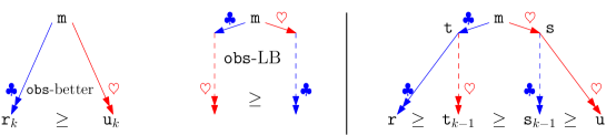
Figure 10. $\mathtt{obs}$-better

[$\mathtt{obs}$-better] The following properties are illustrated in Fig. 10.

• ${\color[rgb]{0,0,1}{{\color[rgb]{0,0,1}{\rightarrow_{\clubsuit}}}}}$ is $\mathtt{obs}$-better than ${\color[rgb]{1,0,0}{{\color[rgb]{1,0,0}{\rightarrow_{\heartsuit}}}}}$ ($\mathtt{obs}\mbox{-better}({\color[rgb]{0,0,1}{\rightarrow_{\clubsuit}}},{\color[rgb]{1,0,0}{{\color[rgb]{1,0,0}{\rightarrow_{\heartsuit}}}}})$): for each $\mathtt{m}$ and for each pair of a ${\color[rgb]{0,0,1}{{\color[rgb]{0,0,1}{\rightarrow_{\clubsuit}}}}}$-sequence $\langle\mathtt{r}_{n}\rangle_{n\in\mathbb{N}}$ and a ${\color[rgb]{1,0,0}{{\color[rgb]{1,0,0}{\rightarrow_{\heartsuit}}}}}$-sequence $\langle\mathtt{u}_{n}\rangle_{n\in\mathbb{N}}$ from $\mathtt{m}$, $\mathtt{obs}(\mathtt{r}_{n})\geq\mathtt{obs}(\mathtt{u}_{n})$ holds, for each $n$.

• ${\color[rgb]{0,0,1}{{\color[rgb]{0,0,1}{\rightarrow_{\clubsuit}}}}}$ is locally $\mathtt{obs}$-better than ${\color[rgb]{1,0,0}{{\color[rgb]{1,0,0}{\rightarrow_{\heartsuit}}}}}$ (written $\mathtt{obs}\mbox{-LB}({\color[rgb]{0,0,1}{\rightarrow_{\clubsuit}}},{\color[rgb]{1,0,0}{{\color[rgb]{1,0,0}{\rightarrow_{\heartsuit}}}}})$): if $\mathtt{t}{\color[rgb]{0,0,1}{~{}{}_{\clubsuit}\leftarrow}}\,{\mathtt{m}}\,{\color[rgb]{1,0,0}{{\color[rgb]{1,0,0}{\rightarrow_{\heartsuit}}}}}\mathtt{s}$, then for each $n\geq 0$, $\exists\mathtt{s}_{n},\mathtt{t}_{n}$, such that ${\color[rgb]{0,0,1}{\mathtt{s}\rightarrow_{\clubsuit}^{n}\mathtt{s}_{n}}}$, ${\color[rgb]{1,0,0}{\mathtt{t}{\color[rgb]{1,0,0}{\rightarrow_{\heartsuit}}}^{n}~{}\mathtt{t}_{n}}}$, and $\mathtt{obs}(\mathtt{t}_{n})\geq\mathtt{obs}(\mathtt{s}_{n})$

Remark 24.

Please notice that $\mathtt{obs}$-RD (resp. local $\mathtt{obs}$-RD) is a special case of $\mathtt{obs}\mbox{-better}$ (resp. $\mathtt{obs}\mbox{-LB}$). We have treated $\mathtt{obs}$-RD first and independently, for the sake of presentation.

It is immediate that $\mathtt{obs}\mbox{-better}({\color[rgb]{0,0,1}{{\color[rgb]{0,0,1}{\rightarrow_{\clubsuit}}}}},\rightarrow)$ implies that ${\color[rgb]{0,0,1}{{\color[rgb]{0,0,1}{\rightarrow_{\clubsuit}}}}}$ is $\mathtt{obs}$-complete for $\rightarrow$ (Def. 6.2). The notion of $\mathtt{obs}\mbox{-better}$ is again a condition which is expressive, but quantified over all reduction sequences from $\mathtt{m}$. We now prove that the local property $\mathtt{obs}\mbox{-LB}$ is sufficient to establish $\mathtt{obs}$-better, and even necessary when comparing with $\rightarrow$.

Theorem 25.

$\mathtt{obs}\mbox{-LB}({\color[rgb]{0,0,1}{{\color[rgb]{0,0,1}{\rightarrow_{\clubsuit}}}}},{\color[rgb]{1,0,0}{{\color[rgb]{1,0,0}{\rightarrow_{\heartsuit}}}}})$ implies $\mathtt{obs}\mbox{-better}({\color[rgb]{0,0,1}{{\color[rgb]{0,0,1}{\rightarrow_{\clubsuit}}}}},{\color[rgb]{1,0,0}{{\color[rgb]{1,0,0}{\rightarrow_{\heartsuit}}}}})$. The reverse also holds if either ${\color[rgb]{0,0,1}{{\color[rgb]{0,0,1}{\rightarrow_{\clubsuit}}}}}$ or ${\color[rgb]{1,0,0}{{\color[rgb]{1,0,0}{\rightarrow_{\heartsuit}}}}}$ is $\rightarrow$.

Proof 6.2.

$\boldsymbol{\Rightarrow}$. The proof is illustrated in Fig. 10. We prove by induction on $k$ the following:

$\mathtt{obs}\mbox{-LB}({\color[rgb]{0,0,1}{{\color[rgb]{0,0,1}{\rightarrow_{\clubsuit}}}}},{\color[rgb]{1,0,0}{{\color[rgb]{1,0,0}{\rightarrow_{\heartsuit}}}}})$ implies
$\big{(}\forall k,\forall\mathtt{m},\mathtt{r},\mathtt{u}\in C$, if ${\color[rgb]{0,0,1}{\mathtt{m}{\color[rgb]{0,0,1}{\rightarrow_{\clubsuit}}}^{k}\mathtt{r}}}$ and ${\color[rgb]{1,0,0}{\mathtt{m}{\color[rgb]{1,0,0}{\rightarrow_{\heartsuit}}}^{k}\mathtt{u}}}$, then $\mathtt{obs}(\mathtt{r})\geq\mathtt{obs}(\mathtt{u})\big{)}$ .

If $k=0$, the claim is trivial. If $k\geq 1$, let $\mathtt{m}{\color[rgb]{0,0,1}{\rightarrow_{\clubsuit}}}\mathtt{s}$ be the first step from $\mathtt{m}$ to $\mathtt{u}$, and $\mathtt{m}{\color[rgb]{1,0,0}{\rightarrow_{\heartsuit}}}\mathtt{t}$ the first step from $\mathtt{m}$ to $\mathtt{r}$, as in Fig. 10. $\mathtt{obs}\mbox{-LB}$ implies that there exist $\mathtt{s}_{k-1}$ and $\mathtt{t}_{k-1}$ such that ${\color[rgb]{0,0,1}{\mathtt{s}{\color[rgb]{0,0,1}{\rightarrow_{\clubsuit}}}^{k-1}\mathtt{s}_{k-1}}}$, ${\color[rgb]{1,0,0}{\mathtt{t}{\color[rgb]{1,0,0}{\rightarrow_{\heartsuit}}}^{k-1}~{}\mathtt{t}_{k-1}}}$, with $\mathtt{obs}(\mathtt{t}_{k-1})\geq\mathtt{obs}(\mathtt{s}_{k-1})$. Since ${\color[rgb]{1,0,0}{\mathtt{s}{\color[rgb]{1,0,0}{\rightarrow_{\heartsuit}}}^{k-1}~{}\mathtt{u}}}$ we can apply the induction hypothesis, and obtain that $\mathtt{obs}(\mathtt{s}_{k-1})\geq\mathtt{obs}(\mathtt{u})$. Again by induction hypothesis, from ${\color[rgb]{0,0,1}{\mathtt{t}{\color[rgb]{0,0,1}{\rightarrow_{\clubsuit}}}^{k-1}\mathtt{r}}}$ we obtain $\mathtt{obs}(\mathtt{r})\geq\mathtt{obs}(\mathtt{t}_{k-1})$. By transitivity, it holds that $\mathtt{obs}(\mathtt{r})\geq\mathtt{obs}(\mathtt{u})$.

$\boldsymbol{\Leftarrow}$. Assume ${\color[rgb]{1,0,0}{{\color[rgb]{1,0,0}{\rightarrow_{\heartsuit}}}}}=\rightarrow$, and $\mathtt{t}{\color[rgb]{0,0,1}{~{}{}_{\clubsuit}\leftarrow}}\mathtt{m}\rightarrow\mathtt{s}$. Let $\langle\mathtt{t}_{n}\rangle_{n\in\mathbb{N}}$ and $\langle\mathtt{s}_{n}\rangle_{n\in\mathbb{N}}$ be obtained by extending $\mathtt{t}$ and $\mathtt{s}$ with a maximal ${\color[rgb]{0,0,1}{{\color[rgb]{0,0,1}{\rightarrow_{\clubsuit}}}}}$ sequence. The claim follows from the hypothesis that ${\color[rgb]{0,0,1}{{\color[rgb]{0,0,1}{\rightarrow_{\clubsuit}}}}}$ dominates $\rightarrow$, by viewing the ${\color[rgb]{0,0,1}{{\color[rgb]{0,0,1}{\rightarrow_{\clubsuit}}}}}$ steps in $\langle\mathtt{s}_{n}\rangle_{n\in\mathbb{N}}$ as $\rightarrow$ steps.

Greatest Element.

Finally, we mention that $\mathtt{obs}\mbox{-LB}$ provides another method to establish $\mathtt{UN^{\mathtt{\infty}}}$, and therefore the fact that for each $\mathtt{m}$, $[\![\mathtt{m}]\!]$ is defined.

Proposition 26 (Greatest Element).

Given $\mathbf{Q}=\{(C,\rightarrow),\mathtt{obs}\}$, if there is a strategy ${\color[rgb]{0,0,1}{{\color[rgb]{0,0,1}{\rightarrow_{\clubsuit}}}}}$ such that $\mathtt{obs}\mbox{-LB}({\color[rgb]{0,0,1}{{\color[rgb]{0,0,1}{\rightarrow_{\clubsuit}}}}},\rightarrow)$, then $\mathbf{Q}$ satisfies $\mathtt{UN^{\mathtt{\infty}}}$.

Proof 6.3.

First, observe that the assumption implies in particular $\mathtt{obs}\mbox{-LB}({\color[rgb]{0,0,1}{{\color[rgb]{0,0,1}{\rightarrow_{\clubsuit}}}}},{\color[rgb]{0,0,1}{\rightarrow_{\clubsuit}}})$, and therefore (by Thm. 21) the QARS $((C,{\color[rgb]{0,0,1}{{\color[rgb]{0,0,1}{\rightarrow_{\clubsuit}}}}}),\mathtt{obs})$ satisfies $\mathtt{obs}$-RD. So, given $\mathtt{m}\in C$, all ${\color[rgb]{0,0,1}{\rightarrow_{\clubsuit}}}$-sequences from $\mathtt{m}$ have the same limit ${\bm{a}}$. From $\mathtt{obs}\mbox{-LB}({\color[rgb]{0,0,1}{{\color[rgb]{0,0,1}{\rightarrow_{\clubsuit}}}}},\rightarrow)$, it follows that ${\bm{a}}$ is the greatest limit of $\mathtt{Lim}_{\mathtt{obs}}(\mathtt{m})$.

7. PARS: Weighted Random Descent

When applied to PARS, $\mathtt{obs}$-RD is able to guarantee some remarkable properties: $\mathtt{UN^{\mathtt{\infty}}}$ and $p$-$\mathtt{SN^{\infty}}$ as soon as there exists a sequence which converges with probability $p$, and also the fact that all rewrite sequences from an element have the same expected number of steps.

Take $\mathtt{obs}$ to be either $-^{\scriptscriptstyle{\textsf{NF}}}$ or $\|-^{\scriptscriptstyle{\textsf{NF}}}\|$, $\mathtt{obs}$-RD implies that all rewrite sequences from $\mathtt{m}$:

• have the same probability of reaching a normal form after $k$ steps (for each $k\in\mathbb{N}$);

• converge to the same limit;

• have the same expected number of steps.

Proposition 27.

1. $\|-^{\scriptscriptstyle{\textsf{NF}}}\|$-RD implies $\mathtt{SN^{\infty}}$ (uniform normalization); moreover, for each $\mathtt{m}\in\mathsf{m}A$ all elements in $\mathtt{Lim}(\mathtt{m})$ are maximal.

2. $-^{\scriptscriptstyle{\textsf{NF}}}$-RD implies $\mathtt{SN^{\infty}}$ and $\mathtt{UN^{\mathtt{\infty}}}$.

Point-wise formulation.

In Section 7.2, we exploit the fact that not only $\mathtt{obs}$-RD  admits a local characterization, but also that the properties local $\mathtt{obs}$-RD and $\mathtt{obs}$-diamond can be expressed point-wise, making the condition even easier to verify.

1. pointed local $\mathtt{obs}$-RD: $\forall a\in A$, if $\mathtt{t}\leftleftarrows[a^{1}]\mathrel{\rightrightarrows}\mathtt{s}$, then $\forall k,\exists\mathtt{s}_{k},\mathtt{t}_{k}$ with $\mathtt{s}\mathrel{\rightrightarrows}^{k}\mathtt{s}_{k}$, $\mathtt{t}\mathrel{\rightrightarrows}^{k}\mathtt{t}_{k}$, and $\mathtt{obs}(\mathtt{s}_{k})=\mathtt{obs}(\mathtt{t}_{k})$.

2. pointed $\mathtt{obs}$-diamond: $\forall a\in A$, if $\mathtt{t}\leftleftarrows[a^{1}]\mathrel{\rightrightarrows}\mathtt{s}$, then it holds that $\mathtt{obs}(\mathtt{t})=\mathtt{obs}(\mathtt{s})$, and $\exists\mathtt{r}$ such that $\mathtt{t}\mathrel{\rightrightarrows}\mathtt{r}\leftleftarrows\mathtt{s}$.

Proposition 28 (point-wise local $\mathtt{obs}$-RD).

The following hold

• local $\mathtt{obs}$-RD iff pointed local $\mathtt{obs}$-RD;

• $\mathtt{obs}$-diamond iff pointed $\mathtt{obs}$-diamond.

Proof 7.1.

Immediate, by the definition of $\mathrel{\rightrightarrows}$. Given $\mathtt{m}=[p_{i}a_{i}]_{i\in I}$, we establish the result for each $a_{i}$, and put all the resulting multidistributions together.

7.1. Expected Termination Time

For ARS, Random Descent captures the property (Length) “all maximal rewrite sequences from an element have the same length.”

$\mathtt{obs}$-RD also implies a property similar to (Length) for PARS, where we consider not the number of steps of the rewrite sequences, but its probabilistic analogue, the expected number of steps.

In an ARS, if a maximal rewrite sequence terminates, the number of steps is finite; we interpret this number as time to termination. In the case of PARS, a system may have infinite runs even if it is AST; the number of rewrite steps $\rightarrow$ from an initial state is (in general) infinite. However, what interests us is its expected value, i.e.  the weighted average w.r.t. probability (see Section 2.2) which we write ETime($\langle\mathtt{m}_{n}\rangle_{n\in\mathbb{N}}$). This expected value can be finite; in this case, not only the system is AST, but is said PAST (Positively AST) (see [BG06]).

An example of probabilistic system with finite expected time to termination is the one in Fig. 3. The reduction from $c$ has ETime $2$. We can see this informally, recalling Section 2.2. Let the sample space $\Omega$ be the set of paths ending in a normal form, and let $\mu$ be the probability distribution on $\Omega$. What is the expected value of the random variable $\texttt{length}:\Omega\to\mathbb{N}$? We have $E(\texttt{length})=\sum_{\omega}\texttt{length}(\omega)\cdot\mu(\omega)=$ $\sum_{n\in\mathbb{N}}n\cdot\mu\{\omega\mid\texttt{length}(\omega)=n\}=$ $\sum n\cdot\frac{1}{2^{n}}=2$.

a very simple formulation, as follows:

$$\texttt{ETime}(\langle\mathtt{m}_{n}\rangle_{n\in\mathbb{N}})=\sum_{n\in\mathbb{N}}(1-\|\mathtt{m}_{n}^{\scriptscriptstyle{\textsf{NF}}}\|)$$ (1)

Intuitively, each tick in time (i.e. each $\mathrel{\rightrightarrows}$ step) is weighted with its probability to take place, which is $\mu_{i}\{c\mid c\not\in\scalebox{0.6}[1.0]{NF}_{\mathcal{A}}\}=1-\|\mathtt{m}_{i}^{\scriptscriptstyle{\textsf{NF}}}\|$ (where $\mu_{i}$ is the distribution over $A$ associated to $\mathtt{m}_{i}$). We refer to [ALY20] for the details.

It is immediate to check that in Example 5 (Fig. 3), the (unique) maximal rewrite sequence $\mathfrak{s}$ from $[c^{1}]$ has $\texttt{ETime}({\mathfrak{s}})=\sum_{n\in\mathbb{N}}\frac{1}{2^{n}}=2$.

Using this formulation, the following result is immediate.

Corollary 29.

Let $\mathtt{m}\in\mathsf{m}A$. $\|-^{\scriptscriptstyle{\textsf{NF}}}\|$-RD implies that all maximal rewrite sequences from $\mathtt{m}$ have the same ETime.

The well-known consequence is that $\sum_{n}(1-\|\mathtt{m}_{n}^{\scriptscriptstyle{\textsf{NF}}}\|)<\infty$ implies $\lim_{n\to\infty}(1-\|\mathtt{m}_{n}^{\scriptscriptstyle{\textsf{NF}}}\|)=0$, hence $\lim_{n\to\infty}\|\mathtt{m}_{n}^{\scriptscriptstyle{\textsf{NF}}}\|=1$. Cor. 29 means that if there exists one sequence from $\mathtt{m}$ with finite ETime, all do, hence $\mathtt{m}$ is AST and PAST .

7.2. Analysis of probabilistic reduction: Weak CbV $\lambda$-calculus

We define $\Lambda_{\oplus}^{\mathsf{w}}$, a probabilistic analogue of weak Call-by-Value $\lambda$-calculus (see Section 1.1.2). Evaluation is non-deterministic, because in the case of an application there is no fixed order in the evaluation of the left and right subterms (see Example 7.2.2). We show that $\Lambda_{\oplus}^{\mathsf{w}}$ satisfies $-^{\scriptscriptstyle{\textsf{NF}}}$-RD. Therefore it has remarkable properties (Cor. 31), analogous to those of its classical counter-part: the choice of the redex is irrelevant with respect to the final result, to its approximants, and to the expected number of steps.

7.2.1. The syntax

The set $\Lambda_{\oplus}$ of terms ($M,N,P,Q$) and the set $\mathcal{V}$ of values ($V,W$) are defined as follows:

$\begin{array}[]{lllc lll}M&{:}{:}{=}&x\mid\lambda x.M\mid MM\mid M\oplus M&&V&{:}{:}{=}&x\mid\lambda x.M\end{array}$

Free variables are defined as usual. A term $M$ is closed if it has no free variable. The substitution of $V$ for the free occurrences of $x$ in $M$ is denoted $M[x:=V]$.

pars.

The pars $(\Lambda_{\oplus},\rightarrow)$ is given by the set of terms together with the relation ${\rightarrow}\subseteq{\Lambda_{\oplus}\times\mathsf{Dst^{F}}(\Lambda_{\oplus})}$ which is inductively defined by the rules below.

$\begin{array}[]{l }(\lambda x.M)V\rightarrow\{M[x:=V]^{1}\}\\ P\oplus Q\rightarrow\{P^{1/2}\}+\{Q^{1/2}\}\\ \end{array}$

$\begin{array}[]{l }MN\rightarrow\{(MN_{i})^{p_{i}}\mid i\in I\}N\rightarrow\{N_{i}^{p_{i}}\mid i\in I\}\quad MN\rightarrow\{(M_{i}N)^{p_{i}}\mid i\in I\}M\rightarrow\{M_{i}^{p_{i}}\mid i\in I\}\end{array}$

PARS $\Lambda_{\oplus}^{\mathsf{w}}$.

The calculus $\Lambda_{\oplus}^{\mathsf{w}}$ is the PARS $(\mathsf{m}\Lambda_{\oplus},\mathrel{\rightrightarrows})$, where $\mathsf{m}\Lambda_{\oplus}$ is the set of multidistributions on $\Lambda_{\oplus}$, and ${\mathrel{\rightrightarrows}}\subseteq{\mathsf{m}\Lambda_{\oplus}\times\mathsf{m}\Lambda_{\oplus}}$ is the lifting (Definition 3.1) of $\rightarrow$.

7.2.2. Examples

[Non-deterministic evaluation]A term may have several reductions. The two reductions here join in one step: $\big{[}P[x:=Q](A\oplus B)\big{]}\leftleftarrows[((\lambda x.P)Q)(A\oplus B)]\rightrightarrows[\frac{1}{2}(\lambda x.P)QA,\frac{1}{2}(\lambda x.P)QB]$.

[Infinitary reduction] Let $R=(\lambda x.xx\oplus{\texttt{T}})(\lambda x.xx\oplus{\texttt{T}})$. We have $[R^{1}]\xRightarrow{\infty}\{{\texttt{T}}^{1}\}$. This term models the behaviour we discussed in Fig.3.

[Fix-Points] $\Lambda_{\oplus}^{\mathsf{w}}$ is expressive enough to allow fix-point combinators. A simple one is the Turing combinator $\Theta=AA$ where $A=\lambda xf.f(xxf)$. For each value $F$, $\{\Theta F\}\mathrel{\rightrightarrows}^{*}\{F(\Theta F)\}$.

The term $PR$ in Example 1.1.1 has (among others) the following reduction.

$$[PR] \mathrel{\rightrightarrows}[\frac{1}{2}P({\texttt{T}}\oplus{\texttt{F}}),\frac{1}{2}P(\Delta\Delta)]\mathrel{\rightrightarrows}[\frac{1}{4}P({\texttt{T}}),\frac{1}{4}P({\texttt{F}}),\frac{1}{2}P(\Delta\Delta)]$$

$$\mathrel{\rightrightarrows}^{*}[\frac{1}{4}({\texttt{T}}\mathtt{~{}XOR~{}}{\texttt{T}}),\frac{1}{4}({\texttt{F}}\mathtt{~{}XOR~{}}{\texttt{F}}),\frac{1}{4}\Delta\Delta]\mathrel{\rightrightarrows}[\frac{1}{4}{\texttt{F}},\frac{1}{4}{\texttt{F}},\frac{1}{2}\Delta\Delta]\dots$$

We conclude that $PR\xRightarrow{\infty}\{{\texttt{F}}^{1/2}\}$.

7.2.3. Properties

Theorem 30.

$\Lambda_{\oplus}^{\mathsf{w}}$ satisfies $\mathtt{obs}$-RD, with $\mathtt{obs}=-^{\scriptscriptstyle{\textsf{NF}}}$, because it satifies the $\mathtt{obs}$-diamond property.

Proof 7.2.

We prove the $\mathtt{obs}$-diamond property, using the definition of lifting and induction on the structure of the terms (see Appendix A.2).

Therefore, each $\mathtt{m}$ satisfies the following properties:

Corollary 31.

• All rewrite sequences from $\mathtt{m}$ converge to the same limit distribution.

• All rewrite sequences from $\mathtt{m}$ have the same expected termination time ETime.

• If $\mathtt{m}\mathrel{\rightrightarrows}^{k}\mathtt{s}$ and $\mathtt{m}\mathrel{\rightrightarrows}^{k}\mathtt{t}$, then $\mathtt{s}^{\scriptscriptstyle{\textsf{NF}}}=\mathtt{t}^{\scriptscriptstyle{\textsf{NF}}}$, $\forall\mathtt{s},\mathtt{t},k$.

7.3. More diamonds.

We have discussed weak evaluation of Call-by-Value $\lambda$-calculus, because this is arguably the most relevant paradigm for functional programming. Similar properties hold for several other reductions from the literature of $\lambda$-calculus, we just mention a few which are relevant to the probabilistic setting.

Call-by-Name $\lambda$-calculus has a non-deterministic variant of head reduction (well studied in Linear Logic) whose normal forms are precisely the head normal forms. Exactly as weak reduction for Call-by-Value, this variant is well known to satisfy the form of diamond which gives Random Descent. Another well-known calculus with a similar property is surface reduction in Simpson’s linear $\lambda$-calculus [Sim05]. For both—head CbN and surface reduction—Random Descent extends to the corresponding probabilistic reductions, which satisfy similar properties as those of $\Lambda_{\oplus}^{\mathsf{w}}$ (the proof is an easy variation of the one given here). All three reductions are used in [FR19].

Another calculus which satisfy Random Descent is Lafont’s interaction nets [Laf90]—we expect that its extension with a probabilistic choice would also satisfy Weighted Random Descent.

8. PARS: Comparing Strategies

In this section, we briefly examine the notion of $\mathtt{obs}\mbox{-better}$ in the setting of PARS. We focus on the following question:

“is there a strategy which is guaranteed to reach a normal form

with greatest probability”?

ARS Normalizing Strategies.

The strategy ${\mathrel{\mathop{\rightarrow}\limits_{\vbox to0.0pt{\kern-6.0pt\hbox{$\scriptstyle\textsc{s}~{}$}\vss}}}}\subseteq{\rightarrow}$ is a normalizing strategy for $\rightarrow$ if whenever $c\in A$ has a normal form, then every maximal $\mathrel{\mathop{\rightarrow}\limits_{\vbox to0.0pt{\kern-6.0pt\hbox{$\scriptstyle\textsc{s}~{}$}\vss}}}$-sequence from $c$ ends in a normal form.

PARS Normalizing Strategies.

Let $(\mathsf{m}A,\mathrel{\rightrightarrows})$ be a PARS. We recall that $\mathtt{Lim}_{\scriptscriptstyle{\|\|}}(\mathtt{m})=\{p\mid\mathtt{m}\xRightarrow{\infty}{}_{\mkern-12.0mu\scriptscriptstyle{\|\|}}p\}$. We write $q\geq\mathtt{Lim}_{\scriptscriptstyle{\|\|}}(\mathtt{m})$ if for each $p\in\mathtt{Lim}_{\scriptscriptstyle{\|\|}}(\mathtt{m})$, $q\geq p$. Similarly for $\leq$.

Given a PARS $(\mathsf{m}A,\mathrel{\rightrightarrows})$, a strategy ${{\color[rgb]{0,0,1}{\mathrel{\rightrightarrows}_{\clubsuit}}}}$ for $\mathrel{\rightrightarrows}$ is (asymptotically) normalizing if for each $\mathtt{m}$, each ${{\color[rgb]{0,0,1}{\mathrel{\rightrightarrows}_{\clubsuit}}}}$-sequence starting from $\mathtt{m}$ converges with the same probability $p_{\max}(\mathtt{m})\geq\mathtt{Lim}_{\scriptscriptstyle{\|\|}}(\mathtt{m})$. A strategy ${{\color[rgb]{1,0,0}{\mathrel{\rightrightarrows}_{\heartsuit}}}}$ for $\mathrel{\rightrightarrows}$ is (asymptotically) perpetual if for each $\mathtt{m}$, each ${{\color[rgb]{1,0,0}{\mathrel{\rightrightarrows}_{\heartsuit}}}}$ sequence from $\mathtt{m}$ converges with the same probability $p_{\min}(\mathtt{m})\leq\mathtt{Lim}_{\scriptscriptstyle{\|\|}}(\mathtt{m})$.

It is immediate that $\mathtt{obs}\mbox{-better}({\color[rgb]{0,0,1}{{\color[rgb]{0,0,1}{\mathrel{\rightrightarrows}_{\clubsuit}}}}},\mathrel{\rightrightarrows})$ with $\mathtt{obs}=\|-^{\scriptscriptstyle{\textsf{NF}}}\|$ implies that ${\color[rgb]{0,0,1}{{\color[rgb]{0,0,1}{\mathrel{\rightrightarrows}_{\clubsuit}}}}}$ is normalizing. By using the results in Section 6.3, we have a method to prove that a strategy is normalizing or perpetual by means of a local condition.

Corollary 32 (Normalizing criterion).

Let $\mathtt{obs}$ be $\|-^{\scriptscriptstyle{\textsf{NF}}}\|$. It holds that:

1. $\mathtt{obs}\mbox{-LB}({\color[rgb]{0,0,1}{{\color[rgb]{0,0,1}{\mathrel{\rightrightarrows}_{\clubsuit}}}}},{\mathrel{\rightrightarrows}})$ implies that ${\color[rgb]{0,0,1}{{\color[rgb]{0,0,1}{\mathrel{\rightrightarrows}_{\clubsuit}}}}}$ is asymptotically normalizing.

2. $\mathtt{obs}\mbox{-LB}(\mathrel{\rightrightarrows},{\color[rgb]{1,0,0}{{\color[rgb]{1,0,0}{\mathrel{\rightrightarrows}_{\heartsuit}}}}})$ implies that ${\color[rgb]{1,0,0}{{\color[rgb]{1,0,0}{\mathrel{\rightrightarrows}_{\heartsuit}}}}}$ is asymptotically perpetual.

Expected Number of Steps.

Let $\mathtt{obs}=\|-^{\scriptscriptstyle{\textsf{NF}}}\|$. Using Equation (1) in Section 7.1, it is easy to check that if $\mathtt{obs}$-better$({\color[rgb]{0,0,1}{{\color[rgb]{0,0,1}{\mathrel{\rightrightarrows}_{\clubsuit}}}}},\mathrel{\rightrightarrows})$ holds, and $\mathfrak{s}$ is a ${\color[rgb]{0,0,1}{{\color[rgb]{0,0,1}{\mathrel{\rightrightarrows}_{\clubsuit}}}}}$-sequence, then ETime($\mathfrak{s}$) $\leq$ETime($\mathfrak{t}$), for each $\mathfrak{t}$ $\mathrel{\rightrightarrows}$-sequence. Notice that $\mathtt{obs}$-better$({\color[rgb]{0,0,1}{{\color[rgb]{0,0,1}{\mathrel{\rightrightarrows}_{\clubsuit}}}}},\mathrel{\rightrightarrows})$ also implies that ETime($\mathfrak{s}$) is the same for any ${\color[rgb]{0,0,1}{{\color[rgb]{0,0,1}{\mathrel{\rightrightarrows}_{\clubsuit}}}}}$-sequence $\mathfrak{s}$. Therefore, to establish $\mathtt{obs}$-better$({\color[rgb]{0,0,1}{{\color[rgb]{0,0,1}{\mathrel{\rightrightarrows}_{\clubsuit}}}}},\mathrel{\rightrightarrows})$ implies not only that the strategy ${\color[rgb]{0,0,1}{{\color[rgb]{0,0,1}{\mathrel{\rightrightarrows}_{\clubsuit}}}}}$ is asymptotically normalizing, but also that it is of minimal expected termination time. A similar, dual observation holds for the perpetuity criterion.

9. Further work and discussion.

A larger example of application

Let us illustrate with an example the use of the tools which we have developed. We do so by summarizing further work [FR19]. There, for each of the following, Plotkin’s Call-by-Value [Plo75], Call-by-Name, and Simpson’s linear $\lambda$-calculus [Sim05], a fully fledged probabilistic extension is developed. Each probabilistic calculus satisfies confluence, and a form of standardization (surface standardization). To obtain confluence, only the probabilistic reduction is constrained, while $\beta$ reduction is unrestricted. In the three calculi, the role of asymptotically standard strategy is played by a reduction which is non-deterministic but satisfies Random Descent—this is necessary, because with the (usual) deterministic strategy, a standardization result for finite sequences fails.

Let us see some details.

The notion of result which is studied in [FR19] are, respectively, values in CbV, head normal forms in CbN, and surface normal forms in the linear calculus. Once confluence is established, [FR19] relies on the abstract results given in Section 5.4 to conclude that—in each calculus—the evaluation of a program $\mathtt{m}$ leads to a unique maximal result $[\![\mathtt{m}]\!]$—the greatest limit distribution. [FR19] then studies the question “is there a strategy which is guaranteed to reach the unique result (asymptotic standardization)?”. Again, key elements rely on the abstract tools developed here; let us sketch the construction.

We focus on the CbV calculus, namely $\Lambda_{\oplus}^{\mathtt{cbv}}=(\mathsf{m}\Lambda_{\oplus},\Rightarrow)$, where $\mathsf{m}\Lambda_{\oplus}$ is as in Section 7.2, and $\Rightarrow$ is the (more general) reduction which is defined in [FR19]. The role of standard strategy is played by a relation $\Rightarrow_{s}\subseteq\Rightarrow$ which is a (more relaxed) lifting of the weak reduction $\rightarrow$ defined in Section 7.2. The construction then goes as follows.

1. First, it is proved that $\Rightarrow_{s}$ is asymptotically complete for $\Rightarrow$. Note however that $\Rightarrow_{s}$ is not guaranteed to compute $[\![\mathtt{m}]\!]$.

2. It is observed that the relation $\mathrel{\rightrightarrows}$ as defined in Section 7.2 is asymptotically complete for $\Rightarrow_{s}$, and therefore for $\Rightarrow$.

3. The properties of $\mathrel{\rightrightarrows}$ which are proved in Section 7.2 guarantee that, from $\mathtt{m}$, the limit of any $\mathrel{\rightrightarrows}$-sequence is the same, and it is exactly $[\![\mathtt{m}]\!]$.

A similar reasoning applies to Call-by-Name.

Point 3. has another implication: for both CbN and CbV, the leftmost strategy reaches the best possible limit distribution (respectively over values and over head normal forms). This is remarkable for two reasons. First—as we already observed in Section 1.1.1—the leftmost strategy is the deterministic strategy which has been adopted in the literature of probabilistic $\lambda$-calculus, in either its CbV ([KMP97, DLMZ11]) or its CbN version ([DPHW05, EPT11]), but without any completeness result with respect to probabilistic computation. The work in [FR19] offers an “a-posteriori” justification for its use. Second, the result is non-trivial, because in the probabilistic case, a standardization result for finite sequences using the leftmost strategy fails for both CbV and CbN. The tools in Section 7 allow for an elegant solution.

On the necessity for non-deterministic evaluation and Random Descent in probabilistic $\lambda$-calculi

A programming language which is built on a $\lambda$-calculus implements a specific evaluation strategy. Typically, evaluation is given by a strategy $\mathrel{\mathop{\rightarrow}\limits_{\vbox to0.0pt{\kern-6.0pt\hbox{$\scriptstyle\textsc{s}~{}$}\vss}}}$ of the general reduction $\rightarrow$. In this paper, we studied a property of strategies which is more flexible than determinism, Random Descent. Why not simply fix a deterministic strategy? This choice has several motivations. Non-deterministic evaluation is a useful feature, which supports optimization techniques and parallel/distributed implementation, but in some cases it is also a necessity and a key reasoning tool—this appears clearly in the probabilistic case.

We illustrate this with two examples from the literature on probabilistic $\lambda$-calculus, [FR19] and [CP20]. Here we discuss the most familiar of all reductions: Call-by-Name $\lambda$-calculus with head reduction (similar arguments hold for weak reduction in CbV $\lambda$-calculus). The usual definition of head reduction [Bar84] is deterministic, but it also has a non-deterministic variant (well studied in Linear Logic) whose normal forms are precisely the head normal forms. We write this reduction simply $\mathrel{\mathop{\rightarrow}\limits_{\vbox to0.0pt{\kern-6.0pt\hbox{$\scriptstyle\mathsf{h}$}\vss}}}$. Exactly as weak reduction for Call-by-Value, $\mathrel{\mathop{\rightarrow}\limits_{\vbox to0.0pt{\kern-6.0pt\hbox{$\scriptstyle\mathsf{h}$}\vss}}}$ is well known to have Random Descent, and the same hold for its probabilistic incarnation (an explicit definition is in [FR19], Ch. X).

• In [FR19], moving from head reduction to its non-deterministic variant $\mathrel{\mathop{\rightarrow}\limits_{\vbox to0.0pt{\kern-6.0pt\hbox{$\scriptstyle\mathsf{h}$}\vss}}}$ allows to obtain a standardization result, which was known [Alb14, Lev19] not to hold when adopting usual, left-to-right head reduction (see [FR19], Ex. 45 for a counter-example).

• Similarly, Curzi and Pagani [CP20] move from usual head reduction to head spine reduction, which in turn is included in $\mathrel{\mathop{\rightarrow}\limits_{\vbox to0.0pt{\kern-6.0pt\hbox{$\scriptstyle\mathsf{h}$}\vss}}}$. The fact that the evaluation order is not left-to-right, but still there is no difference with respect to head normal forms is crucial to obtain the result of that paper.

10. Conclusions

The motivation behind this work is the need for theoretical tools to support the study of operational properties in probabilistic computation, similarly to the role that ARS have for classical computation.

We have investigated several abstract properties of probabilistic rewriting, and how the behaviour of different rewrite sequences starting from the same element compare w.r.t. normal forms. To guarantee that the result of a computation is well defined, we have introduced and studied the property $\mathtt{UN^{\mathtt{\infty}}}$, a robust probabilistic analogue of the notion of unique normal form. In particular, we have analyzed its relation with (various notions of) confluence. We also investigated relations with normalization ($\mathtt{WN^{\infty}}$) and termination ($\mathtt{SN^{\infty}}$), and between these notions. We have developed the notions of $\mathtt{obs}$-RD and $\mathtt{obs}\mbox{-better}$ as tools to analyze and compare PARS strategies. $\mathtt{obs}$-RD is an alternative to strict determinism, analogous to Random Descent for ARS (non-determinism is irrelevant w.r.t. a chosen event of interest). The notion of $\mathtt{obs}\mbox{-better}$ provides a sufficient criterion to establish that a strategy is normalizing (resp. perpetual) i.e. the strategy is guaranteed to lead to a result with maximal (resp. minimal) probability.

We have illustrated our techniques by studying a probabilistic extension of weak call-by-value $\lambda$-calculus; it has analogous properties to its classical counterpart: all rewrite sequences converge to the same result, in the same expected number of steps.

One-Step Reduction and Expectations.

In this paper, we focus on normal forms and properties related to the event $\scalebox{0.6}[1.0]{NF}_{\mathcal{A}}$. However, we believe that the methods would allow us to compare strategies w.r.t. other properties and random variables of the system. The formalism seems especially well suited to express the expected value of random variables. A key feature of the binary relation $\mathrel{\rightrightarrows}$ is to exactly capture the ARS notion of one-step reduction (in contrast to one or no step), with a gain which is two-folded.

1. Probability Theory. Because all terms in the distribution are forced to reduce at the same pace, a rewrite sequence faithfully represents the evolution in time of the system (i.e.   if $\mathtt{m}\mathrel{\rightrightarrows}^{i}\mathtt{m}_{i}$, then $\mathtt{m}_{i}$ captures the state at time $i$ of all possible paths $a_{0}\rightarrow\dots\rightarrow a_{i}$). This makes the formalism well suited to express the expected value of stochastic processes.

2. Rewrite Theory. The results in Sections 6.1, 6.3, 7.2, crucially rely on exactly one-step reduction. The reason why this is crucial, is similar to the classical fact that termination follows from normalization by the diamond property [Newman 1942], but not by the very similar property $b\leftarrow a\rightarrow c\Rightarrow\exists d~{}(b\rightarrow^{=}d~{}{}^{=}\leftarrow c$) (see [Terese], 1.3.18).

Finite Approximants.

$\mathtt{obs}$-RD characterizes the case when (not only at the limit, but also at the level of the approximants) the non-deterministic choices are irrelevant. The notion of approximant which we have studied here is “stop after a number $k$ of steps” ($k\in\mathbb{N}$). We can consider different notion of approximants. For example, we could also wish to stop the evolution of the system when it reaches a normal form with probability $p$. Our method can easily be adapted to analyze this case. We believe it is also possible to extend to the probabilistic setting the results in [vOT16], which would go further in this direction.

Further and future work.

In this paper, we have studied existence and uniqueness of the result of asymptotic computation. The next goal is to study how to compute such a result, i.e. the study of reduction strategies—this is the object of current investigation. [vO07] makes a convincing case of the power of the RD methods for ARS, by using a large range of examples from the literature, to elegantly and uniformly revisit normalization results of various $\lambda$-calculi. We cannot do the same here, because the rich development of strategies for $\lambda$-calculus has not yet an analogue in the probabilistic case. Nevertheless, we hope that the availability of tools to analyze PARS strategies will contribute to their development.

Acknowledgements.

This work benefited of fruitful discussions with U. Dal Lago, T. Leventis, and B. Valiron. I am very grateful to V. Van Oostrom for valuable comments and suggestions. The proof of Prop. 14 appearing here is a simplification of the original one, thanks to the insightful remarks of an anonymous reviewer.

Appendix A Omitted Proofs and Further Details

A.1. Section 5.2. Confluence and $\mathtt{UN^{\mathtt{\infty}}}$

Note that for ARS, UN does not imply confluence. Similarly, for QARS and PARS, $\mathtt{UN^{\mathtt{\infty}}}$ does not imply Confluence or Skew-Confluence. [$\mathtt{UN^{\mathtt{\infty}}}$ does not imply Confluence or Skew-Confluence] Consider the PARS generated by the following pars:

$c\to\{a^{\frac{1}{2}},{\texttt{F}}^{\frac{1}{2}}\}$, $c\to\{{\texttt{T}}^{\frac{1}{2}},b^{\frac{1}{2}}\}$, $a\to\{{\texttt{T}}^{\frac{1}{2}},a^{\frac{1}{2}}\}$, $b\to\{{\texttt{F}}^{\frac{1}{2}},b^{\frac{1}{2}}\}$.

Each PARS element $[c],[a],[b],\dots$ has a unique limit. No version of confluence holds, as it is easily seen taking the two sequences $[c]\mathrel{\rightrightarrows}[\frac{1}{2}a,\frac{1}{2}{\texttt{F}}]$ and $[c]\mathrel{\rightrightarrows}[\frac{1}{2}b,\frac{1}{2}{\texttt{T}}]$, and observing that they do not join, because there exists no $\mathtt{m}$ such that $[\frac{1}{2}a,\frac{1}{2}{\texttt{F}}]\mathrel{\rightrightarrows}^{*}\mathtt{m}$ and $[\frac{1}{2}b,\frac{1}{2}{\texttt{T}}]\mathrel{\rightrightarrows}^{*}\mathtt{m}$

Remark 33 (QARS limits vs ARSI infinite normal forms).

The notion of limit which is associated to QARS is more general than the notion of infinite normal form which is defined for ARSI [AB02]. Note that in the setting of [AB02] the following holds (Theorem 5.4 there):

“an ARSI is skew confluent if and only if it has unique infinite normal forms”.

An analogue property does not hold for QARS. Even for PARS, the “if” direction fails (Ex. A.1).

A.2. Section 7.2. Weak CbV $\lambda$-calculus

Theorem (30).

$\Lambda_{\oplus}^{\mathsf{w}}$ satisfies the $\mathtt{obs}$-diamond property, with $\mathtt{obs}=-^{\scriptscriptstyle{\textsf{NF}}}$.

Proof A.1.

We show by induction on the structure of the term $M$ that for all pairs of one-step reductions $\mathtt{t}\leftleftarrows[M^{1}]\mathrel{\rightrightarrows}\mathtt{s}$, either $\mathtt{t}=\mathtt{s}$, (and therefore $\exists\mathtt{u}.~{}\mathtt{t}\mathrel{\rightrightarrows}\mathtt{u}\leftleftarrows\mathtt{s}$) or the following hold: (1.) $\mathtt{s}^{\scriptscriptstyle{\textsf{NF}}}=\bm{0}=\mathtt{t}^{\scriptscriptstyle{\textsf{NF}}}$ (i.e. they are equal because they both take value $0$ everywhere), and (2.) exists $\mathtt{u}$ such that $\mathtt{t}\mathrel{\rightrightarrows}\mathtt{u}\leftleftarrows\mathtt{s}$.

• Case $M=x$ or $M=\lambda x.P$: no reduction is possible.

• Case $M=P\oplus Q$, or $M=(\lambda x.N)V$: only one reduction is possible, and $\mathtt{t}=\mathtt{s}$.

• Otherwise, $M=PQ$, and two cases are possible.

  • Assume that both $P$ and $Q$ reduce; $PQ$ has the following reductions:

    $PQ\rightarrow\{(P_{i}Q)^{p_{i}}\mid i\in I\}P\rightarrow\{(P_{i})^{p_{i}}\mid i\in I\}$  and  $PQ\rightarrow\{(PQ_{j})^{q_{j}}\mid j\in J\}Q\rightarrow\{Q_{j}^{q_{j}}\mid j\in J\}$

    Observe that none of the $P_{i}Q$ or $PQ_{j}$ is a normal form, hence (1.) holds. By the definition of $\rightarrow$, the following holds

    $\left(P_{i}Q\rightarrow\{(P_{i}Q_{j})^{q_{j}}\mid j\in J\}Q\rightarrow\{Q_{j}^{q_{j}}\mid j\in J\}\right)_{i\in I}$

    and therefore by Lifting we have $\sum_{i}p_{i}\cdot[P_{i}Q]\mathrel{\rightrightarrows}\sum_{i}p_{i}\cdot(\sum_{j}q_{j}\cdot[P_{i}Q_{j}])=\sum_{i,j}p_{i}q_{j}\cdot[P_{i}Q_{j}]$. Similarly we obtain $\sum_{j}q_{j}\cdot[PQ_{j}]\mathrel{\rightrightarrows}\sum_{i,j}p_{i}q_{j}\cdot[P_{i}Q_{j}]$.

  • If one subterm has two reductions, we conclude by i.h..

    Let assume that $P$ has two different redexes (the case of $Q$ is similar):

    $[P]\mathrel{\rightrightarrows}\mathtt{s}=\sum_{i}s_{i}\cdot[S_{i}]$ and $[P]\mathrel{\rightrightarrows}\mathtt{t}=\sum_{j}t_{j}\cdot[T_{j}]$

    By induction hypothesis, two facts hold: (1.) $\mathtt{s}^{\scriptscriptstyle{\textsf{NF}}}=\bm{0}=\mathtt{t}^{\scriptscriptstyle{\textsf{NF}}}$, therefore no $S_{i}$ and no $T_{j}$ is a normal form; (2.) there exist steps $[S_{i}]\mathrel{\rightrightarrows}\sum_{k}r_{k}\cdot[R_{ik}]$ and $[T_{j}]\mathrel{\rightrightarrows}r_{h}\cdot[R_{jh}]$ such that $P\mathrel{\rightrightarrows}\sum_{i}[S_{i}]\mathrel{\rightrightarrows}\sum_{i}(\sum_{k}s_{i}r_{k}\cdot[R_{ik}])=\mathtt{r}^{\prime}$ and $P\mathrel{\rightrightarrows}\sum_{j}[T_{j}]\mathrel{\rightrightarrows}\sum_{j}(\sum_{h}t_{j}r_{h}\cdot[R_{jh}])=\mathtt{r}^{\prime\prime}$, and $\mathtt{r}^{\prime}=\mathtt{r}^{\prime\prime}$.

    For $PQ$ we have

    $PQ\rightarrow\{(S_{i}Q)^{s_{i}}\mid i\in I\}P\rightarrow\{S_{i}^{s_{i}}\mid i\in I\}$ and  $PQ\rightarrow\{(T_{j}Q)^{t_{j}}~{}\mid~{}j\in J\}P\rightarrow\{T_{j}^{t_{j}}~{}\mid~{}j\in J\}$

    First, we observe that no $S_{i}Q$ and no $T_{j}Q$ is a normal form, hence property (1.) is verified. Moreover, it holds that

    $PQ\mathrel{\rightrightarrows}\sum_{i}s_{i}\cdot[S_{i}Q]\mathrel{\rightrightarrows}\sum_{i}(\sum_{k}s_{i}r_{k}\cdot[R_{ik}Q])=\mathtt{u}^{\prime}$ and $PQ\mathrel{\rightrightarrows}\sum_{j}t_{j}\cdot[T_{j}Q]\mathrel{\rightrightarrows}\sum_{j}(\sum_{h}t_{j}r_{h}\cdot[R_{jh}Q])=\mathtt{u}^{\prime\prime}$. From $\mathtt{r}^{\prime}=\mathtt{r}^{\prime\prime}$ it follows that $\mathtt{u}^{\prime}=\mathtt{u}^{\prime\prime}$; hence property (2.) is also verified.

References

- [AB02] Zena M. Ariola and Stefan Blom. Skew confluence and the lambda calculus with letrec. Annals of Pure and Applied Logic, 117(1):95 – 168, 2002.
- [AC98] Roberto M. Amadio and Pierre-Louis Curien. Domains and lambda-calculi, volume 46 of Cambridge tracts in theoretical computer science. Cambridge University Press, 1998.
- [ACN18] Sheshansh Agrawal, Krishnendu Chatterjee, and Petr Novotný. Lexicographic ranking supermartingales: an efficient approach to termination of probabilistic programs. PACMPL, 2(POPL):34:1–34:32, 2018.
- [Alb14] Michele Alberti. On operational properties of quantitative extensions of -calculus. PhD thesis, Aix-Marseille University, France, 2014.
- [ALY20] Martin Avanzini, Ugo Dal Lago, and Akihisa Yamada. On probabilistic term rewriting. Sci. Comput. Program., 185, 2020.
- [AMS06] Gul A. Agha, José Meseguer, and Koushik Sen. PMaude: Rewrite-based specification language for probabilistic object systems. Electr. Notes Theor. Comput. Sci., 153(2):213–239, 2006.
- [Bar84] Hendrik Pieter Barendregt. The Lambda Calculus – Its Syntax and Semantics, volume 103 of Studies in logic and the foundations of mathematics. North-Holland, 1984.
- [BG06] Olivier Bournez and Florent Garnier. Proving positive almost sure termination under strategies. In Rewriting Techniques and Applications, RTA, pages 357–371, 2006.
- [BK02] Olivier Bournez and Claude Kirchner. Probabilistic rewrite strategies. Applications to ELAN. In Rewriting Techniques and Applications, RTA, pages 252–266, 2002.
- [CH98] N. Cagman and J.R. Hindley. Combinatory weak reduction in lambda calculus. Theor. Comput. Sci., 1998.
- [CP20] Gianluca Curzi and Michele Pagani. The benefit of being non-lazy in probabilistic -calculus: Applicative bisimulation is fully abstract for non-lazy probabilistic call-by-name. In LICS ’20: 35th Annual ACM/IEEE Symposium on Logic in Computer Science, 2020, pages 327–340. ACM, 2020.
- [DAGG11] Alejandro Díaz-Caro, Pablo Arrighi, Manuel Gadella, and Jonathan Grattage. Measurements and confluence in quantum lambda calculi with explicit qubits. Electr. Notes Theor. Comput. Sci., 270(1):59–74, 2011.
- [DKP91] Nachum Dershowitz, Stéphane Kaplan, and David A. Plaisted. Rewrite, rewrite, rewrite, rewrite, rewrite, … Theor. Comput. Sci., 83(1):71–96, 1991.
- [DLM08] Ugo Dal Lago and Simone Martini. The weak lambda calculus as a reasonable machine. Theor. Comput. Sci., 398(1-3):32–50, 2008.
- [DLMZ11] Ugo Dal Lago, Andrea Masini, and Margherita Zorzi. Confluence results for a quantum lambda calculus with measurements. Electr. Notes Theor. Comput. Sci., 270(2):251–261, 2011.
- [DLZ12] Ugo Dal Lago and Margherita Zorzi. Probabilistic operational semantics for the lambda calculus. RAIRO - Theor. Inf. and Applic., 46(3):413–450, 2012.
- [DM18] Alejandro Díaz-Caro and Guido Martinez. Confluence in probabilistic rewriting. Electr. Notes Theor. Comput. Sci., 338:115–131, 2018.
- [dP95] Ugo de’Liguoro and Adolfo Piperno. Non deterministic extensions of untyped lambda-calculus. Inf. Comput., 122(2):149–177, 1995.
- [DPHW05] Alessandra Di Pierro, Chris Hankin, and Herbert Wiklicky. Probabilistic lambda-calculus and quantitative program analysis. J. Log. Comput., 15(2):159–179, 2005.
- [EPT11] Thomas Ehrhard, Michele Pagani, and Christine Tasson. The computational meaning of probabilistic coherence spaces. In Proceedings of the 26th Annual IEEE Symposium on Logic in Computer Science, LICS 2011, pages 87–96. IEEE Computer Society, 2011.
- [Fag19] Claudia Faggian. Probabilistic rewriting: Normalization, termination, and unique normal forms. In 4th International Conference on Formal Structures for Computation and Deduction, FSCD 2019, volume 131 of LIPIcs, pages 19:1–19:25. Schloss Dagstuhl, 2019.
- [FC19] Hongfei Fu and Krishnendu Chatterjee. Termination of nondeterministic probabilistic programs. In Verification, Model Checking, and Abstract Interpretation VMCAI, pages 468–490, 2019.
- [FH15] Luis María Ferrer Fioriti and Holger Hermanns. Probabilistic termination: Soundness, completeness, and compositionality. In POPL, pages 489–501, 2015.
- [FR19] Claudia Faggian and Simona Ronchi Della Rocca. Lambda calculus and probabilistic computation. In 34th Annual ACM/IEEE Symposium on Logic in Computer Science, LICS 2019, pages 1–13. IEEE, 2019.
- [HFCG19] Mingzhang Huang, Hongfei Fu, Krishnendu Chatterjee, and Amir Kafshdar Goharshady. Modular verification for almost-sure termination of probabilistic programs. Proc. ACM Program. Lang., 3(OOPSLA):129:1–129:29, 2019.
- [How70] W.A. Howard. Assignment of ordinals to terms for primitive recursive functionals of finite type. In Intuitionism and Proof Theory, 1970.
- [KC17] Maja H. Kirkeby and Henning Christiansen. Confluence and convergence in probabilistically terminating reduction systems. In Logic-Based Program Synthesis and Transformation - 27th International Symposium, LOPSTR 2017, pages 164–179, 2017.
- [KdV05] Jan Willem Klop and Roel C. de Vrijer. Infinitary normalization. In We Will Show Them! Essays in Honour of Dov Gabbay, Volume Two, pages 169–192, 2005.
- [Ken92] Richard Kennaway. On transfinite abstract reduction systems. Tech. rep., CWI, Amsterdam, 1992.
- [KKMO18] Benjamin Lucien Kaminski, Joost-Pieter Katoen, Christoph Matheja, and Federico Olmedo. Weakest precondition reasoning for expected runtimes of randomized algorithms. J. ACM, 65(5):30:1–30:68, 2018.
- [KKSdV95] Richard Kennaway, Jan Willem Klop, M. Ronan Sleep, and Fer-Jan de Vries. Transfinite reductions in orthogonal term rewriting systems. Inf. Comput., 119(1):18–38, 1995.
- [KMP97] Daphne Koller, David A. McAllester, and Avi Pfeffer. Effective bayesian inference for stochastic programs. In National Conference on Artificial Intelligence and Innovative Applications of Artificial Intelligence Conference, AAAI 97, IAAI 97, pages 740–747, 1997.
- [Laf90] Yves Lafont. Interaction nets. In Conference Record of the Seventeenth Annual ACM Symposium on Principles of Programming Languages, San Francisco, California, USA, January 1990, pages 95–108. ACM Press, 1990.
- [Ler90] Xavier Leroy. The ZINC experiment: an economical implementation of the ML language. Technical report 117, INRIA, 1990. URL: http://gallium.inria.fr/~xleroy/publi/ZINC.pdf.
- [Lév78] Jean-Jacques Lévy. Réductions Corrects et Optimales dans le Lambda-Calcul. PhD thesis, Université Paris VII, 1978.
- [Lev19] Thomas Leventis. A deterministic rewrite system for the probabilistic -calculus. Mathematical Structures in Computer Science, 29(10):1479–1512, 2019.
- [LFR21] Ugo Dal Lago, Claudia Faggian, and Simona Ronchi Della Rocca. Intersection types and (positive) almost-sure termination. Proc. ACM Program. Lang., 5(POPL):1–32, 2021.
- [LFVY17] Ugo Dal Lago, Claudia Faggian, Benoît Valiron, and Akira Yoshimizu. The geometry of parallelism: classical, probabilistic, and quantum effects. In Proceedings of the 44th ACM SIGPLAN Symposium on Principles of Programming Languages, POPL 2017, Paris, pages 833–845. ACM, 2017.
- [Mar13] Simon Marlow. Parallel and Concurrent Programming in Haskell. O’Reilly Media, 2013.
- [MMKK18] Annabelle McIver, Carroll Morgan, Benjamin Lucien Kaminski, and Joost-Pieter Katoen. A new proof rule for almost-sure termination. PACMPL, 2(POPL):33:1–33:28, 2018.
- [New42] Mark Newman. On theories with a combinatorial definition of “Equivalence”. Annals of Mathematics, 43(2):223–243, 1942.
- [Plo75] Gordon D. Plotkin. Call-by-name, call-by-value and the lambda-calculus. Theor. Comput. Sci., 1(2):125–159, 1975.
- [PPT05] Sungwoo Park, Frank Pfenning, and Sebastian Thrun. A probabilistic language based upon sampling functions. In Proceedings of the 32nd ACM SIGPLAN-SIGACT Symposium on Principles of Programming Languages, POPL 2005, pages 171–182. ACM, 2005.
- [Put94] Martin L. Puterman. Markov Decision Processes: Discrete Stochastic Dynamic Programming. John Wiley & Sons, Inc., New York, NY, USA, 1st edition, 1994.
- [Rab63] Michael O. Rabin. Probabilistic automata. Information and Control, 6(3):230–245, 1963.
- [RP02] Norman Ramsey and Avi Pfeffer. Stochastic lambda calculus and monads of probability distributions. In Conference Record of POPL 2002: The 29th SIGPLAN-SIGACT Symposium on Principles of Programming Languages, 2002, pages 154–165. ACM, 2002.
- [Sah78] N. Saheb-Djahromi. Probabilistic LCF. In Mathematical Foundations of Computer Science, pages 442–451, 1978.
- [San71] Eugene S. Santos. Computability by probabilistic turing machines. In Transactions of the American Mathematical Society, pages 159:165–184, 1971.
- [Sim05] Alex K. Simpson. Reduction in a linear lambda-calculus with applications to operational semantics. In Rewriting Techniques and Applications, RTA, pages 219–234, 2005.
- [Ter03] Terese. Term Rewriting Systems, volume 55 of Cambridge Tracts in Theoretical Computer Science. Cambridge University Press, 2003.
- [vO07] Vincent van Oostrom. Random descent. In Term Rewriting and Applications, RTA, page 314–328, 2007.
- [vOT16] Vincent van Oostrom and Yoshihito Toyama. Normalisation by random descent. In Formal Structures for Computation and Deduction, FSCD, pages 32:1–32:18, 2016.