Abstract: This article illustrates how to measure the heterogeneity of spatial data presenting a finite number of categories via computation of spatial entropy. The R package SpatEntropy contains functions for the computation of entropy and spatial entropy measures. The extension to spatial entropy measures is a unique feature of SpatEntropy. In addition to the traditional version of Shannon’s entropy, the package includes Batty’s spatial entropy, O’Neill’s entropy, Li and Reynolds’ contagion index, Karlstrom and Ceccato’s entropy, Leibovici’s entropy, Parresol and Edwards’ entropy and Altieri’s entropy. The package is able to work with both areal and point data.

This paper is a general description of SpatEntropy, as well as its necessary theoretical background, and an introduction for new users.

Keywords: Spatial entropy, Shannon’s entropy, entropy decomposition, spatial data heterogeneity, categorical variables

1 Introduction: entropy and spatial entropy in R

SpatEntropy is the first R package allowing to compute entropy measures for spatial data. In applied sciences, data heterogeneity is often evaluated via computation of entropy. Entropy (Shannon, 1948) comes from Information Theory (Cover and Thomas, 2006), but is often employed in many statistical contexts because of its ability to synthesize different concepts such as information, surprise, uncertainty, heterogeneity, contagion; moreover, entropy indices can be constructed on any kind of variables, even unordered qualitative ones, since the computation only involves the probability of occurrence of each category. For these reasons, fields such as geography, ecology, biology and landscape studies usually refer to entropy for data description and interpretation (Frosini, 2004). Often, these disciplines deal with spatial data, i.e., data that are georeferenced as points or areas. In such contexts, entropy measures should include spatial information; therefore, a number of works are available in the literature, aiming at building a spatial entropy index. They can be ascribed to three main approaches. The first starts with Batty (1974, 1976, 2010) who defines a spatial entropy measure which evaluates the distribution of an event over an area, allowing for unequal space partition into sub-areas. Later, Karlström and Ceccato (2002) modified the initial proposal in order to satisfy the property of additivity in terms of decomposition of the global index into local components, following LISA criteria (Anselin, 1995). The second approach to spatial entropy includes space based on a suitable transformation of the study variable to account for the distance between realizations (co-occurrences); the first proposal is made by O’Neill et al. (1988) for contiguous couples of realizations, extended by Leibovici (2009) and Leibovici et al. (2014) to further distances and general degrees of co-occurrences. Contagion indices (Li and Reynolds, 1993; Parresol and Edwards, 2014) are also based on this view: spatial contagion is the opposite of entropy. As for the third approach, a set of spatial entropy measures has been presented by Altieri et al. (2018a), starting from the co-occurrence approach but overcoming some undesirable features of the previous measures. According to this framework, Shannon’s entropy of the transformed variable is decomposed into the information due to space and the remaining information brought by the transformed variable once space is considered. The proposal solves the problem of preserving additivity and disaggregating results, allowing for partial and global syntheses.

In R (R Core Team, 2017), the main available packages for standard entropy measures are entropart, entropy and EntropyEstimation. They allow basic entropy computation and decomposition into its two terms mutual information and conditional entropy (Cover and Thomas, 2006). A quick comparison to these packages is in Section 2. There was no package available for spatial entropy measures, which translates the above concept into a spatial context. This work illustrates how to make use of the new package SpatEntropy (Altieri et al., 2018b), which collects functions for all the spatial entropy indices mentioned above. SpatEntropy makes extensive use of spatstat functions and data structures (Baddeley et al., 2015). The package is built in such a way that it can be used by non-statisticians, provided they have basic knowledge of R; the minimum effort is requested to the user.

The following Section introduces basic notions regarding Shannon’s entropy and the data examples used throughout the paper. Then, the article is organized into three Sections for the three main branches of spatial entropy measures: Section 3 refers to Batty’s approach; Section 4 gives details for O’Neill’s approach; Section 5 illustrates Altieri’s approach. Each Section can be read independently: it starts with the essential theoretical background, and then guides the reader through worked out examples covering both areal and point datasets.

2 Data examples and entropy basics

Two datasets are used for illustration along the paper, both available within SpatEntropy.

The areal dataset data_bologna comes from the EU CORINE Land Cover project (EEA, 2011) dated 2011. It classifies the original land cover data into urbanised and non-urbanised zones, known as ’Urban Morphological Zones’ (UMZ). UMZ data are useful to identify shapes and patterns of urban areas, and thus to detect what is known as urban sprawl (Altieri et al., 2014). Bologna’s metropolitan area is extracted from the European CORINE dataset and is composed by the municipality of Bologna and the surrounding municipalities. The dataset is made of $120\times 96$ pixels of size $250\times 250$ metres and is shown in Figure 1, where a black pixel is urban and a white pixel is non-urban. In order to speed up the results for the examples, the present paper uses a trimmed version of the original dataset: boData, with $n=50\times 50=2500$ cells.

R> boData=data_bologna[41:90, 26:75]
R> plot_lattice(boData, ribbon=F)

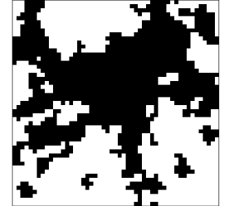
Figure 1: Trimmed Bologna urban data.

The SpatEntropy function plot_lattice allows to easily produce a gray scale map given a matrix of categorical data and, optionally, the observation area. It ensures that data is displayed following the matrix order (where position [1,1] corresponds to the top-left corner of the plot), avoiding risks of row inversion or transposition. A few options may be tuned, such as the extent of the gray scale, the title and the colour side legend.

The second example dataset is data_rainforest, a marked point pattern dataset about four rainforest tree species. This dataset documents the presence of tree species over Barro Colorado Island, Panama. Barro Colorado Island has been the focus of intensive research on lowland tropical rainforest since 1923 (http://www.ctfs.si.edu). Research identified several tree species over a rectangular observation window of size $1000\times 500$ metres; the tree species constitute the point data categorical mark. This dataset presents 4 species with different spatial configurations: Acalypha diversifolia, Chamguava schippii, Inga pezizifera and Rinorea sylvatica. The overall dataset has a total number of 7251 points. The dataset is analyzed with spatial entropy measures in (Altieri et al., 2018a). In the present article, we propose a trimmed version of the rainforest tree dataset: treeData with $n=1982$ trees, shown in Figure 2.

R> smallW=owin(xrange=c(350,800), yrange=c(300,500))
R> treeData=data_rainforest[smallW]
R> plot.ppp(treeData, cols=1:4, pch=19)

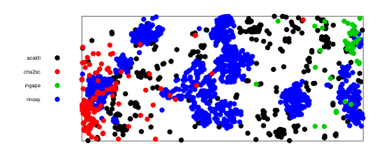
Figure 2: Trimmed rainforest tree data.

The function owin belongs to spatstat and builds an observation area of fixed size, that we use for selecting a subset of the dataset. The function plot.im also comes from spatstat and is needed for plotting a point pattern object (an object of class ppp).

As a starting illustrative point, we compute Shannon’s entropy for the two datasets. Let $X$ be a discrete random variable taking values $x_{i}$ in a set of $I$ outcomes. In the first above example $X$ classifies soil in $x_{1}$ ’urban’ and $x_{2}$ ’non-urban’ for Bologna, while for the rainforest trees $X$ is the tree species with $I=4$ categories $x_{1}$ to $x_{4}$. Let $p_{X}=(p(x_{1}),\dots,p(x_{I}))^{\prime}$ be the probability mass function (pmf) of $X$. Shannon’s entropy of $X$ is defined as

$$H(X)=\sum_{i=1}^{I}p(x_{i})\log\left(\frac{1}{p(x_{i})}\right).$$ (1)

Entropy quantifies the average amount of information brought by $X$ according to the pmf $p_{X}$; it is the expected value of the information function $I(p_{X})$, where $I(p(x_{i}))=\log(1/p(x_{i}))$. Intuitively, outcomes with a very low probability of occurrence increase the entropy value, while outcomes very likely to occur give a small contribution to entropy. Thus, entropy measures the information coming from observing realizations, or, in other words, the surprise, which is larger when outcomes are observed that are not likely to occur. Entropy ranges in $[0,\log(I)]$ and its maximum value is achieved when $X$ is uniformly distributed.

In SpatEntropy, Shannon’s entropy can be computed for a dataset with shannonX, a function which takes matrices or vectors of any type as inputs, and returns estimated probabilities (frequencies) for all data categories together with Shannon’s entropy of the dataset.

R> shan.bo=shannonX(boData)

$probabilities
category frequency
1 0 0.5178777
2 1 0.4821223

$shannon
[1] 0.6925078

If the dataset is a ppp object such as treeData, the input of shannonX is the vector of point marks, i.e., the vector with the tree species.

R> shan.tree=shannonX(marks(treeData))

$probabilities
category frequency
1 acaldi 0.19374369
2 cha2sc 0.06205853
3 ingape 0.02320888
4 rinosy 0.72098890

$shannon
[1] 0.8136769

In many situations, entropy is seen as a descriptive measure. It can also be seen as an estimator $\widehat{H}(X)$, where the probability distribution is estimated by the so-called plug-in estimator (Paninski, 2003), which is the nonparametric as well as the maximum likelihood estimator: $\widehat{p}(x_{i})=n_{i}/n$ substitutes the probabilities with the observed proportions over $n$ realizations. Such estimator has known properties (Paninski, 2003), and its variance is

$$V[\widehat{H}(X)]=V[I(p_{X})]=\widehat{H}(X)^{(2)}-(\widehat{H}(X))^{2},$$ (2)

where $H(X)^{(2)}=\sum_{i=1}^{I}p(x_{i})\log\left(\frac{1}{p(x_{i})}\right)^{2}$. For computing such variance, a useful function is available, shannonX_sq, which computes $\widehat{H}(X)^{(2)}$:

R> shan.bo2=shannonX_sq(boData)
R> Vshan.bo=shan.bo2$shannon.square-(shan.bo$shannon^2)
R> Vshan.bo

[1] 0.001277909

R> shan.tree2=shannonX_sq(marks(treeData))
R> Vshan.tree=shan.tree2$shannon.square-(shan.tree$shannon^2)
R> Vshan.tree

[1] 0.7451366

The variance of entropy, seen as an estimator, is small when the dataset is large.

Shannon’s entropy can also be computed with the packages entropart, entropy and Entropy
Estimation. Using the Bologna data example, the function Shannon of entropart and the function entropy.plugin of entropy return the same value for $H(X)=0.6925078$, but they are less user-friendly since they require the estimates for the probabilities of all $X$ categories, while shannonX relies on raw data. The package EntropyEstimation cannot be used for comparison since it only computes the class of entropy estimators proposed by Zhang (2012).

A major drawback of Shannon’s entropy is that it does not account for the spatial location of occurrences, so that datasets with identical (estimated) pmf but very different spatial configurations share the same entropy value. The following Sections present, both in theory and practice, the three main approaches to building spatial entropy measures. Most of these measures imply the formal definition of a neighbourhood (Cressie, 1993). The simplest way of representing a neighbourhood system over $n$ spatial units is via an adjacency matrix (Anselin, 1995), i.e., a square matrix whose elements indicate whether pairs of units are neighbours: $a_{uu^{\prime}}=1$ if $u^{\prime}\in\mathcal{N}(u)$, that is the neighbourhood of area $u$; $a_{uu}=0$ by definition. Spatial units may be points, defined via coordinate pairs, or areas, identified via representative coordinate pairs, such as the area centroids.

3 Spatial entropy for an area partition

Batty’s spatial entropy (Batty, 1974, 1976, 2010) is useful for evaluating the heterogeneity in the distribution of a phenomenon over an area. It is particularly appropriate when the observation area is exogenously partitioned into sub-areas (such as municipality administrative boundaries for a Region). If the probabilities of the neighbouring sub-areas should enter the computation, one should resort to the proposal by Karlström and Ceccato (2002).

3.1 Batty’s entropy

Let a phenomenon of interest $F$ occur over an observation window of size $T$ partitioned into $G$ areas of size $T_{g}$. This defines $G$ dummy variables identifying the occurrence of $F$ over a generic area $g$, $g=1,\dots,G$. Given that $F$ occurs over the window, its occurrence in area $g$ takes place with probability $p_{g}$, where $1-p_{g}=\sum_{g^{\prime}\neq g}p_{g^{\prime}}$ and $\sum_{g}p_{g}=1$. The phenomenon intensity is obtained as $\lambda_{g}=p_{g}/T_{g}$, where $T_{g}$ is the area size, and is assumed constant within each area. Batty’s spatial entropy is

$$H_{B}(F)=\sum_{g=1}^{G}p_{g}\log\left(\frac{T_{g}}{p_{g}}\right).$$ (3)

It expresses the average amount of information brought by the occurrence of $F$ in any area in the observation window, and includes a multiplicative component $T_{g}$ that accounts for unequal space partition. Analogously to Shannon’s entropy, which is high when the $I$ categories of $X$ are equally represented over a (non spatial) data collection, Batty’s entropy is high when the phenomenon of interest $F$ is equally intense over the $G$ areas partitioning the observation window (i.e., when $\lambda_{g}=\lambda$ for all $g$). Batty’s entropy $H_{B}(F)$ reaches a minimum value equal to $\log(T_{g^{*}})$ when $p_{g^{*}}=1$ and $p_{g}=0$ for all $g\neq g^{*}$, with $g^{*}$ denoting the area with the smallest size. The maximum value of Batty’s entropy is $\log(T)$, reached when the intensity of $F$ is the same over all areas, i.e., $\lambda_{g}=1/T$ for all $g$.

3.2 Batty’s entropy with SpatEntropy

The key function for computing Batty’s entropy in SpatEntropy is

batty(data, data.assign, is.pointdata = FALSE, category, win = NULL, G.coords)

where data can be a data matrix or vector of any type. The two arguments data.assign and G.coords summarize the information concerning the partition into sub-areas: data.assign matches each spatial unit to the sub-area with the closest centroid, while G.coords contains the coordinates of the sub-areas centroids. They can be obtained as the output of another function of SpatEntropy, areapart:

areapart(win, G, data.coords)

The function areapart needs win, the observation area as an owin object (see spatstat and the examples in the following Sections), G ruling the partition into sub-areas, and data.coords as a two-column matrix. The argument G is a two-column matrix with the sub-areas’ centroid coordinates if a fixed area partition is provided, or an integer determining the number of sub-areas if they are randomly generated within the function. We recommend to provide an meaningful exogenous area partition, since conclusions for Batty’s entropy are heavily affected by the partition itself. The output of areapart is a three-column matrix named data.assign which associates an area id to each spatial unit coordinate pair, and G.coords, the partition in sub-areas. This is part of the input of batty. Other arguments of batty are discussed separately for areal and point data in the following.

The output of batty is the value for Batty’s entropy, a single number, and a table summarizing information about the phenomenon under study. Information is provided about each sub-area: area.id, the sub-area id, abs.freq, the number of points/pixels presenting the category of interest for each sub-area, rel.freq, the relative frequency which is used as an estimate for the probability $p_{g}$, and Tg, the sub-area size.

3.2.1 Areal data

The workflow for computing Batty’s entropy from scratch for areal data, taking Bologna data as an example, is

• create the data observation window. Without loss of generality, we can assume Bologna’s pixels are of size 1 and thus create a square of size $50\times 50$
  

  R> bo.win=owin(xrange=c(0, ncol(boData)),
  yrange=c(0,nrow(boData)))

• find the units’ coordinates. The SpatEntropy function coords_pix is thought for lattice data and provides the centroids coordinates for all pixels
  

  R> bo.cc=coords_pix(bo.win, pixel.xsize=1, pixel.ysize=1)
  

  As an alternative to the two dimensions of the pixel pixel.xsize and pixel.ysize, the number of rows and columns of the grid can be given as nrow and ncol. Note that nrow is the number of pixels along the $y$ axis of the plot, and ncol is the number of pixels along the $x$ axis

• partition the observation window into $G$ sub-areas
  

  R> bo.part=areapart(bo.win, G=4, data.coords=bo.cc)
  

  In this case, $G=4$ means four random centroids are generated over the window. Then, the sub-areas borders are built following the pixel borders and assign each pixel to the closest area centroid. The area partition can be plotted as in Figure 3 with
  

  R> plot_areapart(bo.part$data.assign, bo.win, is.pointdata=F, add.data=T,
  + data=boData, G.coords=NULL, main="")
  

  The input G.coords is not needed for lattice data; the option is.pointdata is set to FALSE for areal data, while the option add.data indicates whether to plot only the area partition (add.data=F, Figure 3, left panel), or to plot it together with the data (add.data=T, Figure 3, right panel)

  

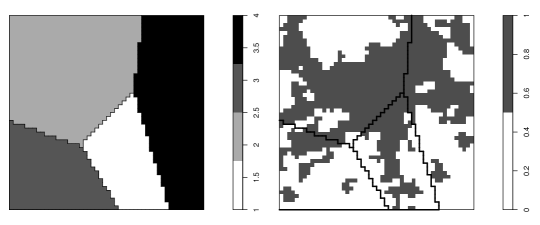
  Figure 3: Partition into 4 random sub-areas for Bologna dataset.

• compute Batty’s entropy for the phenomenon of interest, which may be "urban pixels" or "non-urban pixels"; one value for Batty’s entropy may be computed for each category of the variable, by specifying the argument category.
  

  R> bo.batty1=batty(boData, bo.part$data.assign, category=1,
  + win=bo.win, G.coords=bo.part$G.coords)
  R> bo.batty1$batty.ent
  

  [1] 7.788642
  

  R> bo.batty0=batty(boData, bo.part$data.assign, category=0,
  + win=bo.win, G.coords=bo.part$G.coords)
  R> bo.batty0$batty.ent
  

  [1] 7.795131

3.2.2 Point data

In this Section, the differences in the functions are highlighted between areal and point data, and between binary and multicategorical data. The workflow for computing Batty’s entropy for point pattern data with categorical marks, taking rainforest tree data as an example, is

• find the points’ coordinates, by exploiting coords.ppp from spatstat
  

  R>tree.cc=coords.ppp(treeData)
  

• partition the observation window into $G$ sub-areas
  

  R> tree.part=areapart(treeData$win, G=6, data.coords=tree.cc)
  

  where $G=6$ means six random centroids are generated over the window. The sub-areas borders are built following the Dirichlet tessellation (see ?dirichlet, a spatstat function), i.e. points are assigned to the area with the closest centroid. The area partition can be plotted with
  

  R> plot_areapart(bo.part$data.assign, bo.win, is.pointdata=T, add.data=T,
  + data.bin=T, category="rinosy", data=treeData,
  + G.coords=tree.part$G.coords, main="")

  where the option is.pointdata is set to TRUE. If the option add.data for displaying points is set to TRUE, for multicategorical data one can choose whether to plot all points or to select a category of interest. In the former case, data.bin=F (Figure 4, left panel), while in the latter case data.bin=T (Figure 4, right panel) for data dichotomization according to the specified category

  

  Figure 4: Partition into 6 random sub-areas for rainforest tree dataset. Left panel: all trees are plotted; right panel: only the specie Rinorea sylvatica is plotted.

• compute Batty’s entropy for a category of interest, with the option is.pointdata=T
  

  R> tree.batty.rinosy=batty(marks(treeData), tree.part$data.assign,
  + is.pointdata=T, category="rinosy", win=treeData$win,
  + G.coords=tree.part$G.coords)
  R> tree.batty.rinosy$batty.ent
  

  [1] 11.32699
  

3.3 Karlström and Ceccato’s entropy

A challenging attempt to introduce additive properties and to include the idea of neighbourhood in Batty’s entropy index (3) is due to Karlström and Ceccato (2002), following the LISA theory (Anselin, 1995). The adjacency matrix for $G$ spatial units is $A=\{a_{gg^{\prime}}\}_{g,g^{\prime}=1,\dots,G}$, a square $G\times G$ matrix such that $a_{gg^{\prime}}=1$ when $g^{\prime}\in\mathcal{N}(g)$, the neighbourhood of area $g$. In this proposal, the elements on the diagonal of the adjacency matrix $A$ are non-zero, i.e., each area neighbours itself.

Karlström and Ceccato’s entropy index $H_{KC}(F)$ starts by weighting the probability of occurrence of $F$ in a given spatial unit $g$, $p_{g}$, with its neighbouring values:

$$\widetilde{p}_{g}=\sum_{g^{\prime}=1}^{G}a_{gg^{\prime}}p_{g^{\prime}}.$$ (4)

Then, an information function is defined, fixing $T_{g}=1$, as $I(\widetilde{p}_{g})=\log\left(1/\widetilde{p}_{g}\right)$. Karlström and Ceccato’s entropy index is

$$H_{KC}(F)=E\left[I\left(\widetilde{p}_{g}\right)\right]=\sum_{g=1}^{G}p_{g}\log\left(\frac{1}{\widetilde{p}_{g}}\right).$$ (5)

The maximum of $H_{KC}(F)$ does not depend on the choice of the neighbourhood and is $\log(G)$. As the neighbourhood reduces, i.e., as $A$ tends to the identity matrix, $H_{KC}(F)$ tends to Batty’s spatial entropy (3), with equality in the case of $T_{g}=1$ for all $g$. The sum of local measures $L_{g}=p_{g}I(\widetilde{p}_{g})$ forms the global index (5), preserving the LISA property of additivity.

3.4 Karlström and Ceccato’s entropy with SpatEntropy

This is a modified version of Batty’s entropy, so one may refer to Section 3.2 for the necessary preamble. The key function is

karlstrom(data, data.assign, category, G.coords, neigh.dist)

where batty’s inputs is.pointdata and win are missing since they are needed for the computation of the areas $T_{g}$, which are discarded in this entropy measure. The only new input with regard to Batty’s entropy is neigh.dist; this is a scalar fixed by the user, expressing the extent of the neighbourhood in all directions. The value must be chosen keeping the area size into account.

3.4.1 Areal data

After all the steps needed for Batty’s entropy outlined in Section 3.2, for Bologna data, we write

R> bo.karlstr=karlstrom(boData, bo.part$data.assign, category=1,
+ bo.part$G.coords, neigh.dist=15)

$karlstrom.table
area.id abs.freq rel.freq p.tilde
[1,] 1 173 0.14076485 0.30634662
[2,] 2 580 0.47192840 0.30634662
[3,] 3 115 0.09357201 0.09357201
[4,] 4 361 0.29373474 0.29373474

$karlstrom.ent
[1] 1.306362

Setting neigh.dist=15 means that, when estimating $\widetilde{p}_{g}$ of (4) for a sub-area $g$, the proportions in all sub-areas whose centroid is at most 15 spatial units apart enter the computation. The output is analogous to the output of batty.

3.4.2 Point data

For point data with multicategorical marks, starting from the steps of Section 3.2, we write

R> tree.karlstr=karlstrom(marks(treeData), tree.part$data.assign,
+ category="rinosy", tree.part$G.coords, neigh.dist=100)

$karlstrom.table
area.id abs.freq rel.freq p.tilde
[1,] 1 30 0.0209937 0.1074178
[2,] 2 277 0.1938418 0.1074178
[3,] 3 258 0.1805458 0.1805458
[4,] 4 201 0.1406578 0.1406578
[5,] 5 341 0.2386284 0.2386284
[6,] 6 322 0.2253324 0.2253324

$karlstrom.ent
[1] 1.741951

where again neigh.dist is chosen by the user considering the total area size.

4 Entropy for spatially associated categorical variables

A second way to build a spatial entropy measure relies on defining a new categorical variable $Z$, where each realization identifies ordered couples $(x_{i},x_{j})$ of occurrences of $X$ over space. Order preservation within couples regards considering the relative spatial location of the observations. If order is preserved the couple $(x_{i},x_{j})$ implies that the observation carrying the $j$-th category occurs at the right or below the observation carrying the $i$-th category. Under this criterion, such couple is different from $(x_{j},x_{i})$. For $I$ categories of $X$, the new variable $Z$ has $R=I^{2}$ categories. The attention moves from the computation of (1), namely $H(X)$, to an index of the same form, Shannon’s entropy of $Z$, $H(Z)$.

The entropy measures based on $Z$ are useful when the variable of interest has two or more categories and when the goal is to understand how an outcome at one location affects neighbouring outcomes. Intuitively, when the variable is strongly spatially associated, neighbouring outcomes are closely related, which decreases the surprise (and thus, the entropy) in observing data. Such measures are based on selecting couples occurring at one specific distance; in the standard case, contiguous couples are considered, but extensions to farther distances are allowed. O’Neill and Leibovici’s entropies (O’Neill et al., 1988; Leibovici, 2009) quantify the residual amount of entropy associated to the variable of interest, once the influence of the spatial configuration has been taken into account at a specific distance. The chosen distance defines a neighbourhood, which is fixed prior to the analysis, and excludes information at farther distances. When the interest lies in what happens at contiguous locations, i.e., by considering areal units sharing a border, O’Neill’s entropy should be computed, or one of its contagion versions. When point data are available, or when distances other than contiguity are under study, Leibovici’s entropy should be used, which is a generalization of O’Neill’s entropy.

4.1 O’Neill’s entropy and contagion indices

O’Neill et al. (1988) propose one of the early spatial entropy indices for lattice data. It is based on computing a Shannon’s entropy (1) for the subset of the variable $Z$ made of contiguous couples, i.e., spatial realizations sharing a border. Such couples are identified by non-zero elements in the special adjacency matrix named contiguity matrix $C$. The subset of couples of contiguous realizations is $Z|C$, and its Shannon’s entropy is

$$H(Z|C)=\sum_{r=1}^{I^{2}}p(z_{r}|C)\log\left(\frac{1}{p(z_{r}|C)}\right).$$ (6)

Entropy (6) ranges from 0 to $\log(I^{2})$.

Other measures based on the construction of $Z|C$ start from the concept of contagion, the conceptual opposite of entropy. The Relative Contagion index $RC$ (Li and Reynolds, 1993) is proposed as

$$RC(Z|C)=1-H_{norm}(Z|C)=1-\frac{1}{\log(I^{2})}\sum_{r=1}^{I^{2}}p(z_{r}|C)\log\left(\frac{1}{p(z_{r}|C)}\right).$$ (7)

The second term is the normalized entropy of $Z|C$, via the multiplication of (6) by $1/\log(I^{2})$. Its complement to 1 is computed in order to measure relative contagion: the higher the spatial contagion between categories of $Z|C$, the lower the spatial entropy.

If one wants to account for the number of categories of $X$ when computing the contagion index, non-normalized measures should be computed in order to distinguish among contexts with different numbers of categories. For this reason, Parresol and Edwards (2014) suggest an unnormalized version of (7):

$$P(Z|C)=-H(Z|C)=\sum_{r=1}^{I^{2}}p(z_{r}|C)\log(p(z_{r}|C))$$ (8)

thus ranging from $-\log(I^{2})$ to $0$.

4.2 O’Neill’s entropy and contagion indices with SpatEntropy

The key function for O’Neill’s entropy is

leibovici(data, adj.mat, missing.cat = NULL, ordered = TRUE)

since, as explained in Section 4.3, O’Neill’s entropy is actually a special case of Leibovici’s entropy. As usual, data is a data matrix or vector, which can be numeric, factor, character. The input adj.mat is the contiguity matrix for O’Neill’s entropy and the contagion indices, i.e., a matrix identifying areal units sharing a border. The option missing.cat accounts for categories of the variable of interest that are absent in the dataset, while ordered is set as TRUE according to the authors’ choice to consider ordered couples of realizations.

4.2.1 Areal data and contiguity matrix

In order to compute O’Neill’s entropy and the contagion indices for Bologna lattice data, the starting point is the object bo.cc created in Section 3.2. Then, the workflow is

• compute the matrix of all Euclidean distances between pixel centroids
  

  R> bo.dmat=euclid_dist(bo.cc)
  

  Note that this SpatEntropy function may require some time for large datasets, but is only computed once and can then be used for any adjacency matrix and any entropy index. An alternative option is possible, which is faster though a little more complicated to program
  

  R> bo.ccP=ppp(bo.cc[,1], bo.cc[,2], bo.win)
  R> bo.dmat=pairdist(bo.ccP)
  R> bo.dmat[lower.tri(bo.dmat,diag=TRUE)] <- NA
  

  This option exploits spatstat functions: it turns the set of coordinates into a ppp object and uses the function pairdist to compute the distance between all pairs of centroids. Then, it turns the resulting symmetric matrix into a more efficient upper-triangular matrix

• build the contiguity matrix
  

  R> bo.adjmat=adj_mat(bo.dmat, dd0=0, dd1=1)
  

  where dd0 is the minimum distance and is always set to 0 for O’Neill’s entropy, while dd1 is equal to the pixel width in order to select only couples of pixels sharing a border (i.e., contiguous). The SpatEntropy function adj_mat builds an upper-triangular adjacency matrix, which means that couples of pixels are counted moving downward and rightward along the observation window. This ensures computational efficiency and avoids double counting of couples

• compute O’Neill’s entropy
  

  R> bo.oneill=leibovici(boData, bo.adjmat, ordered=T)
  

  This function makes use of the SpatEntropy function couple_count when ordered=T, (or the analogous pair_count when ordered=F) for building all possible adjacent couples in the dataset and computing the relative frequencies, which enter the computation of O’Neill’s entropy as estimates of the probabilities. The function leibovici returns a summary of the data structure, and the value of O’Neill’s entropy
  

  $freq.table
  couple abs.frequency proportion
  1 00 2159 0.44061224
  2 01 298 0.06081633
  3 10 315 0.06428571
  4 11 2128 0.43428571
  

  $entropy
  [1] 1.070045
  

The Relative Contagion index and Parresol and Edwards’ contagion can be computed in a similar way with the functions

contagion(oneill = NULL, n.cat = NULL, data = NULL, adj.mat = NULL,
missing.cat = NULL, ordered = TRUE)
parresol(oneill = NULL, n.cat = NULL, data = NULL, adj.mat = NULL,
missing.cat = NULL, ordered = TRUE)

The starting point for these indices may alternatively be oneill, the special output of leibovici as above, or the single raw inputs the same way as for leibovici. The only new input is n.cat which is the number of categories of the variable under study.

4.2.2 Point data and other computational options

The function is very flexible and allows to tune some options for computing entropy in an extended way. It can be used for point data; in such case, data is the mark vector. It allows for adjacency matrices different than the contiguity matrix, and for unordered couples (i.e., pairs). Some of these options are explored in Section 4.3. The possibility to work with pairs instead of couples is discussed in Section 5; for interpretation, remember that, if pairs are chosen instead of couples, the entropy value is smaller since the number of possible categories for $Z$ is smaller.

4.3 Leibovici’s entropy

Leibovici (2009) and Leibovici et al. (2014) propose a richer measure of entropy by extending $H(Z|C)$ in two ways. Firstly, $Z$ can now represent not only couples, but also triples and further degrees $m$ of co-occurrences. The authors develop the case of ordered co-occurrences, so that the number of categories of $Z$ is $R_{m}=I^{m}$. Secondly, space is now allowed to be continuous, so that areal as well as point data might be considered and associations may not coincide with contiguity: the concept of distance between occurrences replaces the concept of contiguity between lattice cells. A distance $d$ is fixed, then co-occurrences are defined for each $m$ and $d$ as $m$-th degree simultaneous realizations of $X$ at any distance $d^{*}\leq d$, i.e., distances are considered according to a cumulative perspective; this way an adjacency hypercube $A_{d}$ is built and the subset of interest is $Z|d$. Then, Leibovici’s spatial entropy is

$$H(Z|d)=\sum_{r=1}^{I^{m}}p(z_{r}|d)\log\left(\frac{1}{p(z_{r}|d)}\right).$$ (9)

In the case of lattice data, O’Neill’s entropy (6) is obtained as a special case when $m=2$ and $d$ equals the cell’s width.

4.4 Leibovici’s entropy with SpatEntropy

Leibovici’s entropy is currently implemented for couples ($m=2$) with the function leibovici. The key difference with regard to the examples of Section 4.2 is the possibility to choose the adjacency distance and to work with point data, not only with areal data.

4.4.1 Areal data

Leibovici’s entropy for Bologna data can be computed in a similar way to what illustrated in Section 4.2 for a generic distance

R> bo.adjmat5=adj_mat(bo.dmat, dd0=0, dd1=5)
R> bo.leib=leibovici(boData, bo.adjmat5, ordered=T)

where the value for the distance range of interest dd1 is set by the user. The output is analogous to the case in Section 4.2.

4.4.2 Point data

Leibovici’s entropy works the same way as for areal data for point data: a maximum distance range is chosen for the adjacency matrix, then couples are built by looking for points that lie within the distance range. The workflow, with the rainforest tree data example, is

• compute the matrix of all Euclidean distances between points (exploiting a spatstat function)
  

  R> tree.dmat=pairdist(treeData)
  R> tree.dmat[lower.tri(tree.dmat,diag=TRUE)] <- NA
  

• build the adjacency matrix for a chosen distance
  

  R> tree.adjmat=adj_mat(tree.dmat, dd0=0, dd1=20)
  

  where tree.adjmat is an upper-triangular adjacency matrix identifying all couples of trees at distance dd1 or less apart; dd1 is set by the user

• compute Leibovici’s entropy
  

  R> tree.leib=leibovici(marks(treeData), tree.adjmat, ordered=T)
  R> tree.leib$entropy
  

  [1] 0.7516415
  

Several Leibovici’s entropy values for different choices of dd1 may be compared; an example for the tree data is shown in Figure 5.

Figure 5: Leibovici’s entropy for tree data with $d=(5,10,20,50,100)$.

5 A decomposable spatial entropy measure

This is the most recent approach for spatial entropy measures. It should be employed when the interest lies in understanding the role of the spatial configuration in determining the entropy of a variable, not only at one isolated specific distance but also at a global level or at different distance ranges simultaneously. In addition, it should be used when the influence of space needs to be quantified as a percentage of the entropy. It is a more sophisticated approach from a statistical perspective, and allows more flexibility and interpretability than the previous measures.

The starting point is a different way of computing the variable $Z$ of Section 4; it is extendable to a general degree $m$ of co-occurrences (see Section 4.3), but it is currently implemented for pairs of realizations in SpatEntropy.

5.1 Altieri’s entropy

Altieri et al. (2018a) follow the approach based on $Z$ discarding order within co-occurrences, meaning that the relative spatial location of the two realizations is irrelevant; therefore, pairs are considered instead of couples. Discarding the order ensures a one-to-one correspondence between Shannon’s entropy of $X$ and $Z$. Moreover, ordering occurrences is not sensible in spatial statistics, where spatial configurations are not generally assumed to have a direction. Besides, when order is discarded, the number of categories of $Z$ is smaller. The gap between the two options grows as $I$ increases, and induces a different computational burden for large datasets.

A second discrete variable $W$ is introduced, that represents space by classifying the distances at which the two occurrences of a pair take place. Classes $w_{k}$ must be defined, with $k=1,\dots,K$, covering all possible distances within the observation window. Each distance class $w_{k}$ implies the choice of a corresponding adjacency matrix $A_{k}$, which identifies pairs where the two realizations of $X$ lie at a distance belonging to the range $w_{k}$.

Thanks to the introduction of $W$, the entropy of $Z$

$$H(Z)=\sum_{r=1}^{R}p(z_{r})\log\left(\frac{1}{p(z_{r})}\right)=MI(Z,W)+H(Z)_{W}$$ (10)

may be decomposed following the basis of Information Theory (Cover and Thomas, 2006). In (10), the two terms acquire a spatial meaning: $MI(Z,W)$ is spatial mutual information, quantifying the part of entropy of $Z$ due to the spatial configuration $W$; $H(Z)_{W}$ is spatial global residual entropy, quantifying the remaining information brought by $Z$ after space has been taken into account. The more $Z$ depends on $W$, i.e. the more the realizations of $X$ are spatially associated, the higher the spatial mutual information. Conversely, when the spatial association among the realizations of $X$ is weak, the entropy of $Z$ is mainly due to spatial global residual entropy. The entropy $H(Z)$ is a stable reference value, while its two components $MI(Z,W)$ and $H(Z)_{W}$ vary in order to evaluate the role of space for datasets with different spatial configurations. This is only the case when order is discarded. For the sake of interpretation and diffusion of the results, $MI_{prop}(Z,W)=MI(Z,W)/H(Z)$ may be used, which ranges in $[0,1]$ and is able to quantify the proportional contribution of space in the entropy of $Z$.

The overall value of $MI(Z,W)$, however, is often negatively influenced by what happens at large distance ranges, where usually scarce correlation is present. Hence, spatial mutual information for the whole dataset may be low even when a clustered pattern occurs. The variable $W$ helps in overcoming this drawback, since the two terms forming $H(Z)$ can be further decomposed. Indeed, $K$ subsets of realizations of $Z$ are available, denoted by $Z|w_{k}$. Spatial mutual information

$$MI(Z,W)=\sum_{k=1}^{K}p(w_{k})PI(Z|w_{k})$$ (11)

is a weighted sum of partial terms, where

$$PI(Z|w_{k})=\sum_{r=1}^{R}p(z_{r}|w_{k})\log{\left(\frac{p(z_{r}|w_{k})}{p(z_{r})}\right)}.$$ (12)

Each partial term $PI(Z|w_{k})$ quantifies the contribution to the departure from independence of each conditional distribution $p_{Z|w_{k}}$, i.e. the contribution of the $k$-th distance range to the global mutual information between $Z$ and $W$. Analogously, the following additive decomposition holds:

$$H(Z)_{W}=\sum_{k=1}^{K}p(w_{k})H(Z|w_{k}),$$ (13)

where the partial residual entropy terms measure the partial contributions to the entropy of $Z$ due to sources other than the spatial configuration:

$$H(Z|w_{k})=\sum_{r=1}^{R}p(z_{r}|w_{k})\log{\left(\frac{1}{p(z_{r}|w_{k})}\right)}.$$ (14)

5.2 Altieri’s entropy with SpatEntropy

The function for computing Altieri’s spatial entropy in SpatEntropy is

spat_entropy(data, adj.list, shannZ, missing.cat = NULL)

which relies on two other functions:

adj_list(dist.mat, dist.breaks)

and

shannonZ(data, missing.cat = NULL)

The function adj_list builds a list of adjacency matrices for a fixed partiton into distance classes. The function shannonZ starts from data, a data matrix or vector, and computes $H(Z)$ for unordered couples of realizations, exploiting the auxiliary SpatEntropy function pair_count. The outputs of the two functions enter spat_entropy as arguments adj.list and shannZ respectively. The output of spat_entropy is a list of estimates of all quantities of Section 5: mut.global, global spatial mutual information, res.global, global residual entropy, shannZ, Shannon’s entropy of $Z$, mut.local, partial information terms, res.local partial residual entropies, pwk, spatial weights for each distance range, pzr.marg, the relative frequencies of $Z$, pzr.cond, a $K$ dimensional list with the relative frequencies of $Z$ for each distance range, Q, the total number of pairs and Qk, the number of pairs for each distance range.

In the following, we help the user through practical implementation as well as interpretation of the results.

5.2.1 Areal data

The workflow for computing Altieri’s entropy for binary lattice data, using Bologna data, is

• compute Shannon’s entropy of $Z$
  

  R> bo.shZ=shannonZ(boData)
  

  The function returns the pair frequencies table and the benchmark value for Shannon’s entropy. Since the total number of possible pairs in the dataset is huge, this function may require a few minutes

• build the list of adjacency matrices by choosing the distance breaks according to the case study and the observation window’s size
  

  R> bo.maxdist=sqrt(diff(bo.win$xrange)^2+diff(bo.win$yrange)^2)
  R> bo.distbreaks=c(0,2,4,10,bo.maxdist)
  R> bo.adjlist=adj_list(bo.dmat, bo.distbreaks)
  

• compute Altieri’s entropy (which may take a few minutes on a standard laptop)
  

  R> bo.altieri=spat_entropy(boData, bo.adjlist, bo.shZ)
  

  An extract of the output is
  

  $mut.global
  [1] 0.005891553
  

  $res.global
  [1] 1.033506
  

  $shannZ
  [1] 1.039398
  

  $mut.local
  [1] 0.2365274495 0.1088072872 0.0319127643 0.0006132307
  

  $pwk
  [1] 0.004642497 0.013301961 0.087665786 0.894389756
  

Bologna’s dataset can be used for assessing urban heterogeneity; in this context, a compact city represents the desirable situation, where the $X$ outcomes are highly positively correlated. In such case, spatial mutual information should be high, because urban areas generally have urban neighbours, while non-urban areas have non-urban neighbours; space plays a relevant role in determining the entropy of $Z$. In this example, the entropy shannZ is $H(Z)=1.039$ and its two components are mut.global $MI(Z,W)=0.006$ and res.global $H(Z)_{W}=1.033$. The low value of $MI(Z,W)$ is due to the low value of its components mut.local $PI(Z|w_{k})$ at large ranges, which receive high weights pwk and influence the sum heavily: see the last partial values mut.local and the last weights pwk. Each partial information term measures the degree of association (compactness) in the city pattern at each distance range. The focus is on short distance ranges, where the difference between a compact city and a dispersed one is more evident: see the first mut.local values. By exploring these terms, an indication of the degree of dispersion can be provided.

Many plots can be produced for delivering the results. One example is shown in Figure 6: at each distance class, the sum $PI(Z|w_{k})+H(Z|w_{k})$ is set to 1, so that the contribution of space may be appreciated in proportional terms and is comparable. It is immediate to see that space explains one fifth of the data entropy at short distances, with a gradual decrease moving to large distance classes.

R> local.sum=bo.altieri$res.local+bo.altieri$mut.local
R> barplot(height=rbind(bo.altieri$mut.local/local.sum,
+ bo.altieri$res.local/local.sum), beside=F,
+ col=c("darkgray", "white"), names.arg=c("w1","w2","w3","w4"))

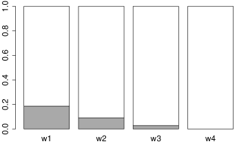
Figure 6: Altieri’s entropy for Bologna data: partial information (grey areas) and partial residual entropies (white areas) in proportional terms for each distance range.

5.2.2 Point data

The workflow for rainforest tree data is very similar, with the attention of using the vector of point marks as data and of tuning the distance breaks.

R> tree.shZ=shannonZ(marks(treeData), missing.cat=NULL)
R> tree.maxdist=sqrt(diff(treeData$win$xrange)^2+diff(treeData$win$yrange)^2)
R> tree.distbreaks=c(0,2,4,10,tree.maxdist)
R> tree.adjlist=adj_list(tree.dmat, tree.distbreaks)
R> tree.altieri=spat_entropy(marks(treeData), tree.adjlist, tree.shZ)

Useful guidelines for the interpretation of the results for rainforest tree data may be found in Altieri et al. (2018a).

6 Summary and discussion

In this paper, we introduce the new package SpatEntropy. Its version 0.1.0 contains 19 user-level functions which allow to implement spatial entropy measures. Central Sections 3, 4 and 5 separately introduce each of the main approaches to face spatial heterogeneity, and offer guidelines for choosing the most appropriate framework to measure spatial entropy, also according to the type of data.

When the hetoregeneity of the spatial distribution of a population needs to be evaluated according to a territory partitioned into sub-areas, Batty’s entropy of Section 3 should be used, or its development due to Karlström and Ceccato which includes a neighbourhood system. This approach has some disadvantages: a categorical variable $X$ with $I>2$ outcomes cannot be used for (3) and (5), since only one category enters the measure. In other words, computations have to be conducted for each specific category of $X$, thus $I$ different entropies are computed, but no way is proposed to synthesize them into a single spatial entropy measure for $X$. Moreover, these separate conclusions are heavily affected by the choice of the area partition.

For computing the entropy of a spatially correlated categorical variable, if data are areal and the focus is on the heterogeneity of contiguous realizations, then O’Neill’s entropy or the closely related contagion indices of Section 4 should be employed. Starting from a specific distance wider that contiguity and/or point data, O’Neill’s extension to Leibovici’s entropy of Section 4.3 can be used. The limit of these measures is that they only provide partial results. Indeed, O’Neill’s entropy only uses information about adjacent couples, and ignores the rest. Leibovici’s entropy works on the same principle, extending to a general distance $d$. Thus, if $d$ is small, a great part of the spatial information is not considered; conversely, if $d$ is large, the result is aggregate and excludes any possibility to explore the contribution of space in detail.

Lastly, if one wants to take a complete approach, which considers not only a single distance but all possible distance ranges to evaluate the overall influence of the spatial configuration in computing the data entropy, and which allows a flexible decomposition, then the recent Altieri’s approach of Section 5 is the most appropriate choice. The additive terms (12) and (14), together with their sums (11) and (13), constitute the set of spatial entropy measures. The approach is able to: maintain the information about the categories of $X$; consider different distance ranges simultaneously, by including an additional study variable representing space to enjoy the properties of bivariate entropy measures; quantify the overall role of space; be additive and decomposable. Therefore, spatial mutual information has in this case theoretical support to be considered the most reliable method for measuring data heterogeneity; it is also easily interpretable.

The package SpatEntropy works for areal and point data presenting a number of categories $I\geq 2$. It includes all necessary functions for extracting the spatial entropy of the data from scratch: the practical parts of Sections 3, 4 and 5 give step-by-step details.

User feedback is a fundamental part of the package development process. We welcome feedback and suggestions from all users.

References

- Altieri et al. (2014) Altieri, L., D. Cocchi, G. Pezzi, E. Scott, and M. Ventrucci (2014). Urban sprawl scatterplots for urban morphological zones data. Ecological Indicators 36, 315–323.
- Altieri et al. (2018a) Altieri, L., D. Cocchi, and G. Roli (2018a). A new approach to spatial entropy measures. Environmental and Ecological Statistics 25, 95–110.
- Altieri et al. (2018b) Altieri, L., D. Cocchi, and G. Roli (2018b). SpatEntropy: Spatial Entropy Measures. R package version 0.1.0.
- Anselin (1995) Anselin, L. (1995). Local indicators of spatial association - LISA. Geographical Analysis 27(2), 94–115.
- Baddeley et al. (2015) Baddeley, A., E. Rubak, and R. Turner (2015). Spatial Point Patterns: Methodology and Applications with R. London: Chapman and Hall/CRC Press.
- Batty (1974) Batty, M. (1974). Spatial entropy. Geographical Analysis 6, 1–31.
- Batty (1976) Batty, M. (1976). Entropy in spatial aggregation. Geographical Analysis 8, 1–21.
- Batty (2010) Batty, M. (2010). Space, scale, and scaling in entropy maximizing. Geographical Analysis 42, 395–421.
- Cover and Thomas (2006) Cover, T. M. and J. A. Thomas (2006). Elements of Information Theory. Second Edition. Hoboken, New Jersey: John Wiley & Sons, Inc.
- Cressie (1993) Cressie, N. (1993). Statistics for Spatial Data. Revised Edition. Hoboken, New Jersey: John Wiley & Sons, Inc.
- EEA (2011) EEA (2011). Analysing and managing urban growth. Technical report, Environmental European Agency. Also available as http://www.eea.europa.eu/articles/analysing-and-managing-urban-growth.
- Frosini (2004) Frosini, B. V. (2004). Descriptive Measures of Ecological Diversity. Paris, France. http://www.eolss.net: In Environmetrics. Edited by J. Jureckova, A. H. El-Shaarawi in Encyclopedia of Life Support Systems (EOLSS), revised edn. 2006. Developed under the Auspices of the UNESCO, Eolss Publishers.
- Karlström and Ceccato (2002) Karlström, A. and V. Ceccato (2002). A new information theoretical measure of global and local spatial association. The Review of Regional Research (Jahrbuch für Regionalwissenschaft) 22, 13–40.
- Leibovici (2009) Leibovici, D. G. (2009). Defining Spatial Entropy from Multivariate Distributions of Co-occurrences. Berlin, Springer: In K. S. Hornsby et al. (eds.): COSIT 2009, Lecture Notes in Computer Science 5756, pp 392-404.
- Leibovici et al. (2014) Leibovici, D. G., C. Claramunt, D. LeGuyader, and D. Brosset (2014). Local and global spatio-temporal entropy indices based on distance ratios and co-occurrences distributions. International Journal of Geographical Information Science 28(5), 1061–1084.
- Li and Reynolds (1993) Li, H. and J. F. Reynolds (1993). A new contagion index to quantify spatial patterns of landscapes. Landscape Ecology 8(3), 155–162.
- O’Neill et al. (1988) O’Neill, R. V., J. R. Krummel, R. H. Gardner, G. Sugihara, B. Jackson, D. L. DeAngelis, B. T. Milne, M. G. Turner, B. Zygmunt, S. W. Christensen, V. H. Dale, and R. L. Graham (1988). Indices of landscape pattern. Landscape Ecology 1(3), 153–162.
- Paninski (2003) Paninski, L. (2003). Estimation of entropy and mutual information. Neural Computation 15, 1191–1254.
- Parresol and Edwards (2014) Parresol, B. R. and L. A. Edwards (2014). An entropy-based contagion index and its sampling properties for landscape analysis. Entropy 16(4), 1842–1859.
- R Core Team (2017) R Core Team (2017). R: A Language and Environment for Statistical Computing. Vienna, Austria: R Foundation for Statistical Computing.
- Shannon (1948) Shannon, C. (1948). A mathematical theory of communication. Bell System Technical Journal 27(3), 379–423 and 27(4):623–656.
- Zhang (2012) Zhang, Z. (2012). Entropy estimation in turing’s perspective. Neural Computation 24, 1368–1389.